Iterative Feedback Tuning of Model-Free Intelligent PID Controllers

Abstract

In the last decades, model-free control (MFC) has become an alternative for complex processes whose models are not available or are difficult to obtain. Among the model-free control techniques, intelligent PID (iPID) algorithms, which are based on the ultralocal model parameterized with the constant α and including a classical PID, are used in many applications. This paper presents a new method for tuning iPID controllers based on the iterative feedback tuning (IFT) technique. This model-free tuning technique iteratively optimizes the parameters of a fixed structure controller using data coming from the closed-loop system operation. First, the discrete transfer functions of the iPID are deduced, considering the first and second order derivatives of the output variable from the ultralocal model. Using the discrete transfer functions, the iPID controllers become the fixed structure type, and the IFT parameter tuning method can be applied. Thus, in addition to the classical gains of the PID algorithm, the value of the parameter α is also obtained, which is usually determined by trial-and-error. The performances of the IFT-tuned iPID controllers were experimentally tested and validated in real-time using Quanser AERO 2 laboratory equipment with a one degree of freedom (1-DOF) configuration.

1. Introduction

Due to current advanced hardware and software technologies, data acquisition, storage, computing, and communication allow for the processing of increased amounts of data online. In this way, a new method referred to as data-driven control (DDC) has been developed, by which the controllers are directly designed using input–output data collected from the control system without process modeling. Through the development of information technology, the industrial processes have become more complex, making their modeling difficult. An alternative to the model-based control method is DDC, which has rapidly developed in recent decades. Overviews on the model-based control and data-driven control techniques are presented in [1,2], while the DDC theory is covered in books such as [3,4,5]. At the same time, the data-driven tuning techniques were developed to optimize the controller parameters, distinguishing two classes based on the controller structure. The first class is intended for controllers with a fixed structure. Among these, the iterative feedback tuning (IFT) algorithm [6] iteratively optimizes the controller parameters by estimating the gradient of a cost function in relation to the input and output signals; the virtual reference feedback tuning (VRFT) method [7] is a direct data-driven method to optimize the controller parameters, which does not require iterations. The second class includes tuning methods that do not require knowledge of the regulator structure, such as iterative learning control [8] or model-free adaptive control [4].

One DDC method is the model-free control (MFC) algorithm, which was developed by Fliess and Join [9] and has been successfully applied in many fields. It is based on the use of the ultralocal model, which is valid for a short time interval and is on the embedded of a PID controller in the control law, which is called an intelligent PID (iPID). The tuning parameters of the iPID controller are the usual tuning gains of the PID controller, to which the non-physical constant parameter α from the ultralocal model is added. Considering the ultralocal model and closing the tuning loop with the iPID controller, a description of the control system is obtained through a linear differential equation of the control error, which only depends on the tuning gains of the PID, if a good estimate of the term including the unknown parts of the ultralocal model is available [8]. Hence, the conclusion from [8] is made, where tuning the iPID controller is easy to perform by enforcing the condition that the differential equation must have stable roots, thus canceling the steady-state error. Furthermore, in accordance with a condition from [9,10], the user will choose the parameter α. Although it seems easy to tune an iPID controller, the use of only the linear differential equation does not directly lead to achieving the tuning gains.

For tuning the iPID controllers, several methods have been reported in the literature. Starting from the tuning proposed in [8] based on the cancellation of the control error in the steady-state, in [11,12], domains were determined in the tuning gains space, for which the stability of the roots of the error differential equation is ensured, thus obtaining a zero steady-state error. The VRFT one-shot data-driven tuning algorithm can be used to tune the iPID controllers. Thus, in [13], the method is shown regarding how the VRFT algorithm can be used to tune the iP, iPI, and iPID model-free controllers, where the three tuned controllers are validated on modular servo system laboratory equipment. Another hybrid method is generated by mixing the model-free control with the sliding mode control (SMC) [14], resulting in a simple design method that ensures the stability of the tracking error dynamics specific to MFC. If the MFC in [14] is of the iPI type, the method in [15] presents the MFC-SMC with an iPD controller intended for the attitude and position control of a quadrotor.

The design methods above lead to the acquisition of the tuning gains of the iPID controllers without the possibility of finding a suitable value for $\alpha$, which remains a constant design parameter to be chosen by the user according to [9,10]. However, other methods have been proposed to determine the parameter, such as in [16], where $\alpha$ is found using an algorithm based on the ultralocal model. Another approach considers $\alpha$ as a time-varying parameter for which the values are instantly estimated [17,18].

The data-driven IFT method for tuning controllers with a fixed structure is a gradient descent-based iterative algorithm presented in [6], are both theoretical aspects and applications regarding the tuning of controllers for mechanical and chemical systems. The tuning objective is to obtain the step response of the closed-loop system with a minimal settling time and small overshoot. The advantages of applying the IFT method for tuning PID controllers in relation to the classic methods are presented in [19]. To ensure the con-vergence for the initial parameters of the controller, [20] presents a solution based on a domain of attraction (DoA) approach. With respect to the regulatory control system, several solutions have proposed the use of the IFT algorithm. By using a special experiment, the authors of [21] describe the gradient estimate method based on a spectral analysis; in [22], the authors suggest the correlation-based IFT algorithm to reduce the influence of noise from the collected data. Solutions that do not require a special experiment to estimate the gradient related to the feedforward controller have also been proposed, such as those presented in [23,24]. A constrained IFT method was introduced in [25] for the robust cascade path-tracking control of a networked robot. For a model-free adaptive iterative learning controller, the IFT algorithm was used in [26] for controller parameters tuning. A first attempt of using the IFT algorithm for tuning a model-free iP controller intended for the speed control of an engine was presented in [27].

This paper proposes a new method for tuning the model-free iPID controllers based on the IFT data-driven algorithm. Being a data-driven approach, a process model is not required to tune the controller parameters; it only requires the sets of input–output data collected from the control system. Because the IFT algorithm is a method for tuning the parameters of a controller with a fixed structure, this study first determined a structure for the iPID controller using the connections between the iPID and PID discrete-time controllers. Only the first and second order derivatives related to the ultralocal model, which is the basis of the model-free control concept, were considered. Using the derivative approximation method based on the backward difference, the fixed structures of the iPID controllers were obtained, which were described by discrete transfer functions that were parameterized with a parameter vector. Based on these discrete transfer functions, behaviors that assimilated to those of conventional PID controllers were found, which allowed for the selection of intelligent controllers with behaviors like the PID ones and the removal of those with unusual behaviors in the control engineering process. Knowing the fixed structures of the iPID controllers, the IFT data-driven algorithm was applied, and the optimal tuning parameters of the controllers were obtained. The proposed tuning method based on IFT data-driven algorithms has the advantage of generating iPID tuning parameters related to the PID control law, but also the parameter $\alpha$, which was usually chosen by the user. The new iPID controller tuning method based on the IFT algorithm is illustrated by real-time experiments that are aimed to validate the tuned controllers. The experiments were conducted with Quanser AERO 2 laboratory equipment in the one degree of freedom (1-DOF) configuration, with two DC motors for driving the propellers, for which the pitch angle was controlled.

This laboratory equipment, due to offering a wide range of system structures obtained through half-quad (pitch-locked, yaw-free), 1-DOF (yaw-locked, pitch-free), or 2-DOF con-figurations [28], was often used for testing and validating new control methods. For all configurations, the control with PID regulators is presented in [28]. New control algorithms for the 2-DOF configuration can also be found in the literature, such as adaptive neural control [29], approximation-based quantized state feedback tracking [30], observer-based sliding mode control [31], fuzzy neural networks [32], or adaptive attitude control with input and output quantization [33].

This paper proposes the following new contributions with respect to the state-of-the-art:

(i)

A new method of tuning model-free iPID controllers based on the IFT algorithm;

(ii)

The calculation of both the tuning gains of the iPID controller and the parameter $\alpha$;

(iii)

The determination of a fixed structure for iPID controllers based on the connections between the iPID and PID discrete-time controllers to make it possible to apply the IFT tuning algorithm;

(iv)

An analysis of the connections between the iPID and PID controllers; model-free control laws that correspond to some variants of the classical PID were determined, and those which are uncommon in the control engineering process were eliminated;

(v)

The tuning of the iPID controllers using the IFT algorithm was tested and validated experimentally on Quanser AERO 2 laboratory equipment.

The paper is organized as follows. Section 2 discusses the connections between the iPID and PID controllers, and based on them, the fixed structure of the iPID controller is presented. Section 3 first briefly introduces the IFT approach and then describes how to tune the iPID controller using the IFT algorithm. The experimental validation of the tuned iPID controllers is shown in Section 4, and Section 5 concludes the paper.

2. iPID Fixed Structure Based on Connections between the iPID and PID Discrete-Time Controllers

The IFT technique is a model-free technique used to iteratively optimize the parameters of a fixed-order controller using data coming from the closed-loop system operation. Applying the IFT technique for tuning an iPID controller first requires the determination of a fixed structure for this type of controller, which is parametrized by a vector $\rho \in {ℝ}^n$. For this reason, the discrete form of the iPID controllers has been related to the classical PID, which has a fixed structure.

The MFC method is designed around the concept of the ultralocal model [9], which is obtained from signals of the system and is available for a very short time frame. The equation that describes the ultralocal model, with notations from the operational calculus, is:

$$s^{\nu }Y(s)=F(s)+\alpha U(s),$$

(1)

where $Y$ is the output signal of the system, $U$ is the control signal, $\alpha$ is a parameter chosen by the practitioner, and $F$ is a function which contains all of the unmodelled components of the ultralocal model. The derivative order $\nu$ of $y$ is usually chosen as 1 or 2 [9]. The control law iPID is defined as:

$$U(s)=\frac{1}{\alpha }\left(s^{\nu }\tilde{Y}(s)-F(s)+\left(K_p+\frac{K_i}{s}+K_{d}s\right)E(s)\right),$$

(2)

where $\tilde{Y}$ is the reference signal, $E=\tilde{Y}-Y$ is the control error, and $K_p$, $K_i$, and $K_d$ are the tuning gains of a classical PID controller.

The discrete-time ultralocal model is obtained using the backward difference approximation, as suggested in [34], by replacing $s$ with $\left(1-z^{-1}\right)/T_s$, where $T_s$ is the sampling period, resulting in:

$${\left(\frac{1-z^{-1}}{T_s}\right)}^{\nu }{y}_k=F_k+\alpha u_k.$$

(3)

Using Equation (3), the estimation of the unmodelled components of the ultralocal model is defined as:

$${\widehat{F}}_k={\left(\frac{1-z^{-1}}{T_s}\right)}^{\nu }{y}_k-\alpha u_{k-1}.$$

(4)

In the following, the estimation error between the actual $F_k$ and its estimation ${\widehat{F}}_k$ is considered negligible.

Applying the backward difference approximation to Equation (2) and using the estimation from Equation (4), the discrete-time iPID control law is obtained:

$$u_k=\frac{1}{\alpha (1-z^{-1})}\left({\left(\frac{1-z^{-1}}{T_s}\right)}^{\nu }{e}_k+\left(K_p+K_i\frac{T_s}{1-z^{-1}}+K_d\frac{1-z^{-1}}{T_s}\right)e_k\right).$$

(5)

From Equation (5), the discrete-time classical PID control law is easily deduced:

$$u_k=\left(K_p+K_i\frac{T_s}{1-z^{-1}}+K_d\frac{1-z^{-1}}{T_s}\right)e_k.$$

(6)

Next, the connections between the discrete-time iPID and PID controllers will be investigated, considering the two recommended values for the derivative order $\nu$.

First, for $\nu =1$, from Equation (5) after a simple calculation, the following form of the iPID₁ regulator results:

$$u_k=\frac{1}{\alpha }\left(\frac{1+K_d}{T_s}{e}_k+\frac{K_p}{T_s}\frac{T_s}{1-z^{-1}}{e}_k+\frac{K_i}{T_s}\frac{T_s^2}{{(1-z^{-1})}^2}{e}_k\right),$$

(7)

which highlights a classical PI-I² type controller. The subscript of iPID₁ indicates the derivative order $\nu =1$.

Using Equation (7), the following equations are obtained for the intelligent controllers iP₁, iPI₁, and iPD₁, by setting the appropriate tuning parameters. Thus, for $K_i=K_d=0$, the iP₁ control law is found:

$$u_k=\frac{1}{\alpha }\left(\frac{1}{T_s}{e}_k+\frac{K_p}{T_s}\frac{T_s}{1-z^{-1}}{e}_k\right),$$

(8)

which corresponds to a classical PI controller. If only $K_d=0$, the result is the iPI₁ control law:

$$u_k=\frac{1}{\alpha }\left(\frac{1}{T_s}{e}_k+\frac{K_p}{T_s}\frac{T_s}{1-z^{-1}}{e}_k+\frac{K_i}{T_s}\frac{T_s^2}{{(1-z^{-1})}^2}{e}_k\right),$$

(9)

which has the form of a PI-I² controller, as in the case of the iPID₁ controller, but with different tuning parameters. Setting $K_i=0$, the iPD₁ control law is obtained:

$$u_k=\frac{1}{\alpha }\left(\frac{1+K_d}{T_s}{e}_k+\frac{K_p}{T_s}\frac{T_s}{1-z^{-1}}{e}_k\right),$$

(10)

which is a classical PI controller, as in the case of the iP₁ controller, but with different tuning parameters. When analyzing the comparisons between the iPID₁ and classical PID controllers for $\nu =1$, it is discovered that the intelligent controllers behave like PI or PI-I². For the iP₁ and iPD₁ controllers that behave like PI, by applying the Z transform to Equations (8) and (10), the discrete transfer function results:

$$G_{iP\&D}{}_{{}_1}(z^{-1})=\frac{q_0+q_1{z}^{-1}}{1-z^{-1}},$$

(11)

whose tuning parameters grouped in the vector $\rho ={[q_0 q_1]}^T$ are determined according to the type of the intelligent controller, as follows:

$${\mathrm{iP}}_1: q_0=\frac{1+T_s{K}_p}{\alpha T_s},q_1=-\frac{1}{\alpha T_s},$$

(12)

$${\mathrm{iPD}}_1: q_0=\frac{1+K_d+\alpha T_s{K}_p}{\alpha T_s},q_1=-\frac{1+K_d}{\alpha T_s}.$$

(13)

Applying the Z transform to Equations (7) and (9), the discrete transfer function of the iPI₁ and iPID₁ controllers that behave like PI-I² is obtained:

$$G_{iPI\&D_1}(z^{-1})=\frac{q_0+q_1{z}^{-1}+q_2{z}^{-2}}{1-2z^{-1}+z^{-2}},$$

(14)

with the following tuning parameters grouped in the vector $\rho ={[q_0 q_1 q_2]}^T$:

$${\mathrm{iPI}}_1: q_0=\frac{K_p{T}_s+1}{\alpha T_s}, q_1=-\frac{K_p{T}_s+K_i{T}_s^2+2}{\alpha T_s}, q_2=\frac{1}{\alpha T_s},$$

(15)

$${\mathrm{iPID}}_1: q_0=\frac{K_p{T}_s+K_i{T}_s^2+K_d+1}{\alpha T_s}, q_1=-\frac{K_p{T}_s+2K_d+2}{\alpha T_s}, q_2=\frac{1+K_d}{\alpha T_s}$$

(16)

In conclusion, for $\nu =1$, the intelligent controllers iP₁ and iPD₁ behave as a PI controller, having a fixed structure given by the discrete transfer function from Equation (11), parametrized by a vector $\rho \in {ℝ}^2$; the intelligent controllers iPI₁ and iPID₁ behave like a PI-I² controller with a fixed-order structure, given by the discrete transfer function from the Equation (14), parametrized by a vector $\rho \in {ℝ}^3$.

For $\nu =2$, using Equation (5), the iPID₂ control law is obtained:

$$u_k=\frac{1}{\alpha }\left(\frac{K_d}{T_s}{e}_k+\frac{K_p}{T_s}\frac{T_s}{1-z^{-1}}{e}_k+\frac{1}{T_s}\frac{1-z^{-1}}{T_s}{e}_k+\frac{K_i}{T_s}\frac{T_s^2}{{(1-z^{-1})}^2}{e}_k\right),$$

(17)

which highlights a classical PID-I² controller. The subscript of iPID₂ indicates the derivative order $\nu =2$.

Similar to the case of $\nu =1$, by setting the tuning parameters in Equation (17), the control laws iP₂, iPI₂, and iPD₂ for $\nu =2$ are obtained. Therefore, for $K_i=K_d=0$, the iP₂ control law is achieved:

$$u_k=\frac{1}{\alpha }\left(\frac{K_p}{T_s}\frac{T_s}{1-z^{-1}}{e}_k+\frac{1}{T_s}\frac{1-z^{-1}}{T_s}{e}_k\right),$$

(18)

with a classical ID controller behavior, which is uncommon in the control engineering. Considering only $K_d=0$, the control law iPI₂ is obtained:

$$u_k=\frac{1}{\alpha }\left(\frac{K_p}{T_s}\frac{T_s}{1-z^{-1}}{e}_k+\frac{1}{T_s}\frac{1-z^{-1}}{T_s}{e}_k+\frac{K_i}{T_s}\frac{T_s^2}{{(1-z^{-1})}^2}{e}_k\right),$$

(19)

which is equivalent to a classical ID-I² controller, also unused in the control engineering. Setting $K_i=0$, the iPD₂ control law results in:

$$u_k=\frac{1}{\alpha }\left(\frac{K_d}{T_s}{e}_k+\frac{K_p}{T_s}\frac{T_s}{1-z^{-1}}{e}_k+\frac{1}{T_s}\frac{1-z^{-1}}{T_s}{e}_k\right),$$

(20)

having a classical PID behavior.

Considering only the iPD₂ and iPID₂ controllers and applying the Z transform to Equations (17) and (20), which are related to the two controllers, the iPD₂ discrete transfer function is obtained:

$$G_{iP{D}_2}(z^{-1})=\frac{q_0+q_1{z}^{-1}+q_2{z}^{-2}}{1-z^{-1}},$$

(21)

and, respectively, for iPID₂:

$$G_{iPI{D}_2}\left(z^{-1}\right)=\frac{q_0+q_1{z}^{-1}+q_2{z}^{-2}+q_3{z}^{-3}}{1-2z^{-1}+z^{-2}}.$$

(22)

The parameter vectors for the two controllers and the expressions of the tuning parameters are:

$${\mathrm{iPD}}_2: \rho ={[q_0 q_1 q_2]}^T; \mathrm{with}:q_0=\frac{K_p{T}_s^2+K_d{T}_s+1}{\alpha T_s^2},q_1=-\frac{K_d{T}_s+2}{\alpha T_s^2},q_2=\frac{1}{\alpha T_s^2},$$

(23)

$$\begin{gathered} {\mathrm{iPID}}_2: \rho ={[q_0 q_1 q_2 q_3]}^T; \mathrm{with}: q_0=\frac{1+K_p{T}_s^2+K_d{T}_s}{\alpha T_s^2}, \\ {q}_1=-\frac{3+K_p{T}_s^2-K_i{T}_s^3+2K_d{T}_s}{\alpha T_s^2}, q_2=\frac{2+K_d{T}_s}{\alpha T_s^2},q_3=-\frac{1}{\alpha T_s^2}. \end{gathered}$$

(24)

Analyzing for the case of $\nu =2$ in the comparisons between the iPID₂ and the classic PID controllers, it turned out that the iP₂ and iPI₂ controllers behave similarly to equivalent classical controllers, which is unusual in the control engineering. The iPD₂ and iPID₂ controllers, PID and PID-I² type behaviors, and fixed structures expressed by the transfer functions from Equations (21) and (22) were found, which were parameterized by the vectors $\rho$ given by Equations (23) and (24).

The connections analyzed between the iPID and PID showed that both for $\nu =1$ and for $\nu =2$, the intelligent controllers have either an integrator or an integrator supplemented by a double integrator. It also resulted that a derivative behavior of the iPID controllers was only obtained for $\nu =2$.

The parameters vector $\rho$ will be determined using the model-free IFT approach. Because the tuning parameters $K_p$, $K_i$, $K_d$, and $\alpha$ are obtained based on the $\rho$ vector, only the iP₁ and iPI₁ controllers were chosen for $\nu =1$; this is because from Equations (12) and (15), unique solutions for the tuning gains and $\alpha$ are obtained. At the same time, for the case of $\nu =1$, the neglected controllers iPD₁ and iPID₁ have the same type of behavior as the iP₁ and iPI₁ controllers; however, from Equations (13) and (16), unique solutions for the tuning parameters and $\alpha$ are not obtained.

In the following, we will consider $\nu =1$ for the controllers iP₁ and iPI₁, having the fixed structure described by the transfer functions $G_{i{P}_1}$ and $G_{iP{I}_1}$, given by Equations (11) and (14); we will also consider $\nu =2$ for the controllers iPD₂ and iPID₂ with the fixed structure described by the transfer functions $G_{iP{D}_2}$ and $G_{iPI{D}_2}$, provided by Equations (21) and (22).

3. Model-Free IFT for iPID Controllers

3.1. Iterative Feedback Tuning Approach

It is considered a linear time-invariant discrete-time process with unknown dynamics controlled by a linear discrete-time controller with a fixed-order structure described by a discrete transfer function $G_c\left(\rho \right)$ and parameterized with the $\rho$ vector. For this controller, the minimization of some norm of the error between the achieved and the desired response over the controller parameter vector $\rho$:

$$e_k(\rho )=y_k(\rho )-{\tilde{y}}_k,$$

(25)

is imposed as a design objective. For IFT, the following quadratic criterion is used:

$$J(\rho )=\frac{1}{2N}\{{\displaystyle \sum _{k=1}^N{(L_y{e}_k(\rho ))}^2}+\lambda {\displaystyle \sum _{k=1}^N(L_u{u}_k}(\rho ){)}^2\},$$

(26)

where $y_k(\rho )$ represents the output of the system after using the set of parameters $\rho$ for the controller, ${\tilde{y}}_k$ represents the reference signal of the control system, and $u_k(\rho )$ is the control signal for the used set of parameters $\rho$. $L_y$ and $L_u$ are filters that weighted the output and control signals, $\lambda$ is a penalty factor, and N is the number of samples. The cost function from Equation (26) will be minimized by an optimal parameter vector:

$${\rho }^{\ast }=\arg \underset{\rho }{\min }J(\rho ).$$

(27)

A necessary condition to obtain the minimum is the cancellation of the derivative of $J\left(\rho \right)$ with respect to the vector parameters $\rho$. Considering for simplicity $L_y=L_u=1$, the derivative of $J\left(\rho \right)$ becomes:

$$\frac{\partial J}{\partial \rho }(\rho )=\frac{1}{N}[{\displaystyle \sum _{k=1}^N{e}_k(\rho )\frac{\partial e_k}{\partial \rho }(\rho )}+\frac{\lambda }{N}{\displaystyle \sum _{k=1}^N{u}_k(\rho )\frac{\partial u_k}{\partial \rho }(\rho )}].$$

(28)

If the gradient $\frac{\partial J}{\partial \rho }(\rho )$ could be computed using Equation (28), the solution of the equation $\frac{\partial J}{\partial \rho }(\rho )=0$ can be obtained in an iterative way, as follows:

$${\rho }_{i+1}={\rho }_i-{\gamma }_i{R}_i^{-1}\frac{\partial J}{\partial \rho }({\rho }_i),$$

(29)

where ${\gamma }_i$ is a positive real scalar that determines the step size, whereas $R_i$ is a symmetric positive defined matrix used to update the direction. To obtain the negative gradient descent direction, the identity matrix is usually used. Furthermore, using the data collected from the control system, the matrix defined by:

$$R_i=\frac{1}{N}{\displaystyle \sum _{k=1}^N(\left[\frac{\partial y_k}{\partial \rho }({\rho }_i)\right]{\left[\frac{\partial y_k}{\partial \rho }({\rho }_i)\right]}^T+\lambda \left[\frac{\partial u_k}{\partial \rho }({\rho }_i)\right]{\left[\frac{\partial u_k}{\partial \rho }({\rho }_i)\right]}^T}.$$

(30)

can be employed [6].

Because the exact gradient is not known, it is replaced in Equation (29) by an unbiased estimate $\frac{\partial \widehat{J}}{\partial \rho }({\rho }_i)$. To determine the unbiased estimate $\frac{\partial \widehat{J}}{\partial \rho }({\rho }_i)$, the following quantities are needed:

(i)

The signals $e_k({\rho }_i)$ and $u_k({\rho }_i)$;

(ii)

The estimation of the gradients $\frac{\partial e_k}{\partial \rho }\left({\rho }_i\right)$ and $\frac{\partial u_k}{\partial \rho }\left({\rho }_i\right)$;

(iii)

Unbiased estimates of the products $e_k\frac{\partial e_k}{\partial \rho }\left({\rho }_i\right)$ and $u_k\frac{\partial u_k}{\partial \rho }\left({\rho }_i\right)$.

These quantities are obtained through closed-loop experiments with the controller, having the transfer function $G_c$ parameterized with the $\rho$ vector.

From Equation (25), it follows:

$$\frac{\partial e_k}{\partial \rho }({\rho }_i)=\frac{\partial y_k}{\partial \rho }({\rho }_i),$$

(31)

and thus, the estimations from (ii) refer to the output and input signals.

Denoting the closed loop transfer function with $G_0$ and the sensitivity function with $S$, the following expressions of the derivatives of the output and input signals were obtained in [6]:

$$\begin{array}{l}\frac{\partial y_k}{\partial \rho }({\rho }_i)=\frac{1}{G_c({\rho }_i)}\frac{\partial G_c}{\partial \rho }({\rho }_i)G_0({\rho }_i)\left(r-y_k({\rho }_i)\right)\\ \frac{\partial u_k}{\partial \rho }({\rho }_i)=\frac{1}{G_c({\rho }_i)}\frac{\partial G_c}{\partial \rho }({\rho }_i)S({\rho }_i)\left(r-y_k({\rho }_i)\right)\end{array}$$

(32)

At iteration $i$, with the fixed controller $G_c\left({\rho }_i\right)$ being known, its derivative can be calculated. With the controller $G_c\left({\rho }_i\right)$ in the closed loop, based on two experiments of length $N$ denoted by (a) and (b), the derivatives from Equation (32) are estimated. For the first experiment (a), the reference of the control loop is $\tilde{y}$, resulting in:

$$\begin{array}{l}{\tilde{y}}_i^{(a)}=\tilde{y}\\ y_k^{(a)}({\rho }_i)=G_0({\rho }_i)\tilde{y}\\ u_k^{(a)}({\rho }_i)=S({\rho }_i)G_c({\rho }_i)\tilde{y}\end{array}$$

(33)

The second experiment (b) is a special one. The reference is $\tilde{y}-y_k^{(a)}({\rho }_i)$, and the output/input signals are:

$$\begin{array}{l}{\tilde{y}}_i^{(b)}=\tilde{y}-y_k^{(a)}({\rho }_i)\\ y_k^{(b)}({\rho }_i)=G_0({\rho }_i)\left(\tilde{y}-y_k^{(a)}({\rho }_i)\right)\\ u_k^{(b)}({\rho }_i)=S({\rho }_i)G_c({\rho }_i)\left(\tilde{y}-y_k^{(a)}({\rho }_i)\right)\end{array}$$

(34)

The superscript (a) and (b) used in Equations (33) and (34) indicate that the signals were obtained during experiment (a) and (b).

Based on the signals obtained in the two experiments, the estimation of the output/input gradients is determined as it is suggested in [6]:

$$\begin{array}{l}est\left[\frac{\partial y_k}{\partial \rho }({\rho }_i)\right]=\frac{1}{G_c({\rho }_i)}\frac{\partial G_c}{\partial \rho }({\rho }_i)y_k^{(b)}({\rho }_i),\\ est\left[\frac{\partial u_k}{\partial \rho }({\rho }_i)\right]=\frac{1}{G_c({\rho }_i)}\frac{\partial G_c}{\partial \rho }({\rho }_i)u_k^{\left(b\right)}({\rho }_i).\end{array}$$

(35)

With the estimations from the Equation (35) obtained based on the two experiments, the unbiased estimate $\frac{\partial \widehat{J}}{\partial \rho }({\rho }_i)$ of the cost function can be computed with:

$$\frac{\partial \widehat{J}}{\partial \rho }({\rho }_i)=\frac{1}{N}\{[{\displaystyle \sum _{k=1}^N{e}_k({\rho }_i)est\left[\frac{\partial y_k}{\partial \rho }({\rho }_i)\right]}+\frac{\lambda }{N}{\displaystyle \sum _{k=1}^N{u}_k({\rho }_i)est\left[\frac{\partial u_k}{\partial \rho }({\rho }_i)\right]}\}.$$

(36)

The same estimates available after the two experiments are used to estimate the matrix $R_i$, defined by (30), which becomes:

$${\widehat{R}}_i=\frac{1}{N}{\displaystyle \sum _{k=1}^N(est\left[\frac{\partial y_k}{\partial \rho }({\rho }_i)\right]est{\left[\frac{\partial y_k}{\partial \rho }({\rho }_i)\right]}^T+\lambda est\left[\frac{\partial u_k}{\partial \rho }({\rho }_i)\right]est{\left[\frac{\partial u_k}{\partial \rho }({\rho }_i)\right]}^T}.$$

(37)

Using the estimates given by Equations (36) and (37), the iterative calculation of the tuning parameters with Equation (29) turns to:

$${\rho }_{i+1}={\rho }_i-{\gamma }_i{\widehat{R}}_i^{-1}\widehat{\frac{\partial J}{\partial \rho }}({\rho }_i).$$

(38)

The following algorithm gives the steps of the IFT approach:

• In the first iteration, the tuning parameters of the controller are chosen in such a way as to obtain a stable response in the closed loop.
• At each iteration $i$, two experiments of length $N$ are performed:

  (a)

  The reference $\tilde{y}$ is applied to the control system, and the input/output signals are collected ${\left\{u_k^{\left(a\right)}\left({\rho }_i\right),y_k^{\left(a\right)}\left({\rho }_i\right)\right\}}_{k=\overline{1,N}}$;

  (b)

  The reference $\tilde{y}-y_k^{(a)}({\rho }_i)$ is applied to the control system, and the input/output signals are collected ${\left\{u_k^{\left(b\right)}\left({\rho }_i\right),y_k^{\left(b\right)}\left({\rho }_i\right)\right\}}_{k=\overline{1,N}}$;

• The estimates for the gradients of $u_k\left({\rho }_i\right)$ and $y_k\left({\rho }_i\right)$ are calculated by Equation (35);
• Using the estimates from Step 3, the gradient estimates for the cost function $\frac{\partial \widehat{J}}{\partial \rho }({\rho }_i)$ and for the matrix ${\widehat{R}}_i$ are determined with Equations (36) and (37), respectively;
• Based on the estimates from Equations (36) and (37), the new vector of parameters ${\rho }_{i+1}$ is calculated with Equation (38);
• Repeat Step 2–5 until the optimal vector of parameters ${\rho }^{*}$ is obtained.

The IFT algorithm presented in this section can be applied for the calculation of gradient approximations in the case of nonlinear systems from the collected experimental data [35]. The solution proposed by Hjalmarsson in [6,35] is to generate the true gradient using the linear time-varying system obtained by linearizing the nonlinear system around the system trajectory under normal operating conditions. In this context, the same IFT procedure as the one used for linear systems can be applied.

3.2. IFT of iPID Controllers

For tuning the iPID controllers with the IFT approach, the discrete transfer functions obtained in the previous Section for $\nu =1$ ($G_{i{P}_1}$ and $G_{iP{I}_1}$) and $\nu =2$ ($G_{iP{D}_2}$ and $G_{iPI{D}_2}$) will be considered:

$$\begin{array}{l}{G}_{i{P}_1}(z^{-1})=\frac{q_0+q_1{z}^{-1}}{1-z^{-1}},\\ G_{iP{I}_1}(z^{-1})=\frac{q_0+q_1{z}^{-1}+q_2{z}^{-2}}{1-2z^{-1}+z^{-2}},\\ G_{iP{D}_2}(z^{-1})=\frac{q_0+q_1{z}^{-1}+q_2{z}^{-2}}{1-z^{-1}},\\ G_{iPI{D}_2}\left(z^{-1}\right)=\frac{q_0+q_1{z}^{-1}+q_2{z}^{-2}+q_3{z}^{-3}}{1-2z^{-1}+z^{-2}}.\end{array}$$

(39)

Based on these transfer functions, for the estimations of the output and input quantities with Equation (35), the derivatives of the transfer functions, weighted with their inverses, are firstly calculated for each type of iPID controller, as follows:

• iP₁ controller

$$\begin{array}{l}\frac{1}{G_{i{P}_1}}\frac{\partial G_{i{P}_1}}{\partial q_0}=\frac{1}{q_0+q_1{z}^{-1}},\\ \frac{1}{G_{i{P}_1}}\frac{\partial G_{i{P}_1}}{\partial q_1}=\frac{z^{-1}}{q_0+q_1{z}^{-1}}.\end{array}$$

(40)

• iPI₁ controller

$$\begin{array}{l}\frac{1}{G_{iP{I}_1}}\frac{\partial G_{iP{I}_1}}{\partial q_0}=\frac{1}{q_0+q_1{z}^{-1}+q_2{z}^{-2}},\\ \frac{1}{G_{iP{I}_1}}\frac{\partial G_{iP{I}_1}}{\partial q_1}=\frac{z^{-1}}{q_0+q_1{z}^{-1}+q_2{z}^{-2}},\\ \frac{1}{G_{iP{I}_1}}\frac{\partial G_{iP{I}_1}}{\partial q_2}=\frac{z^{-2}}{q_0+q_1{z}^{-1}+q_2{z}^{-2}}.\end{array}$$

(41)

• iPD2 controller

$$\begin{array}{l}\frac{1}{G_{iP{D}_2}}\frac{\partial G_{iP{D}_2}}{\partial q_0}=\frac{1}{q_0+q_1{z}^{-1}+q_2{z}^{-2}},\\ \frac{1}{G_{iP{D}_2}}\frac{\partial G_{iP{D}_2}}{\partial q_1}=\frac{z^{-1}}{q_0+q_1{z}^{-1}+q_2{z}^{-2}},\\ \frac{1}{G_{iP{D}_2}}\frac{\partial G_{iP{D}_2}}{\partial q_2}=\frac{z^{-2}}{q_0+q_1{z}^{-1}+q_2{z}^{-2}}.\end{array}$$

(42)

• iPID2 controller

$$\begin{array}{l}\frac{1}{G_{iPI{D}_2}}\frac{\partial G_{iPI{D}_2}}{\partial q_0}=\frac{1}{q_0+q_1{z}^{-1}+q_2{z}^{-2}+q_3{z}^{-3}},\\ \frac{1}{G_{iPI{D}_2}}\frac{\partial G_{iPI{D}_2}}{\partial q_1}=\frac{z^{-1}}{q_0+q_1{z}^{-1}+q_2{z}^{-2}+q_3{z}^{-3}},\\ \frac{1}{G_{iPI{D}_2}}\frac{\partial G_{iPI{D}_2}}{\partial q_2}=\frac{z^{-2}}{q_0+q_1{z}^{-1}+q_2{z}^{-2}+q_3{z}^{-3}},\\ \frac{1}{G_{iPI{D}_2}}\frac{\partial G_{iPI{D}_2}}{\partial q_3}=\frac{z^{-3}}{q_0+q_1{z}^{-1}+q_2{z}^{-2}+q_3{z}^{-3}}.\end{array}$$

(43)

Applying the above algorithm, the optimal parameter vectors ${\rho }^{*}$ are obtained for each individual iPID controller, and based on them, the tuning parameters $K_p$, $K_i$, $K_d$, and α are calculated using Equations (15), (16), (23), and (24), with the results being summarized in

Table 1. Tuning parameters.

	${\mathit{K}}_{\mathit{p}}$	${\mathit{K}}_{\mathit{i}}$	${\mathit{K}}_{\mathit{d}}$	$\mathit{\alpha }$
iP1	$-\frac{q_0+q_1}{q_1{T}_s}$			$-\frac{1}{q_1{T}_s}$
iPI1	$\frac{q_0-q_2}{q_2{T}_s}$	$-\frac{q_0+q_1+q_2}{q_2{T}_s^2}$		$\frac{1}{T_s{q}_2}$
iPD2	$\frac{q_0+q_1+q_2}{q_2{T}_s^2}$		$-\frac{q_1+2q_2}{q_2{T}_s}$	$\frac{1}{q_2{T}_s^2}$
iPID2	$\frac{q_2-q_0+q_3}{q_3{T}_s^2}$	$-\frac{q_0+q_1+q_2}{q_3{T}_s^3}$	$-\frac{q_2+2q_3}{q_3{T}_s}$	$-\frac{1}{q_3{T}_s^2}$

.

4. Case Studies—Real-Time Control of Pitch Angle for Aero 2 Laboratory Equipment

To test and validate the iPID controllers tuning using the IFT algorithm, we considered a real-time application for controlling the pitch angle for the dual-motor aerospace system Aero 2, provided by Quanser. The system has two rotors that can be used for various aerospace applications, with the possibility to control the pitch and yaw angles as suggested in [28,29,30,31,32,33]. To control the pitch angle, the 1-DOF configuration was chosen for the Aero 2 platform, which locks the yaw and has the pitch as free. This configuration, represented in Figure 1, was used for real-time experiments, having both propellers horizontal and ensuring a variation of the pitch angle of 90° degrees, 45° degrees for each side.

Single-ended optical shaft encoders were used to measure the pitch of the Aero body and the angular speed of the DC motors [28]. The pitch encoder is 2880 counts per revolution in quadrature mode, and the angular speed encoder is a counter that returns the number of the encoder counts every second.

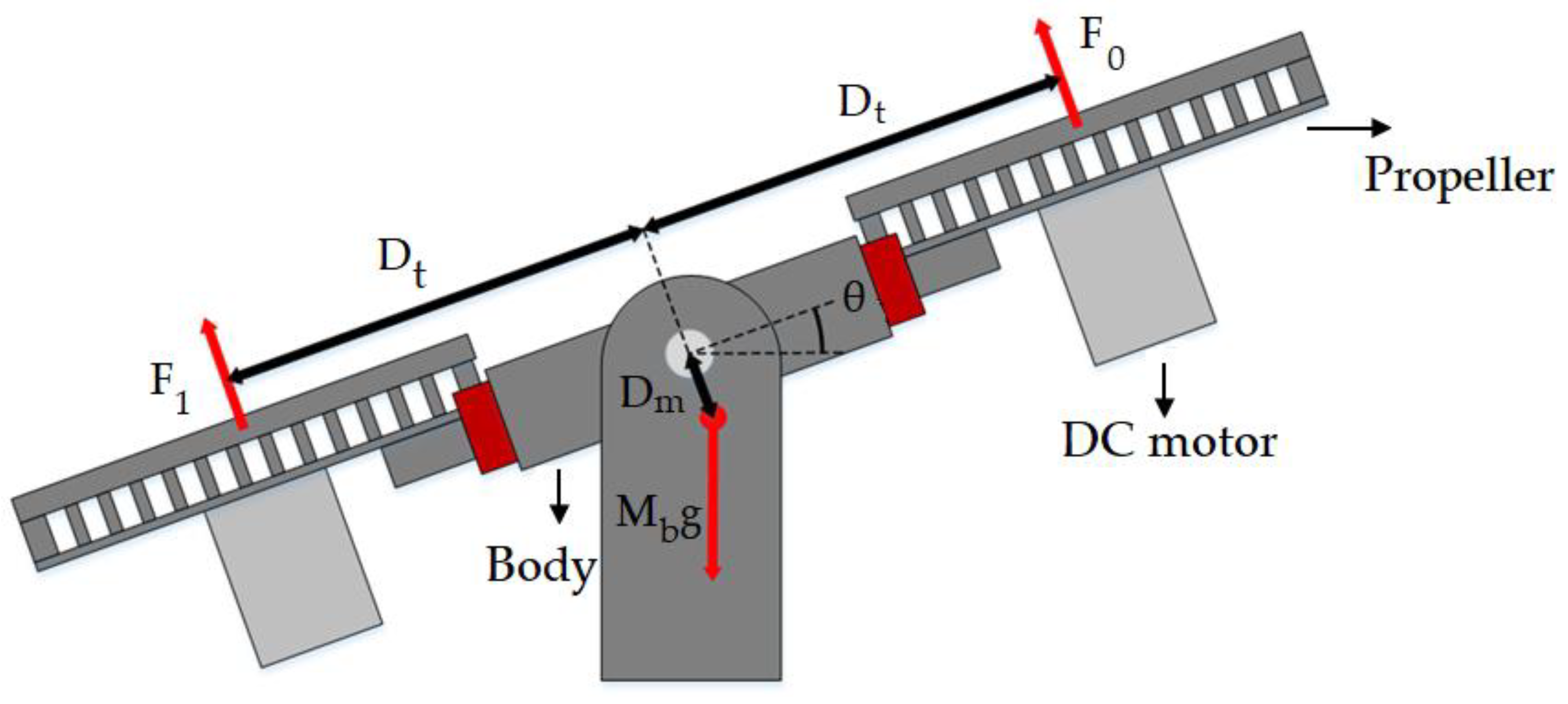
The scheme of the 1-DOF Aero 2 plant for the pitch angle control is shown in Figure 2, where $M_b$ is the aero body mass, $D_t$ is the thrust displacement, $D_m$ is the center of mass displacement, and $\theta$ is the pitch angle to the equilibrium position; $F_0$ and $F_1$ are the thrust forces generated by propellers that are driven by two DC motors, and g is the gravitational acceleration. To introduce nonlinearities, an asymmetry was created by using a single propeller operating in both positive and negative thrust and by shifting the center of mass towards thruster 1.

Each propeller was driven by a DC motor, its supply voltage $v_m$ being considered the input variable, and the output variable is the pitch angle $\theta$. The plant model was obtained based on the DC motor and propeller models.

The DC motor dynamics are described by [28]:

$$\begin{array}{l}{L}_m\frac{d{i}_m}{dt}=v_m-R_m{i}_m-e_b\\ J_m\frac{d{\omega }_m}{dt}={\tau }_m-{\tau }_d\\ e_b=k_e{\omega }_m\\ {\tau }_m=k_m{i}_m\end{array}$$

(44)

where $i_m$ is the motor current, $R_m$ and $L_m$ are the resistance and inductances of the rotor, $e_b$ is the back electromotive force (emf), $J_m$ is the rotor inertia, ${\omega }_m$ is the motor angular speed, ${\tau }_m$ is the motor torque, ${\tau }_d$ is the drag torque and $k_e$ and $k_m$ are the motor back EMF and torque constant. Neglecting the rotor inductance, an assumption valid for low-power motors, the following model of the DC motor results from Equation (44):

$$J_m\frac{d{\omega }_m}{dt}=-\frac{k_e{k}_m}{R_m}{\omega }_m+\frac{k_m}{R_m}{v}_m-{\tau }_d$$

(45)

The dynamic behavior of the propeller system can be modeled by taking into account [28] and [29,31]:

$$\begin{array}{l}\left(J_p+M_b{D}_m^2\right)\ddot{\theta }+D_p\dot{\theta }+K_{sp}\theta +M_{b}g{D}_m\cos \theta ={\tau }_p\\ {\tau }_p=K_{pp}{\omega }_m{D}_t\end{array}$$

(46)

where $J_p$ is the moment of inertia related to the pitch motion, $D_p$ is the viscous damping coefficient, $K_{sp}$ is the stiffness, $K_{pp}$ is the force thrust gain relative to the rotor speed, $D_t$ is the distance from the pivot point to the center of the rotor, and ${\tau }_p$ is the torque acting on the pitch axis, created by the thrust force $F=K_{pp}{\omega }_m$.

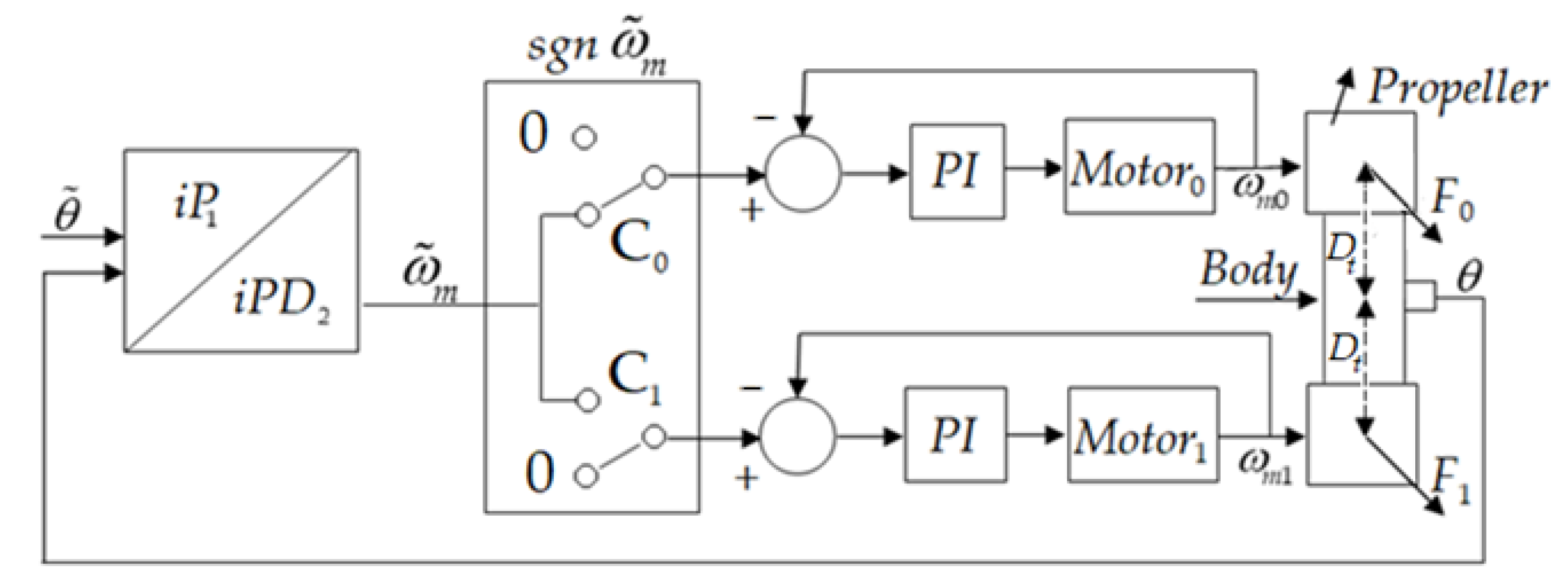
Considering the models of the two components of the plant, a cascade control structure was chosen, with a faster inner loop for controlling the motor angular speed ${\omega }_m$ and an outer loop for controlling the pitch angle $\theta$. In this way, the disturbance introduced by the drag torque ${\tau }_d$ will be rejected. The cascade control structure is a special one, whose scheme is represented in Figure 3.

The $C_0$ and $C_1$ switches, which depend on the sign of the angular velocity reference ${\tilde{\omega }}_m$, have been introduced to activate a single motor. Thus, for ${\tilde{\omega }}_m>0$, the related internal propeller loop that generates the thrust force $F_0$ will come into operation, and for ${\tilde{\omega }}_m<0$, it will be the propeller that generates the thrust force $F_1$. The presence of the two switches, through which a single inner loop is activated depending on the sign of ${\tilde{\omega }}_m$, introduces a nonlinearity in the control system. Another nonlinearity from Equation (46) is created by the asymmetric placement of the center of gravity, as seen in Figure 2.

For each inner loop, a PI controller described by [28]:

$$u=-k_p{\omega }_m+k_i\left({\tilde{\omega }}_m-{\omega }_m\right)$$

(47)

was designed, starting from the simplified model (45) of the DC motor and considering the overshoot $\sigma$ and peak time $t_p$ as desired performances, as in [28]. Applying the Laplace transform to the DC motor model (45), a first-order transfer function is obtained with gain $k=1/k_e$ and time constant $\tau =J_m{k}_m{k}_e/R_m$. Using the plant transfer function, in [28], the following tuning parameters of the PI controller were obtained based on a pole placement method:

$$\begin{array}{l}{k}_p=\left(2\zeta {\omega }_n\tau -1\right)/k\\ k_i={\omega }_n^2\tau /k\end{array}$$

(48)

where the damping ratio $\zeta$ and natural frequency ${\omega }_n$ are calculated based on the desired performances. Employing the DC motor parameters and the desired performances from [28], the following tuning parameters of the inner loop PI controller were obtained: $k_p=0.1553, k_i=2.3176$.

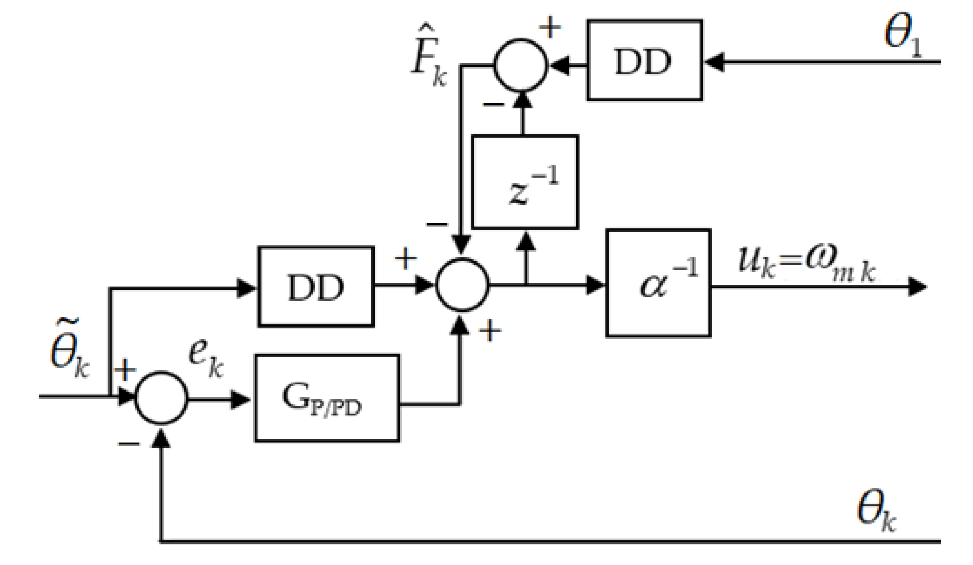
For the outer loop, two model-free controllers were tested to validate the proposed design method based on the data-driven IFT algorithm. The first one tested was an iP₁ controller with a PI-type behavior, as shown in Section 2, which ensures a zero steady-state error; the second one was an iPD₂ with a PID-type behavior, for which the influence of the derivative component was analyzed. The structures of the two model-free controllers are depicted in Figure 4.

In the model-free controller structure, the Discrete Derivative block DD computes the discrete-time derivative using the backward difference approximation; the $G_{P/PD}$ block implements the discrete transfer function of the P or PD controller, resulting in the iP₁ or iPD₂ controllers. The sample time $T_s=0.002 \mathrm{s}$ for both controllers was considered due to the small value of the time constants of the inner loop.

The outer loop plant is formed by the closed-loop transfer function of the inner loop, to which the propeller model from Equation (46) is added. Although the closed-loop model of the inner loop is known by designing with the pole placement method, the propeller model is considered as totally unknown. The design of the model-free controller was conducted only based on the data collected from the control system without using any outer loop plant model.

The Aero 2 system from Quanser was connected with a PC, where the control scheme from Figure 2 was implemented using MATLAB/Simulink 2021b software tools.

For tuning the two model-free controllers, the IFT algorithm from Section 3 was used, which is based on two closed-loop experiments and the collection of input and output data related to the real-time experiments. The proposed aero pitch controller tuning methodology is the following:

• In the first step of the IFT algorithm, the tuning parameters of the two controllers that lead to a stable response must be found. These parameters were determined as in [11] and [12] based on the characteristic polynomial of the error, for which it was required that the roots be stable, thus cancelling the error in the steady-state. For iP₁, it follows from [11] that the roots of the characteristic polynomial of the error are stable if $K_p\in \left(0,2/T_s\right)$. Applying the Jury test, the domain in the plane of gains parameters, where the roots of the characteristic polynomial are stable, was obtained in [12] for the iPD₂ controller, defined by:

  $$\begin{array}{l}{T}_s^2{K}_p>0\\ 4-2T_s{K}_d+T_s^2{K}_p>0\\ \left|1+T_s^2{K}_p-T_s{K}_d\right|<1\end{array}$$

  (49)

For the two model-free controllers, the initial tuning parameters were chosen using values from the stability domains of the roots. With the tuning parameters thus determined, an experiment is carried out, and if undesirable performances are obtained, proceed to Step 2 of the IFT algorithm.

2.

At each iteration $i$, two experiments of length $N=30/T_s$ are performed:

(a)

The reference $\tilde{\theta }=0.2 \mathrm{rad}$ is applied to the pitch control system, and the input/output signals are collected ${\left\{u_k^{\left(a\right)}\left({\rho }_i\right),{\theta }_k^{\left(a\right)}\left({\rho }_i\right)\right\}}_{k=\overline{1,N}}$;

(b)

The reference $\tilde{\theta }-{\theta }_k^{(a)}({\rho }_i)$ is applied to the control system, and the input/output signals are collected ${\left\{u_k^{\left(b\right)}\left({\rho }_i\right),{\theta }_k^{\left(b\right)}\left({\rho }_i\right)\right\}}_{k=\overline{1,N}}$.

3.

Based on the data ${\left\{u_k^{\left(b\right)}\left({\rho }_i\right),{\theta }_k^{\left(b\right)}\left({\rho }_i\right)\right\}}_{k=\overline{1,N}}$ collected in the special experiment (b), the estimates of the gradients for $u_k\left({\rho }_i\right)$ and ${\theta }_k\left({\rho }_i\right)$ and the estimates of the gradient of the cost function $\widehat{\frac{\partial J}{\partial \rho }}({\rho }_i)$ and for the matrix ${\widehat{R}}_i$, described by (37), are computed.

4.

Using the estimates from Step 3, the new vector of parameters ${\rho }_{i+1}$ is calculated; based on the vector, the tuning parameters are determined using Table 1.

5.

With the tuning parameters determined in Step 4, the performances of the pitch control system are tested in a real-time experiment.

6.

If the performances obtained with the tuning parameters from Step 5 are not satisfactory, restart the tuning procedure by repeating Step 2–5 until the desired performances are reached.

The penalty factor $\lambda$ from Equation (26) and the step size ${\gamma }_i$ from Equation (29) were determined through a trial-and-error procedure, while the matrix $R_i$ was considered the identity matrix $I_n$, one of possibilities mentioned by [6] and [36]. To test the performances of the control system for each iteration $i$ of the tuning procedure, the ITAE (integral time-weighted absolute error) criterion defined by:

$$ITA{E}_i={\displaystyle \sum _{k=1}^{N}k{T}_s\left|e_k\right|}$$

(50)

was used, where $k{T}_s$ is the discrete-time expressed in seconds. This criterion is helpful because the objective is to have a smooth response without oscillations around the reference value.

4.1. Control of Pitch Angle with iP₁ Controller

Based on the stability condition of the roots of the characteristic polynomial, the iP_1-0 controller with the tuning parameters from

Table 2. Tuning parameters for the iP₁ controllers and the ITAE criteria values.

Iteration	Initial Values		ITAE	Final Values
1	$\begin{array}{l}{K}_{p-0}=17.5\\ {\alpha }_0=28\end{array}$	$\begin{array}{l}{q}_{0-0}=18.4821\\ q_{1-0}=-17.8571\end{array}$	$\begin{array}{l}ITA{E}_0=\\ \mathrm{43,517}\end{array}$	$\begin{array}{l}{K}_{p-1}=17.352\\ {\alpha }_1=27.9959\end{array}$	$\begin{array}{l}{q}_{0-1}=18.4795\\ q_{1-1}=-17.8597\end{array}$
2	$\begin{array}{l}{K}_{p-1}=17.352\\ {\alpha }_1=27.9959\end{array}$	$\begin{array}{l}{q}_{0-1}=18.4795\\ q_{1-1}=-17.8597\end{array}$	$\begin{array}{l}ITA{E}_1=\\ \mathrm{43,428}\end{array}$	$\begin{array}{l}{K}_{p-2}=17.1917\\ {\alpha }_2=27.9971\end{array}$	$\begin{array}{l}{q}_{0-2}=18.4768\\ q_{1-2}=-17.8625\end{array}$
3	$\begin{array}{l}{K}_{p-2}=17.1917\\ {\alpha }_2=27.9971\end{array}$	$\begin{array}{l}{q}_{0-2}=18.4768\\ q_{1-2}=-17.8625\end{array}$	$\begin{array}{l}ITA{E}_2=\\ \mathrm{43,419}\end{array}$	$\begin{array}{l}{K}_{p-3}=17.0322\\ {\alpha }_3=27.9871\end{array}$	$\begin{array}{l}{q}_{0-3}=18.4739\\ q_{1-3}=-17.8654\end{array}$
4	$\begin{array}{l}{K}_{p-3}=17.0322\\ {\alpha }_3=27.9871\end{array}$	$\begin{array}{l}{q}_{0-3}=18.4739\\ q_{1-3}=-17.8654\end{array}$	$\begin{array}{l}ITA{E}_3=\\ \mathrm{43,205}\end{array}$	$\begin{array}{l}{K}_{p-4}=16.8649\\ {\alpha }_3=27.9825\end{array}$	$\begin{array}{l}{q}_{0-4}=18.4710\\ q_{1-4}=-17.8683\end{array}$
Final	$\begin{array}{l}{K}_{p-IFT}=16.8649\\ {\alpha }_{IFT}=27.9825\end{array}$	$\begin{array}{l}{q}_{0-IFT}=18.4710\\ q_{1-IFT}=-17.8683\end{array}$	$\begin{array}{l}ITA{E}_4=\\ \mathrm{43,175}\end{array}$

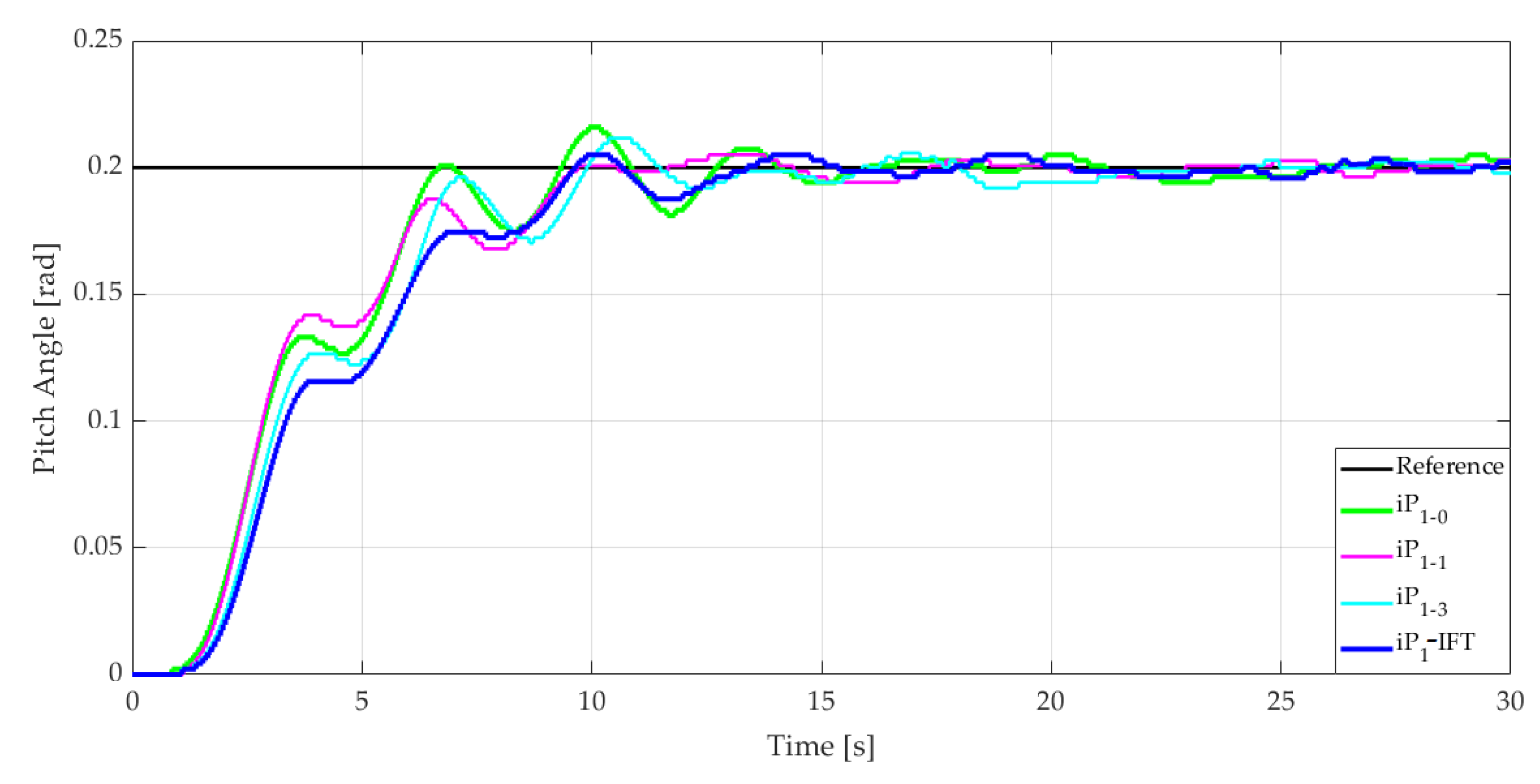
were chosen for the initial step. Using step size ${\gamma }_i=0.0003$, penalty factor ${\lambda }_i=0.001$, and matrix $R_i=I_2$, four iterations of the IFT algorithm have been created, resulting in the controllers iP_1-1,2,3 and finally the fourth controller, iP₁-IFT. The stopping point was determined based on the optimum performance criterion defined by Equation (50). The responses of the iP₁ controllers are shown in Figure 4, where the unsatisfactory performances of the iP_1-0 controller are visible. The IFT tuning procedure was applied in order to improve the performances. The initial response of the control system and other several intermediate responses results obtained with the iP_1-1,3 and iP₁-IFT controllers during the tuning procedure are shown in Figure 5.

In Figure 5, the system responses obtained with the iP₁ controllers are represented by considering the tuning parameters found using the tuning methodology. The optimal values have been obtained in the fourth step. The responses from the figure show that during the application of the IFT algorithm, the oscillations of the output signal become more damped and thus, the settling time decreases.

The parameters ${\rho }_i$ and the values of the tuning parameters of the iP₁ controllers, which were determined with the relationships from Table 1, are presented in Table 2 together with the values of the ITAE criteria for each iteration.

In Table 2, the values of the ITAE criterion decrease with the increase in the number of iterations, indicating the performances improvement.

The iP_1-0 and iP₁-IFT controllers are used in a comparative experiment, which in-volves modifications of the reference signal, with different steps, in both directions of the pitch axis. The result of the comparison is depicted in Figure 6, from which the good behavior of the iP₁-IFT controller in relation to iP_1-0 is shown.

The control signals for the iP₁-₀ and iP₁-IFT controllers during the comparison experiments are presented in Figure 7. Therein represented are the reference angular speed of the motors ${\tilde{\omega }}_m$ and, at the same time, the responses of the two inner loops generated by the C₀ and C₁ switches from Figure 3, depending on $\mathrm{sgn}{\tilde{\omega }}_m$. When ${\tilde{\omega }}_m>0$, the reference generated by the iP₁ controller of the outer loop will be applied through C₀ to the inner loop related to the motor₀, and the inner loop of the motor₁ will have the reference equal to zero through switch C₁. For ${\tilde{\omega }}_m<0$, the switches change their position and thus, the inner loop related to the motor₁ will receive the reference; for motor₀, the reference will be zero. The operation of the switches according to $\mathrm{sgn}{\tilde{\omega }}_m$ introduces a nonlinearity in the plant model related to the outer loop.

From Figure 7, an oscillating operation is observed for the DC motors, which actuate the propellers for the iP_1-0 controller, which can cause the wear of the Aero 2 system. These oscillations disappear in the case of the iP₁-IFT controller.

4.2. Control of Pitch Angle with the iPD₂ Controller

As shown in the conclusions from Section 2, the iPD₂ controller will introduce a derivative component that accelerates the control loop and leads to a faster response of the system, but at the same time amplifying the high-frequency signals. A similar procedure with the iP₁ case presented in Section 4.1 was created, starting with a stable response of the system with an iPD_2-0 controller that was now determined based on the Jury test. For the iPD₂ controller, five iterations of the IFT algorithm have been achieved with step size ${\gamma }_i=0.000025$, penalty factor ${\lambda }_i=0.1$, and matrix $R_i=I_3$. The responses obtained during the tuning phase with the initial controller iPD_2-0, with some intermediate controllers iPD_2-2,3 and the final controller iPD₂-IFT, are presented in Figure 8.

The system controlled with iPD_2-0 shows oscillations with high amplitude, which are reduced after five iterations of the IFT algorithm. This gives the system a high range, where it can reach the reference for the pitch angle. The iPD_2-5 from the final iteration, noted as iPD₂-IFT, was chosen due to the obtained performances, which have been evaluated according to the ITAE criterion from Equation (50). The damping of the oscillations during the tuning phase leads to the decrease in the settling time, which becomes smaller than the one obtained with the iP₁-IFT controller in Figure 5 due to the derivative component. In

Table 3. Tuning parameters for the iPD₂ controllers and the ITAE criteria values.

Iteration	Initial Values		ITAE	Final Values
1	$\begin{array}{l}{K}_{p-0}=20\\ K_{d-0}=20\\ {\alpha }_0=24\end{array}$	$\begin{array}{l}{q}_{0-1}=\mathrm{10,834}.17\\ q_{1-1}=-\mathrm{21,250}.00\\ q_{2-1}=\mathrm{10,416}.67\end{array}$	$\begin{array}{c}ITA{E}_0=\\ 1401\end{array}$	$\begin{array}{l}{K}_{p-1}=19.0842\\ K_{d-1}=20.0019\\ {\alpha }_1=24\end{array}$	$\begin{array}{l}{q}_{0-1}=\mathrm{10,834}.15\\ q_{1-1}=-\mathrm{21,250}.01\\ q_{2-1}=\mathrm{10,416}.65\end{array}$
2	$\begin{array}{l}{K}_{p-1}=19.0842\\ K_{d-1}=20.0019\\ {\alpha }_1=24\end{array}$	$\begin{array}{l}{q}_{0-1}=\mathrm{10,834}.15\\ q_{1-1}=-\mathrm{21,250}.01\\ q_{2-1}=\mathrm{10,416}.65\end{array}$	$\begin{array}{c}ITA{E}_1=\\ 1369\end{array}$	$\begin{array}{l}{K}_{p-2}=18.0803\\ K_{d-2}=20.0039\\ {\alpha }_2=24.0001\end{array}$	$\begin{array}{l}{q}_{0-2}=\mathrm{10,834}.14\\ q_{1-2}=-\mathrm{21,250}.03\\ q_{2-2}=\mathrm{10,416}.64\end{array}$
3	$\begin{array}{l}{K}_{p-2}=18.0803\\ K_{d-2}=20.0039\\ {\alpha }_2=24.0001\end{array}$	$\begin{array}{l}{q}_{0-2}=\mathrm{10,834}.14\\ q_{1-2}=-\mathrm{21,250}.03\\ q_{2-2}=\mathrm{10,416}.64\end{array}$	$\begin{array}{c}ITA{E}_2=\\ 1317\end{array}$	$\begin{array}{l}{K}_{p-3}=17.0496\\ K_{d-3}=20.0060\\ {\alpha }_3=24.0001\end{array}$	$\begin{array}{l}{q}_{0-3}=\mathrm{10,834}.13\\ q_{1-3}=-\mathrm{21,250}.04\\ q_{2-3}=\mathrm{10,416}.63\end{array}$
4	$\begin{array}{l}{K}_{p-3}=17.0496\\ K_{d-3}=20.0060\\ {\alpha }_3=24.0001\end{array}$	$\begin{array}{l}{q}_{0-3}=\mathrm{10,834}.13\\ q_{1-3}=-\mathrm{21,250}.04\\ q_{2-3}=\mathrm{10,416}.63\end{array}$	$\begin{array}{c}ITA{E}_3=\\ 1295\end{array}$	$\begin{array}{l}{K}_{p-4}=16.0102\\ K_{d-4}=20.0081\\ {\alpha }_4=24.0001\end{array}$	$\begin{array}{l}{q}_{0-4}=\mathrm{10,834}.11\\ q_{1-4}=-\mathrm{21,250}.06\\ q_{2-4}=\mathrm{10,416}.61\end{array}$
5	$\begin{array}{l}{K}_{p-4}=16.0102\\ K_{d-4}=20.0081\\ {\alpha }_4=24.0001\end{array}$	$\begin{array}{l}{q}_{0-4}=\mathrm{10,834}.11\\ q_{1-4}=-\mathrm{21,250}.06\\ q_{2-4}=\mathrm{10,416}.61\end{array}$	$\begin{array}{c}ITA{E}_4=\\ 1276\end{array}$	$\begin{array}{l}{K}_{p-5}=15.1076\\ K_{d-5}=20.0099\\ {\alpha }_5=24.0002\end{array}$	$\begin{array}{l}{q}_{0-4}=\mathrm{10,834}.10\\ q_{1-4}=-\mathrm{21,250}.07\\ q_{2-4}=\mathrm{10,416}.60\end{array}$
Final	$\begin{array}{l}{K}_{p-IFT}=15.1076\\ K_{d-IFT}=20.0099\\ {\alpha }_{IFT}=24.0002\end{array}$	$\begin{array}{l}{q}_{0-IFT}=\mathrm{10,834}.10\\ q_{1-IFT}=-\mathrm{21,250}.07\\ q_{2-4IFT}=\mathrm{10,416}.60\end{array}$	$\begin{array}{c}ITA{E}_5=\\ 1269\end{array}$

, the parameters ${\rho }_i$ and the values of the tuning parameters of the iPD₂ controllers are summarized together with the ITAE criteria values. As Table 3 shows, the values of the ITAE criterion are decreasing from the initial response iPD_2-0 to the fifth iteration of the IFT algorithm due to the improvement of the performances.

To analyze the behavior of the tuned controllers, a comparison between the initial iPD_2-0 and the final version of iPD₂-IFT for the step variations of the reference signal is made, and the results are presented in Figure 9.

The figure reveals a similar behavior with the previous one presented in Figure 8 for the tuning phase, with the iPD_2-0 controller having larger oscillations than the iPD₂-IFT when the reference is modified. This aspect is important with respect to achieving a high interval of movement on the pitch axis. The initial set of parameters is limited to variations of angle under 0.25 radians (around 15°) because the oscillations introduced make the system unstable. Considering this limitation, a different reference for the pitch angle is used compared with the iP₁ one depicted in Figure 6. The control signals for the iPD₂ controllers are shown in Figure 10 with the reference control signal ${\tilde{\omega }}_m$ and controlled signals ${\omega }_{m0}$, ${\omega }_{m1}$.

The reference angular speed of the motors ${\tilde{\omega }}_m$ for the experiment presented in Figure 9 can take positive or negative values, as Figure 10 reveals. Taking into account the sign of ${\tilde{\omega }}_m$, the C₀ and C₁ switches from Figure 3 make it possible to use motor₀ for the positive values and motor₁ for the negative values of the reference angular speed signal.

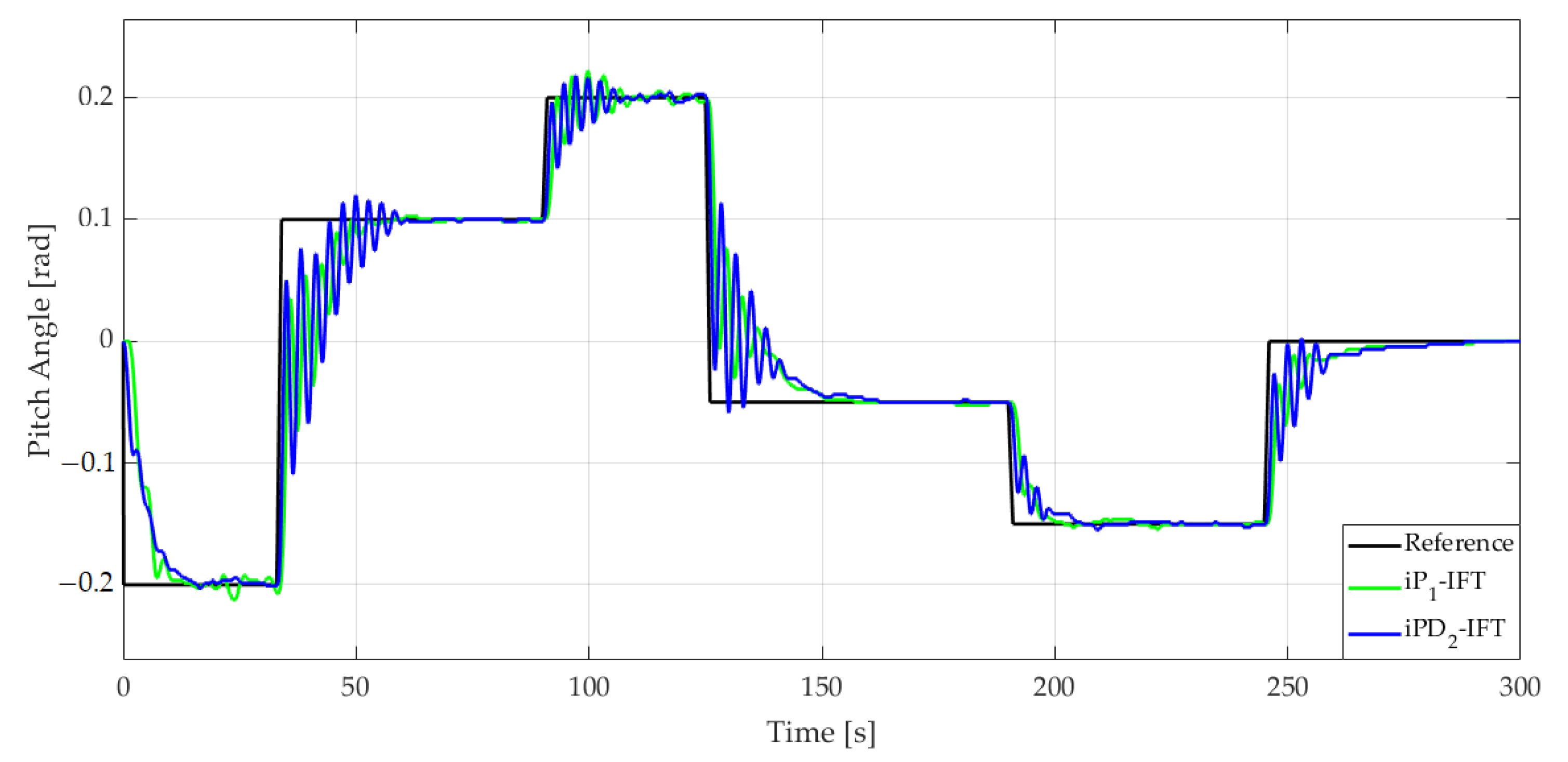
4.3. Control of Pitch Angle with iP₁-IFT and iPD₂-IFT Controllers

The controllers tuned with the IFT algorithm that were presented in Section 4.1 and Section 4.2 are used for a performance comparison with the step variations of the reference signal. The reference profile from Figure 6 used for the iP₁ comparison was considered for the experiments against the iPD₂-IFT controller. Moreover, it is necessary to analyze which type of MFC controller can offer better results for the pitch angle control of an Aero System. The results are depicted in Figure 11.

The comparison reveals a response with larger oscillations for iPD₂-IFT in relation to iP₁-IFT to the step variations of the reference signal. However, due to the derivative component, iPD₂-IFT will generate a shorter settling time. The control signals obtained from the comparative experiment are depicted in Figure 12 together with the angular speeds of the two DC motors.

The control signal of the iP₁-IFT controller is smooth compared with that of the iPD₂-IFT controller, which exhibits oscillations due to the amplification of the high-frequency signals from the control system by the derivative component. These oscillations propagate at the output of the inner loops and finally at the output of the control system, determining less satisfactory performances of the control system with iPD₂-IFT compared with those obtained using iP₁-IFT.

5. Conclusions

In this paper, a new method for tuning model-free iPID controllers based on the IFT data-driven algorithm is described. Considering that the IFT algorithm can only be used for the tuning controllers with a fixed structure, such a structure was first determined for the iPID controllers. Thus, starting from the connections between the iPID and PID discrete-time controllers, a fixed structure of the iPID controller was obtained, described by an equivalent transfer function that were parametrized with the parameters vector. Moreover, analyzing the behaviors of the iPID controllers in relation to the PID control laws, two intelligent controllers were established for $\nu =1$ and $\nu =2$, respectively, with the others being eliminated because they had unusual behaviors in the control engineering. The IFT algorithm could be applied by having the iPID controllers with a fixed structure, whose transfer functions were used to estimate the gradients of the input/output variables. At the same time, based on two experiments in the closed loop, the input and output signals were collected, which together with the above derivative estimates allowed for the estimation of the gradients of the cost function and the matrix used to update the direction. Finally, the parameters grouped in vector $\rho$ of the fixed structure of the controller were determined; based on these parameters, the tuning gains and parameter $\alpha$ were found. The methodology for tuning the iPID controllers based on the IFT algorithm was tested and experimentally validated using a real-time application for controlling the pitch angle of the dual-motor Aero 2 aerospace system, which was provided by Quanser.

The main advantages of the proposed tuning method based on the IFT algorithm consist of the following: the determination of both the gain parameters related to the PID algorithm and the α parameter; the IFT tuning of the iPID parameters does not require knowledge of the plant model; and the gradients of the quadratic control criterion can be easily estimated based on the data collected after the two experiments. Among the disadvantages, it is mentioned that the selection of the starting values of the iPID tuning parameters must be conducted in such a way so as to obtain a stable response and the two experiments must be performed to determine the tuning parameters at each step. The initial choice of tuning parameters, along with finding the related values of the step size and the penalty factor of the control effort through a trial-and-error procedure, are the main design challenges.

For future research, some techniques will be considered for tuning the parameters related to the step size and penalty factor of the control effort as well as the extending of the proposed method to multivariable systems.