Article

Application of Opposition-Based Learning Jumping Spider Optimization Algorithm in Gas Turbine Coupled Cooling System

1
School of Information Science and Engineering, Northeastern University, Shenyang 110819, China
2
China Northern Vehicle Research Institute, Beijing 100072, China
*
Author to whom correspondence should be addressed.
Actuators 2023, 12(10), 396; https://doi.org/10.3390/act12100396
Submission received: 15 September 2023 / Revised: 14 October 2023 / Accepted: 20 October 2023 / Published: 23 October 2023
(This article belongs to the Special Issue Applications of Intelligent Control in Actuators Systems)

Abstract

:
A gas turbine cooling system is a typical multivariable, strongly coupled, nonlinear system; however, the randomness and large disturbances make it difficult to control the variables precisely. In order to solve the problem of precise process control for multi-input and multi-output coupled systems with flow, pressure, and temperature, this article conducts the following research: (1) Designing a secondary circuit for waste hot water and establishing a water-circulating gas turbine cooling system to improve the efficiency of waste heat utilization. (2) Identifying the coupled system model and establishing a mathematical model of the coupling relationship based on the characteristic data of input and output signals in the gas turbine cooling system. (3) Designing a coupled-system decoupling compensator to weaken the relationships between variables, realizing the decoupling between coupled variables. (4) An Opposition-based Learning Jumping Spider Optimization Algorithm is proposed to be combined with the PID control algorithm, and the parameters of the PID controller are adjusted to solve the intelligent control problems of heat exchanger water inlet flow rate, pressure, and temperature in the gas turbine cooling system. After simulation verification, the gas turbine cooling system based on an Opposition-based Learning Jumping Spider Optimization Algorithm can realize the constant inlet flow rate, with an error of no more than 1 m3/h, constant inlet water temperature, with an error of no more than 0.2 °C, and constant main-pipe pressure, with an error of no more than 0.01 MPa. Experimental results show that a gas turbine cooling system based on the Opposition-based Learning Jumping Spider Optimization Algorithm can accurately realize the internal variable controls. At the same time, it can provide a reference for decoupling problems in strongly coupled systems, the controller parameter optimization problems, and process control problems in complex systems.

1. Introduction

Currently, high-power gas turbines with combustion efficiency exceeding 40% are widely used, and the outlet temperature of the combustion chamber usually reaches 1500 °C. The turbine impeller operates under high-pressure, high-temperature, and high-speed conditions [1]. Under the influence of sustained high temperature, thermal stress will cause deformation and cracks in the internal walls of the combustion chamber; these cracks cannot be eliminated artificially, which will eventually lead to the failure of the combustion chamber. In these circumstances, the cooling system of the gas turbine is an important link to maintain its long-term stable operation, and it is an important and hot issue in the industrial system. Gas turbine cooling systems have different structures and technologies. The gas turbine cooling system proposed by Hamed at the University of Adelaide consists of an absorption cooler, a drying rotor, and an evaporative cooler [2], the waste heat generated by the gas turbine is used to operate the absorption cooler and the drying rotor. The condensate from the absorption cooler can supply a portion of the water for the evaporative cooler. The advantages of this system are that water resources can be recycled and reused, and the limitation is that the maintenance costs are high. Samira has made efforts to improve the utilization of water resources. Firstly, the air is cooled to a dew-point temperature using M-cycle technology. Then, the absorption cooler further cools it down. Both the absorption cooler and the recirculation cooler consume very little electricity, and the source of the energy for the refrigeration and cooling of the water for recirculation comes from the waste heat of the gas turbine and the condensate of the evaporative cooler, respectively, which reduces the amount of cooling water needed for the recirculation considerably [3]. Seoul National University have designed a circulation system consisting of gas turbines, carbon dioxide turbines, and liquefied natural gas power plants. Combining the waste heat of gas turbines with the cold energy of liquefied natural gas [4]. There have been some achievements from the perspective of energy recycling, but the systems are substantial and require combined-cycle power plants, which are relatively lacking in general applicability. Barakat has combined atomized cooling systems and Exhaust Gas Recirculation to improve gas turbine performance and increase the effectiveness of its cooling system in hot and humid regions [5]. There is another kind of cooling system that uses water as coolant and realizes the cooling of components at all levels of the gas turbine through the heat transfer effect of the heat exchanger [6,7,8]. These systems are typical process control systems, and usually have more than one controlled variable such as rate of flow, pipeline pressure, and coolant temperature, etc. These variables have strong coupling, and each input interferes and interacts with the others. This phenomenon is very common in multivariable systems [9]. Decoupling techniques can realize separate control of different controlled objects through some mathematical methods or equations, weakening the connections between different variables [10]. Currently, the commonly used intelligent decoupling methods include neural network decoupling control [11], fuzzy decoupling control [12], etc. The commonly used traditional decoupling methods include feedforward compensation decoupling [13], inverted decoupling [14], diagonal matrix decoupling [15], and unit matrix decoupling. The advantages of traditional decoupling methods are simple structure, easy implementation, and significant effectiveness. Intelligent decoupling methods, including fuzzy decoupling and neural network decoupling, can achieve multi-input and multi-output mapping, approximate any function with any accuracy, and have strong self-learning functions. The decoupling control methods are summarized as shown in Table 1.
The development and application of decoupling control in multivariable industrial systems need further research and improvement because the uncertainty and randomness of a complex gas turbine cooling system have great impacts on the system in addition to the strong coupling between variables. In the middle-latitude and high-latitude regions, the temperature difference between day and night is large. There is a greater difference in temperature between different seasons. The temperature of cooling water does not even exceed 10 °C in winter. Too-low operating parameters will shorten the service life of the heat exchanger; the fluctuating inlet temperature of the heat exchanger can also affect the cooling effect. In addition, it is difficult to realize the complete decoupling of the industrial system, and the inaccuracy of system parameters or some kind of drift in operation will destroy the complete decoupling. Due to unavoidable mathematical errors in the mathematical model and decoupling compensation model, weak coupling still exists in each process channel after decoupling. This weak coupling phenomenon also affects the control effect of the system and poses a huge challenge for tuning the controller parameters of the process channel. It can be seen that the gas turbine cooling system is a typical complex process control system which is multivariable, and has strong coupling, large disturbance, and uncertainty. These complexities make it difficult to accurately tune the controller parameters of the system, which makes it difficult to accurately control the internal variables.
The tuning of the controller parameters is also an important factor affecting the system. The optimization of the controller parameters is also a typical issue in complex industrial systems. Usually, traditional control algorithms are combined with intelligent optimization algorithms to optimize controller parameters. At present, there are many kinds of mature intelligent optimization algorithms, such as Particle Swarm Optimization [24], Genetic Algorithm [25], and so on. With the development of gradually more complex industrial systems, the classical optimization algorithms have gradually exposed some limitations, such as insufficient global search ability and slow convergence speed. The optimization issue has also become a hotspot for scholars to study extensively. Both the improvement of the original algorithms and new optimization algorithms show their potential to solve many optimization problems. The advantages of population intelligence algorithms are that they can solve nonlinear, time-varying, black-box model problems in a multidimensional space. Certain behaviors of intelligent individuals can be applied to explore the optimal solution. Jumping Spider Optimization Algorithm (JSOA) is a biomimetic optimization algorithm, proposed in December 2021, which can tune a PID controller with very fine control [26]. Compared to optimization algorithms such as Coot optimization algorithm [27], Chaos game optimization [28] and Archimedes Optimization Algorithm [29], the JSOA has achieved good results in benchmark function testing of performance evaluation, with strong global search ability and fast convergence speed. However, the PID controller parameters optimized by the JSOA are not applicable to the gas turbine cooling system through simulation verification. There may be a significant deviation between the initial position of the population and the optimal position, which can result in the controller parameters not achieving the control effect of the controlled variable. In order to obtain better PID control parameters for the gas turbine cooling system, more research is needed on the mathematical expression of JSOA’s population initialization.
Intelligent population algorithms are based on “population”, using different heuristic optimization rules to search for and obtain the optimal solution. The methods of population initialization are different, including Pseudo-random Number Generators (PRNGs), Chaotic Number Generators (CNGs), Quasi-random Sequence (QRS), Uniform Design (UD), Centroidal Voronoi Tessellation (CVT), etc. [30]. At present, the initialization strategy of many optimization algorithms is the most basic PRNGs, which may not be able to obtain good results in some specific problems. It is necessary to apply more advanced population initialization strategies to more intelligent and new algorithms. In addition to PRNGs, an increasing number of initialization strategies are being developed and applied. The current research on population initialization is shown in Table 2.
Opposition-based learning is a typical multi-step algorithm [35]. Opposition-based learning calculates the fitness values of the original population and the opposite population, and uses strategies such as population merging or cross fusion to obtain a new initialized population. This strategy can effectively expand the search range, prevent falling into local optimum, and improve the effect and accuracy of simulation optimization. Opposition-based learning has been verified and applied to the Golden Jackal Optimization Algorithm [36], the Hunger Games Search Algorithm [37], and Particle Swarm Optimization [38]. With continuous development and application, the population initialization strategy based on opposition-based learning shows many advantages, but it has not been developed or applied to many new intelligent algorithms, such as the Walrus Optimization Algorithm (WaOA) [39], the Mantis Search Algorithm (MSA) [40], etc.
In order to solve the optimization problem of gas turbine cooling system controller parameters, this article decouples the strong coupling between variables through feed-forward compensation. Then, the Opposition-based Learning Jumping Spider Optimization Algorithm (Obl-JSOA) is proposed. The Obl-JSOA is applied to the PID controller-parameter tuning of gas turbine cooling system to solve the problems of long response time and difficult controller parameter tuning of gas turbine cooling system under traditional PID control. By comparing traditional PID control with PSO optimized PID control and JSOA optimized PID control, we prove that the Obl-JSOA is more suitable for gas turbine cooling systems. We establish a PID feedforward compensation decoupling control system, combining the control algorithm and intelligent algorithm, which aims to improve the control effect and control accuracy of each controlled variable in the gas turbine cooling system.

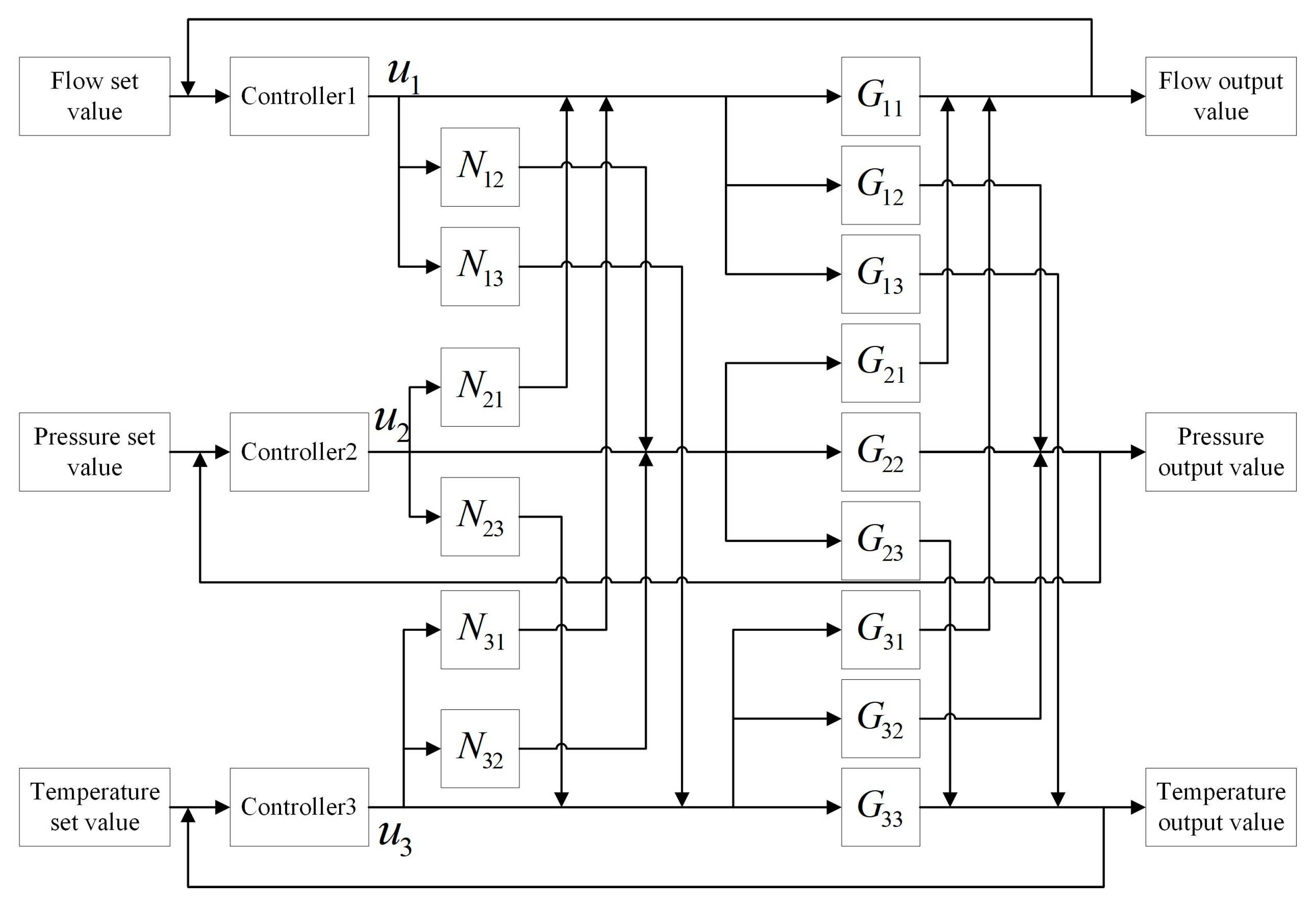
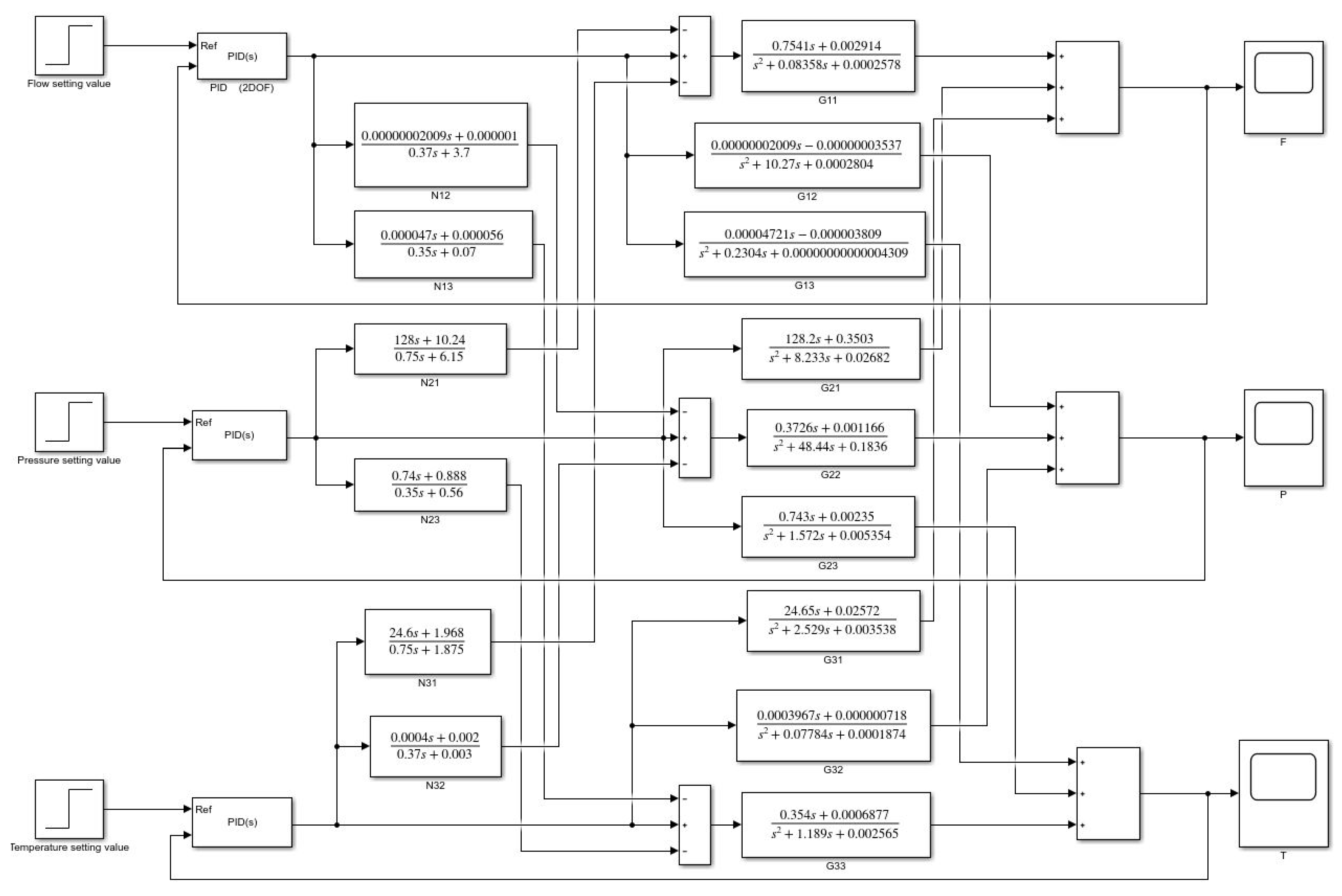
2. Gas Turbine Cooling Control System

2.1. Operating Principle and Characterization

In order to maintain the stable operation of the gas turbine and extend the service life of the heat exchanger of the cooling system, the secondary water circulation loop of the heat exchanger cooling module is designed in this section, and the waste heat of the gas turbine is used to control the cold water temperature within an appropriate range. This is because low temperatures may lead to increased wear and reduced energy efficiency, while high temperatures can affect cooling efficiency [41]. The waste hot water is mixed with the cold water input from the cold water tank, and the appropriate ratio is adjusted by controlling the valve opening and motor speed to keep the heat exchanger inlet water flow constant, the inlet water temperature constant, and the pressure of the main pipeline constant [42], so as to form a gas turbine cooling control system with constant temperature, flow, and pressure. The system structure diagram is illustrated in Figure 1.
The system consists of three main pipelines:
(1)
DN400 is a flow pipe. The flow rate of the inlet water to the heat exchanger of the cooling module (flowmeter 01 in Figure 1) is controlled by regulating the electric valve 01.
(2)
DN200 is a pressure pipe that controls the inlet water pressure ( P 1 in Figure 1) by adjusting pressure relief valve 02.
(3)
DN350 is a temperature pipe, regulating the return water flow through the pump and valve 03, which controls the inlet water temperature in the heat exchanger ( T 2 in Figure 1).
DN400 is connected to the hot tank through the heat exchanger, and the cooling water inside the pipeline consists of two parts. One is cold water in the tank, the other is the waste hot water after heat conduction with the hot tank. The constant inlet temperature of the heat exchanger is achieved by mixing cold and hot water. DN200 is the pressure relief pipe. The pipeline pressure is adjusted by changing the opening of pressure reducing valve 02. The function of the check valve is to prevent wastewater backflow. A portion of the hot water is transported to DN400 through a pump, compensating for the heat of the cold water flowing into DN400 from the tank, and realizing a constant and controllable temperature of the heat exchanger inlet water. Therefore, the inlet flow rate in the heat exchanger is affected by cold-water flow and hot-water flow, which are controlled by valve 01 and valve 03, respectively. Inlet pressure is affected by valve 01 and pressure relief valve 02. The inlet water temperature in the heat exchanger is affected by the cold water temperature, the outlet temperature of the heat exchanger, and temperature loss. Input and output characteristic curves are obtained from the experimental data of the test run as shown in Figure 2, which includes the opening of valves, pipeline pressure, flowmeter feedback, motor current feedback, etc.
Figure 2a,c are the valve opening signals, Figure 2e is the booster pump current signal, and these are the input signals of the process channel. Figure 2b,d,h are the rate of flow, pressure, and temperature signals under the action of the valve and booster pump. The signal in the figure is the data source that constitutes the three-input and three-output coupling model. We obtained the system coupling model through data source identification, providing a model basis for decoupler design. In Figure 2e,f, the current signal is enhanced and the motor speed is increased, which means that the flow rate of pipeline DN350 is increased. At this time, the opening of valve 01 is reduced and the opening of pressure relief valve 02 is increased, resulting in a decrease in cold water inflow, which maintains the balance of inflow flow. As hot water is increased and cold water is reduced, the inlet temperature of the heat exchanger gradually rises. According to the input–output relationship analysis and data curves, it can be seen that there is a strong coupling between the system variables:
F = f ( u 1 , u 2 , u 3 )
P = p ( u 1 , u 2 )
T = t ( u 1 , u 3 , T 1 , T 3 , Δ T )
where u 1 is the valve 01 opening signal, u 2 is the valve 02 opening signal, and u 3 is current signal of the booster pump in DN350. T 1 is temperature of the cold water tank, T 3 is the heat exchanger output hot water temperature, and Δ T is the pipeline temperature loss. F, P, T are DN400 electromagnetic flowmeter flow values, cold water tank outlet pressure ( P 1 ), and heat exchanger inlet temperature ( T 2 ), respectively. f, p, and t are constraint functions between variables that are difficult to express precisely. The inlet valve input temperature, temperature loss, and heat exchanger output temperature have uncertainties and the system has large value perturbations; these complexities make it difficult to control the variables precisely [43].

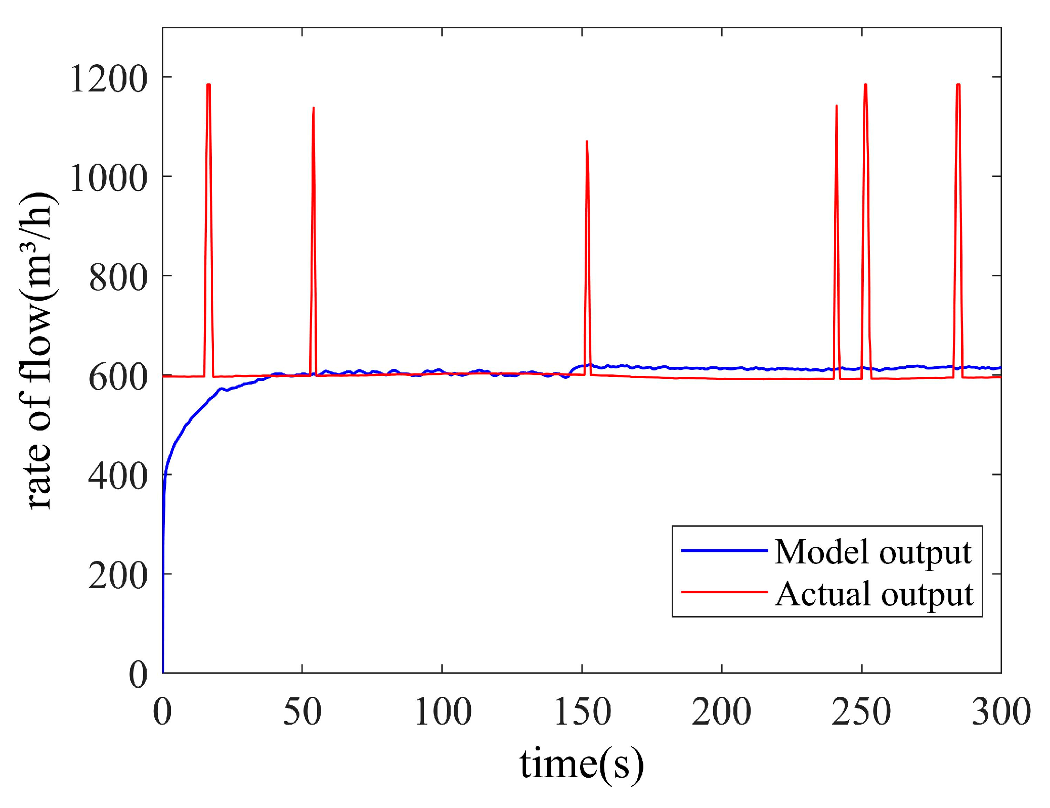
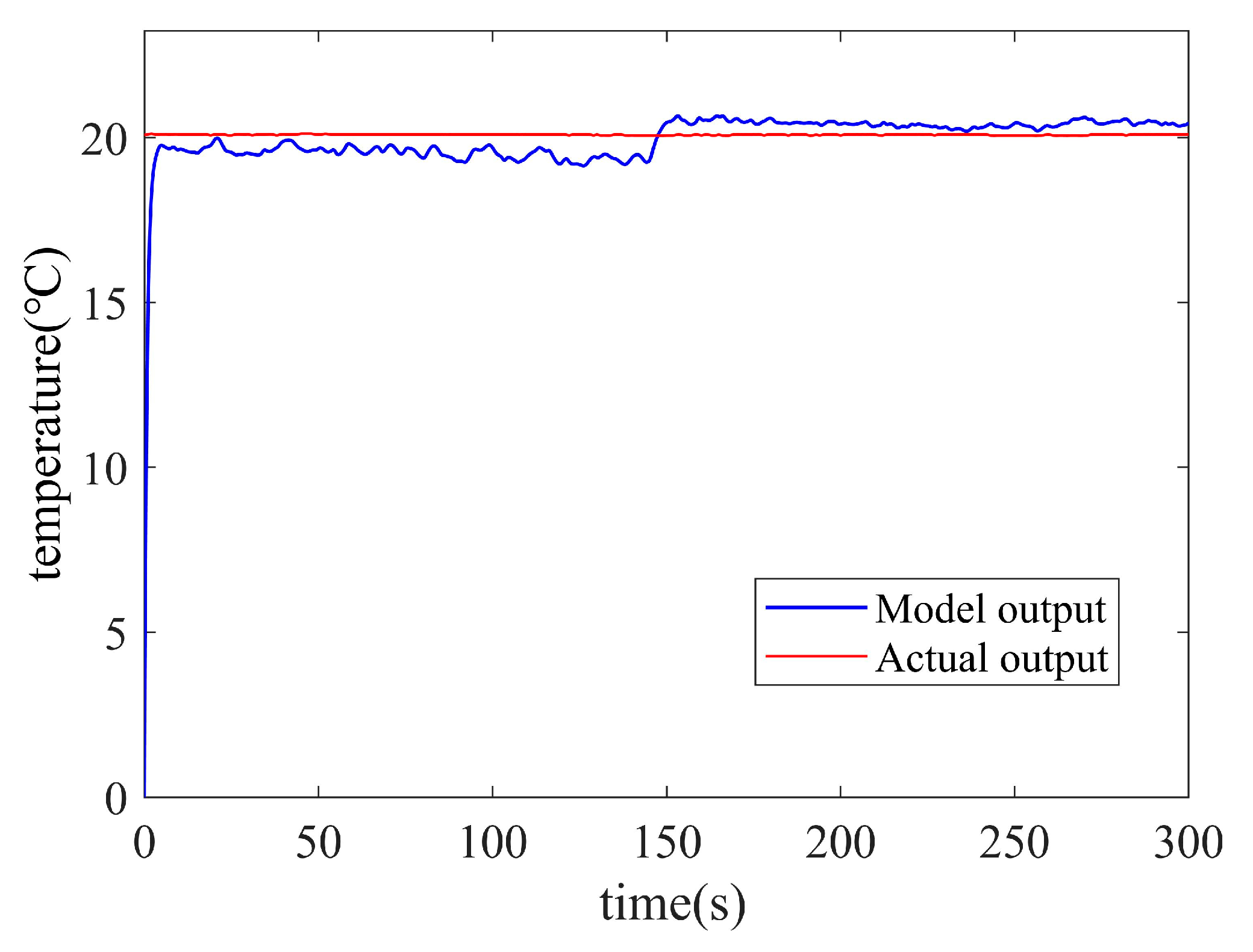
2.2. Model Identification of Coupled Gas Turbine Cooling System

According to the working principle of the system and the analysis of the coupling characteristics, it can be seen that the gas turbine cooling system has three inputs signals, which are valve 01 opening signal, pressure relief valve 02 opening signal, and the current signal of the booster pump in DN350, corresponding to the controlled objects which are the heat exchanger inlet water flow rate, pipeline pressure, and the heat exchanger inlet temperature. The block diagram of the coupling system is shown in Figure 3.
Mathematical descriptions of the inputs and outputs are obtained from the block diagram of the coupled model:
F P T = G 11 G 21 G 31 G 12 G 22 G 32 G 13 G 23 G 33 u 1 u 2 u 3
The coupled system model is obtained through the MATLAB system identification toolbox identification and the coupled model is as follows:
G 11 = 0.7541 s + 0.002914 s 2 + 0.08358 s + 0.0002578 G 12 = 2.009 e 08 s 3.537 e 08 s 2 + 10.27 s + 0.0002804 G 13 = 4.721 e 05 s 3.809 e 06 s 2 + 0.2304 s + 4.309 e 14 G 21 = 128.2 s + 0.3503 s 2 + 8.233 s + 0.02682 G 22 = 0.3726 s + 0.001166 s 2 + 48.44 s + 0.1836 G 23 = 0.743 s + 0.00235 s 2 + 1.572 s + 0.005354 G 31 = 24.65 s + 0.02572 s 2 + 2.529 s + 0.003538 G 32 = 3.967 e 04 s + 7.18 e 07 s 2 + 0.07784 s + 0.0001874 G 33 = 0.354 s + 0.0006877 s 2 + 1.189 s + 0.002565

2.3. Comprehensive Analysis of Model Error

The system transfer function model can be obtained through the system identification toolbox, providing a model basis for the subsequent design of decoupling compensators and the implementation of control over various controlled variables. This section selects 300 sets of data as the data source for establishing the mathematical model of the process control channel, and verifies the correctness of the simulation model of the three-input and three-output coupled system. Comparing the output results of the simulation model of each controlled variable with the actual on-site output results, the output results of each variable are shown in Figure 4, Figure 5 and Figure 6:
We calculated the error between model output and actual output. For the flow coupling models, the average error is 6.22%, for pressure coupled models, the average error is 3.21%, and for temperature coupled models, the average error is 5.82%. The flow output error mainly comes from the initial stage, and the maximum error after the system stabilizes is only 3.57%. The maximum error in pressure is 5.17%, but the average error does not exceed 0.01 Mpa. The maximum temperature error does not exceed 2.84%, and its main error also comes from the initial stage. The simulation model output results for each controlled variable are basically consistent with the actual output results, which can verify the correctness of the coupling model. After comprehensive error analysis, a three-input and three-output coupling system model is obtained.

2.4. Decoupling Compensator

In this section, a typical decoupling method is selected. Feedforward compensation decoupling is applied to the gas turbine cooling system. Feedforward compensation decoupling designs a compensation device, decoupling the original coupled system through the compensation device. We obtained the new transfer function after calculating the original transfer function model, and decoupling the multi-input and multi-output systems into multiple single loop systems, so as to weaken the correlation between variables. The gas turbine cooling system selects the second-order model in the model identification. There are some limitations when using other decoupling methods, which may lead to the following problems:
(1)
Diagonal matrix decoupling makes it difficult to compute the decoupling compensation matrix for a third-order MIMO system, and the matrix equation is difficult to express.
(2)
There are 27 matrix configuration cases that need to be discussed for inverted decoupling, increasing the experimental complexity, and discussing the effects and feasibility of different decoupling matrices is also complicated work.
(3)
The principle of unit matrix decoupling is similar to that of diagonal matrix decoupling, but the calculation is more difficult to realize.
The block diagram of the gas turbine cooling system feedforward compensation decoupling is shown in Figure 7.
G 11 , G 22 , and G 33 are transfer function models for flow, pressure, and temperature control, respectively. G i j (ij) are perturbations between different controlled variables. Realizing decoupling between variables needs to be satisfied:
u 1 N 12 G 22 + u 1 G 12 = 0 u 1 N 13 G 33 + u 1 G 13 = 0 u 2 N 21 G 11 + u 2 G 21 = 0 u 2 N 23 G 33 + u 2 G 23 = 0 u 3 N 31 G 11 + u 3 G 31 = 0 u 3 N 32 G 22 + u 3 G 32 = 0
The decoupling compensation model can be calculated from Equation (5) and the transfer function model:
N 12 = G 12 / G 22 N 13 = G 13 / G 33 N 21 = G 21 / G 11 N 23 = G 23 / G 33 N 31 = G 31 / G 11 N 32 = G 32 / G 22
For complex industrial systems represented by gas turbine cooling systems, it is a difficult challenge to achieve complete decoupling, and the decoupling technique is only used for better realization of accurate control of internal controlled variables. The coupled cooling system model structure is simplified by the feedforward compensation decoupling method. After adding the decoupling compensation, each variable is controlled by the positional PID control algorithm:
u ( k ) = K P e ( k ) + K I i = 0 e ( i ) + K D [ e ( k ) e ( k 1 ) ]
where e is the error between the set and measured values of flow, pressure, and temperature of the controlled variables for the gas turbine cooling system. The gas turbine cooling system decoupling control simulation is shown in Figure 8.
The parameters of the PID controller are adjusted empirically. The results of flow, pressure and temperature control are shown in Figure 9.
The control objective of the gas turbine cooling system is to maintain a constant inlet flow rate of the heat exchanger, with a target set value of 600 m3/h and an error of no more than 5 m3/h; the inlet temperature of the heat exchanger is constant, with a target setting of 22 °C and an error of no more than 0.2 °C; the maximum temperature overshoot is less than 2 °C; the pressure of the main pipeline is constant, not exceeding 0.3 MPa. After decoupling compensation, although each controlled variable can be controlled within the technical indicators, some problems, such as long adjustment time and reliance on staff experience, can reduce production efficiency.

3. Opposition-Based Learning Jumping Spider Optimization Algorithm

3.1. Opposition-Based Learning Population Initialization Strategy

Opposition-based learning is based on individual fitness values, mixing and modifying population individuals to form a new initial population. Opposition-based learning population initialization involves three steps:
(1)
Generating an original population. The original population is a pseudo-random number generated by a random algorithm, which can be either PRNGs or CNGs.
(2)
Generating an oppositive population of the same size according to a heuristic rule. The heuristic rule is:
x o b l = upper _ bound + lower _ bound x o r i
x o b l is individual position of oppositive population, upper_ Bound is the upper bound of the feasible region of the initial solution, lower_ Bound is the lower bound of the feasible region of the initial solution, and x o r i is the original population generated by PRNGs.
(3)
Selecting the appropriate individual as the new population based on the calculated individual fitness value. An opposition-based learning population initialization flowchart is shown in Figure 10:
Opposition-based learning population initialization utilizes fitness values to optimize the individual positions of the population during the population initialization stage. For heuristic algorithms, the distance between the individual positions of the population and the optimal individual position determines the convergence speed of the algorithm. If the individual positions are closer to the optimal position, the convergence speed of the individual population will be significantly improved during calculation. If PRNGs are used to generate purely random individuals, the convergence speed cannot be predicted. An opposition-based learning strategy analyzes the position of each individual and the position of an opposition-based individual, calculates the fitness value, and categorizes individuals with more suitable fitness into the final population, forming the final population, and then performs optimization iterations.

3.2. Principles of Obl-JSOA

The JSOA is a new heuristic population algorithm, which has good performance in benchmark function tests. However, the population initialization strategy of the JSOA has not been studied and other forms of mathematical representations have not been fully developed. This section applies the opposition-based learning strategy to the JSOA and an opposition-based Learning Jumping Spider Optimization Algorithm is proposed, which is applied to optimize the parameter tuning of the PID controller of a gas turbine cooling system. The steps of the Obl-JSOA tuning PID controller are as follows:
(1)
Defining the number of populations and the maximum number of iterations, which are set to 50 and 30, respectively. PRNGs are used to randomly generate the locations of individual jumping spiders and then a population of opposition-based jumping spiders is generated according to the opposition-based learning heuristic rule.
(2)
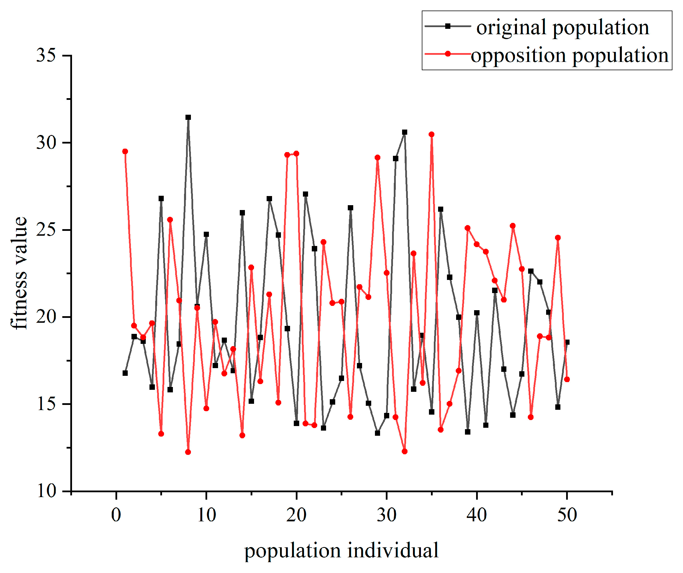
The sum of the relative error of each controlled variable and the output standard deviation is used as the fitness function to calculate the individual fitness values of the original population and opposition population. In the union of the original population and the opposing population (100 individuals), 50 individuals with better fitness values are selected as the new original population to complete the population initialization of the opposition-based learning strategy, and the fitness values of the original and opposition-based populations are shown in Figure 11.
If the 50 individuals with the smallest fitness values are chosen as the initial population, it can greatly improve the convergence speed, but it is equally easy to converge prematurely and fall into the local optimal solution. In order to balance the convergence of the algorithm and the global search ability, the pseudo-code for the new population is determined as follows:
Opposition-based Learning population initialization strategy
1.    Initializing population pop through pseudo-random number generators
2.    Calculating fitness value ori_fitness
3.    Generating opposition-based population obl_pop bt Equation (3)
4.    Calculating opposition-based population fitness value obl_fitness
5.    For i = 1: SearchAgents
6.    If obl_fitness(i) < ori_fitness(i)
7.    pop(i) = obl_pop(i)
8.    orifitness(i) = oblfitness(i)
9.    End if
10.  End for
11.  Return pop and orifitness
12.  Ending procedure
(3)
Iterative optimization: each iteration updates the individual positions according to the algorithmic optimization strategy (persecution strategy, jumping strategy, etc.), which in turn updates the parameters of the PID controller.
(4)
Calculating the pheromone concentration based on the individual fitness value, and determining whether the current individual needs to update its position according to the pheromone model discrimination condition.
(5)
Updating the position of the best individual in the recorded population and the best fitness value until the completion of the iteration, and transporting the optimal PID controller parameters into the simulink model through the sim function.
There are some things that need special attention:
JSOA is a meta-heuristic algorithm that requires problem features when solving practical problems. Both Pseudo-random Number Generators and opposition-based learning require prior knowledge. To put it another way, if the controller parameters or some other parameters that need to be optimized are completely unknown, the Obl-JSOA may produce poor results. The individual positions generated by PRNGs are not guided by prior knowledge or fitness values, which may result in no competitiveness and complete substitution by opposing populations. This circumstance can lead to the algorithm falling into a local optimal solution, and the obtained parameters are not suitable for the control system. If there is a lack of prior knowledge and it is uncertain whether it is beneficial for the system, it is not recommended to directly introduce an opposition-based learning strategy.
The Obl-JSOA flowchart is shown in Figure 12.

4. Simulation Results of the Gas Turbine Cooling Control System

After completing the system model establishment, decoupling compensator establishment, control algorithm, and optimization algorithm design, simulation experiments are carried out with the following steps:
(1)
Establishing a simulation model of the gas turbine cooling system and setting the parameters of the PID controller as variables, which are represented as the position of individual jumping spiders in the Obl-JSOA.
(2)
Using an opposition-based learning strategy to initialize the individual positions of the population in order to initialize the PID controller parameters.
(3)
Iterative calculation: updating individual positions according to algorithm optimization strategies for each iteration, and then updating the parameters of the PID controller.
In this section, traditional PID control, PSO optimized PID control, JSOA optimized PID control, and Obl-JSOA optimized PID control are compared. In order to make the results more intuitive, the rise time, systematical errors, and overshoot are selected as the performance indexes, and a comparison of flow, pressure, and temperature control effects on the gas turbine cooling control system is shown in Figure 13, Figure 14 and Figure 15:
The technical indicators of the gas turbine cooling system are as follows: the rate of flow is 600 m3/h, and the error does not exceed 5 m3/h; the pressure remains constant at 0.3 MPa, with an error not exceeding 0.01 Mpa; the inlet temperature of the heat exchanger remains constant at 22 °C, with an error of no more than 0.2 °C, and the maximum overshoot does not exceed 2 °C. The data from the test run shows that the cold water temperature in the water tank does not exceed 20 °C. It takes almost 30 min to increase the inlet temperature of the original coupling system to 22 °C without affecting the flow rate and pressure. After adjustment using the PID controller and decoupling compensator, it also takes 50 s. The combination of the Obl-JSOA and the PID control algorithm greatly accelerates the adjustment time of the controlled variable and improves the control effect.
As shown in Figure 2f, the current signal of the booster pump increases, and the return water flow rate of the DN350 pipeline increases. At the same time, the opening of valve 01 decreases, while the opening of pressure relief valve 02 increases, as shown in Figure 2a,c, maintaining a constant inlet flow rate in the heat exchanger. Due to an increase in circuit water and a decrease in inlet water, the inlet water temperature of the heat exchanger gradually increases. Finally, each controlled variable reaches the set value. Accurate control of controlled variables in the gas turbine cooling system has been achieved.
In addition, there are some explanations that have to be mentioned:
(1)
Whether in simulation or experiment, there may be situations where the pressure exceeds 0.3 MPa. The system can accept it as long as it does not seriously exceed 0.3 MPa for a long time, as the strength and toughness of pipeline materials are usually high.
(2)
Plate heat exchangers and pipelines both dissipate heat towards the surrounding environment, and the flow rate and heat transfer coefficient are not constant. The temperature will not rise this fast in actual experiments.
(3)
The coupling model is established based on on-site input and output signals, and there are significant disturbances that result in inaccurate transfer function models describing the system. There is an error between the model pressure output result and the actual pressure output result. If the coupling between pressure and other variables is strong, the existing error can lead to poor control effects, and even overload pressure.
The rise times, systematical errors, and overshoots for the four methods are shown in Table 3, Table 4 and Table 5.
We performed performance testing on the optimized intelligent system of the Obl-JSOA. Disturbance is added to flow control at 5 s, and pressure and temperature control at 20 s. The control effects of each variable after adding disturbances are shown in Figure 16, Figure 17 and Figure 18.
As shown in the figures, the rate of flow, pressure, and temperature are significantly disturbed at 5 s and 20 s, respectively. The loop that controls rate of flow has strong stability and returns to normal indicators within 1 s. The loop that controls the pressure returns to normal indicators after 2 s. In fact, although the actual system has strict pressure requirements, the internal pressure of the pipeline is within the technical indicators during simulation and experiments, and generally does not exceed the set range. The loop that controls the temperature returns to normal indicators after 5 s. When there is disturbance in the system, it can return to normal indicators after a short period of adjustment.
From the figures and tables, it can be seen that when an Obl-JSOA is applied to optimize the PID controller parameters of the gas turbine cooling system, the rise time and overshoot are significantly reduced. For flow control, compared to PID control, all three indicators have been significantly improved. Compared to other optimization algorithms, the Obl-JSOA has a faster rise time and does not generate overshoot. For pressure control, the maximum overshoot does not exceed 0.01 Mpa, and rise time and systematical errors are reduced. For temperature control, although the overshoot generated by the Obl-JSOA is greater than other methods, it has a shorter rise time and faster adjustment time. In fact, the overshoot is only 0.81%, not exceeding 0.2 °C. Significantly reducing the adjustment time within other technical indicators can also demonstrate the superiority of the Obl-JSOA. Through simulation verification, compared with other algorithms, the obtained PID controller parameters of the Obl-JSOA are more suitable for gas turbine cooling systems.

5. Conclusions

There is strong coupling and randomness between variables in a gas turbine cooling system, which makes it difficult to accurately control the controlled variables. The combination of intelligent algorithms and control algorithms aims to improve the system control effect. When tuning PID controller parameters with intelligent algorithms, due to insufficient prior knowledge, the optimized PID controller parameters are not suitable for gas turbine cooling systems, and there are still problems such as systematical errors, overshoots, and long adjustment times. This article proposes an Obl-JSOA for parameter tuning of PID controllers in gas turbine cooling systems. By integrating an opposition-based learning strategy based on individual fitness values, the population individuals are mixed and modified to form a new initial population, enabling the algorithm to obtain better prior knowledge and improving the effectiveness and accuracy of simulation optimization. The experimental results show that PID controller parameters optimized by Obl-JSOA with the fusion of opposition-based learning strategy are more suitable for multivariable complex systems such as gas turbine cooling systems. Compared with the JSOA, the adjustment times for flow, pressure, and temperature of the Obl-JSOA have been accelerated by 0.48 s, 5.09 s and 47.56 s, respectively. Compared with traditional PID, the systematic errors of flow, pressure, and temperature have been reduced by 0.05%, 0.44%, and 0.32%. The overshoot of flow and pressure has been reduced by 2.35% and 4.5%. The designed gas turbine cooling system can improve the service life of the heat exchanger. In addition, the combination of an opposition-based learning strategy, an intelligent algorithm, and a control algorithm also provides transplantation and reference significance for other complex process control systems.

Author Contributions

Conceptualization, D.W., T.L., Y.N. and K.S.; methodology, D.W., T.L., Y.N. and Y.L.; software, D.W., T.L. and Y.L.; validation, D.W., T.L., Y.N., Y.L. and K.S.; formal analysis, D.W.; investigation, D.W., T.L., Y.N., Y.L. and K.S.; resources, D.W., T.L., Y.N. and K.S.; data curation, D.W. and T.L.; writing—original draft preparation, D.W., T.L., Y.L. and K.S.; supervision, D.W. All authors have read and agreed to the published version of the manuscript.

Funding

This research was funded by National Natural Science Foundation of China (Grant number 52077027), and the Department of Science and Technology of Liaoning province (Grant number 2020020304-JH1/101).

Data Availability Statement

Not applicable.

Conflicts of Interest

The authors declare no conflict of interest.

References

  1. Unnikrishnan, U.; Yang, V. A review of cooling technologies for high temperature rotating components in gas turbine. Propuls. Power Res. 2022, 11, 293–310. [Google Scholar] [CrossRef]
  2. Hamed, S.D.; Eric, J.H.; Lei, C.; Samira, P. Using novel integrated Maisotsenko cooler and absorption chiller for cooling of gas turbine inlet air. Energy Convers. Manag. 2019, 195, 1067–1078. [Google Scholar]
  3. Samira, P.; Eric, J.H.; Lei, C. Simulation of innovative hybridizing M-cycle cooler and absorption-refrigeration for pre-cooling of gas turbine intake air: Including a case study for Siemens SGT-750 gas turbine. Energy 2022, 247, 123356. [Google Scholar]
  4. Cha, S.H.; Na, S.I.; Lee, Y.H.; Kim, M.S. Thermodynamic analysis of a gas turbine inlet air cooling and recovering system in gas turbine and CO2 combined cycle using cold energy from LNG terminal. Energy Convers. Manag. 2021, 230, 113802. [Google Scholar] [CrossRef]
  5. Barakat, E.; Jin, T.; Wang, G.F. Performance analysis of selective exhaust gas recirculation integrated with fogging cooling system for gas turbine power plants. Energy 2023, 263, 125849. [Google Scholar] [CrossRef]
  6. Abdul Karim, Z.A.; Mohd Azmi, M.N.H.; Abdullah, A.S. Design of a Heat Exchanger for Gas Turbine Inlet Air using Chilled Water System. Energy Procedia 2012, 14, 1689–1694. [Google Scholar] [CrossRef]
  7. Baina, F.; Malmquist, A.; Alejo, L.; Palm, B.; Fransson, T.H. Analysis of a high-temperature heat exchanger for an externally-fired micro gas turbine. Appl. Therm. Eng. 2015, 75, 410–420. [Google Scholar] [CrossRef]
  8. Xu, J.; Wang, R.; Zhang, Q.X.; Cui, T.; Li, H.; Pei, L.; Quan, X.R. Design of Engine Cooling System Using Improved Particle Swarm Optimization Algorithm. IEEE Sens. J. 2023, 23, 19060–19072. [Google Scholar] [CrossRef]
  9. Liu, L.; Tian, S.; Xue, D.Y.; Tao, Z.; Chen, Y.Q.; Zhang, S. A Review of Industrial MIMO Decoupling Control. Int. J. Control. Autom. Syst. 2019, 17, 1246–1254. [Google Scholar] [CrossRef]
  10. Hägglund, T.; Shinde, S.; Theorin, A.; Thomsen, U. An industrial control loop decoupler for process control applications. Control Eng. Pract. 2022, 123, 105138. [Google Scholar] [CrossRef]
  11. Wang, C.Y.; Zhao, W.Z.; Luan, Z.K.; Gao, Q.; Deng, K. Decoupling control of vehicle chassis system based on neural network inverse system. Mech. Syst. Signal Process. 2018, 106, 176–197. [Google Scholar] [CrossRef]
  12. Zhao, D.D.; Xia, L.; Dang, H.B.; Wu, Z.Z.; Li, H.Y. Design and control of air supply system for PEMFC UAV based on dynamic decoupling strategy. Energy Convers. Manag. 2022, 253, 115159. [Google Scholar] [CrossRef]
  13. Skogestad, S.; Zotică, C.; Alsop, N. Transformed inputs for linearization, decoupling and feedforward control. J. Process Control 2023, 122, 113–133. [Google Scholar] [CrossRef]
  14. Luan, X.L.; Chen, Q.; Albertos, P.; Liu, F. Compensator design based on inverted decoupling for non-square processes. IET Control Theory Appl. 2017, 11, 996–1005. [Google Scholar] [CrossRef]
  15. Kunimatsu, S.; Tateishi, K.; Ishitobi, M.; Fujii, T. Optimal decentralized servo control for systems with diagonal decoupling matrix. IFAC Proc. Vol. 2011, 44, 2558–2563. [Google Scholar] [CrossRef]
  16. Gong, D.W.; Qiu, Z.Q.; Zheng, W.; Ke, Z.W.; Liu, Y. Intelligent Decoupling Control Study of PMSM Based on the Neural Network Inverse System. Front. Energy Res. 2022, 10, 936776. [Google Scholar]
  17. Zhang, Y.; Luan, T.; Yao, Y. MtsPSO-PID Neural Network Decoupling Control in Power Plant Boiler. IFAC Proc. Vol. 2013, 46, 101–105. [Google Scholar] [CrossRef]
  18. Liao, Q.L.; Sun, D. Sparse and decoupling control strategies based on Takagi–Sugeno fuzzy models. IEEE Trans. Cybern. 2019, 51, 947–960. [Google Scholar] [CrossRef]
  19. Londhe, P.S.; Mohan, S.; Patre, B.M.; Waghmare, L.M. Robust task-space control of an autonomous underwater vehicle-manipulator system by PID-like fuzzy control scheme with disturbance estimator. Ocean Eng. 2017, 139, 1–13. [Google Scholar] [CrossRef]
  20. Liu, Z.; Chen, H.C.; Peng, L.; Ye, X.C.; Xu, S.C.; Zhang, T. Feedforward-decoupled closed-loop fuzzy proportion-integral-derivative control of air supply system of proton exchange membrane fuel cell. Energy 2022, 240, 122490. [Google Scholar] [CrossRef]
  21. Garrido, J.; Vázquez, F.; Morilla, F. Inverted decoupling internal model control for square stable multivariable time delay systems. J. Process Control 2014, 24, 1710–1719. [Google Scholar] [CrossRef]
  22. Garrido, J.; Vázquez, F.; Morilla, F. An extended approach of inverted decoupling. J. Process Control 2011, 21, 55–68. [Google Scholar] [CrossRef]
  23. Wen, S.; Wang, J.S.; Gao, X.P.; Fang, X.H. Water lever decoupling control strategy and simulation experiments of high pressure heating system. In Proceedings of the 2018 Chinese Control and Decision Conference (CCDC), Shenyang, China, 9–11 June 2018; Volume 9, p. 11. [Google Scholar]
  24. Mirjalili, S.; Dong, J.S.; Lewis, A.; Sadiq, A.S. Particle Swarm Optimization: Theory, Literature Review, and Application in Airfoil Design. Nat. Inspired Optim. 2020, 811, 167–184. [Google Scholar]
  25. Katoch, S.; Chauhan, S.S.; Kumar, V. A review on genetic algorithm: Past, present, and future. Multimed. Tools Appl. 2021, 80, 8091–8126. [Google Scholar] [CrossRef]
  26. Peraza-Vázquez, H.; Peña-Delgado, A.F.; Ranjan, P.; Barde, C.; Choubey, A.; Morales-Cepeda, A.B. A Bio-Inspired Method for Mathematical Optimization Inspired by Arachnida Salticidade. Mathematics 2022, 10, 102. [Google Scholar] [CrossRef]
  27. Naruei, I.; Keynia, F. A new optimization method based on COOT bird natural life model. Expert Syst. Appl. 2021, 183, 115352. [Google Scholar] [CrossRef]
  28. Talatahari, S.; Azizi, M. Optimization of constrained mathematical and engineering design problems using chaos game optimization. Comput. Ind. Eng. 2020, 145, 106560. [Google Scholar] [CrossRef]
  29. Hashim, F.A.; Hussain, K.; Houssein, E.H.; Mabrouk, M.S.; Al-Atabany, W. Archimedes optimization algorithm: A new metaheuristic algorithm for solving optimization problems. Appl. Intell. 2021, 51, 1531–1551. [Google Scholar] [CrossRef]
  30. Kazimipour, B.; Li, X.; Qin, A.K. A review of population initialization techniques for evolutionary algorithms. In Proceedings of the 2014 IEEE Congress on Evolutionary Computation (CEC), Beijing, China, 6–11 July 2014; pp. 2585–2592. [Google Scholar]
  31. Pant, M.; Thangaraj, R.; Abraham, A. Particle Swarm Optimization: Performance Tuning and Empirical Analysis. In Foundations of Computational Intelligence; Abraham, A., Hassanien, A.E., Siarry, P., Engelbrecht, A., Eds.; Springer: Heidelberg, Germany, 2009; Volume 3, pp. 101–128. [Google Scholar]
  32. Zhang, M.; Zhang, W.; Sun, Y. Chaotic co-evolutionary algorithm based on differential evolution and particle swarm optimization. In Proceedings of the 2009 IEEE International Conference on Automation and Logistics, Shenyang, China, 5–7 August 2009. [Google Scholar]
  33. William, J.M.; Russel, E.C. Quasi-Random Sequences and Their Discrepancies. SIAM J. Sci. Comput. 1994, 15, 1251–1279. [Google Scholar]
  34. Kazimipour, B.; Li, X.; Qin, A. Initialization methods for large scale global optimization. In Proceedings of the Evolutionary Computation (CEC), Cancun, Mexico, 20–23 June 2013; pp. 2750–2757. [Google Scholar]
  35. Li, J.H.; Gao, Y.L.; Wang, K.G.; Sun, Y. A dual opposition-based learning for differential evolution with protective mechanism for engineering optimization problems. Appl. Soft Comput. 2021, 113, 107942. [Google Scholar] [CrossRef]
  36. Mohapatra, S.; Mohapatra, P. Fast random opposition-based learning Golden Jackal Optimization algorithm. Knowl. -Based Syst. 2023, 275, 110679. [Google Scholar] [CrossRef]
  37. Luo, X.L.; Du, B.; Gui, P.; Zhang, D.Y.; Hu, W. A Hunger Games Search algorithm with opposition-based learning for solving multimodal medical image registration. Neurocomputing 2023, 540, 126204. [Google Scholar] [CrossRef]
  38. Jiao, J.J.; Cheng, J.L.; Liu, Y.B.; Yang, H.Y.; Tan, D.R.; Cheng, P.; Zhang, Y.Q.; Jiang, C.L.; Chen, Z. Inversion of TEM measurement data via a quantum particle swarm optimization algorithm with the elite opposition-based learning strategy. Comput. Geosci. 2023, 174, 105334. [Google Scholar] [CrossRef]
  39. Trojovský, P.; Dehghani, M. A new bio-inspired metaheuristic algorithm for solving optimization problems based on walruses behavior. Sci. Rep. 2023, 13, 8775. [Google Scholar] [CrossRef]
  40. Mohamed, A.B.; Mohamed, R.; Zidan, M.; Mohamed, J.; Mohamed, A. Mantis Search Algorithm: A novel bio-inspired algorithm for global optimization and engineering design problems. Comput. Methods Appl. Mech. Eng. 2023, 415, 116200. [Google Scholar]
  41. Pilkington, A.; Rosic, B.; Tanimoto, K.; Horie, S. Prediction of natural convection heat transfer in gas turbines. Int. J. Heat Mass Transf. 2019, 141, 233–244. [Google Scholar] [CrossRef]
  42. Padovani, D.; Rundo, M.; Altare, G. The Working Hydraulics of Valve-Controlled Mobile Machines: Classification and Review. J. Dyn. Syst. Meas. Control 2020, 142, 070801. [Google Scholar] [CrossRef]
  43. Wang, S.H.; Tian, Y.T.; Li, S.J. A simultaneous optimization of a flexible heat exchanger network under uncertain conditions. Appl. Therm. Eng. 2021, 183, 116230. [Google Scholar] [CrossRef]
Figure 1. Gas turbine cooling system structure.
Actuators 12 00396 g001
Figure 2. Data characterization curve; (a) DN400 valve position feedback; (b) DN400 flow meter feedback; (c) DN200 valve position feedback; (d) cold water tank outlet pressure; (e) DN350 booster pump current feedback; (f) DN350 booster pump speed feedback; (g) cold water tank inlet temperature; and (h) heat exchanger inlet water temperature.
Actuators 12 00396 g002aActuators 12 00396 g002b
Figure 3. Block diagram of cooling system coupling model.
Actuators 12 00396 g003
Figure 4. Rate of flow output results.
Actuators 12 00396 g004
Figure 5. Pressure output results.
Actuators 12 00396 g005
Figure 6. Temperature output results.
Actuators 12 00396 g006
Figure 7. Feedforward decoupling block diagram.
Actuators 12 00396 g007
Figure 8. Simulation diagram of decoupled control of gas turbine cooling system.
Actuators 12 00396 g008
Figure 9. PID control results: (a) flow control; (b) pressure control; (c) temperature control.
Actuators 12 00396 g009
Figure 10. Opposition-based learning population initialization flowchart.
Actuators 12 00396 g010
Figure 11. Value of population fitness.
Actuators 12 00396 g011
Figure 12. Obl-JSOA flowchart.
Actuators 12 00396 g012
Figure 13. Flow control results.
Actuators 12 00396 g013
Figure 14. Pressure control results.
Actuators 12 00396 g014
Figure 15. Temperature control results.
Actuators 12 00396 g015
Figure 16. Rate of flow control performance test.
Actuators 12 00396 g016
Figure 17. Pressure control performance test.
Actuators 12 00396 g017
Figure 18. Temperature control performance test.
Actuators 12 00396 g018
Table 1. A review of decoupling methods.
Decoupling MethodsAdvantagesDrawbacks
neural network decouplingLow requirement of mathematical models [16]It is easy for the weight learning of neural network to fall into local optimum [17]
fuzzy decouplingThe establishment of corresponding fuzzy rules can solve the coupled system with no clear mapping relationship [18]It has more parameters to set, making it difficult to formulate fuzzy rules [19]
feedforward compensation decouplingThe general expression of the model is easier to obtain and implement [20]Depend on process channel characteristics, require high model accuracy
inverted decouplingDecoupled models are easy to express and less computationally difficult [21]There are too many results from decoupling matrices of multidimensional systems [22].
diagonal matrix decouplingTransforming MIMO systems into multiple complementary single loop systems [23]Transfer function models for complex industrial systems are complex and difficult to compute
unit matrix decouplingDecoupling significantly improves system performanceCompletely dependent on process dynamics, difficult to apply in engineering
Table 2. A review of population initialization techniques for intelligence algorithms.
Population Initialization TechniquesAdvantagesDrawbacks
PRNGsThe most commonly
used population initializers [31]
PRNGs cannot produce perfect evenly distributed points
CNGsRandomness and regularity are desirable [32]It can
hardly be generalized to higher dimensions
QRSQRS techniques have strong theoretical advantages over stochasticPopulation size is relatively smaller than it
should be to satisfy the underlying assumptions [33]
UDUD is directly applicable to nominal and discrete
optimization problems
High cost of assessing and counting stocks [34]
CVTProducing geometrically uniform populations without
using any objective function evaluations
The performance of the algorithm depends on the internal zoning or distance metric, introducing additional parameters
Table 3. Rise times.
VariableObl-JSOAJSOAPSOPID
Flow0.09 s0.13 s0.23 s0.57 s
Pressure0.46 s0.88 s0.98 s5.55 s
Temperature1.58 s2.13 s5.53 s49.14 s
Table 4. Systematic errors.
VariableObl-JSOAJSOAPSOPID
Flow0%0%0%0.05%
Pressure0.03%0.067%0.067%0.47%
Temperature0%0%0.045%0.32%
Table 5. Overshoots.
VariableObl-JSOAJSOAPSOPID
Flow0%0%0%2.35%
Pressure1.8%3.07%2.7%6.3%
Temperature0.81%0.77%0%0%
Disclaimer/Publisher’s Note: The statements, opinions and data contained in all publications are solely those of the individual author(s) and contributor(s) and not of MDPI and/or the editor(s). MDPI and/or the editor(s) disclaim responsibility for any injury to people or property resulting from any ideas, methods, instructions or products referred to in the content.

