Design of an Improved Active Disturbance Rejection Control Method for a Direct-Drive Gearshift System Equipped with Electromagnetic Linear Actuators in a Motor-Transmission Coupled Drive System

Abstract

In this study, a type of direct-drive gearshift system integrated into a motor-transmission coupled drive system is introduced. It used two electromagnetic linear actuators (ELAs) to perform gearshift events. The adoption of ELAs simplifies the architecture of the gearshift system and has the potential to further optimize gearshift performance. However, a number of nonlinearities in the gearshift system should be investigated in order to enhance the performance of the direct-drive gearshift system. An active disturbance rejection control (ADRC) method was selected as the principal shifting control method due to the simple methodology and strong reliability. The nonlinear characteristics of the electromagnetic force produced by the ELA were subsequently reduced using the inverse system method (ISM) technique. The ADRC approach also incorporated an acceleration feedforward module to enhance the precision of displacement control. The extended state observer (ESO) module used a nonlinear function in place of the original function to improve the ability to reject disturbances. Comparative simulations and experiments were carried out between the ADRC method and improved ADRC (IADRC) method. The outcomes demonstrate the effectiveness of the designed control method. The shift force fluctuates less, and the shift jerk decreases noticeably during the synchronization procedure. In conclusion, combined with the optimized IADRC method, the direct-drive gearshift system equipped with ELAs shows remarkable gearshift performance, and it has the potential to be widely used in motor−transmission coupled drive systems for EVs.

1. Introduction

The electromagnetic linear actuator (ELA) can output linear movement without any intermediate motion converter mechanism such as gearings. Because of this, it can directly drive the controlled objects, which is usually known as direct−drive technology. Less components, quicker dynamic performance, improved driving efficiency, and reliability are some benefits of using direct−drive technology. Hence, the direct−drive technology is widely applied recently in robotics, machine tools, wind electricity and wheel drive of electric vehicles [1,2,3,4]. ELA is one of the most important components of the direct−drive system. Recent studies focus on several areas, including parametrization structure design [5,6], precise motion control [7,8] and elimination of nonlinear disturbance [9,10].

Additionally, the ELAs’ application fields now include the automotive industry area. In the reference [11], a fully variable valve system for a high−performance engine was built using ELAs. Li adopted linear motors as the actuating device of an electromagnetic active suspension system [12]. In order to obtain high precision servo control, Li created a sort of direct−drive−type AMT equipped with ELAs and investigated the servo dynamic stiffness of the ELAs [8,13]. The authors also employed two ELAs to actuate the gearshift events of automated manual transmission (AMT) in reference [14]. However, there is no discussion of the precise displacement control in the shifting process that takes nonlinearities and disturbances into account.

The applications of ELAs in AMT gearshift systems are explored in references [13] and [14], especially for electric vehicles (EVs). The reason for this is that multi−speed transmission−equipped EVs are considered as an appropriate and competitive solution for extended−range EVs and can also can enhance the EVs’ capacity for accelerating and climbing. In addition, the size and cost of the driving motor for the can be reduced with the use of multi−speed transmission.

In comparison to other types of transmission such as automatic transmission, continuous variable transmission and dual clutch transmission, AMT has a superior dynamic performance, a simpler structure, and lower cost. Therefore, researchers prefer to integrate driving motors with AMT to extend the driving range for EVs. Power interruption problems during the gearshift process are one of the most fatal drawbacks of AMT. However, the capacity of the electric motor to quickly change its rotational speed and torque is useful to reduce the impact of power interruption on the gearshift performance. In order to minimize the rotational speed difference that must be synchronized during the gearshift process, the driving motor rotational speed is swiftly adjusted to the desired value. As a result, the power interruption time, which also serves as the gearshift time, noticeably decreases. The rotational speed difference can typically be minimized to 50−300 r/min depending on the operating conditions.

The applications of AMT in EVs and HEVs have been widely investigated. Experimental and theoretical studies on coordinated control of AMT and driving motor, structural innovation and control parameters optimization of passenger cars have been conducted more frequently recently. In reference [15,16], additional power delivery paths were attempted in an effort to structurally innovate a solution to the torque interruption problem. In reference [15], a brand-new dual input multi−speed AMT was designed for electric cars in order to implement power−on shifting. A low−speed driving motor was employed as the assisting motor installed on the final shaft to supply power during the gearshift process. A high−speed driving motor was used as the primary power source that directly linked to AMT. Song et al. develop a kind of seamless two-speed AMT. It consisted of a single planetary gear system, a disk friction clutch and a drum brake. According to simulation and test data, the transmission considerably increased the electric motor efficiency, vehicle dynamics, and energy consumption [16]. It also completely eliminated power interruption. A novel two−speed inverse AMT with an overrunning clutch was proposed in their further research for light electric vehicles [17]. Torque interruption was prevented by employing a controllable overrunning clutch mechanism while the synchronizer and shift−fork were removed. In addition, a novel inverse actuator using a worm gear and camshaft were developed for the clutch control [18]. The synchronizer was cancelled by using active motor control to produce a zero-speed difference. Furthermore, Walker et al. replaced the traditional cone clutch synchronizer with a harpoon−shift synchronizer to optimize the engagement process so that the driving comfort was improved [19].

In addition, researchers also use optimization methods to obtain better shift quality of motor−AMT coupled drive systems. This usually includes shift schedule optimization [20], matching optimization [21] and comprehensive optimization [22]. The motor−AMT coupled drive system for electric vehicles made noticeable advancements in both performance and structure. However, thorough, and deep, investigations are still required and to optimize the performance in order to match the higher standards for transient behavior and overall characteristics in EVs.

The majority of automotive systems exhibit nonlinearity. It is hard to obtain the analytic solution of the nonlinearity. Nonetheless, it compromises the effectiveness of all control systems. Therefore, it is important to identify the cause of nonlinearity in order to develop an effective control strategy. The nonlinearity in a motor−AMT coupled drive system typically manifests itself in a number of ways, including actuator characteristics, gearing mechanism, shaft vibration, segmented control schemes and disturbances. Specifically, as the driving motor attaches to the transmission input shaft directly, the nonlinear characteristics increase considerably. Wang took the nonlinear contact backlash of the gear and synchronizer into account to create the dynamic model of the shifting process [23]. In reference [24], the sliding mode control strategy was employed to lessen the impact of the nonlinearity in the position control due to the multistage shift process. Moreover, nonlinear dynamic characteristics of gear systems are usually neglected when researchers are developing a model. Demonstrated by references [25,26], the impact of the sleeve and gear ring, clearance, the bending-torsion coupling response and mesh stiffness of the gear system vary and present nonlinearity, and these factors have an impact on the dynamic performance during the gear engagement process. Gear vibration caused by pos five kinds of various engaging conditions of the sleeve and gear ring was investigated through simulations in reference [26]. Meanwhile, Song et al. developed and compared the linear and nonlinear multi−freedom torsional vibration models of a clutchless AMT in electric vehicle applications [27]. The results show that the nonlinear torsional vibration of gear system will increase shift time, shift jerk and friction work. Furthermore, reference [28] demonstrated the existence of nonlinear stiffness in a half−shaft by experiments since the half−shaft transmits the torque amplified by transmission. A bifurcation theory was adopted to analyze the drive-shaft model, and it was evident that the nonlinear stiffness may lead to fold bifurcation, which will cause resonance response instability.

Shift force is an important factor to shift quality. However, the nonlinearity of the shift force, which is usually produced by the shift actuator, is always ignored in gearshift systems. Due to the working principle of the ELA, it is almost inevitable that the output characteristics appear nonlinear. In reference [9], the emphasis is on the efficient compensation of the nonlinear electromagnetic field effect, allowing the linear motor to be used at higher accelerations or larger loads without compromising control performance. Li et al. studied the effect of nonlinearities including nonlinear friction force, ripple force, magnetic saturation of linear motors on electromagnetic active suspension performance, and the results indicated the electromagnetic nonlinearities of the linear motor reduce the effective force output and active suspension performance [12]. The literature [29] emphasizes the nonlinearity of the industrial linear motor caused by external disturbances, and a neural network learning adaptive robust controller is synthesized to achieve good tracking performance and excellent disturbance rejection ability. Obviously, the nonlinearities exist in ELAs exactly, and they have a distinct influence on the control performance. However, the nonlinearities of the direct-drive gearshift system have not been explored yet, and it is essential to develop effective control methods to weaken the effect of nonlinearities.

The aim of this study was to analyze the nonlinear problems of the motor−AMT coupled drive system, and design effective control methods to reduce or eliminate the influence of the nonlinearities to the shift quality and gearshift performance. To achieve this, a detailed dynamic model that considers nonlinearities such as the nonlinearity of gearshift system including ELAs, nonlinearity of control methods and nonlinear disturbances was constructed, and the mechanisms of the nonlinearities were analyzed. Then, an improved active disturbance rejection control method which considers the precise motion control and robustness was designed. Comparative simulation and experiment were carried out to verify effectiveness.

2. The Direct-Drive Gearshift System

DC motors are usually used to actuate the gearshift events in electric AMT shift system. Nevertheless, motion converter and intermediate mechanisms are necessary to transmit and amplify the shift force, which makes the gearshift system complicated. By using direct−drive technology which adopts electromagnetic linear actuators (ELAs) can optimize the structure of the gearshift system. Less components, less moving mass and more reliable driving system are all advantages of the application of ELAs. What is more, the dynamic response of the gearshift system will be improved.

In most cases, the motor-AMT coupled driving system usually uses two−speed AMT so that one DC motor is in charge of two gear ratios. In this work, two ELAs are employed, and each ELA can handle one or two gear ratios. With this gearshift system, two, three or four−speed AMT schemes are available for motor−AMT coupled driving system. In addition, the gear selection process, which is essential in a DC motor gearshift system, is cancelled, and hence, the total shift time decreases. 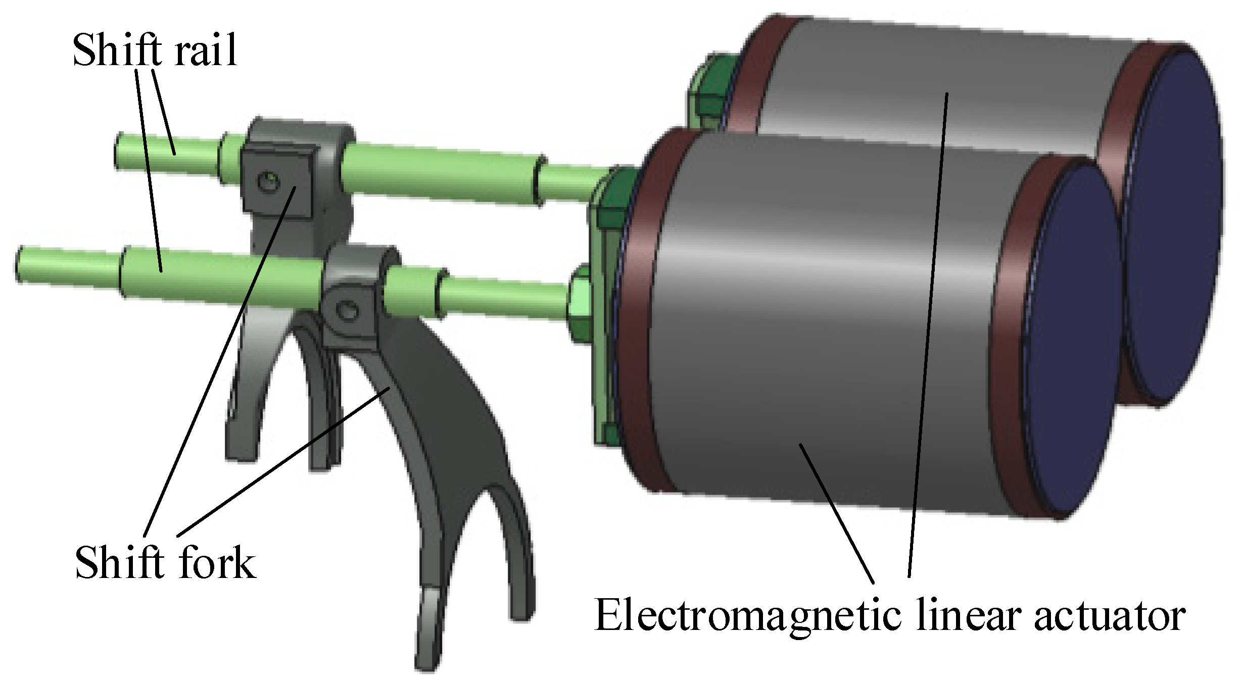Figure 1 shows the novel direct-drive gearshift system. It includes two ELAs, and the output shafts connect with the shift fork directly. Two−way movement of the ELAs will drive the synchronizer through the shift fork to engage a target gear or disengage with the current gear. The intermediate mechanisms such as motion converter and reduction gears which is necessary for a DC motor driven AMT are no longer required. Obviously, the direct−drive gearshift system equipped with ELAs is simpler, and it is beneficial for rapid and precise displacement control. Moreover, Figure 2 presents the inner structure of the ELA prototype.

The test bench of motor−AMT coupled drive system is presented in Figure 3. It consists of ELAs, driving motor, 4−speed AMT, flywheel, torque and speed sensors, adjustable inertia plate and displacement sensors. Each side of the AMT has ELA attached, and 0.01 mm accurate displacement sensors are mounted on the ELAs.

3. Nonlinear Analysis and Modeling of Motor-AMT Coupled Drive System

Nonlinearities exist in numerous complex and integrated systems. However, the nonlinear feature of the motor−AMT coupled drive system has not been studied extensively and comprehensively yet. The output characteristics are frequently nonlinear regardless of the kind of motor−induction motor or permanent magnet synchronous motor. ELAs should be taken into account while modeling the coupled system because they are a source of nonlinearities because of their operating theory and technology limitations. It is also important to study the nonlinearities that will manifest in an AMT’s gearings, shafts, and shift forks when enormous or rapidly fluctuating power is applied. Additionally, because the AMT shifting process is discrete, researchers have divided it into a number of steps in order to develop various control strategies [30]. As a result, the nonlinearities might be produced during the switch of different control strategies and transferring of control parameters.

3.1. Nonlinear Analysis of the ELA

Three subsystems−the electric, magnetic, and mechanical subsystems−can be used to characterize the ELA. Figure 4 displays the mathematical representation of ELA. Transfer lines are another way to show how the three subsystems are coupled. Obviously, the relationship between the input parameter voltage U and output parameter electromagnetic force F_m is nonlinear.

The permanent magnets inside the ELA are arranged using Halbach magnetized topology. Halbach magnetized topology is recognized that it can diminish the saturation of the magnet yoke to enhance the magnetic flux density so that the output electromagnetic force will be enlarged, and it is used to design the ELA. Figure 5a shows the topological structure. The magnetization direction of permanent magnets is represented by the arrowheads. In the space between the permanent magnets, the energized coil moves back and forth. Nevertheless, due to movements, such as those in positions 2 and 3, as shown in Figure 5b, the activated coil would not stay at a constant magnetic field. Hence, the electromagnetic force’s characteristics are variable.

Experiments are performed to examine the output characteristics of ELA. The experiments were implemented as follows,

• Maintain the ELA shaft stationary in the middle and use a force sensor to detect the electromagnetic force as the coil current increases from 0 A to 30 A, increasing by 0.5 A each time;
• Move the ELA shaft forward by 0.5 mm, then uses a force sensor to measure the electromagnetic force while the coil current increases from 0 A to 30 A, with each increment of 0.5 A;
• Using the procedure described above, move the ELA shaft forward by 0.5 mm increments until the displacement reaches 10 mm. Then, measure and record all of the electromagnetic force data;
• Using the procedure described above, move the ELA shaft back to the center position and then backward by 0.5 mm at a time until the displacement reaches 10 mm. Then, record all the electromagnetic force data.

Figure 6 shows the discovered correlations among current, position and electromagnetic force. The static force−displacement−current characteristics are indicated by electromagnetic force and electromagnetic force constant. The ELA has a 20 mm stroke. Obviously, the ELA force characteristics are nonlinear. The electromagnetic force varies with the change of displacement value while the current remains unchanged. The maximum force is produced when the ELA shaft remains in the middle and the displacement value is 10 mm. Additionally, when the current increases, the degree of nonlinearity increases. When the input current I is 10 A, the variation range of the k_m is between 40.1 and 43.4 N/A; when I is 20 A, the k_m is between 39.8 and 42.3 N/A; when I is 30 A, the k_m is between 38.9 and 41.7 N/A. In brief, the nonlinear characteristics of the ELA are influenced by not only the relative displacement of the ELA shaft, but also the variable current. Hence, the nonlinearity of the ELA would affect the precise displacement control during the gearshift process, and proper control method should be designed to eliminate the influence.

3.2. Gearshift Synchronization Process Analysis

Early in 2006, the eight phase equations for the gear engagement procedure of a Borg-Warner synchronizer were explored in reference [30]. The relative position of the spline chamfers and the required turning force were revealed by a thorough investigation of the second-bump and stick−slip phenomena. However, it concentrated on a manual transmission since it has distinct, noticeable characteristics when utilized with an EV’s clutchless motor−AMT coupled drive system. It is necessary to explore the detailed gearshift synchronization process of the motor-AMT coupled drive system. In addition, the gearshift stroke is typically less than 10 mm, making it challenging to develop the proper control strategy for each of the eight distinct stages.

The shifting process is divided into four parts in the author’s earlier work [14], as indicated in Figure 7, and a corresponding control mechanism was developed in accordance with the unique characteristics of each step. For example, the proportion−differentiation approach was developed to accomplish simple, quick, and no-overshot motion control in the first stage, which is to eliminate the gap between the sleeve and the synchronizer ring. However, switching control methods during various stages will result in a hazy transmission of control variables.

For instance, at the end of the first phase, the shift force is not zero, and it would be transmitted to the second phase. Such a transmit of control variables occurs during each of the four phases. Hence, the piecewise control method should be improved to obtain better shift quality. Wang et al. divide the gearshift process into two stages according to the movement state of the sleeve [24]. An integrated position and force switching control scheme including sliding mode control method for nonsynchronous stage and force control for synchronization is developed. Chen et al. use hybrid system theory to analyze the influence of various shifting force, relative rotational position, and speed of synchronization components to shift quality [31]. In fact, the gearshift synchronization process can be viewed as a nonlinear system since the process is discrete while the control variables and the control target are greatly different, and linearization theory should be employed to optimize the control performance.

3.3. Shift Fork Deformation Analysis

The shift fork, which directly transmits the shift force to the synchronizer ring, may deform because the ELA designed for gearshift in this work can output more than 1000 N of electromagnetic force. To assess the influence, it is crucial to measure the shift fork’s deformation values under various shift forces. The finite element model of the shift fork is built with ABAQUS, and two kinds of shift force 500 N and 1000 N are applied on the connection place with ELA shaft.

Figure 8 displays the mesh model and analysis outcomes. With values of 0.26 mm and 0.52 mm, respectively, and shift forces of 500 N and 1000 N, the shift fork’s MAX labeled location experiences the greatest deformation. The distortion is minor when compared to the 9.5 mm space between gearshifts. Compared with the gearshift distance value 9.5 mm, the deformation is nonnegligible. Meanwhile, a larger shift force will result in greater deformation, thus it is best to carry out gearshift events when the rotational speed difference is small, which means that small shift force is transmitted to the shift fork so that the deformation will be negligible. However, it is contradictory to use a greater shift force to achieve a quicker gearshift. As a result, while gear shifting, the shift fork will continue to deform, intensifying the nonlinear properties of the shift force delivered to the synchronizer ring.

3.4. Modeling of the Powertrain System

Shift qualities usually include shift time, shift jerk, friction work and shaft torsional vibration. The shift jerk J is described as follow

$$J=\frac{da\left(t\right)}{dt}=\frac{r}{J_w}\frac{d\left(T_s{i}_d-T_L\right)}{dt}$$

(1)

where a is the accelerate speed of vehicle, r is the radius of wheel, J_w is the equivalent rotational inertia of the vehicle on wheel, T_s is the synchronizing torque, i_d is the gear ratio of main reducing gear, T_L is the load torque.

Apparently, the shift jerk J is mainly influenced by the T_s. Due to the nonlinear characteristics of the shift force, deformation of shift fork and variable control parameters, the value of J will vary fiercely. Moreover, there are two nonlinear components gear pairs and half shaft which the nonlinearities are usually neglected while analyzing the gearshift performance. The nonlinearity of gear pairs happens during the gear mesh process. According to the analysis of literature [27], the nonlinear dynamic characteristics of gear pairs will lower the shift quality, and the torsional vibration of gear pairs will also change the gear ratio. In fact, it is almost impossible to eliminate such influence by using effective method. Nevertheless, with appropriate robust control method, such influence can be weakened. In addition, due to the amplification of the transmission, the transmitted torque on the output shaft of the transmission and half shaft enlarges evidently. As a result, the shafts will show nonlinear vibration feature and it has been verified by He [28]. Such nonlinear vibration feature is more obvious in an EVs since the drive motor has faster torque regulation ability. Hence, the nonlinear feature of shafts should be considered in the simulation model of motor−AMT coupled drive system.

The improved powertrain model of a multi-speed motor−AMT coupled powertrain system is shown in Figure 9. Without the clutch, the powertrain model is simpler without clutch. For the motor, it can be described as

$$J_m{\ddot{\theta }}_m=T_m-T_{\mathrm{in}}-c_m{\dot{\theta }}_m$$

(2)

For the AMT,

$$J_t{\ddot{\theta }}_t=T_{\mathrm{in}}{i}_g-c_t{\dot{\theta }}_t-T_{\mathrm{out}}$$

(3)

where J_m is the rotational inertia of the motor, θ_m is rotational angel, c_m is damping coefficient, T_in is the input torque of AMT, J_t is rotational inertia of AMT, θ_t is rotational angle of the AMT output shaft, c_t is damping coefficient, T_out is output torque of AMT, and θ_m = θ_t i_g.

Meanwhile, the T_out can be described as

$$T_{\mathrm{out}}=k_2\left({\theta }_t-{\theta }_d{i}_d\right)+c_2\left({\dot{\theta }}_t-{\dot{\theta }}_d{i}_d\right)$$

(4)

For the final driver,

$$J_d{\ddot{\theta }}_d=i_d\left[k_2\left({\theta }_t-{\theta }_d{i}_d\right)+c_2\left({\dot{\theta }}_t-{\dot{\theta }}_d{i}_d\right)\right]-c_d{\dot{\theta }}_d-k_4\left({\theta }_d-{\theta }_w\right)-c_4\left({\dot{\theta }}_d-{\dot{\theta }}_w\right)$$

(5)

θ_d is the rotational angle of the final driver, and with θ_d = θ_m/(i_ti_d), the equation can be transformed into

$$J_d{\ddot{\theta }}_m=i_d^2{i}_t\left[k_2\left({\theta }_t-{\theta }_d{i}_d\right)+c_2\left({\dot{\theta }}_t-{\dot{\theta }}_d{i}_d\right)\right]i_d^2{i}_t-c_d{\dot{\theta }}_m-i_t{i}_d\left[k_4\left({\theta }_d-{\theta }_w\right)-c_4\left({\dot{\theta }}_d-{\dot{\theta }}_w\right)\right]$$

(6)

θ_w is the rotational angle of the wheel. For the wheel, the influence of the tire is neglected to simplify the model. Hence, the wheel can be described as

$$\left(J_w+J_v\right){\ddot{\theta }}_w=k_4\left({\theta }_d-{\theta }_w\right)+c_4\left({\dot{\theta }}_d-{\dot{\theta }}_w\right)-T_{\mathrm{load}}=k_4\left(\frac{{\theta }_m}{i_t{i}_d}-{\theta }_w\right)+c_4\left(\frac{{\dot{\theta }}_m}{i_t{i}_d}-{\dot{\theta }}_w\right)-T_{\mathrm{load}}$$

(7)

And the T_load is

$$T_{\mathrm{load}}=\left[M_{\mathrm{vehicle}}g\sin (\alpha \right)+f{M}_{\mathrm{vehicle}}g+\frac{1}{2}{C}_d{A}_F\rho r^2{\dot{\theta }}_v{}^2]$$

(8)

Suppose three state variable x₁, x₂, x₃ are

$$x_1=\frac{{\theta }_m}{i_t{i}_d}-{\theta }_w,x_2={\dot{\theta }}_m,x_3={\dot{\theta }}_w$$

(9)

And the state space equation is obtained,

$$\left[\begin{array}{c}{\dot{x}}_1\\ {\dot{x}}_2\\ {\dot{x}}_3\end{array}\right]=\left[\begin{array}{ccc}0& \frac{1}{i_t{i}_d}& -1\\ \frac{k_d}{J_{eq}{i}_t{i}_d}& \frac{c_4+\frac{c_d}{i_t^2}+\frac{2c_d}{i_t^2{i}_d^2}}{J_{eq}}& \frac{c_4}{i_t{i}_d}\\ \frac{k_4}{J_w}& \frac{c_4}{J_w{i}_t{i}_d}& -\frac{c_4}{J_w}\end{array}\right]\left[\begin{array}{c}{x}_1\\ x_2\\ x_3\end{array}\right]+\left[\begin{array}{ccc}0& 0& 0\\ 0& 1& 0\\ 0& 0& 1\end{array}\right]\left[\begin{array}{c}0\\ T_{\mathrm{m}}\\ T_{\mathrm{load}}\end{array}\right]$$

(10)

where

$$J_{eq}=\frac{J_d}{i_t^2{i}_d^2}+J_m+\frac{J_t}{i_t^2}$$

(11)

The damping coefficient and stiffness coefficient of the shafts are usually considered as constant in the model. However, the study results of references [28] prove that the nonlinearity of stiffness and damping exist in the shafts, and since the half shaft transmits the maximum torque among the shafts, it should consider the nonlinearity of the half shaft while study the dynamic performance of motor−AMT integrated powertrain system. Hence, the parameters k₄ and c₄ should be replaced by functions f_k and f_c [32]. Nonetheless, although it is a compromise way to take the nonlinearity into account, it is hard to implement analyzed results into practical application.

Obviously, several nonlinear influence factors which are neglected commonly exist in the motor−AMT coupled drive system, and according to the above analysis, such factors might cause damage to the gearshift performance. Hence, appropriate control strategy is essential to weaken or even eliminate the effect of nonlinearities.

4. Control Strategy Design

In the author’s previous work, a kind of piecewise control method which contains four different control methods was proposed since the gearshift process can be divided into several phases and each phase has different feature [33]. Nonetheless, the switch of control methods and the transmit of variables among different control methods makes the process disordered and imprecise, and the integration of precise motion control and robust control makes the system complicated.

Afterwards, the piecewise control is replaced with the active disturbance rejection control (ADRC) approach. The basic topology is shown in Figure 10. It includes a tracking differentiator (TD), a nonlinear state error feedback law (NLSEF) and an extended state observer (ESO). It could be thought of as an improved PID approach with disturbance rejection. For the ELA gearshift system, which is influenced by linearities, it is difficult to establish quick and accurate motion control while yet guaranteeing robustness.

Therefore, the ADRC approach needs to be enhanced to meet the control requirements. There are several improvements described as follows. First, the inverse system method (ISM) was used to minimize the nonlinear characteristics of the ELA output force. Second, an acceleration feedforward (AFF) module was introduced to the standard ADRC method to control the displacement of the gearshift process, since it can increase displacement control accuracy [34]. It can partially compensate the disturbance. Furthermore, it is challenging to calculate the compensation value because the shift fork’s deformation varies with the shift force. As a result, the deformation of shift fork is considered as disturbance in this work. Similarly, the nonlinearity of gear pairs will lead to the variation of rotational speed of shafts, and it also can be regarded as external disturbance so that the ESO module can reject such disturbance. In order to enhance the disturbance rejection ability of the controller, the ESO module is modified to improve the rejection ability of the controller.

4.1. Basic Topology of ADRC

The typical form of TD is usually described as

$$\{\begin{array}{l}g=f\left(v_1-v,v_2,r,h\right)\hfill \\ {\dot{v}}_1=v_1+h{v}_2\hfill \\ {\dot{v}}_2=v_2+hg\hfill \end{array}$$

(12)

v₁ is a transitional trajectory, v₂ is the differential of v, and h is the sampling period, g is an intermediate variable. Parameter r influences the dynamic response of v₁, and the larger value of r will shorten the time which is taken by the v₁ of a specific v. The function f(v₁-v, v₂, r, h) is a time−optimal function, which is defined as [34,35]

$$f\left(v_1-v,v_2,r,h\right)=\{\begin{array}{l}d=r·h,d_0=h·d,y=v_1-v+h·v_2\hfill \\ \begin{array}{l}{a}_0=\sqrt{d^2+8r·\left|y\right|}\hfill \\ \begin{array}{l}a=\{\begin{array}{l}{v}_2+\left(a_0-d\right)·\frac{sgn\left(y\right)}{2}, \left|y\right|>d_0\hfill \\ v_2+\frac{y}{h}, \left|y\right|\le d_0\hfill \end{array}\hfill \\ f=\{\begin{array}{l}-rsgn\left(a\right), \left|y\right|>d_0\hfill \\ -\frac{ra}{d}, \left|y\right|\le d_0\hfill \end{array}\hfill \end{array}\hfill \end{array}\hfill \end{array}$$

(13)

Function $fal\left(e,\alpha ,\delta \right)$ is defined as

$$fal\left(e,\alpha ,\delta \right)=\{\begin{array}{l}e\cdot {\delta }^{1-\alpha }, \left|e\right|\le \delta \hfill \\ {\left|e\right|}^{\alpha }\cdot \mathrm{sgn}(e), \left|e\right|>\delta \hfill \end{array}$$

(14)

where α should satisfy α < 1, δ = k_p·h, k_p is a positive integer.

The function of NLSEF is to generate the intermediate input variable u₀. It is described as

$$\{\begin{array}{l}{e}_1=y_1-z_1\hfill \\ e_2=y_2-z_2\hfill \\ u_0={\beta }_{11}\cdot fal\left(e_1,{\alpha }_1,\delta \right)+{\beta }_{12}\cdot fal\left(e_2,{\alpha }_2,\delta \right)\hfill \end{array}$$

(15)

where e₁ and e₂ are estimate errors, z₁ and z₂ are estimated values, β₁₁ and β₁₂ are control parameters, y₁ and y₂ are the output values of the TD module, α₁ and α₂ satisfy the condition 0 < α₁ < 1 < α₂.

ESO module is kernel module of the ADRC since it can estimate the internal and external disturbances according to the analysis of output variables. The discrete time form of the ESO module is

$$\{\begin{array}{l}e=z_1-y\hfill \\ z_1=z_1+h\left(z_2-{\beta }_{01}\cdot e\right)\hfill \\ z_2=z_2+h(z_3-{\beta }_{02}\cdot fal\left(e,\alpha ,\delta \right)+b_0\cdot u\\ z_3=z_3-h\cdot {\beta }_{03}\cdot fal\left(e,\alpha ,\delta \right)\hfill \end{array}$$

(16)

z₁, z₂ and z₃ are estimated values of the output variable y, e is estimate error, h is the sampling time, and any disturbance information is included. β₀₁, β₀₂ and β₀₃ are observer gains and they are usually selected as

$${\beta }_{01\approx 1/h , } {\beta }_{02\approx 1/1.6h^{1.5} , } {\beta }_{03\approx 1/\left(8.6h^{2.2}\right) }$$

(17)

4.2. Design of Inverse System Method

Designing a suitable and reliable control system for a nonlinear system is more challenging than for a linear one. In order to construct a controller for a nonlinear system that will achieve the control aims, the inverse system method is utilized to build a pseudo-linear system for the nonlinear system. A pseudo−linear contains an inverse system and an original system, and the first step is to build the inverse system.

The coupled mathematics shown in Figure 4 allows the mathematical representation of the gearshift system to be rewritten as

$$\{\begin{array}{l}\dot{I}=-\frac{R}{L}I-\frac{k_m}{m}v+\frac{u}{L}\hfill \\ \dot{v}=\frac{k_m}{m}I-\frac{c}{m}v\hfill \\ \dot{S}=v\hfill \end{array}$$

(18)

where I is coil current, R is coil resistance, L is coil inductance, k_m is force constant, v is sleeve’s velocity, m is moving mass, c is viscous friction damping coefficient, S is displacement of the sleeve. The state variables are chosen as

$$\mathit{x}={\left[\begin{array}{ccc}{x}_1& x_2& x_3\end{array}\right]}^T={\left[\begin{array}{ccc}I& v& S\end{array}\right]}^T$$

(19)

Consequently, the state equation is written as

$$\left[\begin{array}{c}{\dot{x}}_1\\ {\dot{x}}_2\\ {\dot{x}}_3\end{array}\right]=\left[\begin{array}{ccc}-\frac{R}{L}& k_m& 0\\ \frac{k_m}{L}& -\frac{c}{m}& 0\\ 0& 1& 0\end{array}\right]\left[\begin{array}{c}{x}_1\\ x_2\\ x_3\end{array}\right]+\left[\begin{array}{c}\frac{1}{L}\\ 0\\ 0\end{array}\right]u, y=\left[\begin{array}{ccc}0& 0& 1\end{array}\right]\left[\begin{array}{c}{x}_1\\ x_2\\ x_3\end{array}\right]$$

(20)

where y is the system output.

According to the inverse system theory, the under equations

$$\{\begin{array}{l}y=x_3\hfill \\ \dot{y}={\dot{x}}_3=x_2\hfill \\ \ddot{y}={\dot{x}}_2=\frac{k_m}{m}I-\frac{c}{m}\dot{y}\hfill \\ \stackrel{⃛}{y}={\ddot{x}}_2=-\frac{c}{m}\ddot{y}+\frac{k_m}{m}\left(-\frac{R}{L}{x}_1-\frac{k_m}{L}\dot{y}+\frac{u}{L}\right)\hfill \end{array}$$

(21)

are obtained. The input variable u specifically only appears in the expression y, hence the inverse system is a third order system with a dimension equal to the state vectors. The system is hence reversible. One solution to the inverse system is

$$u=\frac{ml}{k_m}\stackrel{⃛}{y}+\frac{cl}{k_m}\ddot{y}+k_m\dot{y}+R{x}_1$$

(22)

The chosen state variables for the pseudo linear system are

$$\mathit{w}={\left[\begin{array}{ccc}{w}_1& w_2& w_3\end{array}\right]}^T={\left[\begin{array}{ccc}y& \dot{y}& \ddot{y}\end{array}\right]}^T$$

(23)

and the pseudo−linear system’s state space equations are derived as

$$\{\begin{array}{l}\left[\begin{array}{c}{\dot{w}}_1\\ {\dot{w}}_2\\ {\dot{w}}_3\end{array}\right]=\left[\begin{array}{ccc}0& 1& 0\\ 0& 0& 1\\ 0& 0& 0\end{array}\right]\left[\begin{array}{c}{w}_1\\ w_2\\ w_3\end{array}\right]+\left[\begin{array}{c}0\\ 0\\ 1\end{array}\right]\phi =\mathit{A}\mathit{w}+\mathit{B}\phi \hfill \\ y=\left[\begin{array}{ccc}1& 0& 0\end{array}\right]\left[\begin{array}{c}{w}_1\\ w_2\\ w_3\end{array}\right]=\mathit{C}\mathit{w}\hfill \end{array}$$

(24)

State feedback controllers are made to characterize the dynamic properties of control input and output for pseudo−linear systems. The target equation is created as

$$y^k\left(t\right)+a_{k-1}{y}^k\left(t\right)+\dots +a_1{y}^{\prime }\left(t\right)+a_{0}y\left(t\right)=r\left(t\right)$$

(25)

where $a_0$, $a_1$, …, $a_{k-1}$ are real number, and $r\left(t\right)$ is reference input.

The following control law can be established using state feedback control theory because the pseudo linear system’s state variables are three

$$\{\begin{array}{l}\phi =r-y_f\hfill \\ y_f=a_{0}y+a_1\dot{y}+a_2\ddot{y}\hfill \end{array}$$

(26)

where $r$ is the desired value and $y_f$ is the feedback value. The transfer function can be deduced as

$$\frac{Y\left(s\right)}{R\left(s\right)}=\frac{1}{s^3+a_2{s}^2+a_{1}s+a_0}$$

(27)

Consequently, the transfer function’s characteristic equation is

$$\left(s^2+2\varsigma {\omega }_n+{\omega }_n^2\right)\left(s+\varsigma {\omega }_n\right)=0$$

(28)

where $\varsigma$ is the damping coefficient, ${\omega }_n$ is the natural frequency. The transition time can be calculated by equation $t_s\approx 4/\varsigma {\omega }_n$, and the standard damping coefficient is chosen to be 0.707. The natural frequency is 282.88 since the transition period is calculated to be 20 ms. Put $\varsigma$ and ${\omega }_n$ into the characteristic Equation (28), the following equation are obtained

$$s^3+600s^2+160021.1s+16004218.9=0$$

(29)

By applying Ackermann formula, a₂ = 600, a₁ = 160021.1, a₀ = 16004218.9 is obtained.

4.3. Improvement of ESO Module

The observation and estimation performance of the ESO is mainly decided by the nonlinear function fal(e, α, δ). Function fal(e, α, δ) is widely used due to its simple structure. However, the continuity and flatness of the fal function has potential to be improved especially near the original point [36]. A higher error feedback gain will improve the ESO module’s ability to observe and convergence rate, but it will also amplify signal noise and other disturbances that threaten the stability of the control system [37]. As a result, a kind of novel nonlinear function faln(x, σ)vis employed to solve the problem. The faln(x, σ) is designed as

$$faln\left(x,\sigma \right)=\{\begin{array}{c}\frac{x}{{\sigma }^2}{e}^{-\frac{x^2}{2{\sigma }^2}},\left|x\right|\ll 1\\ \frac{1}{{\sigma }^2}{e}^{-\frac{1}{2{\sigma }^2}},x>1\\ -\frac{1}{{\sigma }^2}{e}^{-\frac{1}{2{\sigma }^2}},x<-1\end{array}$$

(30)

where σ is the regulation parameter. According to the analysis in literature [34], the faln function, which only has one parameter as opposed to the fal function’s two, is superior to the fal function in terms of observation and noise rejection. Obviously, the control system design is simplified and the performance of ESO is enhanced. The designed controller is presented in Figure 11.

4.4. Comparative Simulation and Analysis

Comparative simulations were carried out to verify the performance of the designed method. First, displacement control performance of the ADRC method is simulated and meanwhile PID method is employed as a comparison group to realize the same displacement control. Figure 12 shows the comparative results. There are three different target displacement values chosen: 2 mm, 4 mm and 9.5 mm. When the displacement value is 4 mm, the control parameters of the two controllers are regulated and established, and they remain constant when the displacement value changes. It can be discovered that both controllers can reach the target displacement value quickly, however the ADRC controller is noticeable quicker than the PID controller. Furthermore, when the target value is 9.5 mm, the displacement of the PID technique is greater than the target value. Obviously, the ADRC controller has superior parameter-dependent stability than the PID controller. On the other hand, every displacement curve reaches the desired value in less than 25 ms, demonstrating the actuator’s quick dynamic performance.

Figure 13 displays the disturbance rejection ability of three different types of controllers, including IADRC, ADRC and PID controllers. An external load torque is injected at 11 ms to observe the performance of the three controllers. PID controller presents the most distinct variation among the three controllers, and stead−state error of the displacement control is also produced. Only a little change in the displacement curve is observed when using the ADRC and IADRC controllers, which appear to have higher disturbance rejection capabilities. Additionally, IADRC controller has quicker adjusting ability than ADRC controller. Obviously, the AFF module enhances the IADRC controller’s quick dynamic performance, and the modified ESO strengthens its capacity to reject disturbances.

Figure 14 shows the displacement tracking performance. The target displacement curve is designed and divided into four stages as the real displacement variation of the gearshift process. Obviously, the IADRC tracks the target curve best both on the time and precision indexes. In brief, the IADRC controller presents faster dynamic performance, more accurate displacement control and better stability to the parameter variations and external disturbances.

5. Experiments and Analysis

Figure 3 displays the test bench in detail. The motor-transmission coupled drive system and the direct drive gearshift system that are proposed in this work are primarily for EVs. Since the drive motor is often under active speed regulation control, the speed difference is less than with regular AMT. As a result, two types of speed differences−100 and 300 r/min−are chosen to verify the gearshift performance of the direct drive gearshift system. As it is known, shift time, jerk, and friction work make up the majority of the gearshift performance indices. Due to the rapid development of the material and manufacturing technique, the service life of the synchronizer ring is distinctly extended. Meanwhile, the friction work apparently decreases since the speed difference is smaller in EVs. Friction work is therefore not the primary focus of this work. In earlier research, the performance of the ADRC approach was found to be superior to the PID method overall in terms of both the accuracy of displacement control and the capacity to reject disturbances. Therefore, in this work, the IADRC method and the ADRC approach are compared.

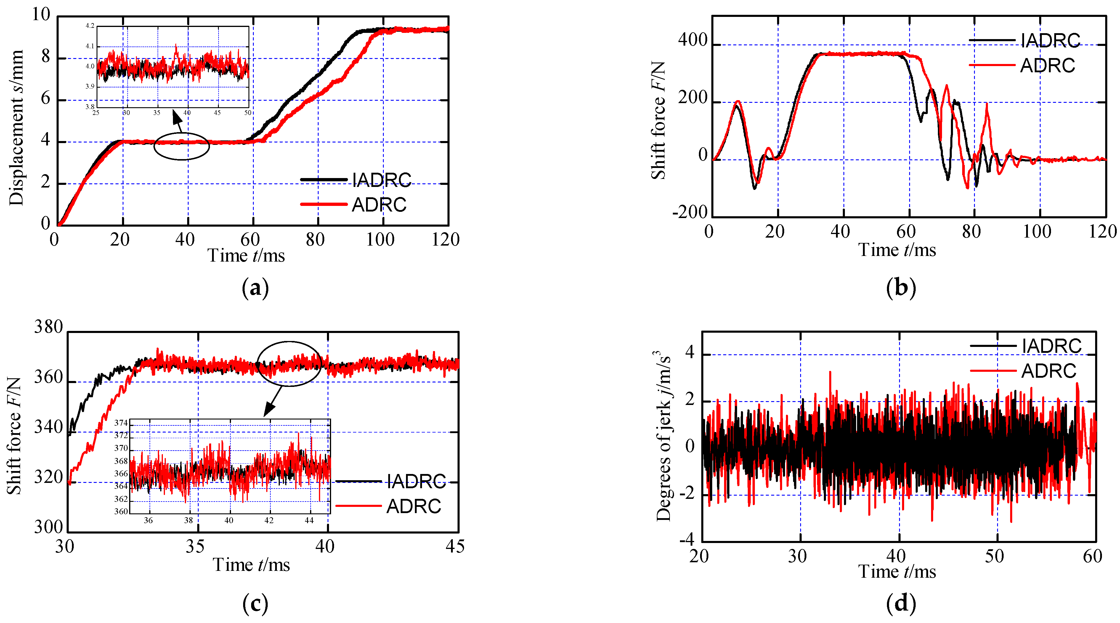
Figure 15 shows the gearshift displacement, shift force and jerk of the gearshift process when the speed difference is 100 r/min. It can be seen from the Figure 15a shows that the gearshift time for the two control methods is less than 100 ms, and the values are 93.4 ms and 100.1 ms respectively. One of the important reasons is that the IADRC approach performs dynamically more quickly, which reduces a few shift times during stage (a)(c)(d) that include displacement increments.

Additionally, the partial enlarged drawing in Figure 15a illustrates the fluctuation of the displacement during the synchronization process. The fluctuation is mainly produced by the nonlinear of shift force, deformation of shift fork, accuracy error of displacement sensor and external disturbances including vibration, and it will influence the friction torque loaded on the synchronizer mechanisms so as to slow the synchronization process. All these disturbance factors lead to the fluctuation of the displacement. Apparently, the displacement fluctuation of the IADRC method is smaller than that of the ADRC method. Although the disturbance rejection ability of the ADRC method is excellent [34,35,36], the improved IADRC method can suppress the disturbances better.

In addition, the four stages described in Figure 7 are not very clear on the displacement curve of IADRC method in Figure 15a. The reason is that the teeth of the sleeve pass by the teeth of the target gear without distinct contact so that the displacement increases smoothly. On the contrary, there is a tiny standstill of the displacement on the curve of ADRC. It usually costs several seconds for the sleeve to revolve at just the right angle so as to cross the teeth of the target gear.

The shift force suggests that the two controllers are performing similarly. The amplified drawing of the synchronization process is presented in Figure 15c. Since the speed difference is comparatively small, the shift time will be small too. To achieve the proper shift jerk, the maximum shift force is therefore restricted to a certain value. The maximum shift force usually happens in the synchronization process. It is clear that both of the two curves in Figure 15c exhibit variance. However, the fluctuation amplitude of the of the shift force is smaller when the IADRC technique is adopted which let the ELA output force have better linear properties. For the ADRC approach, the fluctuation range is 362 to 373 N, whereas for the IADRC method, it is 363 to 370 N. Also, it is beneficial to decrease shift time. The shift force curve clearly shows the four steps. The second stage ends when the shift force starts to rapidly fall after the first stage, which takes over 20 ms. In the third stage, it usually needs a bump force to turn the sleeve so as to cross the teeth of the target gear. After that, the teeth of the sleeve will come into contact with those of the target gear, necessitating another bump force to cause the sleeve to turn at a slight angle once more in order to mesh with the gear. Therefore, there are two bump force existing on the shift force curve.

The degree of jerk is shown in Figure 15d. Due to the limitation of maximum shift force, the degrees of jerk are all acceptable for both methods. For the IADRC method and the ADRC method, the maximum degrees of jerk are 2.31 m/s³ and 3.13 m/s³, respectively. The shift jerk is directly caused by the drastic contact of two components, however, the deformation of shift fork, fluctuation of displacement, control parameter variations and external vibrations will also result in unpredictable shift jerk. The improve ESO module of IADRC method can estimate such factors from the output variables, and proper adjustment will produce to limit the influence of those disturbances to the shift fork. Moreover, the linearization of the ELA output force is also helpful to reduce the shift jerk. Apparently, it appears that the IADRC can restrain the jerk to a better degree than ADRC approach, and it demonstrate the better disturbance rejection ability and the effectiveness of the IADRC method.

Figure 16 depicts the gearshift displacement, shift force and jerk of the gearshift process when the speed difference is 300 r/min. The limitation of shift force increases to 600 N to guarantee small shift time and degree of jerk. For the IADRC method and the ADRC approach, the shift times are 121 ms and 137 ms, respectively. Both curves exhibit displacement fluctuation, however it is less evident when the IADRC approach is used. The displacement value during the synchronization process is nearly 4.1 mm while it is nearly 4 mm when the speed difference is 100 r/min. It is caused by the increase of the shift force during the synchronization process. Larger force will produce slight deformation of the shift fork, and the deformation will transfer to the displacement sensor. In addition, the amplitude of fluctuation of the shift force becomes bigger since the nonlinear output characteristics will be more obvious with the increase of shift force. Similarly, the IADRC method has better performance than ADRC method in terms of restraining the nonlinear output characteristics of the ELA. Although the degrees of jerk appear slight increase with the values presented in Figure 15, they are still acceptable since all the values are smaller than 4 m/s³. The specific values of shift time, synchronization time and degrees of jerk are all given in

Table 1. Gearshift indexes of 30 times gearshift events.

Speed Difference (r/min)	Inertia (kgm2)	Control Method	Gearshift Time (ms)	Synchronization Time (ms)	Maximum Jerk(m/s3)
100	0.03	IADRC	90~94	39~42	2.31
	0.03	ADRC	95~101	44~48	3.13
	0.05	IADRC	121~130	65~71	2.70
	0.05	ADRC	127~143	66~75	3.48
300	0.03	IADRC	120~127	68~73	2.57
	0.03	ADRC	128~145	74~82	3.91
	0.05	IADRC	165~180	111~119	2.79
	0.05	ADRC	169~188	112~126	3.96

.

Another inertia value 0.05 kgm² is chosen to perform gearshift events in order to further confirm the effectiveness and advantages of the designed method, and the outcomes of 30 times of gearshift events are presented in Table 1. When the speed differential or inertia value grows, the gearshift time also grows. Similar change rules are presented by the maximum jerk and synchronization time. Meanwhile, the maximum values of friction work per unit during these gearshift events is 0.13 J/mm², which is smaller than the permission value 1.2 J/mm² evidently. It can be concluded that the IADRC method has better comprehensive control performance than ADRC method. The ISM technique can linearize the output force characteristics of the ELA so that both the shift jerk and fluctuation of displacement is smaller, and the optimized ESO module improve the disturbance rejection ability compared with that of the ADRC method. In short, the IADRC method can achieve better gearshift performance than ADRC method from Table 1, and the effectiveness of the IADRC method is also proved by experiments.

6. Conclusions

This paper introduced a type of direct−drive gearshift system that used two electromagnetic linear actuators (ELAs). The direct-drive gearshift system, which gains from the ELAs’ powerful drive capabilities and the system’s direct-drive design, has the potential to enhance shifting performance, including gearshift time and jerk. The gearshift system’s nonlinear properties were taken into account and examined in order to build the best control strategies to lessen the impact of the nonlinearities.

A kind of improved active disturbance rejection control (IADRC) method was designed. It is derived from the ADRC method, and it has the advantages of a simple structure and strong robustness. The ELA’s nonlinear output characteristics are lessened when the inverse system method (ISM) is used, and the IADRC method’s ability to reject disturbances is improved by optimizing the ESO module. In addition, the use of an acceleration feedforward module improved the dynamic response of the controller.

Comparative simulations and experiments were conducted, and the findings indicated the effectiveness and improvement of the designed IADRC method. In conclusion, the IADRC method has better gearshift performance than the ADRC method. Moreover, with the application of the IADRC method, the direct-drive gearshift system employing two ELAs has excellent gearshift performance. Further studies will focus on the coordinated control of the motor−transmission coupled drive system to achieve a fast, comfortable and seamless EV drive system.