Multi-Agent Reinforcement Learning with Optimal Equivalent Action of Neighborhood

Abstract

In a multi-agent system, the complex interaction among agents is one of the difficulties in making the optimal decision. This paper proposes a new action value function and a learning mechanism based on the optimal equivalent action of the neighborhood (OEAN) of a multi-agent system, in order to obtain the optimal decision from the agents. In the new Q-value function, the OEAN is used to depict the equivalent interaction between the current agent and the others. To deal with the non-stationary environment when agents act, the OEAN of the current agent is inferred simultaneously by the maximum a posteriori based on the hidden Markov random field model. The convergence property of the proposed methodology proved that the Q-value function can approach the global Nash equilibrium value using the iteration mechanism. The effectiveness of the method is verified by the case study of the top-coal caving. The experiment results show that the OEAN can reduce the complexity of the agents’ interaction description, meanwhile, the top-coal caving performance can be improved significantly.

1. Introduction

Optimal decision-making in a multi-agent system with uncertainty [1,2,3] in the non-stationary environment [4,5,6] is a challenging problem. Reinforcement learning (RL) [7,8] is an effective method to yield the optimal decision of the multi-agent system based on the Markov decision-making process and dynamic programming [9,10,11,12,13,14]. Theoretically, each agent calculates its action based on the current state and the interaction with other agents. The calculation always retraces all the possible decision processes from the terminal state, and the complexity will become exponential with a higher number of agents [15]. The method to obtain the cooperative policy of each agent is based on the Q-value about state and joint actions of a multi-agent system [16,17]. Hence, how to establish the expression of Q-value to describe the interaction structure among the agents is one of the most important issues in a multi-agent system.

The existing approaches include recording all interactions among agents [15,18,19]. In these methods, each agent has its Q-value function to depict the joint actions of all the other agents. Hence, it can fully present the relationships of any agent pair. However, the computing complexity will rise dramatically as well as the space complexity. More importantly, it is even impossible to enumerate all the relationships if the number of agents is very large. Employ graph network is a new method to establish the relationship among the agent [20], establishes a graph network to describe attention. The target agents and traffic participants are covered by the graph network [21] proposes a graph-based attention communication method to coordinate the interactions of scheduler and message processor.

Sharing neighbors’ equivalent actions is another effective method to construct the interaction among agents. The parameters of the Q-value function include the action value of the current agent and the equivalent action of the agents in the neighbours. That reduces the number of Q-value functions and decreases the learning complexity significantly. These approaches [18,22] obtain the optimal decision of two competitor agents, in which the opponent action of the current agent could be considered to be a special kind of equivalent action. A computation rule to calculate joint action for Q-value function is proposed to reduce the compute complexity [23], and the Q-value function of the current agent is designed using the neighborhood equivalent action [24]. They do not consider the incidence relation of all the agents, hence the memory space for training the Q-value is smaller and the training process is faster.

In a multi-agent system, if the neighborhood agents choose optimal action, the current agent could obtain the optimal action more easily. Based on this, we develop a new Q-value function to depict the environment state, the current agent action, and the optimal equivalent action of the neighborhood agents.

However, it is well-known that the environment of a multi-agent system is non-stationary when the agents execute their policy [25,26]. Therefore, it is hard to obtain the optimal equivalent action from the neighbors. To address these issues, this paper proposes a multi-agent optimal decision method based on a new Q-value function that consists of the system state, the current agent action, and the optimal equivalent action of the neighborhood (OEAN). To obtain the OEAN, the hidden Markov random field (HMRF) is employed to establish the probability graphical model (PGM) [22] for the multi-agent system decision, then the OEAN is obtained by the maximum a posterior (MAP) estimation. The main contribution of this work includes:

(1) A new Q-value function based on OEAN is proposed to establish the interaction between the current agent and its neighbors, so that the current agent could obtain the optimal decision more easily.

(2) The PGM is used to infer the optimal actions of agents in the neighborhood by the MAP, based on the HMRF model, to avoid the issue due to non-stationary environment. The OEAN of the current agent is calculated based on the PGM inference result.

(3) The learning mechanism of the new Q-value function based on the OEAN is presented to guarantee the Q-value converging to the global Nash equilibrium.

The remainder of the paper is organized as follows. Section 2 presents related work in order to motivate our work. In Section 3, the new Q-value function is proposed for the multi-agent RL. In Section 4, the HMRF model is employed to estimate the OEAN, and the convergence of the method is proved. In Section 5, the experiment of top-coal caving demonstrates the effectiveness of the method. The conclusion is given in Section 6.

2. Related Work

This paper addresses the issue of multi-agents optimal decision by RL with PGM. Setting the independent Q-value function for each agent is the direct method [25,27], in which the interaction of each agent is depicted by the actions of the current agent and the other agents [28]. In 2003 [29], proposed the Nash Q-learning to the non-cooperative multi-agent, and the RL iteration can converge to the Nash equilibrium point. A similar convergence proof can be found in [30,31]. At present, Nash Q-learning is extended to electricity markets [32], interconnected multi-carrier systems [33], continuous control systems [34], etc. However, if the agent number is huge, the calculation and storage for depicting the relationship between each current is complex. To decrease the calculation and storage [24], defines a new Q-function, in which the neighbor’s action is transformed into an equivalent action based on mean field theory. In this paper, we propose a new Q-value function based on the optimal OEAN along the way of above references.

The OEAN is inferred by PGM. Actually, PGM is one of the effective ways to describe the Markov decision problem by RL, in which the random field is used to formulate the relationship of agents by node and edge [35]. The implementation of PGM for Markov decision process often includes the Bayesian network [36,37,38] and the conditional random field [39,40] and they are classical model-based method, which means the ground truth is often needed to train the parameters of the model.

Nevertheless, the environment of the multi-agent system is non-stationary during the decision process [41], hence it is difficult or even impossible to obtain the ground truth. The Hidden Markov Model (HMM) [42] is an available method to deal with parameter learning without ground truth in RL, in which the unknown ground truth is action considered to be a hidden variable [43]. At present, to the best of our knowledge, HMM is employed to deal with the signal-agent systems due to the principle of HMM is restricted for a single Markov decision. Hidden Markov random field (HMRF) [44] extends the single hidden variable to a hidden random field. Despite the fact that it is proposed to deal with image segmentation problem [44,45], it provides an available method to infer the optimal decision without ground truth.

This paper follows Nash Q-learning and proposes a new Q-value function based on OEAN for the optimal decision of multi-agent based on HMM and HMRF.

3. Reinforcement Learning Based on the OEAN

3.1. Background

For the decision process of a multi-agent system, let the state space be $\mathcal{S}$, and the state of the multi-agent system be $s\in \mathcal{S}$, the action space be $\mathcal{A}$. For agent i, let its action be $a_i\in {\mathcal{A}}_i$, where ${\mathcal{A}}_i\subseteq \mathcal{A}$. The Markov decision process of the agents is defined as $\mathcal{M}\triangleq \{\mathcal{S};{\mathcal{A}}_1,\dots ,{\mathcal{A}}_N;r_1,\dots ,r_N;p;\gamma \}$, where N is the agents number, the discount factor of reward is $\gamma$, $\gamma \in (0,1)$. For agent i:

(1) the reward function is $r_i:\mathcal{S}\times {\mathcal{A}}_1\times \dots \times {\mathcal{A}}_N\to \mathbb{R}$;

(2) the transition probability is $p:\mathcal{S}\times {\mathcal{A}}_1\times \dots \times {\mathcal{A}}_N\to \mathsf{\Gamma }\left(\mathcal{S}\right)$, $\mathsf{\Gamma }\left(\mathcal{S}\right)$ describes the states’ transition probability distribution over $\mathcal{S}$;

(3) the policy is defined as ${\pi }_i(a_i\mid s):\mathcal{S}\to {\mathsf{\Gamma }}_A\left({\mathcal{A}}_i\right)$, ${\mathsf{\Gamma }}_A\left({\mathcal{A}}_i\right)$ characterizing the probability distribution over action space ${\mathcal{A}}_i$; the joint policy of all the agents is $\pi$, $\pi =[{\pi }_1,\dots ,{\pi }_N]$.

If the multi-agent system initial state is s, the value function of agent i under the joint policy $\pi$ is formulized as

$$\begin{array}{c}\hfill v_i^{\pi }\left(s\right)={\mathbb{E}}_{\pi }\left(\sum _{t=0}^{\infty }{\gamma }^t{r}_i^t\mid s\right)\end{array}$$

(1)

The action value function of agent i under the joint policy $\pi$ is defined as $Q_i^{\pi }:\mathcal{S}\times {\mathcal{A}}_1\times \dots \times {\mathcal{A}}_N\to \mathbb{R}$, and

$$\begin{array}{c}\hfill Q_i^{\pi }\left(s,a\right)=r_i\left(s,a\right)+\gamma {\mathbb{E}}_{s^{\prime }\sim p}\left(v_i^{\pi }\left(s^{\prime }\right)\right)\end{array}$$

(2)

where $a=\left[a_1,\dots ,a_N\right]$ is the action of each agent under the joint policy $\pi$, $s^{\prime }$ is the state of next step. By Equation (1), the action value function can be rewritten as

$$\begin{array}{c}\hfill v_i^{\pi }\left(s\right)={\mathbb{E}}_{\pi }\left(Q_i^{\pi }\left(s,a\right)\right)\end{array}$$

(3)

In the multi-agent system, the input and output of the agents could be, respectively, considered to be a random field of states and a Markov random field (MRF) of the actions. In this paper, we suppose the input random field is the state of the multi-agent s, and the MRF of action is denoted by $a=\left\{a_1,\dots ,a_N\right\}$. In the multi-agent system, each action value function $Q\left(s,a\right)$ with the joint action of its neighborhood could be factored as follows [24].

$$\begin{array}{c}\hfill Q_i\left(s,a\right)=\frac{1}{\lfloor N_i\rfloor }\sum _{k\in N_i}{Q}_i\left(s,a_i,a_k\right)\end{array}$$

(4)

where $N_i$ is the neighborhood of agent i, and $\lfloor N_i\rfloor$ is the neighborhood size.

For agent i, the Q-value function with joint actions can be estimated by an approximated function $Q_i\left(s,a_i,{\overline{a}}_i\right)$, ${\overline{a}}_i$ is the equivalent action of the neighborhood. This conclusion can be found in [24] shown as the following lemma.

Lemma 1

([24]). In a multi-agent system, for agent i, the neighborhood is $N_i$, in which the agent k belongs to $N_i$, $k\in N_i$; ${\overline{a}}_i$ is the equivalent action of $N_i$, ${\overline{a}}_i=\frac{1}{\lfloor N_i\rfloor }{\sum }_{k\in N_i}{a}_k$, such that $Q_i\left(s,a\right)$ can be expanded into Taylor series at the point $\left(s,a_i,{\overline{a}}_i\right)$, and $Q_i\left(s,a\right)$ can be approximated as $Q_i\left(s,a_i,{\overline{a}}_i\right)$, i.e.,

$$\begin{array}{c}\hfill Q_i\left(s,a\right)\approx Q_i\left(s,a_i,{\overline{a}}_i\right)\end{array}$$

(5)

3.2. Multi-Agent Policy with the OEAN

When the current agent makes a decision in a multi-agent system, if the actions of neighborhood agent $N_i$ are optimal, the current agent i could be easily to obtain the optimal action. Hence, we define the optimal equivalent action of the neighborhood (OEAN) as follows to describe the neighborhood condition:

$$\begin{array}{c}\hfill {\overline{a}}_i^{*}=\frac{1}{\lfloor N_i\rfloor }\sum _{k\in N_i}{a}_k^{*}\end{array}$$

(6)

where $a_k^{*}$ is the optimal action of agent k in the neighborhood $N_i$. Based on the OEAN, this paper proposes a new action value function $Q_i\left(s,a_i,{\overline{a}}_i^{*}\right)$ to describe the relation of the environment, the current agent, and the equivalence of the neighbors.

It should be noted that ${\overline{a}}_i^{*}$ is result of picking the optimal equivalent action in the optimal action $a_k^{*}$ of neighborhood, $k\in N_i$. We denote the equivalent policy of neighborhood agents as ${\overline{\pi }}_i$. That means if all the neighborhood agents obtain the optimal policy, ${\overline{\pi }}_i$ is an optimal equivalent policy, and the policy decided by Q-value function for the current agent would be more directly and feasibly. ${\overline{\pi }}_i$ is a hypothesis policy because it is difficult to directly calculate the optimal action of the neighbors on time in the non-stationary environment, and the estimating method of OEAN ${\overline{a}}_i^{*}$ will be given in Section 4.

According to Lemma 1 and Q-learning algorithm [7], we consider the OEAN ${\overline{a}}_i^{*}$ to substitute the equivalent action ${\overline{a}}_i$, and establish the learning mechanism for the Q-value function as follows:

$$\begin{array}{cc}\hfill & Q_i^{t+1}\left(s,a_i,{\overline{a}}_i^{*}\right)=\left(1-\alpha \right)Q_i^t\left(s,a_i,{\overline{a}}_i^{*}\right)+\alpha \left(r_i+\gamma v_i^t\left(s^{\prime }\right)\right)\hfill \end{array}$$

(7)

where

$$\begin{array}{cc}\hfill v_i^t\left(s^{\prime }\right)& ={\mathbb{E}}_{{\overline{\pi }}_i\left({\overline{a}}_i^{*}\mid s^{\prime }\right)}{\mathbb{E}}_{{\pi }_i^t\left(a_i\mid s^{\prime },{\overline{a}}_i^{*}\right)}{Q}_i^t\left(s^{\prime },a_i,{\overline{a}}_i^{*}\right)\hfill \end{array}$$

(8)

in which $\gamma \in \left[0,1\right)$ is the discount factor, $\alpha$ is the learning rate; $\pi$ shown as follows is the policy of the agent i.

$$\begin{array}{c}\hfill {\pi }_i^t\left(a_i\mid s,{\overline{a}}_i^{*}\right)=\frac{exp\left(\beta Q_i^t\left(s,a_i,{\overline{a}}_i^{*}\right)\right)}{{\sum }_{a_i^{\prime }\in {\mathcal{A}}_i}exp\left(\beta Q_i^t\left(s,a_i^{\prime },{\overline{a}}_i^{*}\right)\right)}\end{array}$$

(9)

As we all know, training the Q-value function converging to optimal value is one of the keys in RL. In the dynamic environment, the system state depends on the executing action. Hence the Q-value function is difficult to train due to the fact that the state space is hard to be covered especially when the system is huge. This paper proposes a state extension training method for an especially kind RL in which the state and the corresponding reward meets the following condition:

$$\begin{array}{c}\hfill r\left(a_k\mid s_j\right)\ge r\left(a_k\mid s_{j-1}\right)\end{array}$$

(10)

where $a_k\in \mathcal{A}$, $s_j,s_{j-1}\in \mathcal{S}$, $s_j$ is the next state of $s_{j-1}$. Equation (10)) means the reward function is a monotonous regarding to the same action. If the current state is $s_j$, the following state extension training method can accelerate the Q-value function training.

$$\begin{array}{c}\hfill \left\{\begin{array}{cc}{\displaystyle \coprod _{k=j+1,j+2,\dots ,L}}M\left(k\right),\hfill & \hfill if{r}_i>0\\ \\ {\displaystyle \coprod _{k=1,2,\dots ,j}}M\left(k\right),\hfill & \hfill if{r}_i\le 0\end{array}\right.\end{array}$$

(11)

where $M\left(k\right)$ is the learning mechanism

$$\begin{array}{c}\hfill Q_i^{t+1}\left(s_j,a_i,{\overline{a}}_i^{*}\right)=\left(1-\alpha \right)Q_i^t\left(s_j,a_i,{\overline{a}}_i^{*}\right)+\alpha \left(r_i+\gamma {\mathbb{E}}_{{\overline{\pi }}_i}{\mathbb{E}}_{{\pi }_i^t}{Q}_i^t\left(s^{\prime },a_i,{\overline{a}}_i^{*}\right)\right)\end{array}$$

(12)

and $\coprod _{k}M\left(k\right)$ means $M\left(k\right)$ execute the learning process.

3.3. Nash Equilibrium Policy Based on the OEAN

In the multi-agent system, the agents learn action value function $Q^t$ converging to the optimal policy. In the learning process, the policy is denoted by ${\pi }^t=\left[{\pi }_1^t,\dots ,{\pi }_N^t\right]$. If the agent obtains its optimal policy non-cooperatively, the multi-agent system could achieve Nash equilibrium [46].

The Nash equilibrium policy of the multi-agent system is denoted by ${\pi }^{*}$. Actually, the policy is produced by Q, hence the Nash equilibrium of Q-value function $Q^{*}$ is equivalent to the ${\pi }^{*}$.

For agent i, generally, the global Nash equilibrium policy is defined as follows:

$$\begin{array}{c}\hfill {\mathbb{E}}_{{\pi }_{-i}^{*}}{\mathbb{E}}_{{\pi }_i^{*}}{Q}_i\left(s,a_i\right)\ge {\mathbb{E}}_{{\pi }_{-i}}{\mathbb{E}}_{{\pi }_i}{Q}_i\left(s,a_i\right)\end{array}$$

(13)

and the Nash equilibrium saddle of the policy is defined as Equation (14)

$$\begin{array}{cc}\hfill & {\mathbb{E}}_{{\pi }_{-i}^{*}}{\mathbb{E}}_{{\pi }_i^{*}}{Q}_i\left(s,a_i\right)\ge {\mathbb{E}}_{{\pi }_{-i}^{*}}{\mathbb{E}}_{{\pi }_i}{Q}_i\left(s,a_i\right)\hfill \\ \hfill & {\mathbb{E}}_{{\pi }_{-i}^{*}}{\mathbb{E}}_{{\pi }_i^{*}}{Q}_i\left(s,a_i\right)\le {\mathbb{E}}_{{\pi }_{-i}}{\mathbb{E}}_{{\pi }_i^{*}}{Q}_i\left(s,a_i\right)\hfill \end{array}$$

(14)

where ${\pi }_{-i}=\left[{\pi }_1,\dots ,{\pi }_{i-1},{\pi }_{i+1},{\pi }_N\right]$.

The OEAN of the current agent means the neighbourhood agents obtain the optimal policy; hence, we defined the Nash equilibrium policy based on the OEAN as follows:

$$\begin{array}{c}\hfill {\mathbb{E}}_{{\overline{\pi }}_i}{\mathbb{E}}_{{\pi }_i^{*}}{Q}_i\left(s,a_i,{\overline{a}}_i^{*}\right)\ge {\mathbb{E}}_{{\overline{\pi }}_i}{\mathbb{E}}_{{\pi }_i}{Q}_i\left(s,a_i,{\overline{a}}_i^{*}\right)\end{array}$$

(15)

We should note that ${\overline{\pi }}_i$ is an equivalent policy of the agents in neighbourhood, and the neighbor agents are supposed to obtain the optimal policy. Because ${\overline{\pi }}_i$ is an optimal equivalent policy, hence based on OEAN, the agent just has the global Nash equilibrium policy.

The proposed learning mechanism of $Q_i\left(s,a_i,{\overline{a}}_i^{*}\right)$ is shown in Equation (8). It can converge to the Nash equilibrium defined above. The convergence proof will be given in the next section.

4. OEAN Based on HMRF

4.1. HMRF for Multi-Agent System

According to the defined random field and MRF for multi-agent system in Section 3.1, the input states of the system $s=\left\{s_1,\dots ,s_N\right\}$ can be considered to be the observable random variables, and the output $a=\left\{a_1,..,a_N\right\}$ can be regarded as the latent random variables. Hence, we employ the hidden Markov random field (HMRF) [47] to estimate the optimal action of agent in the neighbourhood.

Suppose that the conditional probability distribution of each state $p\left(s_i\mid a_i\right)$ follows the same function $f\left(s;{\theta }_{a_i}\right)$, i.e.,

$$\begin{array}{c}\hfill p\left(s_i\mid a_i\right)=f\left(s;{\theta }_{a_i}\right)\end{array}$$

(16)

This paper assumes that each element in the random fields of the state and the corresponding action is conditional independent, therefore we can obtain the following result:

$$\begin{array}{c}\hfill p\left(s\mid a\right)=\prod _{i}p\left(s_i\mid a_i\right)\end{array}$$

(17)

Define the neighborhood set of agent i is $N_i$, $i\notin N_i$ and the following result can be yielded [44]

$$\begin{array}{cc}\hfill p\left(s_i,a_i\mid N_i\right)& =p\left(s_i\mid a_i,N_i\right)p\left(a_i\mid N_i\right)\hfill \\ \hfill & =p\left(s_i\mid a_i\right)p\left(a_i\mid N_i\right)\hfill \end{array}$$

(18)

The marginal probability distribution of $s_i$ under the condition of $N_i$ is

$$\begin{array}{cc}\hfill p\left(s_i\mid N_i;{\theta }_{a_i}\right)& =\sum _{a_i\in {\mathcal{A}}_i}p\left(s_i,a_i\mid N_i\right)\hfill \\ \hfill & =\sum _{a_i\in {\mathcal{A}}_i}f\left(s;{\theta }_{a_i}\right)p\left(a_i\mid N_i\right)\hfill \end{array}$$

(19)

where the prior probability $p\left(a_i\mid N_i\right)$ could be obtained as Equation (9), hence the HMRF model can be rewritten as follows:

$$\begin{array}{c}\hfill p\left(s_i\mid N_i;{\theta }_{a_i}\right)=\sum _{a_i\in {\mathcal{A}}_i}f\left(s;{\theta }_{a_i}\right)\frac{exp\left(\beta Q_i^t\left(s,a_i,{\overline{a}}_i^{*}\right)\right)}{{\sum }_{a_i^{\prime }\in {\mathcal{A}}_i}exp\left(\beta Q_i^t\left(s,a_i^{\prime },{\overline{a}}_i^{*}\right)\right)}\end{array}$$

(20)

4.2. Optimal Equivalent Action of the Neighborhood

Based on the above definition of HMRF, the optimal action of each agent denote by $\widehat{a}$ can be estimated by maximum a posterior (MAP) estimation as follows:

$$\begin{array}{cc}\hfill & \widehat{a}=\underset{a}{argmax}p\left(s\mid a\right)p\left(a\right)=\hfill \\ \hfill & \underset{a_1,\dots ,a_N}{argmax}\prod _{i}f\left(s\mid a_i,N_i\right)\frac{exp\left(\beta Q_i^t\left(s,a_i,{\overline{a}}_i^{*}\right)\right)}{{\sum }_{a_i^{\prime }\in {\mathcal{A}}_i}exp\left(\beta Q_i^t\left(s,a_i^{\prime },{\overline{a}}_i^{*}\right)\right)}\hfill \end{array}$$

(21)

The above problem can be considered to be maximizing the likelihood function as follows:

$$\begin{array}{cc}\hfill & L_2\left(\theta \right)=\hfill \\ \hfill & -log\left(\prod _{i}f\left(s\mid a_i,N_i\right)\frac{exp\left(\beta Q_i^t\left(s,a_i,{\overline{a}}_i^{*}\right)\right)}{{\sum }_{a_i^{\prime }\in {\mathcal{A}}_i}exp\left(\beta Q_i^t\left(s,a_i^{\prime },{\overline{a}}_i^{*}\right)\right)}\right)\hfill \\ \hfill & =\sum _{i}logf\left(s\mid a_i,N_i\right)+\beta Q_i^t\left(s,a_i,{\overline{a}}_i^{*}\right)+logZ\hfill \end{array}$$

(22)

where $Z=log\left({\sum }_{a_i^{\prime }\in {\mathcal{A}}_i}exp\left(\beta Q_i^t\left(s,a_i^{\prime },{\overline{a}}_i^{*}\right)\right)\right)$ is a constant respected to $a_i$. Hence the MAP can be transformed as

$$\begin{array}{c}\hfill \widehat{a}=\underset{a_i,\dots ,a_N}{argmin}\sum _i\left(-logf\left(s\mid a_i,N_i\right)-\beta Q_i^t\left(s,a_i,{\overline{a}}_i^{*}\right)\right)\end{array}$$

(23)

If the parameters of $f\left(s\mid a_i,N_i\right)$ are unknown, the expectation maximization (EM) algorithm [48] can be used to learn the parameters. It should be noted that Equation (24) is a mathematical method to obtain MAP probability; however, in practice, the general approach is the iteration method [49] as follows: Suppose

$$\begin{array}{c}\hfill T_{\varphi }=\sum _i\left(-logf\left(s\mid a_i,N_i\right)-\beta Q_i^t\left(s,a_i,{\overline{a}}_i^{*}\right)\right)\end{array}$$

(24)

The convergence condition of the iteration is

$$\begin{array}{c}\hfill T_{\varphi }^{m+1}-T_{\varphi }^{m+1}<\zeta \end{array}$$

(25)

where $\zeta$ is a constant, m is the iteration counter. In Equation (23), the last term of the parentheses is derived from the prior probability, it is could be considered to be a constant in the certain iteration steps, hence the OEAN of agent i can be formulized as

$$\begin{array}{c}\hfill {\overline{a_i}}^{*}={\overline{\pi }}_i\left({\overline{a}}_i^{*}\mid s\right)=\frac{1}{\lfloor N_i\rfloor }\sum _{k\in N_i}{\widehat{a}}_k\end{array}$$

(26)

Based on HMRF and OEAN, we can obtain the following lemma.

Lemma 2.

For agent i, the OEAN ${\overline{a}}_i^{*}$ obtained by Equation (26), such that $Q_i\left(s,a\right)$ can be approximated to $Q_i\left(s,a_i,{\overline{a}}_i^{*}\right)$.

Proof. 

According to Equation (26), ${\widehat{a}}_k$ is obtained by Equation (23), hence ${\widehat{a}}_k\in {\mathcal{A}}_k\subseteq \mathcal{A}$, and ${\widehat{a}}^k$ belongs to the domain of Q-value function at the right hand of Equation (5). Therefore, based on Lemma 1, $Q_i\left(s,a\right)$ can be expanded into Taylor series at the point $\left(s,a_i,{\overline{a}}_i^{*}\right)$, and $Q_i\left(s,a\right)$ can be approximated to $Q_i\left(s,a_i,{\overline{a}}_i^{*}\right)$. □

4.3. Convergence Proof

The action value function for iteration is denoted by $Q^t=\left[Q_1^t,\dots ,Q_N^t\right]$, and the Nash equilibrium defined in Section 3.3 is denoted by $Q^{*}=\left[Q_1^{*},\dots ,Q_N^{*}\right]$. Furthermore, the following assumptions should be held:

Assumption 1.

The learning rate ${\alpha }^t$ in Equation (7) is time variable, $0\le {\alpha }^t(s,a)\le 1$ meets the following condition [50]

(1) ${\sum }_{t=0}^{\infty }{\alpha }^t(s,a)=\infty$, ${\sum }_{t=0}^{\infty }{\left({\alpha }^t(s,a)\right)}^2=\infty$ holds uniformly with probability 1.

(2) ${\alpha }^t(s,a)=0$ if $\left(s,a\right)\ne \left(s^t,a^t\right)$.

The Q converges to the optimal value by iteration, hence there is a value space of Q-value, denote by $\mathcal{Q}$, for agent i, $Q_i\in \mathcal{Q}$. According to references [29,50], we can obtain the following lemma

Lemma 3

([29,50]). Define the following iteration

$$\begin{array}{c}\hfill Q^{t+1}=\left(1-{\alpha }^t\right)Q^t+{\alpha }^t\mathsf{\Psi }\left(Q^t\right)\end{array}$$

(27)

If the learning rate α meets Assumption 1, for all $Q\in \mathcal{Q}$, the mapping $\mathsf{\Psi }:\mathcal{Q}\to \mathcal{Q}$ meets the following condition:

(1) There exists a constant $0<\eta <1$ and a sequence ${\lambda }^t\ge 0$ converging to zero with probability 1;

(2)$\parallel \mathsf{\Psi }\left(Q^t\right)-\mathsf{\Psi }\left(Q^{*}\right)\parallel \le \eta \parallel Q^t-Q^{*}\parallel +{\lambda }^t$

(3) $Q^{*}=\mathbb{E}\left(\mathsf{\Psi }\left(Q^{*}\right)\right)$

Such that the iteration of Equation (27) converges to $Q^{*}$ with probability 1.

Based on the above assumptions and the Lemma 3, the convergence of Equation (7) can be guaranteed by the following theorem.

Theorem 1.

If $Q^{*}=\left[Q_1^{*},\dots ,Q_N^{*}\right]$ is a global Nash equilibrium, and Q-value of the multi-agent is updated by Equation (7) with the Assumption 1, such that $Q^t=\left[Q_1^t,\dots ,Q_N^t\right]$ converges to the Nash equilibrium Q-value $Q^{*}=\left[Q_1^{*},\dots ,Q_N^{*}\right]$.

Proof. 

According to Lemma 3 and Equation (7), the mapping $\mathsf{\Psi }$ for agent i can be formalized as follows:

$$\begin{array}{c}\hfill \mathsf{\Psi }\left(Q_i^t\right)=r_i\left(s,a_i,{\overline{a}}_i^{*}\right)+\gamma {\mathbb{E}}_{{\overline{\pi }}_i}{\mathbb{E}}_{{\pi }_i^t}{Q}_i^t\left(s^{\prime },a_i,{\overline{a}}_i^{*}\right)\end{array}$$

(28)

Now we need to proof $\mathsf{\Psi }\left(Q_i^t\right)$ meet the condition of Lemma 3.

(1) According Equation (2), the Nash equilibrium Q-value meet the following equation

$$\begin{array}{cc}\hfill Q_i^{*}& =r_i\left(s,a_i,{\overline{a}}_i^{*}\right)+\gamma {\mathbb{E}}_{s^{\prime }\sim p}\left(v_i^{{\pi }^{*}}\left(s^{\prime }\right)\right)\hfill \\ \hfill & =r_i\left(s,a_i,{\overline{a}}_i^{*}\right)+\gamma \sum _{s^{\prime }\in \mathcal{S}}{p}_{s,s^{\prime }}^{a_i,{\overline{a}}_i^{*}}{v}_i^{{\pi }^{*}}\left(s^{\prime }\right)\hfill \\ \hfill & =\sum _{s^{\prime }\in \mathcal{S}}{p}_{s,s^{\prime }}^{a_i,{\overline{a}}_i}\left(r_i\left(s,a_i,{\overline{a}}_i^{*}\right)+\gamma {\mathbb{E}}_{{\overline{\pi }}_i}{\mathbb{E}}_{{\pi }_i^{*}}{Q}_i^{*}\left(s^{\prime },a_i,{\overline{a}}_i^{*}\right)\right)\hfill \\ \hfill & =\sum _{s^{\prime }\in \mathcal{S}}{p}_{s,s^{\prime }}^{a_i,{\overline{a}}_i}\mathsf{\Psi }\left(Q^{*}\right)\hfill \\ \hfill & =\mathbb{E}\left(\mathsf{\Psi }\left(Q_i^{*}\right)\right)\hfill \end{array}$$

(29)

Hence the condition (3) in Lemma 3 is meted by iterating of Equation (7).

(2) To prove $\mathsf{\Psi }\left(Q^t\right)$ meets the condition 2 of Lemma 3, we should define the following metric operator at first

$$\begin{array}{cc}\hfill & \parallel Q^t-Q^{*}\parallel =\underset{i}{max}\left\{\parallel Q_i^t-Q_i^{*}\parallel \right\}\hfill \\ \hfill =& \underset{i}{max}\left\{\underset{s}{max}\left\{\parallel Q_i^t\left(s\right)-Q_i^{*}\left(s\right)\parallel \right\}\right\}\hfill \\ \hfill =& \underset{i}{max}\left\{\underset{s}{max}\left\{\underset{a_i,{\overline{a}}_i^{*}}{max}\left\{|Q_i^t\left(s,a_i,{\overline{a}}_i^{*}\right)-Q_i^{*}\left(s,a_i,{\overline{a}}_i^{*}\right)|\right\}\right\}\right\}\hfill \end{array}$$

(30)

It should be noted that Q is a tensor and the dimension could be write as $N\times L\times D\times D$, N is the number of the agent, L and D are, respectively, the dimension of state space and action space. The metric operator of Equation (30) is to define a distance between Q and $Q^{*}$. Hence, we can obtain the following deduction on current step

$$\begin{array}{cc}\hfill & \parallel \mathsf{\Psi }\left(Q^t\right)-\mathsf{\Psi }\left(Q^{*}\right)\parallel \hfill \\ \hfill =& \underset{i}{max}\parallel \mathsf{\Psi }\left(Q_i^t\left(s^{\prime },a_i,{\overline{a}}_i^{*}\right)\right)-\mathsf{\Psi }\left(Q_i^{*}\left(s^{\prime },a_i,{\overline{a}}_i^{*}\right)\right)\parallel \hfill \\ \hfill =& \underset{i}{max}\underset{s^{\prime }}{max}|\mathsf{\Psi }\left(Q_i^t\left(s^{\prime },a_i,{\overline{a}}_i^{*}\right)\right)-\mathsf{\Psi }\left(Q_i^{*}\left(s^{\prime },a_i,{\overline{a}}_i^{*}\right)\right)|\hfill \\ \hfill =& \gamma \underset{i}{max}\underset{s^{\prime }}{max}|{\mathbb{E}}_{{\overline{\pi }}_i}{\mathbb{E}}_{{\pi }_i^t}{Q}_i^t\left(s^{\prime },a_i,{\overline{a}}_i^{*}\right)-{\mathbb{E}}_{{\overline{\pi }}_i}{\mathbb{E}}_{{\pi }_i^{*}}{Q}_i^{*}\left(s^{\prime },a_i,{\overline{a}}_i^{*}\right)|\hfill \end{array}$$

(31)

Because of the definition of theNash equilibrium policy by Equation (15), we can obtain:

$$\begin{array}{cc}\hfill & |{\mathbb{E}}_{{\overline{\pi }}_i}{\mathbb{E}}_{{\pi }_i^t}{Q}_i^t\left(s^{\prime },a_i,{\overline{a}}_i^{*}\right)-{\mathbb{E}}_{{\overline{\pi }}_i}{\mathbb{E}}_{{\pi }_i^{*}}{Q}_i^{*}\left(s^{\prime },a_i,{\overline{a}}_i^{*}\right)|\hfill \\ \hfill \le & |{\mathbb{E}}_{{\overline{\pi }}_i}{\mathbb{E}}_{{\pi }_i^{*}}{Q}_i^t\left(s^{\prime },a_i,{\overline{a}}_i^{*}\right)-{\mathbb{E}}_{{\overline{\pi }}_i}{\mathbb{E}}_{{\pi }_i^{*}}{Q}_i^{*}\left(s^{\prime },a_i,{\overline{a}}_i^{*}\right)|\hfill \end{array}$$

(32)

Equation (31) can be rewritten as follows:

$$\begin{array}{cc}\hfill & \parallel \mathsf{\Psi }\left(Q^t\right)-\mathsf{\Psi }\left(Q^{*}\right)\parallel \hfill \\ \hfill \le & \gamma \underset{i}{max}\underset{s^{\prime }}{max}\left|{\mathbb{E}}_{{\overline{\pi }}_i}{\mathbb{E}}_{{\pi }_i^{*}}\left(Q_i^t\left(s^{\prime },a_i,{\overline{a}}_i^{*}\right)-Q_i^{*}\left(s^{\prime },a_i,{\overline{a}}_i^{*}\right)\right)\right|\hfill \\ \hfill \le & \gamma \underset{i}{max}\underset{s^{\prime }}{max}\underset{a_i,{\overline{a}}_i^{*}}{max}\left|\left(Q_i^t\left(s^{\prime },a_i,{\overline{a}}_i^{*}\right)-Q_i^{*}\left(s^{\prime },a_i,{\overline{a}}_i^{*}\right)\right)\right|\hfill \\ \hfill =& \gamma \parallel Q^t-Q^{*}\parallel \hfill \end{array}$$

(33)

Since $\gamma \in \left(0,1\right)$, hence the mapping $\mathsf{\Psi }$ meets the condition (2) in Lemma 3. That means the Q-value update mechanism Equation (7) could make the Q-value converging to the Nash equilibrium value $Q^{*}=\left[Q_1^{*},\dots ,Q_N^{*}\right]$. □

5. Top-Coal Caving Experiment

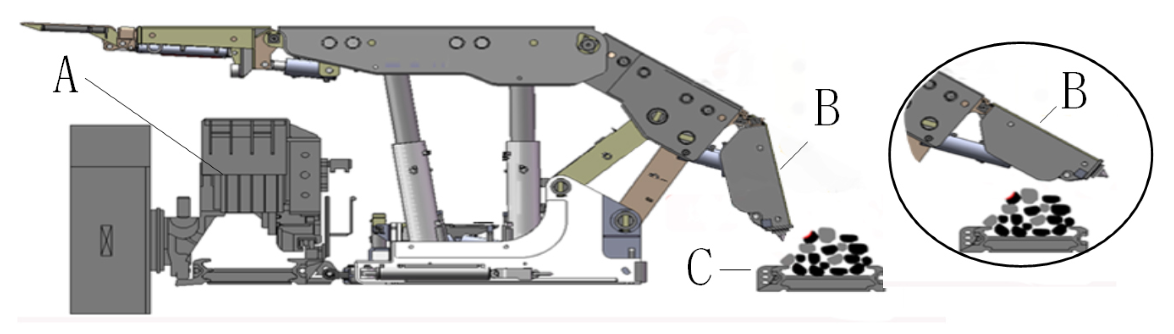
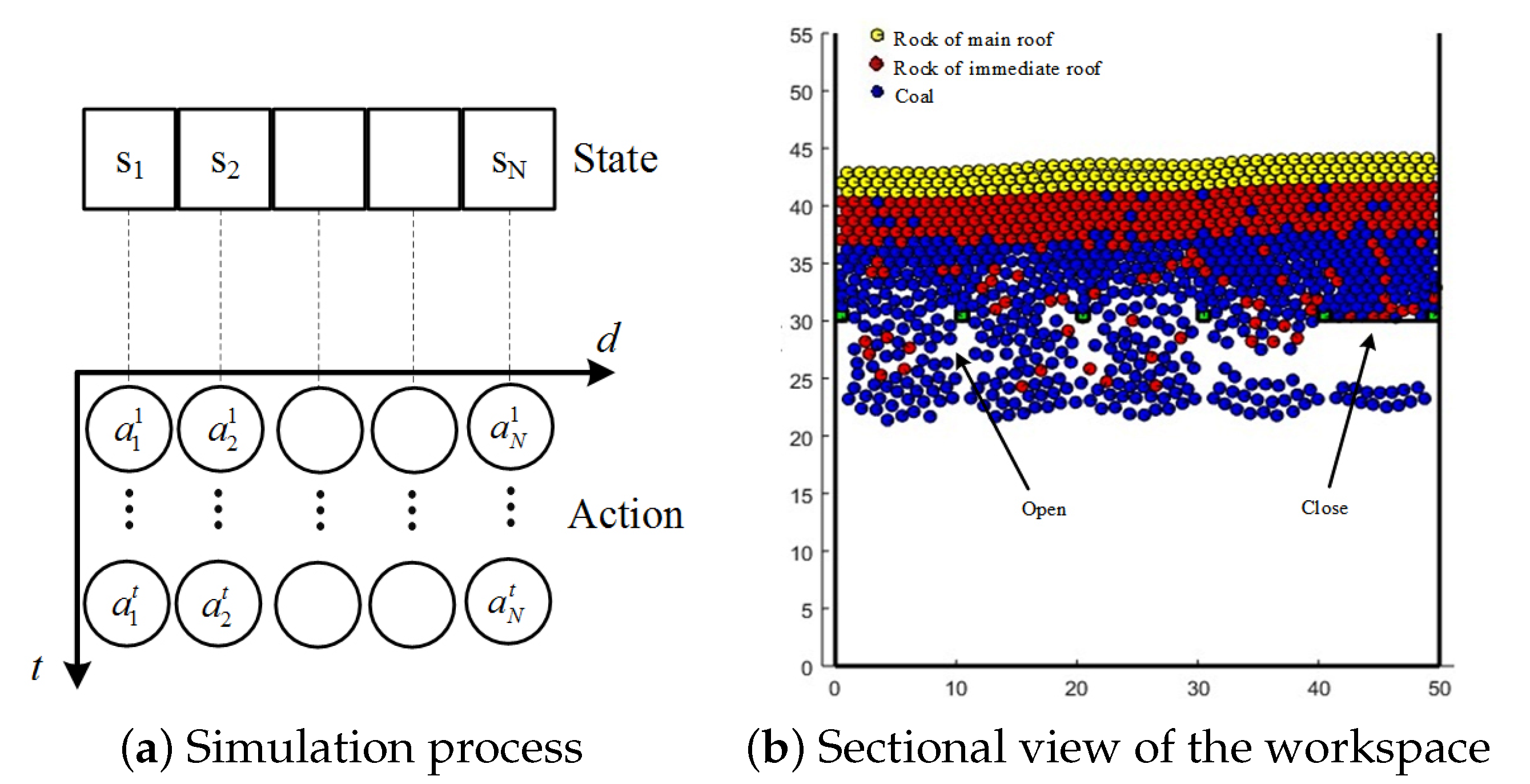
5.1. Top-Coal Caving Simulation Platform

Coal is one of the most important energy sources at present. Currently, top-coal caving is the most efficient method for mining the thick coal seam underground, as shown in Figure 1, the hundreds of hydraulic supports (HSs) are the key equipment for roof supporting and top-coal mining.

The top-coal mining sequence functions as follows: the shearer cuts coal in the coal wall, then the tail boom of HSs opens to captures the falling coal. In this process, the tail boom action is the key of HSs to exploit the maximum top-coal with minimum rocks. Hence, the tail boom acts as a window, it will open when the top-coal falling, while they will close to prevent the rock falling into the drag conveyor if all the top-coal has been captured [47,51,52]. However, it is hard to obtain a perfect performance by operating HSs individually [52]. Hence, considering the window of HSs as a multi-agent system is a direct choice to improve the top-coal mining performance.

In this paper, we employ the simulation platform developed by ourselves based on DICE [53] to validate the proposed method. The DICE system is an open source system to simulate a complicated dynamic process and interaction of discrete elements [54]. Our code [47] can be found in github (https://github.com/YangYi-HPU/Reinforcement-learning-simulation-environment-for-top-coal-caving accessed on 2 December 2019).

The Markov process of top-coal caving is shown in Figure 2a. Based on the Markov model, the top-coal caving dynamic is shown in Figure 2b. In this platform, there are five windows opening and closing to obtain and prevent the particles falling. The particles above the windows consist of three kinds: coal, rock from the immediate-roof, and rock from the main-roof [47].

5.2. Top-Coal Caving Decision Experiment Based on OEAN

In this experiment, the action space of HSs is set as $\mathcal{A}=\left\{{\tilde{a}}_1,{\tilde{a}}_2\right\}$, ${\tilde{a}}_1$ and ${\tilde{a}}_2$, respectively, which denote the opened and closed state of the windows. The condition of agent i by ${\overrightarrow{s}}_i$, $i=\left\{1,2\dots ,5\right\}$, if the coal ration near the window is great than 0.5, set ${\overrightarrow{s}}_i=1$, otherwise ${\overrightarrow{s}}_i=0$. Hence, we define the state space of the multi-agent system as $\mathcal{S}=\left\{s_1,\dots ,s_{32}\right\}$, shown in

Table 1. State space of the top-coal caving.

State	${\overrightarrow{\mathit{s}}}_5$	${\overrightarrow{\mathit{s}}}_4$	${\overrightarrow{\mathit{s}}}_3$	${\overrightarrow{\mathit{s}}}_2$	${\overrightarrow{\mathit{s}}}_1$	State	${\overrightarrow{\mathit{s}}}_5$	${\overrightarrow{\mathit{s}}}_4$	${\overrightarrow{\mathit{s}}}_3$	${\overrightarrow{\mathit{s}}}_2$	${\overrightarrow{\mathit{s}}}_1$
$s_1$	0	0	0	0	0	$s_{17}$	0	0	1	1	1
$s_2$	0	0	0	0	1	$s_{18}$	0	1	1	1	0
$s_3$	0	0	0	1	0	$s_{19}$	1	1	1	0	0
$s_4$	0	0	1	0	0	$s_{20}$	0	1	0	1	1
$s_5$	0	1	0	0	0	$s_{21}$	1	0	1	1	0
$s_6$	1	0	0	0	0	$s_{22}$	1	0	0	1	1
$s_7$	0	0	0	1	1	$s_{23}$	0	1	1	0	1
$s_8$	0	0	1	1	0	$s_{24}$	1	1	0	1	0
$s_9$	0	1	1	0	0	$s_{25}$	1	1	0	0	1
$s_{10}$	1	1	0	0	0	$s_{26}$	1	0	1	0	1
$s_{11}$	0	0	1	0	1	$s_{27}$	0	1	1	1	1
$s_{12}$	0	1	0	1	0	$s_{28}$	1	1	1	1	0
$s_{13}$	1	0	1	0	0	$s_{29}$	1	1	1	0	1
$s_{14}$	0	1	0	0	1	$s_{30}$	1	1	0	1	1
$s_{15}$	1	0	0	1	0	$s_{31}$	1	0	1	1	1
$s_{16}$	1	0	0	0	1	$s_{32}$	1	1	1	1	1

.

According to the states defined above, the function of HMRF shown in Equation (20) is given as follows:

$$\begin{array}{c}\hfill f\left(s\mid a_i,N_i\right)=exp\left(-{\sigma }_{a_i}\frac{\left(s-N^{{\mu }_{a_i}}\right)}{\omega }\right)\end{array}$$

(34)

where $\omega$ is a positive constant; ${\mu }_{a_i}$, ${\sigma }_{a_i}$ are variables and formalized as follows:

$${\mu }_{a_i}=\left\{\begin{array}{c}\hfill 1,a_i={\tilde{a}}_1\\ \hfill 0,a_i={\tilde{a}}_2\end{array}\right.$$

(35)

$${\sigma }_{a_i}=\left\{\begin{array}{c}\hfill -1,a_i={\tilde{a}}_1\\ \hfill 1,a_i={\tilde{a}}_2\end{array}\right.$$

(36)

By Equation (23), the optimal action is

$$\begin{array}{c}\hfill \widehat{a}=\underset{a_i,\dots ,a_N}{argmin}\sum _i\left({\sigma }_{a_i}\frac{\left(s-N^{{\mu }_{a_i}}\right)}{\omega }-\beta Q_i^t\left(s,a_i,{\overline{a}}_i^{*}\right)\right)\end{array}$$

(37)

and the OEAN can be calculated by Equation (26).

The reward architecture for reinforcement learning is

$$\begin{array}{c}\hfill R=n_r{r}_r+n_c{r}_c-\tau \end{array}$$

(38)

where $n_r$ is the obtained rock number, $r_r$ is the reward of each rock; $n_c$ is the obtained coal number, $r_c$ is the reward of each coal, $\tau$ is the time constant. The performance indices of top-coal caving experiment are focus on total reward (TR), shown as Equation (38), coal recall (CR) and the rock ratio in all mining (RR) [47].

$$\begin{array}{c}\hfill CR=\frac{n_c}{n_{c\_total}}\\ \hfill RR=\frac{n_r}{n_c+n_r}\end{array}$$

(39)

where $n_{c\_total}$ is the number of all coal particle. In this experiment, we set the parameters as $r_r=-3$, $r_c=1$, $\alpha =0.2$, $\beta =0.1$, $\omega =1$, $\zeta =0.0001$.

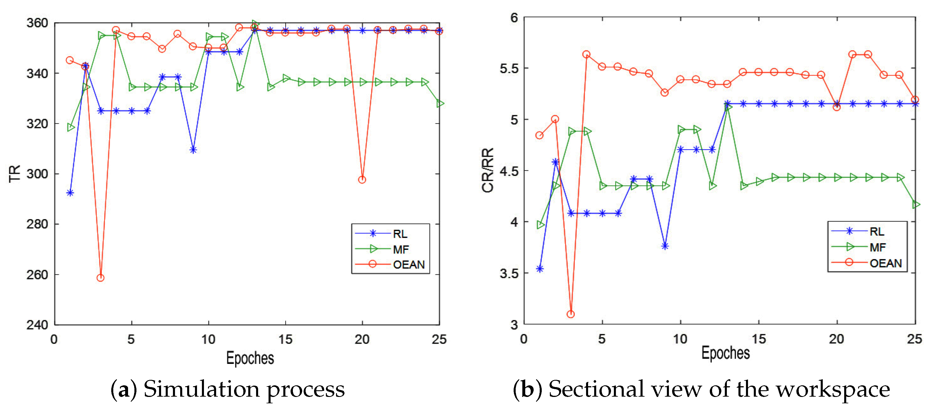
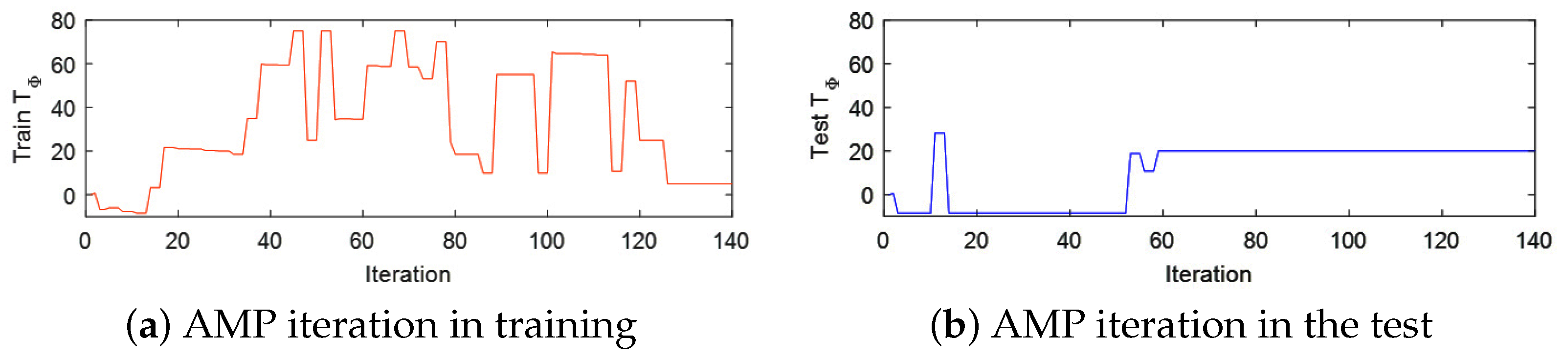
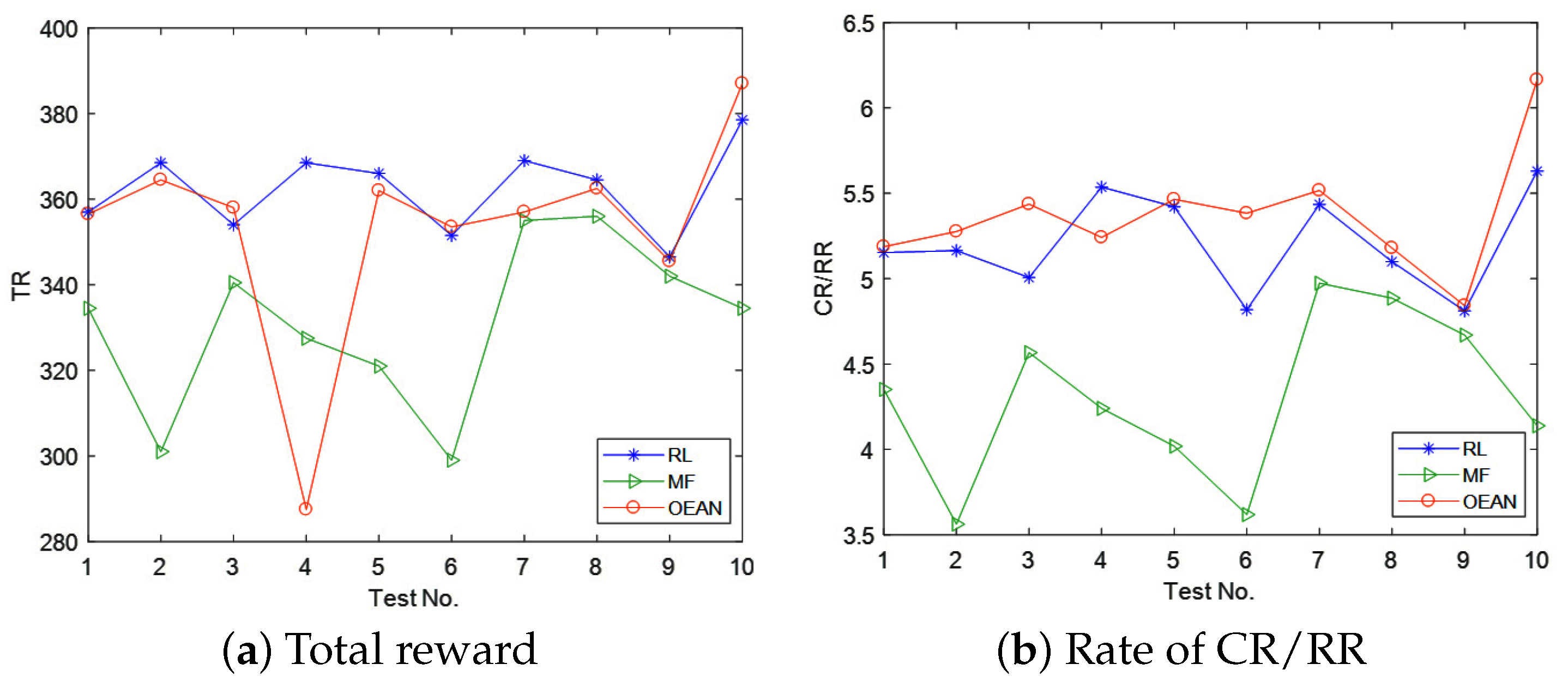
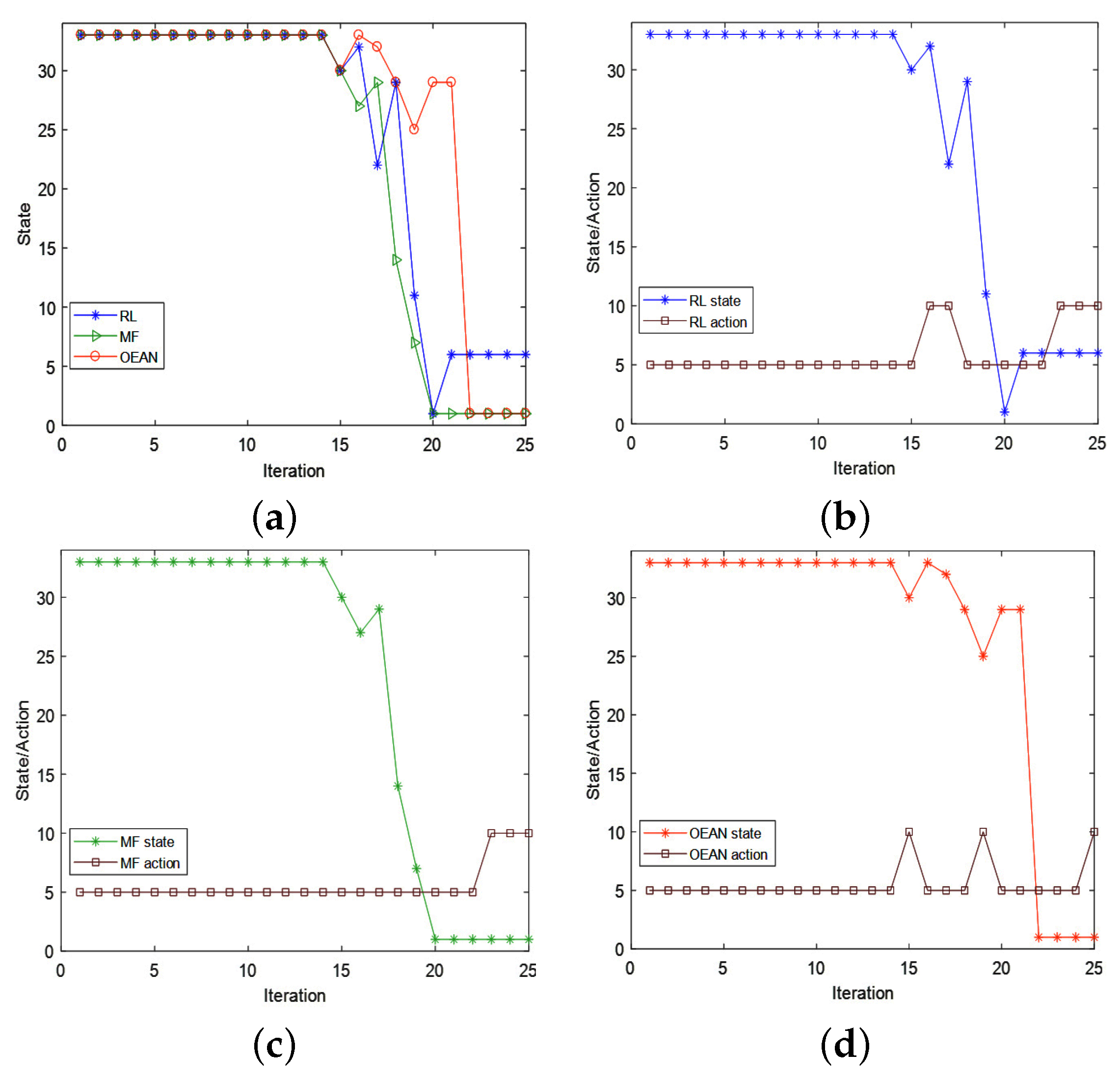
5.3. Experiment Result Analysis

The comparative experiments are carried out in this section. The three methods of multi-agent controlling are employed: independent RL [25], RL with mean field theory [24] and the method proposed in this paper. In the following sections, they are denoted by RL, MF, and OEAN, respectively.

The training and testing processes are alternatively carried out during the model learning. To make the states of each step covering the state space as much as possible, the location of rock particle in the coal layer is set as random.

The TR of test during the model learning are shown in Figure 3a. As we can find out that the TRs increase with the learning process. The RL and OEAN can obtain the highest TR after 15 epochs learning. The OEAN swaying at the end, especially, in 20 epoch, there is a singular point. Although the imperfection of the swaying, the OEAN can obtain the perfect performance in top-coal caving, shown in Figure 3b, and the RR is lower with greater CR.

The dynamic process of MAP obtaining optimal decision is shown in Figure 4. We should note that the environment is changed during the top-coal mining, and $T_{\mathsf{\Phi }}$ converges to the minimum. It is obvious that in the training process, the action decision is produced by $ϵ$-greedy algorithm, and most of them is random, hence it makes the frequent changes in dynamic process of $T_{\mathsf{\Phi }}$. While in the test process, the action is optimal decision by the agent, hence there are few changes in the dynamic process of $T_{\mathsf{\Phi }}$.

After completing the training of Q-value, 10 tests are carried out for validating the method effect. In the tests, the rock particles location in the coal layer are given randomly. The performance indices are shown in

Table 2. Performance index of top-coal caving.

No.	CR			RR
	RL	MF	OEAN	RL	MF	OEAN
1	0.90	0.94	0.91	0.17	0.23	0.18
2	0.94	0.96	0.92	0.18	0.27	0.17
3	0.91	0.92	0.89	0.18	0.19	0.16
4	0.90	0.93	0.66	0.16	0.19	0.13
5	0.93	0.95	0.91	0.17	0.24	0.17
6	0.92	0.94	0.89	0.19	0.23	0.17
7	0.93	0.92	0.89	0.17	0.17	0.16
8	0.94	0.94	0.92	0.18	0.19	0.18
9	0.92	0.93	0.92	0.19	0.2	0.19
10	0.93	0.94	0.93	0.17	0.19	0.15

and Figure 5.

According to Figure 5a the TR of RL and OEAN can approach a high level, and in Figure 5b, the rate of CR to RR shows that OEAN could obtain the most performance of top-coal caving. Especially in the Tests No. 1, 3, 6, 9, and 10, the total reward and rate of CR to RR are the best if the OEAN is employed. That indicates in those tests, the OEAN method could obtain the global optimal decision. In the other tests of adopting the OEAN, although the total reward cannot approach the optimum level, the rate of CR to RR is the best. That means the OEAN method can obtain a better pose between the coal recall and rock ratio in the top-coal caving.

To analyze the details of optimal decision making, we chose the middle window in Test 10 to show the states and actions in the complete process of top-coal caving. The results are shown in Figure 6. Before the 15th iteration, the actions and states of the three methods are the same. Subsequently, the shearer approached the boundary of coal layer and rock layer. In this stage, the RL and MF method just close the window, while the OEAN method regulates the window switching close and open. Therefore the system state changes slowly, and the agent can obtain better performance of the top-coal caving.

6. Conclusions

This paper proposes a new action value function of reinforcement learning-based OEAN for multi-agent system to approach the optimal decision. The new Q-value function contains the relationship between the current agent and its OEAN, and the proposed OEAN makes the communication between the agents simple and direct. The effectiveness of this method is validated by a case study of top-coal caving. The experiment results show that our method improves the training process of RL and obtains a better reward compared with the other two methods. For the top-coal caving, our method can decrease the rock ratio in the mining and relieves the conflict between RR and CR.

In future, we will extend to the following two research topics to improve the performance of top-coal caving.

(1) The agent state of this paper depicts the global environment, hence the dimension of state space is great. If the number of multi-agents is huge, there needs to be a vast state space to describe the environment more detail. In the future, the local state of environment will be researched to decrease the state space dimension and improve the performance of the RL for multi-agent.

(2) The relationship between current agent and its neighbors is depicted by the HMRF model, and an explicit formula is used to establish the HMRF model. Hence, the generalization of the HMRF model is imperfect. In future work, the graph network based on OEAN will be employed to depict the relationship of multi-agent.

References

1. Qian, W.; Xing, W.; Fei, S. H infinity state estimation for neural networks with general activation function and mixed time-varying delays. IEEE Trans. Neural Netw. Learn. Syst. 2020, 32, 3909–3918. [Google Scholar] [CrossRef] [PubMed]
2. Ren, Y.; Zhao, Z.; Zhang, C.; Yang, Q.; Hong, K.S. Adaptive neural-network boundary control for a flexible manipulator with input constraints and model uncertainties. IEEE Trans. Cybern. 2020, 51, 4796–4807. [Google Scholar] [CrossRef] [PubMed]
3. Liu, C.; Wen, G.; Zhao, Z.; Sedaghati, R. Neural-network-based sliding-mode control of an uncertain robot using dynamic model approximated switching gain. IEEE Trans. Cybern. 2020, 51, 2339–2346. [Google Scholar] [CrossRef]
4. Zhao, Z.; Ren, Y.; Mu, C.; Zou, T.; Hong, K.S. Adaptive neural-network-based fault-tolerant control for a flexible string with composite disturbance observer and input constraints. IEEE Trans. Cybern. 2021, 1–11. [Google Scholar] [CrossRef] [PubMed]
5. Jiang, Y.; Wang, Y.; Miao, Z.; Na, J.; Zhao, Z.; Yang, C. Composite-learning-based adaptive neural control for dual-arm robots with relative motion. IEEE Trans. Neural Netw. Learn. Syst. 2020, 33, 1010–1021. [Google Scholar] [CrossRef]
6. Qian, W.; Li, Y.; Chen, Y.; Liu, W. L2-L infinity filtering for stochastic delayed systems with randomly occurring nonlinearities and sensor saturation. Int. J. Syst. Sci. 2020, 51, 2360–2377. [Google Scholar] [CrossRef]
7. Sutton, R.S.; Barto, A.G. Reinforcement Learning: An Introduction; MIT Press: Cambridge, MA, USA, 2018. [Google Scholar]
8. Lan, X.; Liu, Y.; Zhao, Z. Cooperative control for swarming systems based on reinforcement learning in unknown dynamic environment. Neurocomputing 2020, 410, 410–418. [Google Scholar] [CrossRef]
9. Bellman, R. Dynamic programming. Science 1966, 153, 34–37. [Google Scholar] [CrossRef]
10. Luo, B.; Liu, D.; Huang, T.; Wang, D. Model-Free Optimal Tracking Control via Critic-Only Q-Learning. IEEE Trans. Neural Netw. Learn. Syst. 2016, 27, 2134–2144. [Google Scholar] [CrossRef]
11. Qian, W.; Gao, Y.; Yang, Y. Global consensus of multiagent systems with internal delays and communication delays. IEEE Trans. Syst. Man Cybern. Syst. 2018, 49, 1961–1970. [Google Scholar] [CrossRef]
12. Wei, Q.; Kasabov, N.; Polycarpou, M.; Zeng, Z. Deep learning neural networks: Methods, systems, and applications. Neurocomputing 2020, 396, 130–132. [Google Scholar] [CrossRef]
13. Liu, Z.; Shi, J.; Zhao, X.; Zhao, Z.; Li, H.X. Adaptive Fuzzy Event-triggered Control of Aerial Refueling Hose System with Actuator Failures. IEEE Trans. Fuzzy Syst. 2021, 1. [Google Scholar] [CrossRef]
14. Qian, W.; Li, Y.; Zhao, Y.; Chen, Y. New optimal method for L2-L infinity state estimation of delayed neural networks. Neurocomputing 2020, 415, 258–265. [Google Scholar] [CrossRef]
15. Lowe, R.; Wu, Y.; Tamar, A.; Harb, J.; Abbeel, O.P.; Mordatch, I. Multi-agent actor-critic for mixed cooperative-competitive environments. In Proceedings of the Advances in Neural Information Processing Systems, Long Beach, CA, USA, 4–8 December 2017; pp. 6379–6390. [Google Scholar]
16. Matta, M.; Cardarilli, G.C.; Di Nunzio, L.; Fazzolari, R.; Giardino, D.; Re, M.; Silvestri, F.; Spanò, S. Q-RTS: A real-time swarm intelligence based on multi-agent Q-learning. Electron. Lett. 2019, 55, 589–591. [Google Scholar] [CrossRef]
17. Sadhu, A.K.; Konar, A. Improving the speed of convergence of multi-agent Q-learning for cooperative task-planning by a robot-team. Robot. Auton. Syst. 2017, 92, 66–80. [Google Scholar] [CrossRef]
18. Ni, Z.; Paul, S. A Multistage Game in Smart Grid Security: A Reinforcement Learning Solution. IEEE Trans. Neural Netw. Learn. Syst. 2019, 30, 2684–2695. [Google Scholar] [CrossRef]
19. Sun, C.; Karlsson, P.; Wu, J.; Tenenbaum, J.B.; Murphy, K. Stochastic prediction of multi-agent interactions from partial observations. arXiv 2019, arXiv:1902.09641. [Google Scholar]
20. Mo, X.; Huang, Z.; Xing, Y.; Lv, C. Multi-agent trajectory prediction with heterogeneous edge-enhanced graph attention network. IEEE Trans. Intell. Transp. Syst. 2022, 1–14. [Google Scholar] [CrossRef]
21. Niu, Y.; Paleja, R.; Gombolay, M. Multi-agent graph-attention communication and teaming. In Proceedings of the 20th International Conference on Autonomous Agents and MultiAgent Systems, Online, 3–7 May 2021; pp. 964–973. [Google Scholar]
22. Koller, D.; Friedman, N.; Bach, F. Probabilistic Graphical Models: Principles and Techniques; MIT Press: Cambridge, MA, USA, 2009. [Google Scholar]
23. Sadhu, A.K.; Konar, A. An Efficient Computing of Correlated Equilibrium for Cooperative Q-Learning-Based Multi-Robot Planning. IEEE Trans. Syst. Man, Cybern. Syst. 2018, 8, 2779–2794. [Google Scholar] [CrossRef]
24. Yang, Y.; Rui, L.; Li, M.; Ming, Z.; Wang, J. Mean Field Multi-Agent Reinforcement Learning. arXiv 2018, arXiv:1802.05438. [Google Scholar]
25. Matignon, L.; Laurent, G.J.; Le Fort-Piat, N. Independent reinforcement learners in cooperative markov games: A survey regarding coordination problems. Knowl. Eng. Rev. 2012, 27, 1–31. [Google Scholar] [CrossRef] [Green Version]
26. Buşoniu, L.; Babuška, R.; De Schutter, B. Multi-agent reinforcement learning: An overview. In Innovations in Multi-Agent Systems and Applications-1; Springer: Berlin/Heidelberg, Germany, 2010; pp. 183–221. [Google Scholar]
27. Shoham, Y.; Powers, R.; Grenager, T. If multi-agent learning is the answer, what is the question? Artif. Intell. 2007, 171, 365–377. [Google Scholar] [CrossRef] [Green Version]
28. Littman, M.L. Value-function reinforcement learning in Markov games. Cogn. Syst. Res. 2001, 2, 55–66. [Google Scholar] [CrossRef] [Green Version]
29. Hu, J.; Wellman, M.P. Nash Q-Learning for General-Sum Stochastic Games. J. Mach. Learn. Res. 2003, 4, 1039–1069. [Google Scholar]
30. Hu, J.; Wellman, M.P. Multiagent reinforcement learning: Theoretical framework and an algorithm. In Proceedings of the ICML, Madison, WI, USA, 24–27 July 1998; Volume 98, pp. 242–250. [Google Scholar]
31. Jaakkola, T.; Jordan, M.I.; Singh, S.P. Convergence of Stochastic Iterative Dynamic Programming Algorithms. Neural Comput. 1993, 6, 1185–1201. [Google Scholar] [CrossRef] [Green Version]
32. Molina, J.P.; Zolezzi, J.M.; Contreras, J.; Rudnick, H.; Reveco, M.J. Nash-Cournot Equilibria in Hydrothermal Electricity Markets. IEEE Trans. Power Syst. 2011, 26, 1089–1101. [Google Scholar] [CrossRef]
33. Yang, L.; Sun, Q.; Ma, D.; Wei, Q. Nash Q-learning based equilibrium transfer for integrated energy management game with We-Energy. Neurocomputing 2019, 396, 216–223. [Google Scholar] [CrossRef]
34. Vamvoudakis, K.G. Non-zero sum Nash Q-learning for unknown deterministic continuous-time linear systems. Automatica 2015, 61, 274–281. [Google Scholar] [CrossRef]
35. Levine, S. Reinforcement learning and control as probabilistic inference: Tutorial and review. arXiv 2018, arXiv:1805.00909. [Google Scholar]
36. Chalkiadakis, G.; Boutilier, C. Coordination in multiagent reinforcement learning: A Bayesian approach. In Proceedings of the Second International Joint Conference on Autonomous Agents and Multiagent Systems, Melbourne, Australia, 14–18 July 2003; pp. 709–716. [Google Scholar]
37. Teacy, W.L.; Chalkiadakis, G.; Farinelli, A.; Rogers, A.; Jennings, N.R.; McClean, S.; Parr, G. Decentralized Bayesian reinforcement learning for online agent collaboration. In Proceedings of the 11th International Conference on Autonomous Agents and Multiagent Systems-Volume 1. International Foundation for Autonomous Agents and Multiagent Systems, Valencia, Spain, 4–8 June 2012; pp. 417–424. [Google Scholar]
38. Chalkiadakis, G. A Bayesian Approach to Multiagent Reinforcement Learning and Coalition Formation under Uncertainty; University of Toronto: Toronto, ON, Canda, 2007. [Google Scholar]
39. Zhang, X.; Aberdeen, D.; Vishwanathan, S. Conditional random fields for multi-agent reinforcement learning. In Proceedings of the 24th International Conference on Machine Learning, Corvalis, OR, USA, 20–24 June 2007; pp. 1143–1150. [Google Scholar]
40. Handa, H. EDA-RL: Estimation of distribution algorithms for reinforcement learning problems. In Proceedings of the 11th Annual Conference on Genetic and Evolutionary Computation, Montreal, QC, Canada, 8–12 July 2009; pp. 405–412. [Google Scholar]
41. Daniel, C.; Van Hoof, H.; Peters, J.; Neumann, G. Probabilistic inference for determining options in reinforcement learning. Mach. Learn. 2016, 104, 337–357. [Google Scholar] [CrossRef] [Green Version]
42. Dethlefs, N.; Cuayáhuitl, H. Hierarchical reinforcement learning and hidden Markov models for task-oriented natural language generation. In Proceedings of the 49th Annual Meeting of the Association for Computational Linguistics: Human Language Technologies: Short Papers-Volume 2, Association for Computational Linguistics, Portland, OR, USA, 19–24 June 2011; pp. 654–659. [Google Scholar]
43. Sallans, B.; Hinton, G.E. Reinforcement learning with factored states and actions. J. Mach. Learn. Res. 2004, 5, 1063–1088. [Google Scholar]
44. Zhang, Y.; Brady, M.; Smith, S. Segmentation of brain MR images through a hidden Markov random field model and the expectation-maximization algorithm. IEEE Trans. Med. Imaging 2001, 20, 45–57. [Google Scholar] [CrossRef] [PubMed]
45. Chatzis, S.P.; Tsechpenakis, G. The infinite hidden Markov random field model. IEEE Trans. Neural Networks 2010, 21, 1004–1014. [Google Scholar] [CrossRef] [PubMed]
46. Littman, M.L.; Stone, P. A polynomial-time Nash equilibrium algorithm for repeated games. Decis. Support Syst. 2005, 39, 55–66. [Google Scholar] [CrossRef]
47. Yang, Y.; Lin, Z.; Li, B.; Li, X.; Cui, L.; Wang, K. Hidden Markov random field for multi-agent optimal decision in top-coal caving. IEEE Access 2020, 8, 76596–76609. [Google Scholar] [CrossRef]
48. Moon, T.K. The expectation-maximization algorithm. IEEE Signal Process. Mag. 1996, 13, 47–60. [Google Scholar] [CrossRef]
49. Wang, Q. HMRF-EM-image: Implementation of the Hidden Markov Random Field Model and its Expectation-Maximization Algorithm. Comput. Sci. 2012, 94, 222–233. [Google Scholar]
50. Szepesvári, C.; Littman, M.L. A unified analysis of value-function-based reinforcement- learning algorithms. Neural Comput. 1999, 11, 2017–2059. [Google Scholar] [CrossRef]
51. Vakili, A.; Hebblewhite, B.K. A new cavability assessment criterion for Longwall Top Coal Caving. Int. J. Rock Mech. Min. Sci. 2010, 47, 1317–1329. [Google Scholar] [CrossRef]
52. Liu, C.; Li, H.; Mitri, H. Effect of Strata Conditions on Shield Pressure and Surface Subsidence at a Longwall Top Coal Caving Working Face. Rock Mech. Rock Eng. 2019, 52, 1523–1537. [Google Scholar] [CrossRef]
53. Zhao, G. DICE2D an Open Source DEM. Available online: http://www.dembox.org/ (accessed on 15 June 2017).
54. Sapuppo, F.; Schembri, F.; Fortuna, L.; Llobera, A.; Bucolo, M. A polymeric micro-optical system for the spatial monitoring in two-phase microfluidics. Microfluid. Nanofluidics 2012, 12, 165–174. [Google Scholar] [CrossRef]
Figure 1. Top-coal caving process. A: Shearer, B: Tail boom of a hydraulic support, it acts as a window open and close. C: Drag conveyor. When the window is opened, the top-coal will collapse and be captured by the drag conveyor. In the sub-graph, the window is closed to prevent the rock falling down.
Actuators 11 00099 g001
Figure 2. Simulation platform of top-coal caving. In (a), The s i , a i t , respectively, denote the state and action of agent i on the time point t. In (b), a number of rock and coal particles distribute randomly in the boundary of rock and coal. Our aim is to obtain the maximum coal with minimum rock by opening and closing the windows.
Actuators 11 00099 g002
Figure 3. Performance indies of test process during the learning process. (a) is the total reward of the three methods. (b) is the ration of the ratio of CR to RR. As we can find out, the convergent tendency of the three methods is obvious in the two sub-figures. The TR is increased with the training process of the three method, and HMRF obtain best TR and the performance of the top-coal caving.
Actuators 11 00099 g003
Figure 4. T Φ dynamic during AMP iterating. It indicts the process of optimal decision making for the neighbourhood by MAP. If the change rate of T Φ closes to zero, MAP obtains the OEAN.
Actuators 11 00099 g004
Figure 5. Tests result with the random location of the rock particles in the coal layer. (a) is the total reward of the three methods. (b) is the rate of CR to RR.
Actuators 11 00099 g005
Figure 6. Tests result with the random location of the rock particles in the coal layer. (a) is the states of three methods. (b) is the states and actions of RL. (c) is the states and actions of MF. (d) is the states and actions of OEAN.
Actuators 11 00099 g006