
What Works? How Combining Equal Opportunity and Work–Life Measures Relates to the Within-Firm Gender Wage Gap


Abstract
:1. Introduction
2. Human Resource Management: The Role of Equal Opportunity and Work–Life Measures
2.1. Comprehensive Personnel Policies as Support against Gender Inequality in Wages
2.2. Personnel Policies as a Separation Strategy and Compensating Differentials
3. Data and Methods
3.1. Data
3.2. Measures
3.3. Methods and Analytical Strategy
4. Results
4.1. Descriptives

| Men (N = 3513) | Women (N = 2926) | t-Test | |||
|---|---|---|---|---|---|
| Mean | SD | Mean | SD | ||
| Log hourly wages | 3.21 | (0.46) | 2.95 | (0.39) | *** |
| Hourly wages in Euro | 27.96 | (24.41) | 20.77 | (10.55) | *** |
| Human capital characteristics | |||||
| Age | 40.73 | (8.86) | 40.55 | (8.86) | |
| Age2 | 1737.59 | (686.57) | 1722.64 | (688.00) | |
| Qualification | |||||
| Without vocational training | 0.03 | (0.16) | 0.03 | (0.18) | * |
| With vocational training | 0.63 | (0.48) | 0.64 | (0.48) | |
| Tertiary degree | 0.35 | (0.48) | 0.33 | (0.47) | |
| Labor market experience | 17.66 | (8.71) | 15.55 | (7.85) | *** |
| Labor market experience2 | 387.65 | (321.54) | 303.22 | (266.09) | *** |
| Employment characteristics | |||||
| Occupation | |||||
| Managers | 0.04 | (0.20) | 0.01 | (0.10) | *** |
| Professionals | 0.24 | (0.43) | 0.20 | (0.40) | *** |
| Technicians, associate professional | 0.23 | (0.42) | 0.39 | (0.49) | *** |
| Clerical support workers | 0.11 | (0.32) | 0.21 | (0.41) | *** |
| Services and sales workers | 0.05 | (0.23) | 0.10 | (0.29) | *** |
| Skilled Agricultural | 0.003 | (0.051) | 0.002 | (0.045) | |
| Craft and Related Trades Workers | 0.17 | (0.37) | 0.02 | (0.13) | *** |
| Plant, Machine Operators & Assemblers | 0.10 | (0.30) | 0.02 | (0.14) | *** |
| Elementary occupations | 0.06 | (0.23) | 0.06 | (0.23) | |
| Firm tenure | 8.58 | (7.83) | 7.83 | (7.27) | *** |
| Supervisory responsibility | 0.43 | (0.50) | 0.27 | (0.44) | *** |
| Contractual work hours | 37.89 | (3.78) | 32.18 | (8.53) | *** |
| Overwork hours | 5.65 | (7.14) | 4.74 | (6.73) | *** |
| Family characteristics | |||||
| Age of the youngest child | 11.64 | (5.99) | 13.42 | (6.59) | *** |
| Number of children | |||||
| No child | 0.35 | (0.48) | 0.34 | (0.47) | |
| 1–2 children | 0.52 | (0.50) | 0.57 | (0.50) | *** |
| 3 and more children | 0.14 | (0.34) | 0.10 | (0.29) | *** |
| Partner | 0.85 | (0.36) | 0.83 | (0.37) | * |
| Measures | Mean | SD | Min | Max |
|---|---|---|---|---|
| Equal opportunity | ||||
| Mentoring | 0.41 | 0.49 | 0 | 1 |
| Women’s quota | 0.27 | 0.44 | 0 | 1 |
| Mixed teams | 0.22 | 0.41 | 0 | 1 |
| Work–Life | ||||
| Childcare support | 0.53 | 0.50 | 0 | 1 |
| Support for parental leavers | 0.77 | 0.42 | 0 | 1 |
| Flexible working hours (org.) | 0.95 | 0.21 | 0 | 1 |
| Awareness flex. hours (agg.) | 0.63 | 0.38 | 0 | 1 |
| Home-based telework | 0.62 | 0.49 | 0 | 1 |
| Sum of equal opportunity measures | 0.89 | 0.96 | 0 | 3 |
| Sum of work-life measures | 2.88 | 0.92 | 0 | 4 |
| Sum of all measures | 3.77 | 1.54 | 0 | 7 |
4.2. Impact of Equal Opportunity and Work–Life Measures on the GWG
| (1) | (2) | (3) | (4) | |
|---|---|---|---|---|
| Overall | Low/Medium Qualification | High Qualification | Parents | |
| Step 1:GWG only | ||||
| Women | −0.1147 *** | −0.1252 *** | −0.0837 *** | −0.1536 *** |
| (0.0116) | (0.0128) | (0.0203) | (0.0153) | |
| Constant | 2.8910 *** | 2.8133 *** | 2.4260 *** | 3.0729 *** |
| (0.1217) | (0.1426) | (0.2596) | (0.2181) | |
| Step 2: Equal opportunity measures | ||||
| Women | −0.1260 *** | −0.1237 *** | −0.1044 ** | −0.1568 *** |
| (0.0150) | (0.0156) | (0.0311) | (0.0210) | |
| Mentoringxwomen | −0.0022 | −0.0169 | −0.0119 | −0.0233 |
| (0.0257) | (0.0320) | (0.0401) | (0.0340) | |
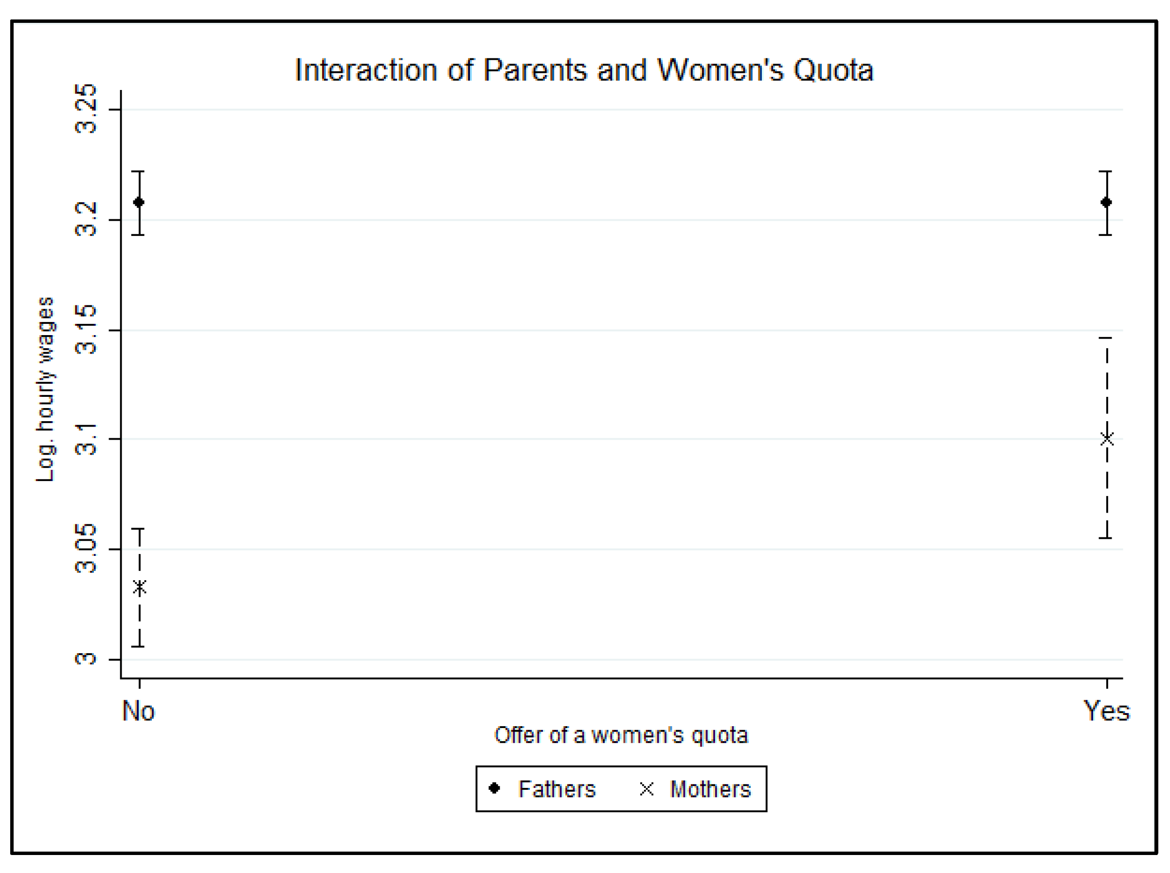
| Women’s quotaxwomen | 0.0492 | 0.0257 | 0.0773 | 0.0676 * |
| (0.0253) | (0.0315) | (0.0394) | (0.0324) | |
| Mixed teamsxwomen | −0.0128 | −0.0094 | −0.0079 | −0.0349 |
| (0.0276) | (0.0291) | (0.0411) | (0.0374) | |
| Constant | 2.8884 *** | 2.8113 *** | 2.4189 *** | 3.0775 *** |
| (0.1222) | (0.1427) | (0.2598) | (0.2192) | |
| Step 3: Work–Life measures | ||||
| Women | −0.0996 ** | −0.0874 ** | −0.1325 * | −0.1460 ** |
| (0.0341) | (0.0329) | (0.0635) | (0.0420) | |
| Childcare supportxwomen | −0.0491 * | −0.0134 | −0.0570 | −0.0778 ** |
| (0.0214) | (0.0233) | (0.0378) | (0.0286) | |
| Support for parental leaversxwomen | 0.0052 | −0.0032 | 0.0053 | 0.0049 |
| (0.0290) | (0.0310) | (0.0385) | (0.0355) | |
| Home-based teleworkxwomen | 0.0065 | 0.0067 | −0.0218 | 0.0020 |
| (0.0239) | (0.0250) | (0.0439) | (0.0333) | |
| Flexible work hoursxwomen | 0.0006 | −0.0053 | 0.0127 | 0.0045 |
| (0.0029) | (0.0028) | (0.0068) | (0.0038) | |
| Constant | 2.8649 *** | 2.7679 *** | 2.4615 *** | 3.0495 *** |
| (0.1238) | (0.1455) | (0.2690) | (0.2187) | |
| N | 6439 | 4266 | 2173 | 4238 |
4.3. From Single Measures to Personnel Strategies
| (1) Overall | (2) Low/Medium Qualifiation | (3) High Qualification | (4) Parents | |
|---|---|---|---|---|
| Step 1: Equal opportunity measures | ||||
| Women | −0.1173 *** | −0.1190 *** | −0.0952 *** | −0.1516 *** |
| (0.0134) | (0.0149) | (0.0240) | (0.0186) | |
| 2 to 3 measuresxwomen | 0.0087 | −0.0231 | 0.0331 | −0.0063 |
| (0.0238) | (0.0234) | (0.0384) | (0.0301) | |
| Constant | 2.8910 *** | 2.8123 *** | 2.4258 *** | 3.0729 *** |
| (0.1217) | (0.1426) | (0.2589) | (0.2180) | |
| Step 2: Work–life measures | ||||
| Women | −0.0670 * | −0.0781 ** | −0.0362 | −0.0665 * |
| (0.0314) | (0.0243) | (0.1065) | (0.0317) | |
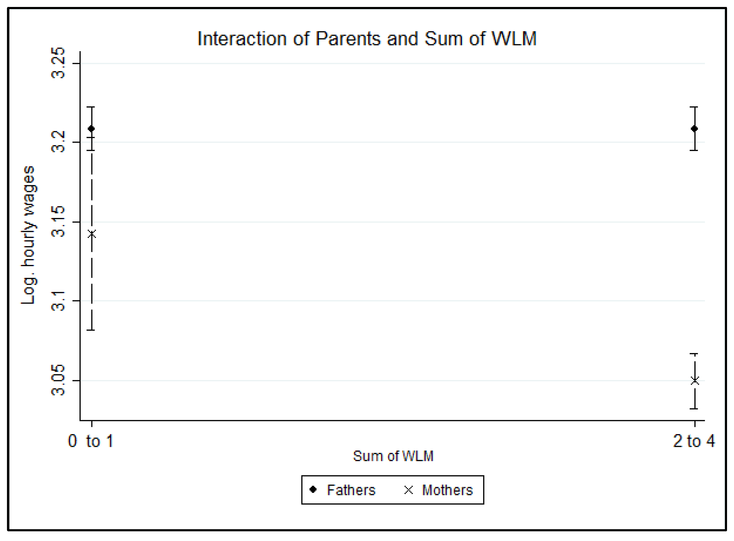
| 2 to 4 measuresxwomen | −0.0508 | −0.0514 | −0.0490 | −0.0925 ** |
| (0.0339) | (0.0277) | (0.1083) | (0.0343) | |
| Constant | 2.8945 *** | 2.8175 *** | 2.4257 *** | 3.0763 *** |
| (0.1220) | (0.1429) | (0.2601) | (0.2193) | |
| N | 6439 | 4266 | 2173 | 4238 |
| Without Equal Opportunity Measures | With at Least One Equal Opportunity Measure | |||||||
|---|---|---|---|---|---|---|---|---|
| (1) | (2) | (3) | (4) | (5) | (6) | (7) | (8) | |
| Overall | Low/Medium Qualification | High Qualification | Parents | Overall | Low/Medium Qualification | High Qualification | Parents | |
| Step 1:Single WLM measures | ||||||||
| Women | −0.1212 *** | −0.1186 ** | −0.1174 | −0.1778 *** | 0.0221 | 0.0529 | −0.0464 | −0.0171 |
| (0.0292) | (0.0339) | (0.1284) | (0.0432) | (0.0538) | (0.0639) | (0.0609) | (0.0734) | |
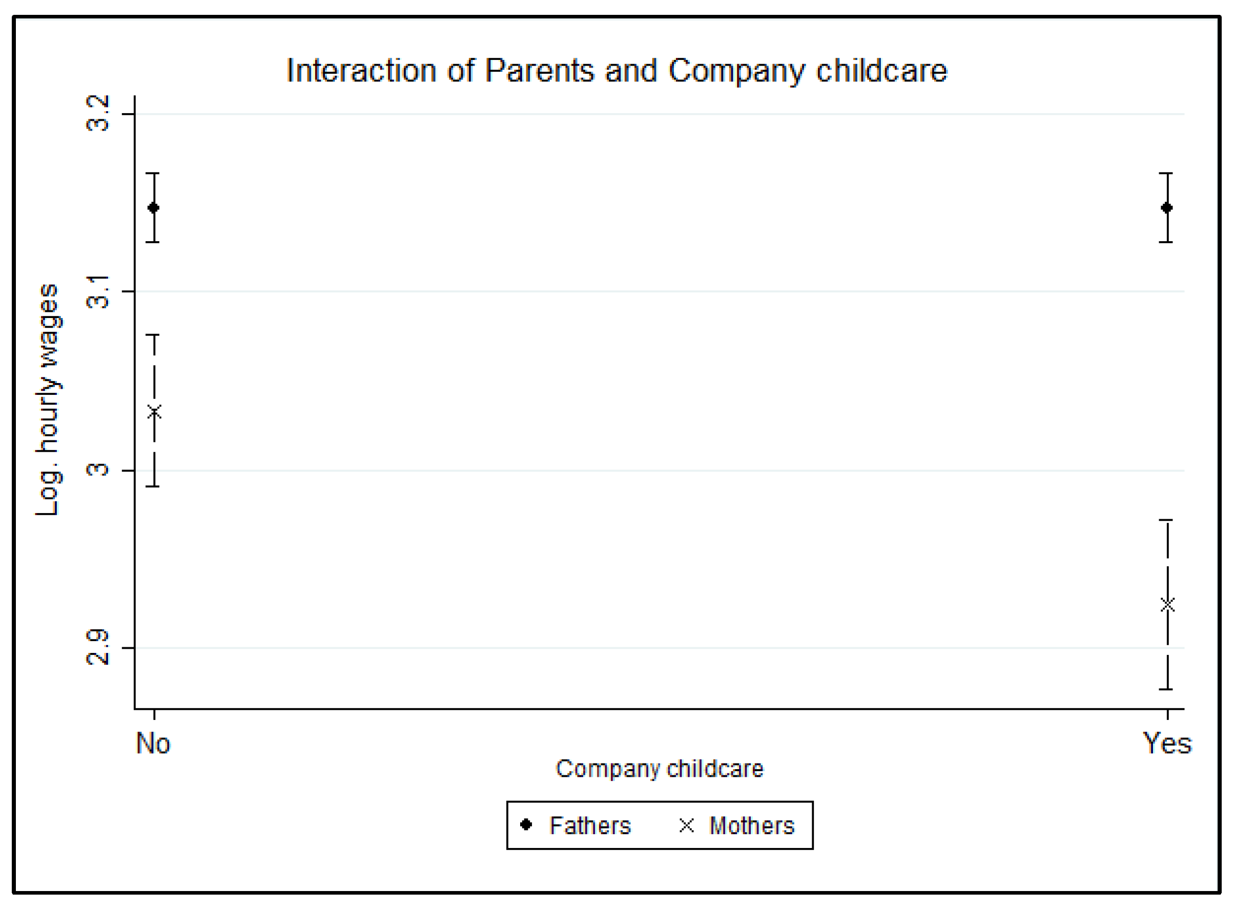
| Childcare supportxwomen | −0.0895 ** | −0.0259 | −0.1287 | −0.1088 ** | −0.0251 | −0.0063 | −0.0297 | −0.0563 |
| (0.0267) | (0.0300) | (0.0714) | (0.0393) | (0.0287) | (0.0323) | (0.0448) | (0.0379) | |
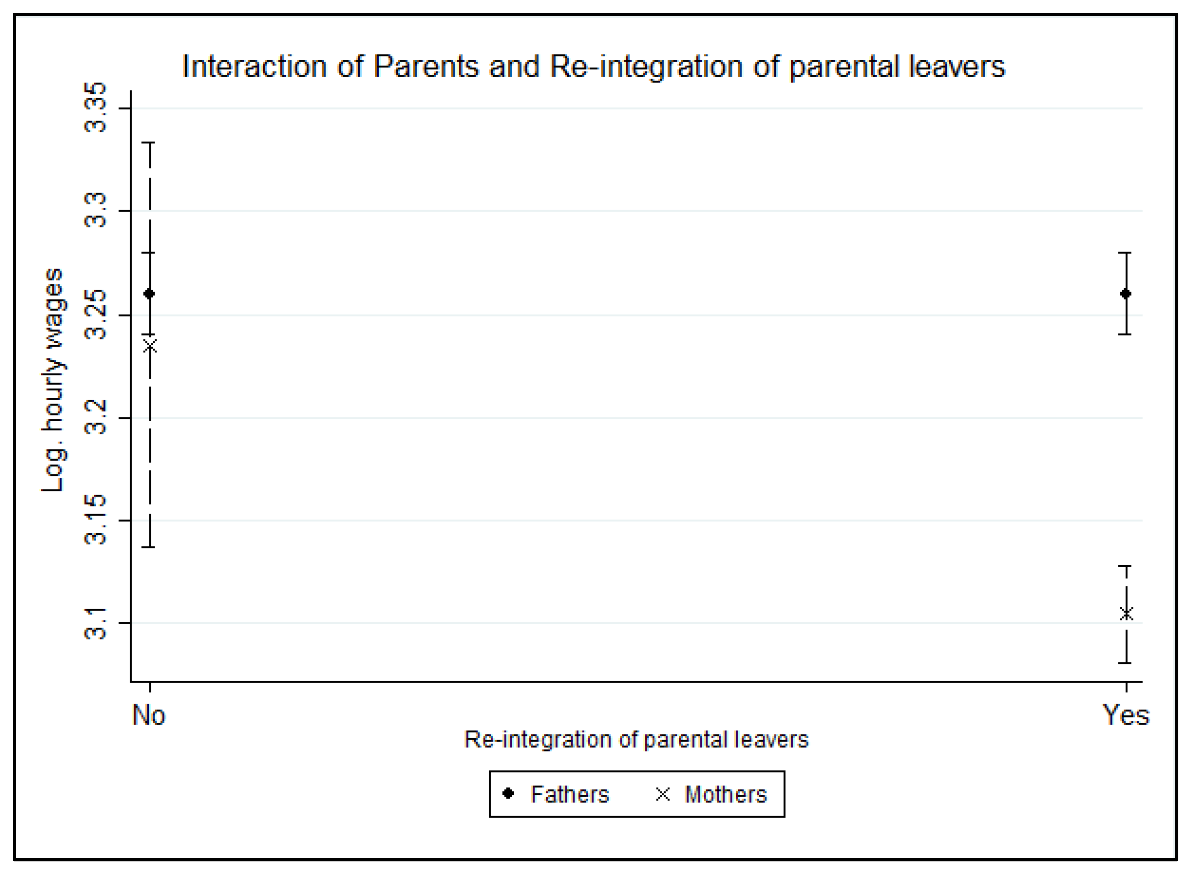
| Support for parental leaversxwomen | 0.0457 (0.0239) | 0.0543 (0.0286) | 0.0126 (0.0659) | 0.0520 (0.0376) | −0.1232 ** (0.0388) | −0.1701 ** (0.0591) | −0.0578 (0.0429) | −0.1309 * (0.0529) |
| Home-based teleworkxwomen | −0.0061 | −0.0055 | −0.0183 | −0.0206 | 0.0037 | 0.0112 | −0.0348 | 0.0092 |
| (0.0317) | (0.0338) | (0.0779) | (0.0464) | (0.0336) | (0.0353) | (0.0494) | (0.0479) | |
| Flexible work hoursxwomen | 0.0011 | −0.0052 | 0.0110 | 0.0070 | 0.0004 | −0.0036 | 0.0101 | 0.0026 |
| (0.0038) | (0.0039) | (0.0116) | (0.0048) | (0.0033) | (0.0035) | (0.0064) | (0.0043) | |
| Constant | 2.8618 *** | 2.7204 *** | 2.5849 *** | 3.1389 *** | 2.8692 *** | 2.8273 *** | 2.2923 *** | 2.9484 *** |
| (0.1987) | (0.2195) | (0.4950) | (0.3022) | (0.1486) | (0.1894) | (0.3173) | (0.3196) | |
| Step 2:Sum of measures | ||||||||
| Women | −0.0987 *** | −0.0968 *** | −0.0873 | −0.1011 *** | 0.0528 | 0.0028 | 0.0653 | 0.0997 |
| (0.0221) | (0.0218) | (0.1550) | (0.0200) | (0.0869) | (0.1038) | (0.0484) | (0.0934) | |
| 2 to 4 measuresxwomen | −0.0368 | −0.0330 | −0.0262 | −0.0700 * | −0.1552 | −0.1273 | −0.1355 * | −0.2478 ** |
| (0.0287) | (0.0283) | (0.1611) | (0.0292) | (0.0875) | (0.1047) | (0.0516) | (0.0924) | |
| Constant | 2.9183 *** | 2.7950 *** | 2.6035 *** | 3.2064 *** | 2.8822 *** | 2.8651 *** | 2.2641 *** | 2.9509 *** |
| (0.1961) | (0.2157) | (0.4667) | (0.3083) | (0.1476) | (0.1895) | (0.3068) | (0.3150) | |
| N | 2920 | 2103 | 817 | 1870 | 3519 | 2163 | 1356 | 2368 |
5. Discussion and Conclusions
Limitations and Further Research
Author Contributions
Funding
Institutional Review Board Statement
Informed Consent Statement
Data Availability Statement
Conflicts of Interest
Appendix A
| Mean | SD | Min | Max | |
|---|---|---|---|---|
| Log hourly wages | 3.09 | (0.45) | 0.54 | 6.54 |
| Hourly wages in Euro | 24.69 | (19.705) | 1.711 | 693.14 |
| Gender | 0.45 | 0.50 | 0 | 1 |
| Human capital characteristics | ||||
| Age | 40.65 | (8.86) | 17 | 54 |
| Age2 | 1730.79 | (687.21) | 289 | 2916 |
| Qualification | ||||
| Without vocational training | 0.03 | (0.17) | 0 | 1 |
| With vocational training | 0.63 | (0.48) | 0 | 1 |
| Tertiary degree | 0.34 | (0.47) | 0 | 1 |
| Labor market experience | 16.70 | (8.39) | 0.50 | 38.36 |
| Labor market experience2 | 349.28 | (321.56) | 0.25 | 1471.20 |
| Employment characteristics | ||||
| Occupation | ||||
| Managers | 0.03 | (0.16) | 0 | 1 |
| Professionals | 0.22 | (0.42) | 0 | 1 |
| Technicians, associate professional | 0.30 | (0.46) | 0 | 1 |
| Clerical support workers | 0.16 | (0.36) | 0 | 1 |
| Services and sales workers | 0.07 | (0.26) | 0 | 1 |
| Skilled Agricultural | 0.002 | (0.05) | 0 | 1 |
| Craft and Related Trades Workers | 0.10 | (0.30) | 0 | 1 |
| Plant & Machine Operators & Assemblers | 0.06 | (0.25) | 0 | 1 |
| Elementary occupations | 0.06 | (0.23) | 0 | 1 |
| Firm tenure | 8.24 | (7.59) | 0.50 | 36.30 |
| Supervisory responsibility | 0.36 | (0.48) | 0 | 1 |
| Contractual work hours | 35.29 | (6.99) | 3 | 50 |
| Overwork hours | 5.24 | (6.97) | −33.5 | 30 |
| Family characteristics | ||||
| Age of the youngest child | 12.447 | (6.33) | 0 | 44 |
| Number of children | ||||
| No child | 0.34 | (0.47) | 0 | 1 |
| 1–2 children | 0.54 | (0.50) | 0 | 1 |
| 3 and more children | 0.12 | (0.32) | 0 | 1 |
| Partner | 0.83 | (0.37) | 0 | 1 |
| N | 6439 |
| b | SE | |
|---|---|---|
| Women (Ref. Men) | −0.1169 *** | 0.0117 |
| Personnel Policies | ||
| Mentoring | 0.0308 | 0.0321 |
| Women’s quota | 0.0357 | 0.0438 |
| Mixed teams | 0.0373 | 0.0306 |
| Childcare support | 0.0037 | 0.0250 |
| Support for parental leavers | −0.0493 | 0.0293 |
| Home-based telework | 0.1017 *** | 0.0257 |
| Flexible work hours (aggr.) | 0.0054 *** | 0.0015 |
| Controls | ||
| Age | 0.0102 | 0.0061 |
| Age squared | −0.0001 | 0.0001 |
| Qualification (Ref. Tertiary degree) | ||
| Without vocational training | −0.2584 *** | 0.0338 |
| With vocational training | −0.2016 *** | 0.0137 |
| Labor market experience | 0.0179 *** | 0.0027 |
| Labor market experience squared | −0.0004 *** | 0.0001 |
| Occupation (Ref. Professionals) | ||
| Managers | 0.1928 *** | 0.0365 |
| Technicians and Associated Professionals | −0.0922 *** | 0.0187 |
| Clerical support workers | −0.1516 *** | 0.0223 |
| Services and sales workers | −0.2375 *** | 0.0310 |
| Skilled Agriculture/Craft and related trades workers | −0.2134 *** | 0.0228 |
| Plant, Machine operators and Assemblers | −0.2511 *** | 0.0262 |
| Elementary occupations | −0.2966 *** | 0.0328 |
| Firm tenure | 0.0036 *** | 0.0010 |
| Supervisory responsibility | 0.1036 *** | 0.0096 |
| Contractual work hours | −0.0020 * | 0.0009 |
| Overwork hours | 0.0066 *** | 0.0009 |
| Age of the youngest child | −0.0026 ** | 0.0008 |
| Number of children (Ref. None) | ||
| 1 or 2 children | 0.0019 | 0.0118 |
| 3 and more children | −0.0132 | 0.0136 |
| Partner (Ref. No partner) | 0.0487 *** | 0.0108 |
| Industry sector (Ref. Manufacturing, Energy, Water) | ||
| Commerce, Hospitality, Transport | −0.1241 ** | 0.0373 |
| Credit and Insurance, Business services | −0.0073 | 0.0466 |
| Social, private and public services | −0.1251 ** | 0.0396 |
| Residence of establishment (Ref. Eastern Germany) | −0.1090 ** | 0.0383 |
| Public sector (Ref. Private sector) | −0.0591 | 0.0398 |
| Company size (Ref. 500–699) | ||
| 700–999 | 0.0403 | 0.0291 |
| 1000–1499 | 0.0966 * | 0.0378 |
| More than 1500 | 0.0456 | 0.0484 |
| Constant | 2.8825 *** | 0.1281 |
| N | 6439 |
| (1) | (2) | (3) | (4) | |
|---|---|---|---|---|
| Overall | Low/Medium Qualification | High Qualification | Parents | |
| Women | −0.1147 *** | −0.1252 *** | −0.0837 *** | −0.1536 *** |
| (0.0116) | (0.0128) | (0.0203) | (0.0153) | |
| Controls | ||||
| Age | 0.0114 | 0.0074 | 0.0271 * | 0.0040 |
| (0.0061) | (0.0080) | (0.0124) | (0.0107) | |
| Age squared | −0.0001 | −0.0001 | −0.0002 | 0.0000 |
| (0.0001) | (0.0001) | (0.0002) | (0.0001) | |
| Qualification (Ref. Tertiary degree) | ||||
| Without vocational training | −0.2543 *** | / | / | −0.2102 *** |
| (0.0340) | / | / | (0.0373) | |
| With vocational training | −0.2000 *** | / | / | −0.1838 *** |
| (0.0134) | / | / | (0.0159) | |
| Labor market experience | 0.0172 *** | 0.0207 *** | 0.0147 * | 0.0196 *** |
| (0.0028) | (0.0042) | (0.0056) | (0.0037) | |
| Labor market experience squared | −0.0003 *** | −0.0003 *** | −0.0004 * | −0.0004 *** |
| (0.0001) | (0.0001) | (0.0002) | (0.0001) | |
| Occupation (Ref. Professionals) | ||||
| Managers | 0.1927 *** | 0.1332 * | 0.1798 *** | 0.1797 *** |
| (0.0369) | (0.0509) | (0.0436) | (0.0352) | |
| Technicians, associated Professionals | −0.0961 *** | −0.0628 ** | −0.1005 *** | −0.1156 *** |
| (0.0185) | (0.0236) | (0.0248) | (0.0208) | |
| Clerical support workers | −0.1597 *** | −0.1603 *** | −0.1203 *** | −0.1623 *** |
| (0.0212) | (0.0294) | (0.0263) | (0.0250) | |
| Services and sales workers | −0.2330 *** | −0.2241 *** | −0.1427 | −0.2506 *** |
| (0.0302) | (0.0330) | (0.0874) | (0.0312) | |
| Skilled Agriculture/Craft and related trades workers | −0.2176 *** (0.0225) | −0.1930 *** (0.0293) | −0.2728 *** (0.0608) | −0.2450 *** (0.0269) |
| Plant, Machine operators and Assemblers | −0.2602 *** | −0.2290 *** | −0.3808 ** | −0.2940 *** |
| (0.0259) | (0.0294) | (0.1328) | (0.0281) | |
| Elementary occupations | −0.2974 *** | −0.2840 *** | −0.2644 *** | −0.3208 *** |
| (0.0301) | (0.0338) | (0.0658) | (0.0351) | |
| Firm tenure | 0.0037 ** | 0.0044 *** | 0.0017 | 0.0032 ** |
| (0.0010) | (0.0010) | (0.0023) | (0.0011) | |
| Supervisory responsibility | 0.1063 *** | 0.0901 *** | 0.1315 *** | 0.1089 *** |
| (0.0098) | (0.0102) | (0.0173) | (0.0123) | |
| Contractual work hours | −0.0021 * | −0.0035 ** | 0.0001 | −0.0029 ** |
| (0.0009) | (0.0010) | (0.0015) | (0.0010) | |
| Overwork hours | 0.0064 *** | 0.0035 *** | 0.0110 *** | 0.0062 *** |
| (0.0009) | (0.0009) | (0.0016) | (0.0009) | |
| Age of the youngest child | −0.0025 ** | −0.0010 | −0.0040 * | −0.0032 *** |
| (0.0008) | (0.0008) | (0.0016) | (0.0008) | |
| Number of children (Ref. No child) | ||||
| 1 or 2 children | 0.0023 | 0.0244 | −0.0363 | Ref. |
| (0.0118) | (0.0130) | (0.0193) | ||
| 3 and more children | −0.0134 | 0.0255 | −0.0712 ** | −0.0240 * |
| (0.0134) | (0.0157) | (0.0253) | (0.0110) | |
| Partner (Ref. No partner) | 0.0456 *** | 0.0443 *** | 0.0433 * | 0.0284 |
| (0.0107) | (0.0113) | (0.0212) | (0.0151) | |
| Constant | 2.8910 *** | 2.8133 *** | 2.4260 *** | 3.0729 *** |
| (0.1217) | (0.1426) | (0.2596) | (0.2181) | |
| N | 6439 | 4266 | 2173 | 4238 |
| (1) | (2) | (3) | (4) | |
|---|---|---|---|---|
| Overall | Low/Medium Qualification | High Qualification | Parents | |
| Women | −0.1260 *** | −0.1237 *** | −0.1044 ** | −0.1568 *** |
| (0.0150) | (0.0156) | (0.0311) | (0.0210) | |
| Mentoringxwomen | −0.0022 | −0.0169 | −0.0119 | −0.0233 |
| (0.0257) | (0.0320) | (0.0401) | (0.0340) | |
| Women’s quotaxwomen | 0.0492 | 0.0257 | 0.0773 | 0.0676 * |
| (0.0253) | (0.0315) | (0.0394) | (0.0324) | |
| Mixed teamsxwomen | −0.0128 | −0.0094 | −0.0079 | −0.0349 |
| (0.0276) | (0.0291) | (0.0411) | (0.0374) | |
| Controls | ||||
| Age | 0.0114 | 0.0075 | 0.0275 * | 0.0038 |
| (0.0061) | (0.0080) | (0.0124) | (0.0107) | |
| Age squared | −0.0001 | −0.0001 | −0.0002 | 0.0000 |
| (0.0001) | (0.0001) | (0.0002) | (0.0001) | |
| Qualification (Ref. Tertiary degree) | ||||
| Without vocational training | −0.2550 *** | / | / | −0.2105 *** |
| (0.0341) | / | / | (0.0375) | |
| With vocational training | −0.2005 *** | / | / | −0.1840 *** |
| (0.0135) | / | / | (0.0159) | |
| Labor market experience | 0.0170 *** | 0.0206 *** | 0.0143 * | 0.0194 *** |
| (0.0028) | (0.0042) | (0.0056) | (0.0037) | |
| Labor market experience squared | −0.0003 *** | −0.0003 *** | −0.0004 * | −0.0004 *** |
| (0.0001) | (0.0001) | (0.0002) | (0.0001) | |
| Occupation (Ref. Professionals) | ||||
| Managers | 0.1912 *** | 0.1328 * | 0.1760 *** | 0.1779 *** |
| (0.0370) | (0.0510) | (0.0436) | (0.0354) | |
| Technicians, associated Professionals | −0.0960 *** | −0.0625 ** | −0.0996 *** | −0.1165 *** |
| (0.0185) | (0.0237) | (0.0244) | (0.0208) | |
| Clerical support workers | −0.1583 *** | −0.1600 *** | −0.1182 *** | −0.1612 *** |
| (0.0213) | (0.0294) | (0.0263) | (0.0250) | |
| Services and sales workers | −0.2316 *** | −0.2238 *** | −0.1426 | −0.2505 *** |
| (0.0302) | (0.0330) | (0.0874) | (0.0312) | |
| Skilled Agriculture/Craft and related trades | −0.2182 *** | −0.1930 *** | −0.2720 *** | −0.2470 *** |
| workers | (0.0225) | (0.0294) | (0.0611) | (0.0268) |
| Plant, Machine operators and Assemblers | −0.2597 *** | −0.2288 *** | −0.3743 ** | −0.2939 *** |
| (0.0257) | (0.0295) | (0.1343) | (0.0280) | |
| Elementary occupations | −0.2977 *** | −0.2841 *** | −0.2702 *** | −0.3219 *** |
| (0.0300) | (0.0337) | (0.0650) | (0.0346) | |
| Firm tenure | 0.0037 ** | 0.0044 *** | 0.0017 | 0.0032 ** |
| (0.0010) | (0.0010) | (0.0023) | (0.0011) | |
| Supervisory responsibility | 0.1064 *** | 0.0899 *** | 0.1315 *** | 0.1088 *** |
| (0.0097) | (0.0103) | (0.0173) | (0.0122) | |
| Contractual work hours | −0.0020 * | −0.0034 ** | 0.0001 | −0.0028 ** |
| (0.0009) | (0.0010) | (0.0015) | (0.0010) | |
| Overwork hours | 0.0064 *** | 0.0035 *** | 0.0111 *** | 0.0062 *** |
| (0.0009) | (0.0009) | (0.0016) | (0.0009) | |
| Age of the youngest child | −0.0025 ** | −0.0010 | −0.0040 * | −0.0032 *** |
| (0.0008) | (0.0008) | (0.0016) | (0.0008) | |
| Number of children (Ref. No child) | ||||
| 1 or 2 children | 0.0022 | 0.0244 | −0.0385 * | Ref. |
| (0.0119) | (0.0130) | (0.0194) | ||
| 3 and more children | −0.0134 | 0.0255 | −0.0728 ** | −0.0235 * |
| (0.0135) | (0.0157) | (0.0253) | (0.0110) | |
| Partner (Ref. No partner) | 0.0459 *** | 0.0442 *** | 0.0442 * | 0.0284 |
| (0.0107) | (0.0113) | (0.0212) | (0.0151) | |
| Constant | 2.8884 *** | 2.8113 *** | 2.4189 *** | 3.0775 *** |
| (0.1222) | (0.1427) | (0.2598) | (0.2192) | |
| N | 6439 | 4266 | 2173 | 4238 |
| (1) | (2) | (3) | (4) | |
|---|---|---|---|---|
| Overall | Low/Medium Qualification | High Qualification | Parents | |
| Women | −0.0996 ** | −0.0874 ** | −0.1325 * | −0.1460 ** |
| (0.0341) | (0.0329) | (0.0635) | (0.0420) | |
| Childcare supportxwomen | −0.0491 * | −0.0134 | −0.0570 | −0.0778 ** |
| (0.0214) | (0.0233) | (0.0378) | (0.0286) | |
| Support for parental leaversxwomen | 0.0052 | −0.0032 | 0.0053 | 0.0049 |
| (0.0290) | (0.0310) | (0.0385) | (0.0355) | |
| Homebased-teleworkxwomen | 0.0065 | 0.0067 | −0.0218 | 0.0020 |
| (0.0239) | (0.0250) | (0.0439) | (0.0333) | |
| Flexible work hours (aggr.) | 0.0038 | 0.0074 *** | −0.0041 | 0.0042 |
| (0.0020) | (0.0020) | (0.0059) | (0.0025) | |
| Flexible work hoursxwomen | 0.0006 | −0.0053 | 0.0127 | 0.0045 |
| (0.0029) | (0.0028) | (0.0068) | (0.0038) | |
| Controls | ||||
| Age | 0.0115 | 0.0073 | 0.0275 * | 0.0041 |
| (0.0062) | (0.0080) | (0.0124) | (0.0106) | |
| Age squared | −0.0001 | −0.0001 | −0.0002 | 0.0000 |
| (0.0001) | (0.0001) | (0.0002) | (0.0001) | |
| Qualification (Ref. Tertiary degree) | ||||
| Without vocational training | −0.2500 *** | / | / | −0.2006 *** |
| (0.0339) | / | / | (0.0372) | |
| With vocational training | −0.1975 *** | / | / | −0.1798 *** |
| (0.0134) | / | / | (0.0159) | |
| Labor market experience | 0.0169 *** | 0.0208 *** | 0.0139 * | 0.0189 *** |
| (0.0028) | (0.0042) | (0.0055) | (0.0037) | |
| Labor market experience squared | −0.0003 *** | −0.0003 *** | −0.0004 * | −0.0004 *** |
| (0.0001) | (0.0001) | (0.0002) | (0.0001) | |
| Occupation (Ref. Professionals) | ||||
| Managers | 0.1938 *** | 0.1311 * | 0.1843 *** | 0.1830 *** |
| (0.0367) | (0.0504) | (0.0438) | (0.0344) | |
| Technicians, associated Professionals | −0.0946 *** | −0.0621 ** | −0.0972 *** | −0.1118 *** |
| (0.0183) | (0.0237) | (0.0242) | (0.0203) | |
| Clerical support workers | −0.1596 *** | −0.1580 *** | −0.1226 *** | −0.1625 *** |
| (0.0213) | (0.0293) | (0.0267) | (0.0250) | |
| Services and sales workers | −0.2286 *** | −0.2174 *** | −0.1352 | −0.2397 *** |
| (0.0304) | (0.0333) | (0.0867) | (0.0307) | |
| Skilled Agriculture/Craft and related trades | −0.2141 *** | −0.1885 *** | −0.2657 *** | −0.2378 *** |
| workers | (0.0225) | (0.0293) | (0.0614) | (0.0266) |
| Plant, Machine operators and Assemblers | −0.2556 *** | −0.2219 *** | −0.3702 ** | −0.2879 *** |
| (0.0259) | (0.0298) | (0.1357) | (0.0278) | |
| Elementary occupations | −0.2929 *** | −0.2792 *** | −0.2633 *** | −0.3127 *** |
| (0.0298) | (0.0337) | (0.0668) | (0.0340) | |
| Firm tenure | 0.0036 ** | 0.0043 *** | 0.0015 | 0.0030 ** |
| (0.0010) | (0.0010) | (0.0023) | (0.0011) | |
| Supervisory responsibility | 0.1058 *** | 0.0883 *** | 0.1311 *** | 0.1083 *** |
| (0.0097) | (0.0102) | (0.0173) | (0.0122) | |
| Contractual work hours | −0.0021 * | −0.0035 ** | −0.0001 | −0.0031 ** |
| (0.0009) | (0.0010) | (0.0016) | (0.0010) | |
| Overwork hours | 0.0064 *** | 0.0035 *** | 0.0109 *** | 0.0062 *** |
| (0.0009) | (0.0009) | (0.0016) | (0.0009) | |
| Age of the youngest child | −0.0024 ** | −0.0010 | −0.0039 * | −0.0031 *** |
| (0.0008) | (0.0008) | (0.0016) | (0.0008) | |
| Number of children (Ref. No child) | ||||
| 1 or 2 children | 0.0016 | 0.0242 | −0.0396 * | Ref. |
| (0.0119) | (0.0131) | (0.0196) | ||
| 3 and more children | −0.0145 | 0.0259 | −0.0782 ** | −0.0247 * |
| (0.0136) | (0.0156) | (0.0258) | (0.0110) | |
| Partner (Ref. No partner) | 0.0461 *** | 0.0460 *** | 0.0437 * | 0.0295 |
| (0.0106) | (0.0115) | (0.0208) | (0.0149) | |
| Constant | 2.8649 *** | 2.7679 *** | 2.4615 *** | 3.0495 *** |
| (0.1238) | (0.1455) | (0.2690) | (0.2187) | |
| N | 6439 | 4266 | 2173 | 4238 |
| (1) | (2) | (3) | (4) | |
|---|---|---|---|---|
| Overall | Low/Medium Qualification | High Qualification | Parents | |
| Women | −0.1173 *** | −0.1190 *** | −0.0952 *** | −0.1516 *** |
| (0.0134) | (0.0149) | (0.0240) | (0.0186) | |
| 2 to 3 measuresxwomen | 0.0087 | −0.0231 | 0.0331 | −0.0063 |
| (0.0238) | (0.0234) | (0.0384) | (0.0301) | |
| Controls | ||||
| Age | 0.0114 | 0.0076 | 0.0271 * | 0.0040 |
| (0.0061) | (0.0080) | (0.0124) | (0.0107) | |
| Age squared | −0.0001 | −0.0001 | −0.0002 | 0.0000 |
| (0.0001) | (0.0001) | (0.0002) | (0.0001) | |
| Qualification (Ref. Tertiary degree) | ||||
| Without vocational degree | −0.2542 *** | / | / | −0.2102 *** |
| (0.0340) | / | / | (0.0373) | |
| With vocational degree | −0.2000 *** | / | / | −0.1838 *** |
| (0.0134) | / | / | (0.0159) | |
| Labor market experience | 0.0171 *** | 0.0207 *** | 0.0145 * | 0.0196 *** |
| (0.0028) | (0.0042) | (0.0056) | (0.0037) | |
| Labor market experience squared | −0.0003 *** | −0.0003 *** | −0.0004 * | −0.0004 *** |
| (0.0001) | (0.0001) | (0.0002) | (0.0001) | |
| Occupation (Ref. Professionals) | ||||
| Managers | 0.1924 *** | 0.1342 ** | 0.1786 *** | 0.1799 *** |
| (0.0370) | (0.0509) | (0.0437) | (0.0354) | |
| Technicians, associated Professionals | −0.0961 *** | −0.0625 ** | −0.0999 *** | −0.1155 *** |
| (0.0185) | (0.0237) | (0.0246) | (0.0208) | |
| Clerical support workers | −0.1594 *** | −0.1607 *** | −0.1197 *** | −0.1624 *** |
| (0.0212) | (0.0294) | (0.0263) | (0.0250) | |
| Services and sales workers | −0.2327 *** | −0.2248 *** | −0.1423 | −0.2508 *** |
| (0.0302) | (0.0331) | (0.0876) | (0.0312) | |
| Skilled Agriculture/Craft and related trades | −0.2176 *** | −0.1930 *** | −0.2728 *** | −0.2450 *** |
| workers | (0.0225) | (0.0294) | (0.0609) | (0.0269) |
| Plant, Machine operators and Assemblers | −0.2601 *** | −0.2292 *** | −0.3793 ** | −0.2940 *** |
| (0.0258) | (0.0296) | (0.1325) | (0.0281) | |
| Elementary occupations | −0.2974 *** | −0.2841 *** | −0.2686 *** | −0.3209 *** |
| (0.0301) | (0.0339) | (0.0659) | (0.0351) | |
| Firm tenure | 0.0037 ** | 0.0044 *** | 0.0017 | 0.0032 ** |
| (0.0010) | (0.0010) | (0.0023) | (0.0011) | |
| Supervisory responsibility | 0.1064 *** | 0.0899 *** | 0.1315 *** | 0.1089 *** |
| (0.0098) | (0.0102) | (0.0173) | (0.0123) | |
| Contractual work hours | −0.0021 * | −0.0035 ** | 0.0001 | −0.0029 ** |
| (0.0009) | (0.0010) | (0.0015) | (0.0010) | |
| Overwork hours | 0.0064 *** | 0.0035 *** | 0.0111 *** | 0.0062 *** |
| (0.0009) | (0.0009) | (0.0016) | (0.0009) | |
| Age of the youngest child | −0.0025 ** | −0.0010 | −0.0040 * | −0.0032 *** |
| (0.0008) | (0.0008) | (0.0016) | (0.0008) | |
| Number of children (Ref. No child) | ||||
| 1 or 2 children | 0.0024 | 0.0240 | −0.0363 | Ref. |
| (0.0118) | (0.0130) | (0.0193) | ||
| 3 and more children | −0.0133 | 0.0252 | −0.0710 ** | −0.0240 * |
| (0.0134) | (0.0157) | (0.0253) | (0.0110) | |
| Partner (Ref. No partner) | 0.0456 *** | 0.0443 *** | 0.0436 * | 0.0284 |
| (0.0107) | (0.0113) | (0.0212) | (0.0152) | |
| Constant | 2.8910 *** | 2.8123 *** | 2.4258 *** | 3.0729 *** |
| (0.1217) | (0.1426) | (0.2589) | (0.2180) | |
| N | 6439 | 4266 | 2173 | 4238 |
| (1) | (2) | (3) | (4) | |
|---|---|---|---|---|
| Overall | Low/Medium Qualification | High Qualification | Parents | |
| Women | −0.0670 * | −0.0781 ** | −0.0362 | −0.0665 * |
| (0.0314) | (0.0243) | (0.1065) | (0.0317) | |
| 2 to 4 measuresxwomen | −0.0508 | −0.0514 | −0.0490 | −0.0925 ** |
| (0.0339) | (0.0277) | (0.1083) | (0.0343) | |
| Controls | ||||
| Age | 0.0112 | 0.0073 | 0.0271 * | 0.0038 |
| (0.0061) | (0.0080) | (0.0124) | (0.0107) | |
| Age squared | −0.0001 | −0.0001 | −0.0002 | 0.0000 |
| (0.0001) | (0.0001) | (0.0002) | (0.0001) | |
| Qualification | ||||
| Without vocational training | −0.2536 ** | / | / | −0.2096 *** |
| (0.0341) | / | / | (0.0374) | |
| With vocational training | −0.1999 *** | / | / | −0.1834 *** |
| (0.0134) | / | / | (0.0159) | |
| Labor market experience | 0.0172 *** | 0.0207 *** | 0.0147 * | 0.0197 *** |
| (0.0028) | (0.0042) | (0.0056) | (0.0037) | |
| Labor market experience squared | −0.0003 *** | −0.0003 *** | −0.0004 * | −0.0004 *** |
| (0.0001) | (0.0001) | (0.0002) | (0.0001) | |
| Occupation (Ref. Professionals) | ||||
| Managers | 0.1932 *** | 0.1347 ** | 0.1806 *** | 0.1803 *** |
| (0.0370) | (0.0510) | (0.0438) | (0.0353) | |
| Technicians, associated professionals | −0.0958 *** | −0.0620 * | −0.1005 *** | −0.1154 *** |
| (0.0185) | (0.0236) | (0.0248) | (0.0208) | |
| Clerical support workers | −0.1592 *** | −0.1593 *** | −0.1200 *** | −0.1621 *** |
| (0.0212) | (0.0292) | (0.0264) | (0.0249) | |
| Services and sales workers | −0.2330 *** | −0.2240 *** | −0.1411 | −0.2512 *** |
| (0.0303) | (0.0329) | (0.0880) | (0.0312) | |
| Skilled Agriculture/Craft and related trades | −0.2167 *** | −0.1916 *** | −0.2755 *** | −0.2439 *** |
| workers | (0.0224) | (0.0292) | (0.0609) | (0.0269) |
| Plant, Machine operators and Assemblers | −0.2598 *** | −0.2280 *** | −0.3828 ** | −0.2934 *** |
| (0.0258) | (0.0293) | (0.1323) | (0.0280) | |
| Elementary occupations | −0.2972 *** | −0.2833 *** | −0.2660 *** | −0.3208 *** |
| (0.0300) | (0.0337) | (0.0661) | (0.0350) | |
| Firm tenure | 0.0037 ** | 0.0043 *** | 0.0018 | 0.0031 ** |
| (0.0010) | (0.0010) | (0.0023) | (0.0011) | |
| Supervisory responsibility | 0.1065 *** | 0.0902 *** | 0.1317 *** | 0.1091 *** |
| (0.0097) | (0.0102) | (0.0174) | (0.0123) | |
| Contractual work hours | −0.0021 * | −0.0035 ** | 0.0001 | −0.0030 ** |
| (0.0009) | (0.0010) | (0.0015) | (0.0010) | |
| Overwork hours | 0.0064 *** | 0.0035 *** | 0.0110 *** | 0.0062 *** |
| (0.0009) | (0.0009) | (0.0016) | (0.0009) | |
| Age of the youngest child | −0.0025 ** | −0.0010 | −0.0040 * | −0.0033 *** |
| (0.0008) | (0.0008) | (0.0016) | (0.0008) | |
| Number of children (Ref. No child) | ||||
| 1 or 2 children | 0.0024 | 0.0246 | −0.0363 | Ref. |
| (0.0118) | (0.0131) | (0.0193) | ||
| 3 and more children | −0.0130 | 0.0260 | −0.0712 ** | −0.0237 * |
| (0.0134) | (0.0157) | (0.0252) | (0.0110) | |
| Partner (Ref. No partner) | 0.0459 *** | 0.0449 *** | 0.0431 * | 0.0289 |
| (0.0107) | (0.0114) | (0.0212) | (0.0151) | |
| Constant | 2.8945 *** | 2.8175 *** | 2.4257 *** | 3.0763 *** |
| (0.1220) | (0.1429) | (0.2601) | (0.2193) | |
| N | 6439 | 4266 | 2173 | 4238 |
| (1) | (2) | (3) | (4) | |
|---|---|---|---|---|
| Overall | Low/Medium Qualification | High Qualification | Parents | |
| Women | −0.1313 *** | −0.1248 *** | −0.1121 ** | −0.1628 *** |
| (0.0164) | (0.0166) | (0.0358) | (0.0213) | |
| Controls | ||||
| Age | 0.0115 | 0.0121 | 0.0148 | −0.0028 |
| (0.0093) | (0.0119) | (0.0215) | (0.0144) | |
| Age squared | −0.0001 | −0.0002 | −0.0000 | 0.0001 |
| (0.0001) | (0.0001) | (0.0003) | (0.0002) | |
| Qualification (Ref. Tertiary degree) | ||||
| Without vocational degree | −0.1988 *** | / | / | −0.1652 *** |
| (0.0407) | / | / | (0.0466) | |
| With vocational degree | −0.1793 *** | / | / | −0.1635 *** |
| (0.0185) | / | / | (0.0213) | |
| Labor market experience | 0.0211 *** | 0.0238 ** | 0.0163 | 0.0225 ** |
| (0.0047) | (0.0068) | (0.0094) | (0.0062) | |
| Labor market experience squared | −0.0004 *** | −0.0004 ** | −0.0005 | −0.0004 ** |
| (0.0001) | (0.0001) | (0.0003) | (0.0001) | |
| Occupation (Ref. Professionals) | ||||
| Managers | 0.1601 * | 0.1098 | 0.1736 * | 0.1311 * |
| (0.0614) | (0.0908) | (0.0760) | (0.0512) | |
| Technicians, associated Professionals | −0.1399 *** | −0.0855 * | −0.1359 ** | −0.1539 *** |
| (0.0356) | (0.0391) | (0.0498) | (0.0403) | |
| Clerical support workers | −0.2427 *** | −0.2348 *** | −0.1660 ** | −0.2370 *** |
| (0.0379) | (0.0411) | (0.0544) | (0.0429) | |
| Services and sales workers | −0.296 *** | −0.2545 *** | −0.2772 ** | −0.2863 *** |
| (0.0495) | (0.0474) | (0.1007) | (0.0470) | |
| Skilled Agriculture/Craft and related | −0.2614 *** | −0.2070 *** | −0.3803 *** | −0.2934 *** |
| trades workers | (0.0356) | (0.0448) | (0.0925) | (0.0409) |
| Plant, Machine operators and Assemblers | −0.2731 *** | −0.2293 *** | −0.4974 * | −0.3167 *** |
| (0.0425) | (0.0445) | (0.2021) | (0.0490) | |
| Elementary occupations | −0.3615 *** | −0.3211 *** | −0.2269 | −0.3931 *** |
| (0.0430) | (0.0448) | (0.1305) | (0.0485) | |
| Firm tenure | 0.0013 | 0.0024 | −0.0005 | 0.0006 |
| (0.0017) | (0.0016) | (0.0038) | (0.0016) | |
| Supervisory responsibility | 0.1187 *** | 0.1005 *** | 0.1397 *** | 0.1264 *** |
| (0.0136) | (0.0123) | (0.0289) | (0.0175) | |
| Contractual work hours | −0.0025 | −0.0048 ** | 0.0013 | −0.0021 |
| (0.0015) | (0.0017) | (0.0024) | (0.0018) | |
| Overwork hours | 0.0064 *** | 0.0034 * | 0.0128 *** | 0.0059 *** |
| (0.0013) | (0.0014) | (0.0025) | (0.0012) | |
| Age of the youngest child | −0.0019 | −0.0001 | −0.0040 | −0.0031 * |
| (0.0011) | (0.0010) | (0.0028) | (0.0013) | |
| Number of children (Ref. No child) | ||||
| 1 or 2 children | −0.0142 | 0.0076 | −0.0601 | Ref. |
| (0.0176) | (0.0168) | (0.0347) | ||
| 3 and more children | −0.0187 | 0.0248 | −0.0995 * | −0.0156 |
| (0.0203) | (0.0225) | (0.0462) | (0.0147) | |
| Partner (Ref. No partner) | 0.0422 * | 0.0378 * | 0.0690 | 0.0026 |
| (0.0169) | (0.0159) | (0.0399) | (0.0173) | |
| Constant | 2.9132 *** | 2.7902 *** | 2.6025 *** | 3.1984 *** |
| (0.1950) | (0.2143) | (0.4666) | (0.3060) | |
| N | 2920 | 2103 | 817 | 1870 |
| (1) | (2) | (3) | (4) | |
|---|---|---|---|---|
| Overall | Low/Medium Qualification | High Qualification | Parents | |
| Women | −0.1212 *** | −0.1186 ** | −0.1174 | −0.1778 *** |
| (0.0292) | (0.0339) | (0.1284) | (0.0432) | |
| Childcare supportxwomen | −0.0895 ** | −0.0259 | −0.1287 | −0.1088 ** |
| (0.0267) | (0.0300) | (0.0714) | (0.0393) | |
| Support for parental leaversxwomen | 0.0457 | 0.0543 | 0.0126 | 0.0520 |
| (0.0239) | (0.0286) | (0.0659) | (0.0376) | |
| Home-based teleworkxwomen | −0.0061 | −0.0055 | −0.0183 | −0.0206 |
| (0.0317) | (0.0338) | (0.0779) | (0.0464) | |
| Flexible work hours (aggr.) | 0.0054 * | 0.0103 *** | −0.0048 | 0.0045 |
| (0.0025) | (0.0024) | (0.0088) | (0.0027) | |
| Flexible work hoursxwomen | 0.0011 | −0.0052 | 0.0110 | 0.0070 |
| (0.0038) | (0.0039) | (0.0116) | (0.0048) | |
| Controls | ||||
| Age | 0.0131 | 0.0130 | 0.0191 | −0.0002 |
| (0.0093) | (0.0119) | (0.0219) | (0.0142) | |
| Age squared | −0.0001 | −0.0002 | −0.0001 | 0.0001 |
| (0.0001) | (0.0001) | (0.0003) | (0.0002) | |
| Qualification (Ref. Tertiary degree) | ||||
| Without vocational training | −0.1948 *** | / | / | −0.1581 ** |
| (0.0393) | / | / | (0.0457) | |
| With vocational training | −0.1754 *** | / | / | −0.1574 *** |
| (0.0182) | / | / | (0.0206) | |
| Labor market experience | 0.0200 *** | 0.0231 ** | 0.0138 | 0.0207 ** |
| (0.0047) | (0.0067) | (0.0092) | (0.0062) | |
| Labor market experience squared | −0.0004 *** | −0.0004 ** | −0.0005 | −0.0004 ** |
| (0.0001) | (0.0001) | (0.0003) | (0.0001) | |
| Occupation (Ref. Professionals) | ||||
| Managers | 0.1647 ** | 0.1123 | 0.1869 * | 0.1400 ** |
| (0.0599) | (0.0889) | (0.0753) | (0.0479) | |
| Technicians, associated Professionals | −0.1381 *** | −0.0853 * | −0.1284 * | −0.1507 *** |
| (0.0350) | (0.0393) | (0.0486) | (0.0392) | |
| Clerical support workers | −0.2439 *** | −0.2336 *** | −0.1690 ** | −0.2399 *** |
| (0.0375) | (0.0408) | (0.0536) | (0.0418) | |
| Services and sales workers | −0.2918 *** | −0.2447 *** | −0.2684 ** | −0.2747 *** |
| (0.0498) | (0.0476) | (0.0970) | (0.0465) | |
| Skilled Agriculture/Craft and related trades | −0.2579 *** | −0.2039 *** | −0.3804 *** | −0.2869 *** |
| workers | (0.0352) | (0.0447) | (0.0934) | (0.0397) |
| Plant, Machine operators and Assemblers | −0.2641 *** | −0.2183 *** | −0.5054 * | −0.3049 *** |
| (0.0416) | (0.0448) | (0.2103) | (0.0474) | |
| Elementary occupations | −0.3510 *** | −0.3094 *** | −0.2435 | −0.3772 *** |
| (0.0424) | (0.0446) | (0.1385) | (0.0469) | |
| Firm tenure | 0.0013 | 0.0024 | −0.0004 | 0.0006 |
| (0.0017) | (0.0016) | (0.0039) | (0.0016) | |
| Supervisory responsibility | 0.1185 *** | 0.0982 *** | 0.1400 *** | 0.1277 *** |
| (0.0134) | (0.0123) | (0.0283) | (0.0174) | |
| Contractual work hours | −0.0027 | −0.0049 ** | 0.0006 | −0.0025 |
| (0.0015) | (0.0017) | (0.0026) | (0.0018) | |
| Overwork hours | 0.0064 *** | 0.0032 * | 0.0125 *** | 0.0058 *** |
| (0.0013) | (0.0013) | (0.0026) | (0.0012) | |
| Age of the youngest child | −0.0020 | 0.0000 | −0.0038 | −0.0030 * |
| (0.0012) | (0.0010) | (0.0027) | (0.0013) | |
| Number of children (Ref. No children) | ||||
| 1 or 2 children | −0.0173 | 0.0043 | −0.0646 | Ref. |
| (0.0178) | (0.0173) | (0.0357) | ||
| 3 or more children | −0.0222 | 0.0224 | −0.1045 * | −0.0161 |
| (0.0203) | (0.0224) | (0.0460) | (0.0145) | |
| Partner (Ref. No partner) | 0.0432 * | 0.0384 * | 0.0712 | 0.0056 |
| (0.0168) | (0.0162) | (0.0394) | (0.0175) | |
| Constant | 2.8618 *** | 2.7204 *** | 2.5849 *** | 3.1389 *** |
| (0.1987) | (0.2195) | (0.4950) | (0.3022) | |
| N | 2920 | 2103 | 817 | 1870 |
| (1) | (2) | (3) | (4) | |
|---|---|---|---|---|
| Overall | Low/Medium Qualification | High Qualification | Parents | |
| Women | −0.0987 *** | −0.0968 *** | −0.0873 | −0.1011 *** |
| (0.0221) | (0.0218) | (0.1550) | (0.0200) | |
| 2 to 4 measuresxwomen | −0.0368 | −0.0330 | −0.0262 | −0.0700 * |
| (0.0287) | (0.0283) | (0.1611) | (0.0292) | |
| Controls | ||||
| Age | 0.0113 | 0.0119 | 0.0147 | −0.0031 |
| (0.0093) | (0.0119) | (0.0215) | (0.0145) | |
| Age squared | −0.0001 | −0.0002 | −0.0001 | 0.0000 |
| (0.0001) | (0.0001) | (0.0003) | (0.0002) | |
| Qualification (Ref. Tertiary degree) | ||||
| Without vocational training | −0.1986 *** | / | / | −0.1652 ** |
| (0.0408) | / | / | (0.0467) | |
| With vocational training | −0.1794 *** | / | / | −0.1630 *** |
| (0.0185) | / | / | (0.0214) | |
| Labor market experience | 0.0211 *** | 0.0238 ** | 0.0164 | 0.0225 ** |
| (0.0047) | (0.0068) | (0.0094) | (0.0063) | |
| Labor market experience squared | −0.0004 *** | −0.0004 ** | −0.0005 | −0.0004 ** |
| (0.0001) | (0.0001) | (0.0003) | (0.0001) | |
| Occupation (Ref. Professionals) | ||||
| Managers | 0.1605 * | 0.1116 | 0.1735 * | 0.1323 * |
| (0.0614) | (0.0910) | (0.0760) | (0.0512) | |
| Technicians, associated Professionals | −0.1395 *** | −0.0845 * | −0.1359 ** | −0.1534 *** |
| (0.0357) | (0.0390) | (0.0499) | (0.0402) | |
| Clerical support workers | −0.2416 *** | −0.2329 *** | −0.1658 ** | −0.2351 *** |
| (0.0378) | (0.0411) | (0.0544) | (0.0425) | |
| Services and sales workers | −0.2964 *** | −0.2539 *** | −0.2768 ** | −0.2867 *** |
| (0.0495) | (0.0472) | (0.1013) | (0.0470) | |
| Skilled Agriculture/Craft and related trade | −0.2608 *** | −0.2058 *** | −0.3817 *** | −0.2925 *** |
| workers | (0.0357) | (0.0447) | (0.0929) | (0.0410) |
| Plant, Machine operators and Assemblers | −0.2724 *** | −0.2280 *** | −0.4971 * | −0.3154 *** |
| (0.0423) | (0.0443) | (0.2022) | (0.0485) | |
| Elementary occupations | −0.3616 *** | −0.3203 *** | −0.2294 | −0.3930 *** |
| (0.0430) | (0.0449) | (0.1334) | (0.0484) | |
| Firm tenure | 0.0013 | 0.0024 | −0.0005 | 0.0005 |
| (0.0017) | (0.0016) | (0.0038) | (0.0016) | |
| Supervisory responsibility | 0.1189 *** | 0.1007 *** | 0.1398 *** | 0.1267 *** |
| (0.0136) | (0.0123) | (0.0290) | (0.0175) | |
| Contractual work hours | −0.0026 | −0.0049 ** | 0.0013 | −0.0022 |
| (0.0015) | (0.0017) | (0.0024) | (0.0018) | |
| Overwork hours | 0.0064 *** | 0.0034 * | 0.0129 *** | 0.0059 *** |
| (0.0013) | (0.0014) | (0.0025) | (0.0012) | |
| Age of the youngest child | −0.0020 | −0.0001 | −0.0040 | −0.0031 * |
| (0.0012) | (0.0010) | (0.0028) | (0.0013) | |
| Number of children (Ref. No child) | ||||
| 1 or 2 children | −0.0141 | 0.0078 | −0.0603 | Ref. |
| (0.0176) | (0.0169) | (0.0347) | ||
| 3 and more children | −0.0183 | 0.0252 | −0.0992 * | −0.0153 |
| (0.0203) | (0.0225) | (0.0464) | (0.0146) | |
| Partner (Ref. No partner) | 0.0429 * | 0.0387 * | 0.0688 | 0.0039 |
| (0.0169) | (0.0158) | (0.0398) | (0.0173) | |
| Constant | 2.9183 *** | 2.7950 *** | 2.604 *** | 3.2064 *** |
| (0.1961) | (0.2157) | (0.4667) | (0.3083) | |
| N | 2920 | 2103 | 817 | 1870 |
| (1) | (2) | (3) | (4) | |
|---|---|---|---|---|
| Overall | Low/Medium Qualification | High Qualification | Parents | |
| Women | −0.0992 *** | −0.1220 *** | −0.0677 ** | −0.1456 *** |
| (0.0156) | (0.0188) | (0.0246) | (0.0210) | |
| Controls | ||||
| Age | 0.0106 | 0.0012 | 0.0384 * | 0.0089 |
| (0.0079) | (0.0108) | (0.0150) | (0.0157) | |
| Age squared | −0.0001 | −0.0000 | −0.0003 | −0.0000 |
| (0.0001) | (0.0001) | (0.0002) | (0.0002) | |
| Qualification (Ref. Tertiary degree) | ||||
| Without vocational training | −0.3291 *** | / | / | −0.2594 *** |
| (0.0572) | / | / | (0.0595) | |
| With vocational training | −0.2170 *** | / | / | −0.2005 *** |
| (0.0178) | / | / | (0.0217) | |
| Labor market experience | 0.0145 *** | 0.0185 *** | 0.0126 | 0.0182 *** |
| (0.0035) | (0.0050) | (0.0071) | (0.0045) | |
| Labor market experience squared | −0.0003 *** | −0.0003 ** | −0.0003 | −0.0004 ** |
| (0.0001) | (0.0001) | (0.0002) | (0.0001) | |
| Occupation (Ref. Professionals) | ||||
| Managers | 0.2074 *** | 0.1650 ** | 0.1725 ** | 0.2068 *** |
| (0.0471) | (0.0471) | (0.0515) | (0.0512) | |
| Technicians, associated Professionals | −0.0652 ** | −0.0366 | −0.0808 ** | −0.0891 *** |
| (0.0198) | (0.0287) | (0.0252) | (0.0215) | |
| Clerical support workers | −0.0949 *** | −0.0903 * | −0.0893 ** | −0.1053 ** |
| (0.0237) | (0.0394) | (0.0249) | (0.0294) | |
| Services and sales workers | −0.1831 *** | −0.2003 *** | 0.0187 | −0.2296 *** |
| (0.0365) | (0.0472) | (0.1412) | (0.0436) | |
| Skilled Agriculture/Craft and related | −0.1929 *** | −0.1831 *** | −0.1586 ** | −0.2156 *** |
| trades workers | (0.0305) | (0.0394) | (0.0455) | (0.0374) |
| Plant, Machine operators and Assemblers | −0.2581 *** | −0.2286 *** | −0.2733 | −0.2800 *** |
| (0.0294) | (0.0375) | (0.1512) | (0.0329) | |
| Elementary occupations | −0.2440 *** | −0.2459 *** | −0.3182 *** | −0.2582 *** |
| (0.0464) | (0.0527) | (0.0623) | (0.0547) | |
| Firm tenure | 0.0052 *** | 0.0055 *** | 0.0033 | 0.0047 ** |
| (0.0012) | (0.0012) | (0.0026) | (0.0013) | |
| Supervisory responsibility | 0.0993 *** | 0.0841 *** | 0.1237 *** | 0.0988 *** |
| (0.0139) | (0.0163) | (0.0217) | (0.0168) | |
| Contractual work hours | −0.00160 | −0.0023 | −0.0009 | −0.0033 ** |
| (0.0011) | (0.0013) | (0.0019) | (0.0012) | |
| Overwork hours | 0.0064 *** | 0.0037 ** | 0.0102 *** | 0.0064 *** |
| (0.0012) | (0.0012) | (0.0019) | (0.0014) | |
| Age of the youngest child | −0.0028 ** | −0.0018 | −0.0039 * | −0.0033 ** |
| (0.0011) | (0.0013) | (0.0019) | (0.0012) | |
| Number of children (Ref. No child) | ||||
| 1 or 2 children | 0.0170 | 0.0429 * | −0.0215 | Ref. |
| (0.0156) | (0.0199) | (0.0215) | ||
| 3 and more children | −0.0047 | 0.0342 | −0.0521 | −0.0287 |
| (0.0177) | (0.0219) | (0.0291) | (0.0155) | |
| Partner (Ref. No partner) | 0.0491 *** | 0.0554 ** | 0.0239 | 0.0501 * |
| (0.0135) | (0.0165) | (0.0221) | (0.0239) | |
| Constant | 2.8823 *** | 2.8645 *** | 2.2686 *** | 2.9663 *** |
| (0.1474) | (0.1890) | (0.3075) | (0.3122) | |
| N | 3519 | 2163 | 1356 | 2368 |
| (1) | (2) | (3) | (4) | |
|---|---|---|---|---|
| Overall | Low/Medium Qualification | High Qualification | Parents | |
| Women | 0.0221 | 0.0529 | −0.0464 | −0.0171 |
| (0.0538) | (0.0639) | (0.0609) | (0.0736) | |
| Childcare supportxwomen | −0.0251 | −0.0063 | −0.0297 | −0.0563 |
| (0.0287) | (0.0323) | (0.0448) | (0.0379) | |
| Support for parental leaversxwomen | −0.1232 ** | −0.1701 ** | −0.0578 | −0.1309 * |
| (0.0388) | (0.0591) | (0.0429) | (0.0529) | |
| Home-based teleworkxwomen | 0.00369 | 0.0112 | −0.0348 | 0.0092 |
| (0.0336) | (0.0353) | (0.0494) | (0.0479) | |
| Flexible work hours | 0.0025 | 0.0039 | 0.0004 | 0.0041 |
| (0.0028) | (0.0031) | (0.0063) | (0.0035) | |
| Flexible work hoursxwomen | 0.0004 | −0.0036 | 0.0101 | 0.0026 |
| (0.0033) | (0.0035) | (0.0064) | (0.0043) | |
| Controls | ||||
| Age | 0.0102 | 0.0017 | 0.0374 * | 0.0083 |
| (0.0080) | (0.0107) | (0.0154) | (0.0157) | |
| Age squared | −0.0001 | −0.0000 | −0.0003 | −0.0000 |
| (0.0001) | (0.0001) | (0.0002) | (0.0002) | |
| Qualification | ||||
| Without vocational training | −0.3226 *** | / | / | −0.2495 *** |
| (0.0575) | / | / | (0.0597) | |
| With vocational training | −0.2137 *** | / | / | −0.1968 *** |
| (0.0178) | / | / | (0.0222) | |
| Labor market experience | 0.0148 *** | 0.0187 *** | 0.0126 | 0.0181 *** |
| (0.0036) | (0.0050) | (0.0071) | (0.0045) | |
| Labor market experience squared | −0.0003 *** | −0.0003 ** | −0.0003 | −0.0004 ** |
| (0.0001) | (0.0001) | (0.0002) | (0.0001) | |
| Occupation (Ref. Professionals) | ||||
| Managers | 0.2109 *** | 0.1666 ** | 0.1767 ** | 0.2098 *** |
| (0.0472) | (0.0472) | (0.0523) | (0.0512) | |
| Technicians, associated Professionals | −0.0635 ** | −0.0339 | −0.0798 ** | −0.0849 *** |
| (0.0198) | (0.0294) | (0.0250) | (0.0210) | |
| Clerical support workers | −0.0949 *** | −0.0896 * | −0.0900 ** | −0.1049 ** |
| (0.0240) | (0.0403) | (0.0258) | (0.0294) | |
| Services and sales workers | −0.1784 *** | −0.1948 *** | 0.0267 | −0.2174 *** |
| (0.0373) | (0.0483) | (0.1405) | (0.0440) | |
| Skilled Agriculture/Craft and related trades | −0.1887 *** | −0.1769 *** | −0.1502 ** | −0.2087 *** |
| workers | (0.0301) | (0.0395) | (0.0463) | (0.0369) |
| Plant, Machine operators and Assemblers | −0.2553 *** | −0.2234 *** | −0.2597 | −0.2763 *** |
| (0.0303) | (0.0389) | (0.1501) | (0.0343) | |
| Elementary occupations | −0.2405 *** | −0.2419 *** | −0.3072 *** | −0.2528 *** |
| (0.0459) | (0.0529) | (0.0623) | (0.0530) | |
| Firm tenure | 0.0050 *** | 0.0053 *** | 0.0031 | 0.0043 ** |
| (0.0012) | (0.0012) | (0.0026) | (0.0013) | |
| Supervisory responsibility | 0.0986 *** | 0.0817 *** | 0.1240 *** | 0.0960 *** |
| (0.0138) | (0.0160) | (0.0218) | (0.0165) | |
| Contractual work hours | −0.0016 | −0.0024 | −0.0011 | −0.0033 ** |
| (0.0011) | (0.0012) | (0.0018) | (0.0011) | |
| Overwork hours | 0.0063 *** | 0.0037 ** | 0.0101 *** | 0.0063 *** |
| (0.0012) | (0.0013) | (0.0019) | (0.0014) | |
| Age of the youngest child | −0.0028 ** | −0.0018 | −0.0040 * | −0.0032 ** |
| (0.0011) | (0.0013) | (0.0019) | (0.0011) | |
| Number of children (Ref. No child) | ||||
| 1 or 2 children | 0.0177 | 0.0440 * | −0.0230 | Ref. |
| (0.0156) | (0.0200) | (0.0222) | ||
| 3 and more children | −0.0026 | 0.0372 | −0.0570 | −0.0274 |
| (0.0181) | (0.0216) | (0.0304) | (0.0154) | |
| Partner (Ref. No partner) | 0.0491 ** | 0.0572 ** | 0.0231 | 0.0487 * |
| (0.0137) | (0.0168) | (0.0218) | (0.0240) | |
| Constant | 2.8692 *** | 2.8273 *** | 2.2923 *** | 2.9484 *** |
| (0.1486) | (0.1894) | (0.3173) | (0.3196) | |
| N | 3519 | 2163 | 1356 | 2368 |
| (1) | (2) | (3) | (4) | |
|---|---|---|---|---|
| Overall | Low/Medium Qualification | High Qualification | Parents | |
| Women | 0.0528 | 0.00282 | 0.0653 | 0.0997 |
| (0.0869) | (0.1038) | (0.0484) | (0.0934) | |
| 2 to 4 measuresxwomen | −0.1552 | −0.1273 | −0.1355 * | −0.2478 ** |
| (0.0875) | (0.1047) | (0.0516) | (0.0924) | |
| Controls | ||||
| Age | 0.0104 | 0.0011 | 0.0385 * | 0.0093 |
| (0.0079) | (0.0108) | (0.0150) | (0.0159) | |
| Age squared | −0.0001 | −0.0000 | −0.0003 | −0.0000 |
| (0.0001) | (0.0001) | (0.0002) | (0.0002) | |
| Qualification | ||||
| Without vocational training | −0.3268 *** | / | / | −0.2569 *** |
| (0.0570) | / | / | (0.0593) | |
| With vocational training | −0.2160 *** | / | / | −0.1996 *** |
| (0.0177) | / | / | (0.0216) | |
| Labor market experience | 0.0147 *** | 0.0186 *** | 0.0125 | 0.0184 ** |
| (0.0035) | (0.0051) | (0.0071) | (0.0045) | |
| Labor market experience squared | −0.0003 *** | −0.0003 ** | −0.0003 | −0.0004 ** |
| (0.0001) | (0.0001) | (0.0002) | (0.0001) | |
| Occupation (Ref. Professionals) | ||||
| Managers | 0.2088 *** | 0.165 ** | 0.1763 ** | 0.2072 *** |
| (0.0476) | (0.0470) | (0.0520) | (0.0514) | |
| Technicians, associated Professionals | −0.0649 ** | −0.0364 | −0.0809 ** | −0.0890 *** |
| (0.0198) | (0.0289) | (0.0253) | (0.0215) | |
| Clerical support workers | −0.0962 *** | −0.0922 * | −0.0886 ** | −0.1093 *** |
| (0.0238) | (0.0396) | (0.0250) | (0.0297) | |
| Services and sales workers | −0.1827 *** | −0.2007 *** | 0.0256 | −0.2283 *** |
| (0.0366) | (0.0473) | (0.1413) | (0.0436) | |
| Skilled Agriculture/Craft and related trades | −0.1898 *** | −0.1807 *** | −0.1615 ** | −0.2122 *** |
| workers | (0.0299) | (0.0392) | (0.0458) | (0.0369) |
| Plant, Machine operators and Assemblers | −0.2577 *** | −0.2278 *** | −0.2862 | −0.2789 *** |
| (0.0293) | (0.0376) | (0.1480) | (0.0330) | |
| Elementary occupations | −0.2419 *** | −0.2449 *** | −0.3170 *** | −0.2562 *** |
| (0.0463) | (0.0527) | (0.0621) | (0.0544) | |
| Firm tenure | 0.0051 *** | 0.0054 *** | 0.0034 | 0.0046 ** |
| (0.0013) | (0.0013) | (0.0026) | (0.0013) | |
| Supervisory responsibility | 0.0998 *** | 0.0841 *** | 0.1243 *** | 0.0992 *** |
| (0.0139) | (0.0163) | (0.0218) | (0.0169) | |
| Contractual work hours | −0.0016 | −0.0023 | −0.0009 | −0.0032 * |
| (0.0011) | (0.0013) | (0.0019) | (0.0012) | |
| Overwork hours | 0.0064 *** | 0.0038 ** | 0.0101 *** | 0.0064 *** |
| (0.0012) | (0.0012) | (0.0019) | (0.0013) | |
| Age of the youngest child | −0.0028 * | −0.0018 | −0.0040 * | −0.0033 ** |
| (0.0011) | (0.0013) | (0.0019) | (0.0012) | |
| Number of children (Ref. No child) | ||||
| 1 or 2 children | 0.0173 | 0.0431 * | −0.0212 | Ref. |
| (0.0156) | (0.0200) | (0.0215) | ||
| 3 and more children | −0.0040 | 0.0350 | −0.0524 | −0.0283 |
| (0.0177) | (0.0218) | (0.0288) | (0.0156) | |
| Partner (Ref. No partner) | 0.0488 ** | 0.0549 ** | 0.0234 | 0.0492 * |
| (0.0135) | (0.0166) | (0.0221) | (0.0240) | |
| Constant | 2.8822 *** | 2.8651 *** | 2.2642 *** | 2.9509 *** |
| (0.1480) | (0.1895) | (0.3068) | (0.3150) | |
| N | 3519 | 2163 | 1356 | 2368 |


| 1 | In this article, when we refer to a “women’s quota”, we do not mean the mandatory quota for top companies, which has been regulated by German law since 2015, but a voluntarily implemented women’s quota in staffing. |
| 2 | |
| 3 | In 2018, this corresponded to about 30% of employees in Germany (Emons et al. 2021). |
| 4 | For respondents who participated in both waves, we used the information obtained during wave 1. |
| 5 | Such permission is necessary to link employees to their employers. |
| 6 | The means and standard deviations for all variables in the analysis were nearly identical in our original and final samples. Therefore, we treated the dropped cases as missing at random. |
| 7 | In 2015, a women’s quota for DAX listed establishments was regulated by law. |
| 8 | In Germany, the right to paid parental leave is a part of the labor law, whereas measures that help to organize an employee’s return to the workplace are voluntary offers made by employers. |
| 9 | Due to a small number of cases in ISCO group 6, we combined groups 6 and 7. |
| 10 | Based on the following term: ln (earningsij|X) = α1sexij + γ1Oj * sexij + δ1Zij +ui + eij (Rabe-Hesketh and Skrondal 2012). |
| 11 | Therefore, no corporate characteristics had to be controlled for within the analyses. |
| 12 | For the main effects of the measures on log. hourly wages see the random effects models, which account for differences between the organizations in the Appendix—Table A2. In this model, we also controlled for establishment’s characteristics. |
| 13 | There is a current debate about including interactions of two levels within fixed-effects models (for more information, see Giesselmann and Schmidt-Catran (2020). To account for that, we also decided to do a robustness check by calculating random-effects models controlled for corporate characteristics such as branch, sector, and region. The effects did not differ remarkably from the fixed-effects models. |
| 14 | We do not compare the coefficients between steps 1 and 2, since this article’s main focus is not to compare the general GWG and the conditional main effect of the interaction models. |
| 15 | Here, a pay gap of about 22% has been calculated. |
| 16 | |
| 17 | Coefficients were converted to percentages based on the following formula: 100·(eβ1−1) (cf. Kephart 2013). |
| 18 | The marginsplots illustrated within this article base on hierarchical regression models with fixed effects. This implies that the value of the reference group (=men) is fixed. Thus, the plots show the relative wage gap between men and women depending on the other variable within the interaction term but no differences between men. |
References
- Abendroth, Anja-Kristin, and Martin Diewald. 2019. Auswirkungen von Teleheimarbeit auf ge-schlechtsspezifische Einkommensungleichheiten in Arbeitsorganisationen. Die Bedeutung unterschiedlicher Umsetzungsformen. Kölner Zeitschrift für Soziologie und Sozialpsychologie 71: 81–109. [Google Scholar] [CrossRef]
- Abendroth, Anja-Kristin, Silvia Melzer, Alexandra Kalev, and Donald Tomaskovic-Devey. 2017. Women at Work: Women’s Access to Power and the Gender Earnings Gap. ILR Review 70: 190–222. [Google Scholar] [CrossRef]
- Acker, Joan. 1990. Hierarchies, jobs, bodies. A theory of gendered organizations. Gender & Society 4: 139–58. [Google Scholar] [CrossRef] [Green Version]
- Acker, Joan. 2006. Inequality regimes. Gender, Class, and Race in Organizations. Gender & Society 20: 441–64. [Google Scholar] [CrossRef] [Green Version]
- Balafoutas, Loukas, and Matthias Sutter. 2012. Affirmative action policies promote women and do not harm efficiency in the laboratory. Science 335: 579–82. [Google Scholar] [CrossRef]
- Ball, Amanda, and Russell Craig. 2010. Using neo-institutionalism to advance social and environmental accounting. Critical Perspectives on Accounting 21: 283–93. [Google Scholar] [CrossRef]
- Beauregard, T. Alexandra, Mustafa Ozbilgin, and Myrtle P. Bell. 2009. Revisiting the social construction of family in the context of work. Journal of Managerial Psychology 24: 46–65. [Google Scholar] [CrossRef] [Green Version]
- Beblo, Miriam, and Elke Wolf. 2000. How much does a year off cost? Estimating the wage effects of employment breaks and part-time periods. In ZEW Discussion Papers Nr. 00-69. Mannheim: ZEW—Leibniz Centre for European Economic Research. [Google Scholar]
- BMFSFJ (Federal Ministry for Family Affairs, Senior Citizens, Women and Youth). 2009. Pay Inequality between Women and Men in Germany. Available online: https://www.bmfsfj.de/resource/blob/94442/efbd528467e361882848c23486fcc8d8/pay-inequality-data.pdf (accessed on 22 September 2021).
- Boll, Christina, and Andreas Lagemann. 2019. Public Childcare and Maternal Employment—New Evidence for Germany. LABOUR 33: 212–39. [Google Scholar] [CrossRef]
- Bracke, Piet, Wendy Christiaens, and Naomi Wauterickx. 2008. The pivotal role of women in informal care. Journal of Family Issues 29: 1348–78. [Google Scholar] [CrossRef]
- Brauns, Hildegard, and Susanne Steinmann. 1999. Educational reform in France, West-Germany and the United Kingdom: Updating the CASMIN educational classification. ZUMA Nachrichten 23: 7–44. Available online: https://nbn-resolving.org/urn:nbn:de:0168-ssoar-208169 (accessed on 22 September 2021).
- Brunsson, Nils. 1989. The Organization of Hypocrisy: Talk, Decisions and Actions in Organizations. Chichester: Wiley. [Google Scholar]
- Budig, Michelle J., and Paula England. 2001. The wage penalty for motherhood. American Sociological Review 66: 204–55. [Google Scholar] [CrossRef] [Green Version]
- Butts, Marcus M., Wendy J. Casper, and Tae Seok Yang. 2013. How important are work-family support policies? A meta-analytic investigation of their effects on employee outcomes. Journal of Applied Psychology 98: 1–25. [Google Scholar] [CrossRef] [PubMed]
- Cha, Youngjoo, and Kim A. Weeden. 2014. Overwork and the slow convergence in the gender gap in wages. American Sociological Review 79: 457–84. [Google Scholar] [CrossRef] [Green Version]
- Coyle-Shapiro, Jacqueline A.-M., and Lynn M. Shore. 2007. The Employee–Organization Relationship: Where Do We Go from Here? Human Resource Management Review 17: 166–79. [Google Scholar] [CrossRef] [Green Version]
- Dechant, Anna, and Hans-Peter Blossfeld. 2015. Changes in the division of labor within highly educated German couples when the first child is born. Zeitschrift für Familienforschung/Journal of Family Research 27: 373–96. [Google Scholar] [CrossRef] [Green Version]
- Den Dulk, Laura, Pascale Peters, and Erik Poutsma. 2012. Variations in adoption of workplace work–family arrangements in Europe: The influence of welfare-state regime and organizational characteristics. The International Journal of Human Resource Management 23: 2785–808. [Google Scholar] [CrossRef]
- De Sivatte, Isabel, Judith R. Gordon, Pilar Rojo, and Ricardo Olmos. 2015. The impact of work-life culture on organizational productivity. Personnel Review 44: 883–905. [Google Scholar] [CrossRef]
- Destatis. 2008. German Classification of Economic Activities, Edition 2008. Available online: https://www.destatis.de/DE/Methoden/Klassifikationen/Gueter-Wirtschaftsklassifikationen/Downloads/klassifikation-wz-2008-englisch.html (accessed on 22 September 2021).
- Dieckhoff, Martina, Vanessa Gash, Antje Mertens, and Laura Romeu Gordo. 2016. A stalled revolution? What can we learn from women’s drop-out to part-time jobs: A comparative analysis of Germany and the UK. Research in Social Stratification and Mobility 46: 129–40. [Google Scholar] [CrossRef] [Green Version]
- Diewald, Martin, Reinhard Schunck, Anja-Kristin Abendroth, Silvia Maja Melzer, Stephanie Pausch, Mareike Reimann, Björn Andernach, and Peter Jacobebbinghaus. 2014. The SFB-B3 Linked Employer–Employee Panel Survey (LEEP-B3). Schmollers Jahrbuch 134: 379–89. [Google Scholar] [CrossRef]
- Emons, Oliver, Henrik Steinhaus, and Stephan Kraft. 2021. Mittelgrosse and Grosse Unternehmen in Deutschland. Mittbestimmungsreport Nr. 64, Düsseldorf. Available online: https://www.boeckler.de/de/faust-detail.htm?sync_id=HBS-007923 (accessed on 24 May 2022).
- Esping-Andersen, Gosta. 1990. The Three Worlds of Welfare Capitalism. Oxford: Polity Press. [Google Scholar]
- Eurostat. 2021. Gender Pay Gap Statistics. Available online: https://ec.europa.eu/eurostat/statistics-explained/index.php?title=Gender_pay_gap_statistics#Gender_pay_gap_levels_vary_significantly_across_EU (accessed on 21 September 2021).
- Eurostat. 2022. Gender Pay Gap in Unadjusted form by NACE Rev. 2 Activity. Available online: https://ec.europa.eu/eurostat/databrowser/view/EARN_GR_GPGR2__custom_65595/bookmark/table?lang=en&bookmarkId=83f05f1a-3328-45b8-921e-23e0af819648 (accessed on 10 May 2022).
- Federal Anti-Discrimination Agency. 2019. Guide to the General Equal Treatment Act. Explanations and Examples. Available online: https://www.antidiskriminierungsstelle.de/SharedDocs/downloads/EN/publikationen/agg_wegweiser_engl_guide_to_the_general_equal_treatment_act.pdf?__blob=publicationFile (accessed on 21 September 2021).
- Filer, Randall K. 1985. Male-female wage differences. The importance of compensating differentials. Industrial and Labor Relations Review 38: 426–36. [Google Scholar] [CrossRef]
- Giesselmann, Marco, and Alexander W. Schmidt-Catran. 2020. Interactions in Fixed Effects Regression Models. Sociological Methods & Research. [Google Scholar] [CrossRef]
- Glass, Jennifer. 2004. Blessing or Curse? Work-Family Policies and Mother’s Wage Growth Over Time. Work and Occupations 31: 367–94. [Google Scholar] [CrossRef]
- Grover, Steven L., and Karen J. Crooker. 1995. Who appreciates family-responsive human resource policies: The impact of family-friendly policies on the organizational attachment of parents and non-parents. Personnel Psychology 48: 271–88. [Google Scholar] [CrossRef]
- Grunow, Daniela, Florian Schulz, and Hans-Peter Blossfeld. 2012. What determines change in the division of housework over the course of marriage? International Sociology 27: 289–307. [Google Scholar] [CrossRef]
- Heilman, Madeline E. 2012. Gender stereotypes and workplace bias. Research in Organizational Behavior 32: 113–35. [Google Scholar] [CrossRef]
- Henninger, Annette, Christine Wimbauer, and Rosine Dombrowski. 2008. Demography as a Push toward Gender Equality? Current Reforms of German Family Policy. Social Politics: International Studies in Gender, State & Society 15: 287–314. [Google Scholar] [CrossRef]
- Holst, Elke, and Katharina Wrohlich. 2019. Increasing Number of Women on Supervisory Boards of Major Companies in Germany: Executive Boards Still Dominated by Men. DIW Weekly Report 3: 17–32. [Google Scholar]
- Hox, Joop J. 2010. Multilevel Analysis: Techniques and Applications. New York: Routledge. [Google Scholar]
- Huffman, Matt L., Joe King, and Malte Reichelt. 2017. Equality for whom? Organizational policies and the gender gap across the German earnings distribution. IRL Review 70: 16–41. [Google Scholar] [CrossRef]
- ILO (International Labour Organization). 2016. ISCO-08 Structure, Index Correspondence with ISCO-88. Available online: https://www.ilo.org/public/english/bureau/stat/isco/isco08/ (accessed on 22 September 2021).
- Kelly, Erin L., Phyllis Moen, and Eric Tranby. 2011. Changing Workplaces to Reduce Work-Family Conflict: Schedule Control in a White-Collar Organization. American Sociological Review 76: 265–90. [Google Scholar] [CrossRef]
- Kephart, Curtis. 2013. Interpret Regression Coefficient Estimates—{Level-Level, Log-Level, Level-Log & Log-Log Regression}. Available online: http://www.cazaar.com/ta/econ113/interpreting-beta (accessed on 16 October 2019).
- Kiessling, Lukas, Pia Pinger, Philipp K. Seegers, and Jan Bergerhoff. 2019. Gender Differences in Wage Expectations: Sorting, Children, and Negotiation Styles. IZA DP No. 12522. Available online: http://ftp.iza.org/dp12522.pdf (accessed on 18 May 2020).
- Klammer, Ute, Christina Klenner, and Sarah Lillemeier. 2018. “Comparable worth”. Arbeitsbewertungen als Blinder Fleck in der Ursachenanalyse des Gender Pay Gaps? WSI Study, 014. Available online: https://www.boeckler.de/pdf/p_wsi_studies_14_2018.pdf (accessed on 18 May 2020).
- Kossek, Ellen Ernst, and Ariane Ollier-Malaterre. 2013. Work-life policies: Linking national contexts, organizational practice and people for multi-level change. In Expanding the Boundaries of Work-Family Research. Edited by Steven Poelmans, Jeffrey H. Greenhaus and M. Mireira Las Heras Maestro. Hampshire: Palgrave Macmillan, pp. 3–31. [Google Scholar]
- Kunze, Astrid. 2005. The evolution of the gender wage gap. Labour Economics 12: 73–97. [Google Scholar] [CrossRef] [Green Version]
- Lott, Yvonne, and Heejung Chung. 2016. Gender Discrepancies in the Outcomes of Schedule Control on the Overtime Hours and Income in Germany. European Sociological Review 32: 752–65. [Google Scholar] [CrossRef] [Green Version]
- Matteazzi, Eleonora, Ariane Pailhé, and Anne Solaz. 2018. Part-time employment, the gender wage gap and the role of wage-setting institutions: Evidence from 11 European countries. European Journal of Industrial Relations 24: 221–41. [Google Scholar] [CrossRef]
- Mazei, Jens, Joachim Hüffmeier, Philipp Alexander Freund, Alice F. Stuhlmacher, Lena Bilke, and Guido Hertel. 2015. A Meta-Analysis on Gender Differences in Negotiation Outcomes and Their Moderators. Psychological Bulletin 141: 85–104. [Google Scholar] [CrossRef] [PubMed]
- Moen, Phyllis. 2015. An Institutional/Organizational Turn: Getting to Work-Life Quality and Gender Equality. Work and Occupations 42: 174–82. [Google Scholar] [CrossRef]
- Peters, Eileen, Anja-Kristin Abendroth, and Jil Drobe. 2020. Gleichheit durch Gleichstellungsmaßnahmen? Betriebliche Mentoringprogramme, Frauenquoten und geschlechtsspezifische Einkommensungleichheiten in Großbetrieben. Kölner Zeitschrift für Soziologie und Sozialpsychologie 72: 225–63. [Google Scholar] [CrossRef]
- Rabe-Hesketh, Sophia, and Anders Skrondal. 2012. Multilevel and Longitudinal Modeling Using Stata, 3rd ed. College Station: StataCorp LP. [Google Scholar]
- Steele, Clarissa Rene. 2019. The Ideal Worker Norm: Why It Is More Difficult for Women to Be Perceived as Highly Promotable. Academy of Management Proceedings 2019: 18425. [Google Scholar] [CrossRef]
- Steiner, Viktor, and Katharina Wrohlich. 2004. Household Taxation, Income Splitting and Labor Supply Incentives—A Microsimulation Study for Germany. CESifo Economic Studies 50: 541–68. [Google Scholar] [CrossRef]
- Rainey, Anthony, and Silvia Maja Melzer. 2021. The Organizational Context of Supervisory Bullying: Diversity/Equity and Work-Family Policies. Work and Occupations 48: 285–319. [Google Scholar] [CrossRef]
- Tomaskovic-Devey, Donald, and Dustin Avent-Holt. 2019. Relational Inequalities: An Organizational Approach. New York: Oxford University Press. [Google Scholar]
- Trappe, Heike, Matthias Pollmann-Schult, and Christian Schmitt. 2015. The Rise and Decline of the Male Breadwinner Model: Institutional Underpinnings and Future Expectations. European Sociological Review 31: 230–42. [Google Scholar] [CrossRef]
- Van der Lippe, Tanja, Leonie Van Breeschoten, and Margriet Van Hek. 2019. Organizational work-life policies and the gender wage gap in European workplaces. Work and Occupations 46: 111–48. [Google Scholar] [CrossRef]
- Wirth, Linda. 2001. Breaking through the Glass Ceiling: Women in Management. Geneva: International Labour Office, Available online: https://www.ilo.org/public/libdoc/ilo/2001/101B09_102_engl.pdf (accessed on 22 September 2021).
- Wooldridge, Jeffrey M. 2010. Econometric Analysis of Cross Section and Panel Data. Cambridge and London: MIT Press. [Google Scholar]


Publisher’s Note: MDPI stays neutral with regard to jurisdictional claims in published maps and institutional affiliations. |
© 2022 by the authors. Licensee MDPI, Basel, Switzerland. This article is an open access article distributed under the terms and conditions of the Creative Commons Attribution (CC BY) license (https://creativecommons.org/licenses/by/4.0/).
Share and Cite
Marx, C.K.; Diewald, M. What Works? How Combining Equal Opportunity and Work–Life Measures Relates to the Within-Firm Gender Wage Gap. Soc. Sci. 2022, 11, 251. https://doi.org/10.3390/socsci11060251
Marx CK, Diewald M. What Works? How Combining Equal Opportunity and Work–Life Measures Relates to the Within-Firm Gender Wage Gap. Social Sciences. 2022; 11(6):251. https://doi.org/10.3390/socsci11060251
Chicago/Turabian StyleMarx, Charlotte K., and Martin Diewald. 2022. "What Works? How Combining Equal Opportunity and Work–Life Measures Relates to the Within-Firm Gender Wage Gap" Social Sciences 11, no. 6: 251. https://doi.org/10.3390/socsci11060251