Full-Scale Measurements of Wind-Pressure Coefficients in Twin Medium-Rise Buildings

Abstract

Wind pressure coefficients (C_p) are important values for building engineering applications, such as calculation of wind loads or wind-induced air infiltration and especially for tall buildings that are more susceptible to wind forces. Wind pressure coefficients are influenced by a plethora of parameters, such as building geometry, position on the façade, exposure or sheltering degree, and wind direction. On-site measurements have been performed on a twin medium-rise building complex. Differential pressure measurements have been employed in order to determine the wind pressure coefficients at various positions along the windward façades of the twin buildings. The measurements show that one building provides substantial wind shelter to its twin and the microclimatic effect is captured by the measured wind pressure coefficients. They also showed that the wind pressure coefficients vary significantly spatially along the windward façades of the medium-rise buildings. Furthermore, the pressure measurements showed that the wind pressure coefficients fluctuate significantly during the measuring period. The use of the fluctuating C_p values by means of probability distribution function (pdf) for the calculation of air infiltration has been evaluated. The results indicate that the air flows deriving using fluctuating C_p values are more accurate than the ones calculated by the conventional method of using mean C_p values.

1. Introduction

Wind pressure coefficients, C_p, are non-dimensional coefficients that can express the wind-induced pressure at a specific position over a body, relative to the freestream wind pressure. Wind-pressure coefficients can be calculated through the following formula:

$$C_p=\frac{p-p_{\infty }}{\frac{1}{2}\rho U_{\infty }^2},$$

(1)

where $p$ is the pressure at the point of interest, $p_{\infty }$ is the pressure in the freestream, $\rho$ is the freestream air density, and $U_{\infty }$ is the freestream wind velocity at the building height.

In building engineering, wind pressure coefficients are extensively used for the calculation of wind loads, as well as for the calculation of wind-induced air infiltration [1,2,3,4]. Especially for large-scale constructions that are more susceptible to wind forces, wind pressure coefficients are crucial to the correct estimation of wind loads and to their structural design [5,6].

Recent studies suggest that the use of building-specific wind-pressure coefficients can introduce the microclimate in building energy simulation (BES) and predict more accurately the wind-induced air infiltration [7,8]. However, the use of surface-averaged wind pressure coefficients seems to be disadvantageous compared to the use of local C_p values with high spatial resolution [9,10,11]. Especially for medium- and high-rise buildings, where the C_p values can vary significantly along the vertical axis [12], the use of local C_p values may be more appropriate for BES.

Full-scale and wind-tunnel measurements are considered the most accurate methods in order to produce realistic wind pressure coefficients. During full-scale measurements, it is not necessary to reproduce boundary conditions, adopt physical models, or perform any downscaling. On the other hand, on wind-tunnel measurements, the approach-flow, including wind speed, direction, and turbulence, can be precisely managed by the user. Full-scale measurements are complicated, expensive, and time consuming. Similarly, wind tunnel measurements come with high cost and expertise. Full-scale measurements for the determination of the wind-induced pressures have been previously performed in low-rise buildings with simple geometries [13,14,15]. Data deriving from full-scale measurements have been also used for the validation of reduced-scale measurements, such as wind-tunnel testing, and showed agreement that renders wind-tunnel tests an invaluable tool for the determination of wind pressure coefficients [13,14,15]. Numerical analysis by means of computational fluid dynamics (CFD) simulations is usually employed for the determination of wind loads in cases of complicated structures, such as high-rise buildings and non-conventional architectural structures [16]. CFD simulations are considered complementary to the traditional means of full- and reduced-scale measurements and require proper knowledge and expertise in order to achieve high quality and reliability [17]. However, the most common sources of C_p values for BES applications are databases [1].

The wind pressure coefficients provided by databases, and that are employed by most BES tools for the calculation of air infiltration, are mean values that have been generated from a compilation of data coming from full-scale or wind-tunnel measurements [1]. The database provided by the Air Infiltration and Ventilation Center (AIVC) is based on wind-tunnel measurements and consists, until today, a valid reference used in BES [18]. However, the method that was used to convert these wind-tunnel data to database C_p values is not described in literature.

Studies suggest that the fluctuating wind pressures on buildings can have a significant impact on the air infiltration of buildings, with high gust incidents increasing significantly the total air changes [19,20,21,22]. In addition, the probabilistic and statistical characteristics of the wind pressure coefficients have been described and probability distribution functions (pdf) can be used to describe their fluctuating nature and capture their peak values [23]. Therefore, the use of fluctuating C_p values instead of the use of a calculated mean C_p value, might have a substantial impact on the calculation of air infiltration.

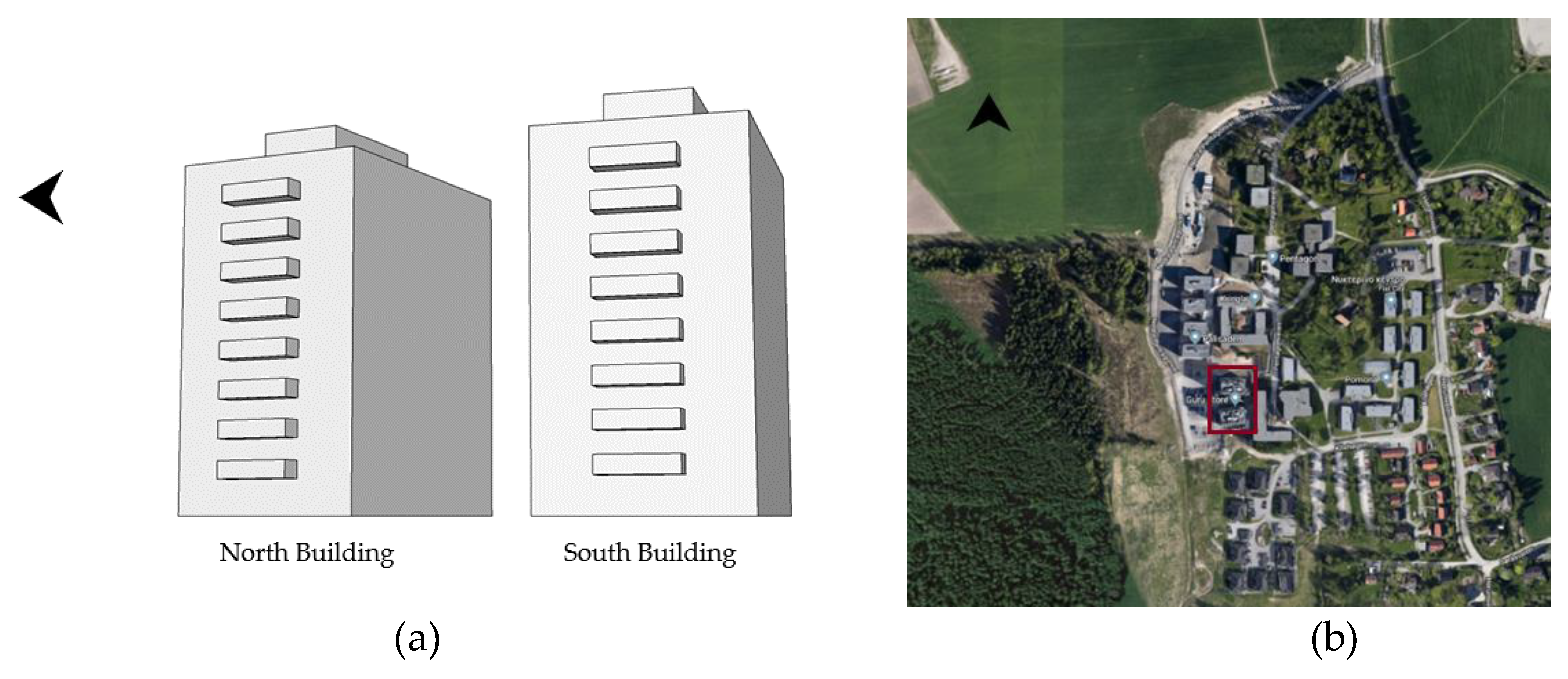
For the purpose of this study, full-scale measurements were performed in two twin medium-rise buildings. The measurements reveal the spatial variation of C_p values along the windward façades of the buildings. Furthermore, they capture the wind sheltering effect created in the case of a twin-building complex and, more specifically, the sheltering effect provided by one building to its twin. The use of fluctuating wind pressure coefficients for the calculation of air flow through an ideal crack is also investigated.

2. Methodology

2.1. Reference Buildings

For the purpose of this study, full-scale measurements were performed on the façades of a twin medium-rise building complex. The two identical buildings have the geometry of rectangular prism and they are oriented almost parallel to each other with an average distance of 12 m between them. The buildings’ long axes are running East–West. The buildings were erected in 2013 and they are built with cross laminated timber (CLT). They consist of eight floors each and their height is approximately 25 m (Figure 1a).

The twin buildings are situated in the rural town of Ås, Norway. The buildings are surrounded by some low-rise buildings (2–4 storeys) and they are located next to a forest area (Figure 1b).

2.2. Measurements

Twelve SDP1000 low-range differential pressure sensors for air—six at each building—were used during the measurements (Figure 2). The sensors have a measurement range of −5 to 125 Pa and they give high accuracy even below 10 Pa [24]. They also include a digital built-in temperature compensation circuit, thus rendering the measurements temperature independent. The pressure difference between the North façade (windward) and the reference pressure at the top of each of the twin buildings was measured simultaneously at both buildings.

All the reference pressure taps were placed at the same position at a height of approximately 2.5 m over the rooftop (Figure 2). The assumption that at this height the velocity vector has only a horizontal component is made. The pressure tap openings were placed parallel to the horizontal wind velocity vector. Therefore, the simplification that the pressure taps on the rooftops will only measure static pressure and not total pressure, since the velocity vector is parallel to the tap and will not increase the fluid’s speed, is made. The simplification that the pressure measured over the rooftop is the same as the static pressure at the undisturbed free stream at building height is also made.

Six pressure taps were placed in three different heights at the windward façades of the buildings. They were placed at the top, middle, and low parts of the building and in three different lateral positions: One close to each edge of the building and one in the middle of the building (Figure 2). The pressure taps had a diameter of 3 mm and they were placed in the middle of a square plate with an area of 0.01 m² in order to keep them perpendicular to the façade and also to reduce the turbulent flow around the tap nozzle (Figure 3). The pressure taps were connected with silicon tubes with a diameter of 3 mm to the differential pressure sensors according to the manufacturer’s suggestions. On the pressure side, the tube lengths varied from 15 m to 25 m, while on the reference position the tubes were 7 m.

Summarizing, it is considered that the measured differential pressure gives the difference between the pressure P_x at the tap’s position on the windward building façade and the static pressure P₀ at the undisturbed wind flow at building height.

The pressure sensors were placed at the rooftops of the twin buildings. The data acquisition system was recording the instantaneous pressure difference values with a frequency of 5 Hz. The full-scale measurements lasted approximately one week, during which the dominant wind direction was North (0°) (Figure 4). Therefore, wind pressure coefficients for only the North (0°) direction were calculated.

During the measurements, the wind speed and wind direction were monitored both by a weather station installed on the rooftop of one of the twin buildings and by the local meteorological station, which is situated approximately 600 m from the reference buildings. The weather station on the rooftop provided only 30-min averaged values, while the meteorological station gave 10-min averaged values for wind speed and direction. The most frequent weather data were considered more appropriate for the correct calculation of the wind pressure coefficients. Therefore, a correlation between the two stations were established and the 10-min averaged values were corrected according to the following process in order to account for the local wind speed variations on the rooftop of the reference buildings.

The meteorological station is situated in the middle of an open field and the wind data were measured at a height of 10 m over the ground. Using the logarithmic wind profile [25], the wind speed at the reference building height (h_ref = 25 m) was calculated based on the relevant roughness length (z₀ = 0.03 m) that corresponds to open agricultural land, similar to the meteorological field. The logarithmic wind profile is described by the following equation:

$$u_2=u_1\frac{\ln \left(\frac{h_2}{z_0}\right)}{\ln \left(\frac{h_1}{z_0}\right)},$$

(2)

where $u_1$ is the reference wind speed at height $h_1$, $u_2$ is the wind speed at height $h_2$, and $z_0$ is the roughness length depending on the land cover type.

Subsequently, the 30-min averaged wind speeds at a 25 m height over the meteorological field were calculated and compared with the corresponding 30-min averaged values given by the weather station at the rooftop of the twin buildings. A correction coefficient was determined for each one of 16 wind directions (N, NNE, NE, NEE, E, SEE, SE, SSE, S, SSW, SW, SWW, W, NWW, NW, NNW). The correction coefficients were applied to the 10-min averaged wind speeds from the local meteorological station at 25 m according to the wind direction. The corrected 10-min averaged data at 25 m over the meteorological field correspond to the 10-min averaged wind speeds at the reference building height and were used for the calculation of the C_p values based on Equation (1) (Figure 5). As a result, both freestream wind velocity and freestream pressure were theoretically measured at the same position over the rooftop of the reference buildings.

2.3. Monte Carlo Simulations

The measurements showed that the measured wind pressure coefficients were fluctuating significantly during the measuring period. For the purpose of this study, both the use of fluctuating wind pressure coefficients and the use of the measured mean C_p values for the calculation of air infiltration were evaluated.

Since the wind pressure coefficients were measured only on the windward sides of the reference buildings, the impact of the C_p values on air infiltration was evaluated qualitatively, assuming an ideal gap of area of 0.01 m². In this case, the air flow can be represented by an equivalent flow through a flat orifice plate [18]. The orifice flow is given by the following equation:

$$Q=C_{d}A\sqrt{\frac{2}{\rho }\Delta P},$$

(3)

where $Q$ is the air flow rate (m³/s), $C_d$ is the discharge coefficient (in this study taken as equal to 1), $\rho$ is the air density (kg/m³), $\Delta P$ is the pressure difference across the opening (Pa), and $A$ is the area of the opening (m²).

Combining the orifice equation and the defining equation for wind pressure coefficients, the air flow through the assumed ideal gap can be given by the following equation:

$$Q=A\cdot U_{wind}\cdot \sqrt{C_p}.$$

(4)

In order to evaluate the fluctuating C_p values with respect to air infiltration, the Monte Carlo method was employed [26,27,28,29]. Initially, the actual distribution of the measured wind pressure coefficients was determined and, after applying data fitting, it was found that the measured C_p values follow the logarithmic normal distribution [23]. The logarithmic normal distribution cannot include negative values, thus the measured negative wind pressure coefficients have been excluded. However, for all measuring positions, besides the Middle West, the amount of measured negative values is between 1% and 3%, which can be considered negligible. At the Middle West measuring position, the negative values make up 8% of the total measured wind pressure coefficients.

The wind velocities measured during the measuring period were used. Only wind directions within the angle range [−22.5°, 22.5°] that correspond to the North wind direction were selected. Similarly, it was found that the wind velocity distribution follows the logarithmic normal distribution (Figure 6). The Weibull distribution was also considered, but the logarithmic normal distribution captured better the frequency of the measured wind speeds (Figure 6). The log-normal distribution is generally considered a suitable distribution to describe the probability distribution of wind speed data [30,31,32,33].

The Monte Carlo simulations repeat random sampling from the two log-normal distributions of wind pressure coefficients and wind velocities, and subsequently calculate the resulting air flow (Figure 7a). In order to define the required number of iterations for the Monte Carlo simulations, 50,000 iterations were performed and the sample average was plotted against the number of iterations. The results indicated that the simulations reach convergence after approximately 7000 iterations. Consequently, 10,000 iterations were performed for the Monte Carlo simulations that calculated the air infiltration in each one of the six measuring positions.

Furthermore, Monte Carlo simulations were also performed in order to define the air infiltration through the ideal gap using constant time-averaged C_p value (Figure 7b). In that case, the Monte Carlo simulation was used in order to randomly select values from the log-normal distribution of the wind velocities. For this case also, the total number of iterations performed was 10,000.

Furthermore, the air flows were calculated using the measured wind pressure coefficient and corresponding measured wind speed at each time step, and the actual air flow distribution at each measuring position was defined (Figure 8a). The Monte Carlo simulation results for both cases—using fluctuating C_p values and mean C_p value—were evaluated against the actual air flow distributions that were calculated using the measured wind pressure coefficients and measured wind speeds at each time step.

During building energy simulations, the air changes are calculated using mean C_p values and hourly wind data from typical meteorological year (TMY) files. Therefore, an additional air flow through the ideal gap was calculated using the mean C_p values in combination with hourly-averaged wind speeds for the North wind direction (Figure 8b).

3. Results

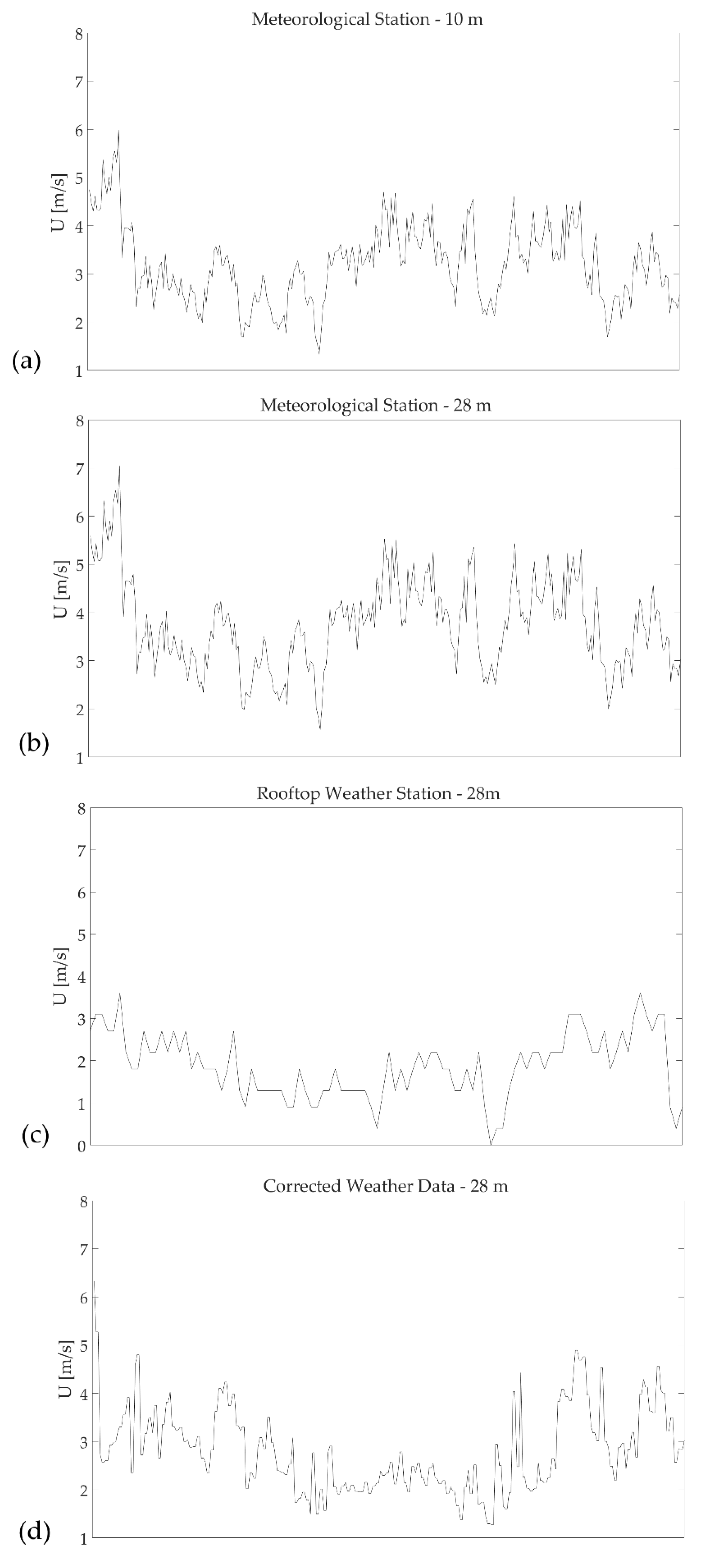
For the determination of the wind pressure coefficients on the North façades of the two reference buildings, only weather data that corresponded to North wind direction, and more specifically wind angles within the range of −22.5° to 22.5°, were used (Figure 4). The wind pressure coefficients were calculated from Equation (1), using the differential pressure provided by the sensors and the corrected wind velocity at the building height. The air density was also calculated using the pressure, temperature and humidity values provided by the weather station.

Initially, the fluctuating differential pressure data obtained during the pressure measurements were smoothed and the “noise” due to the length of the silicon tubing used was filtered out by the means of moving average [34].

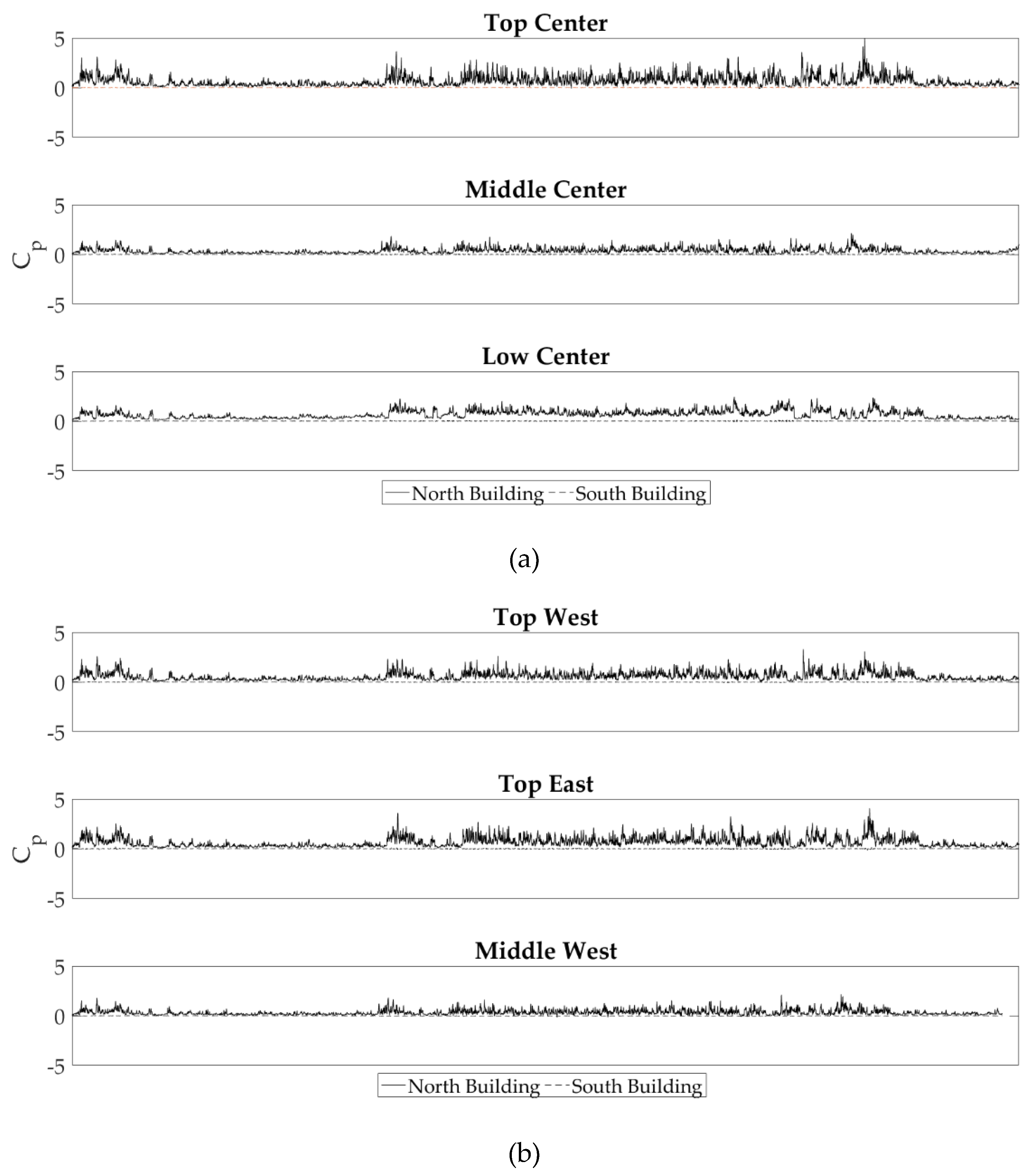
Figure 9 shows the measured wind pressure coefficients at the various measuring positions for both buildings. We remind that, during the measurements, the dominant wind direction was North (Figure 4). As it is expected, the North building, which is completely exposed to the impinging wind, presents high values of wind pressure coefficients on its windward façade. On the other hand, the South building that is protected by its twin from the incoming North wind develops no essential wind-induced pressure on its windward façade.

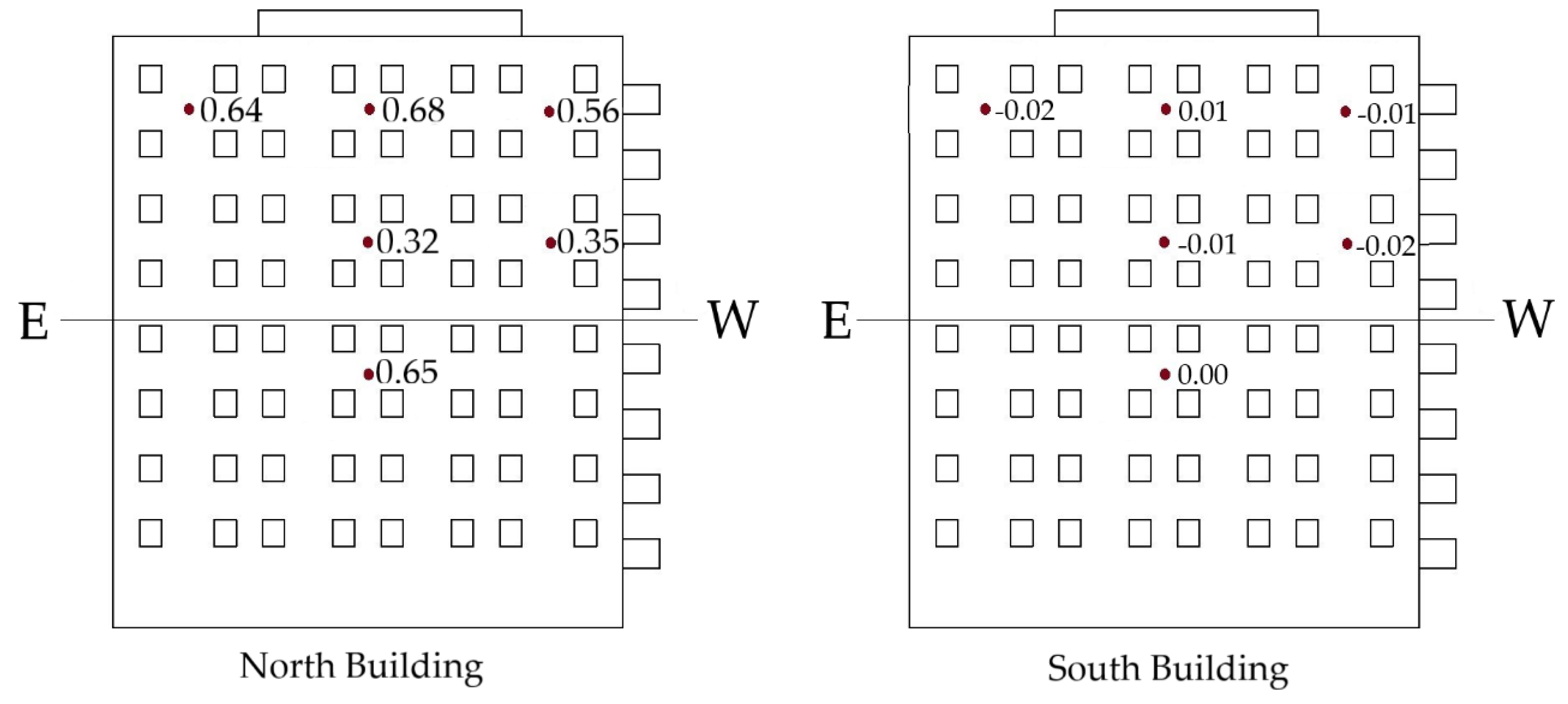
Figure 10 presents the mean measured wind pressure coefficients at the measuring positions on both twin buildings.

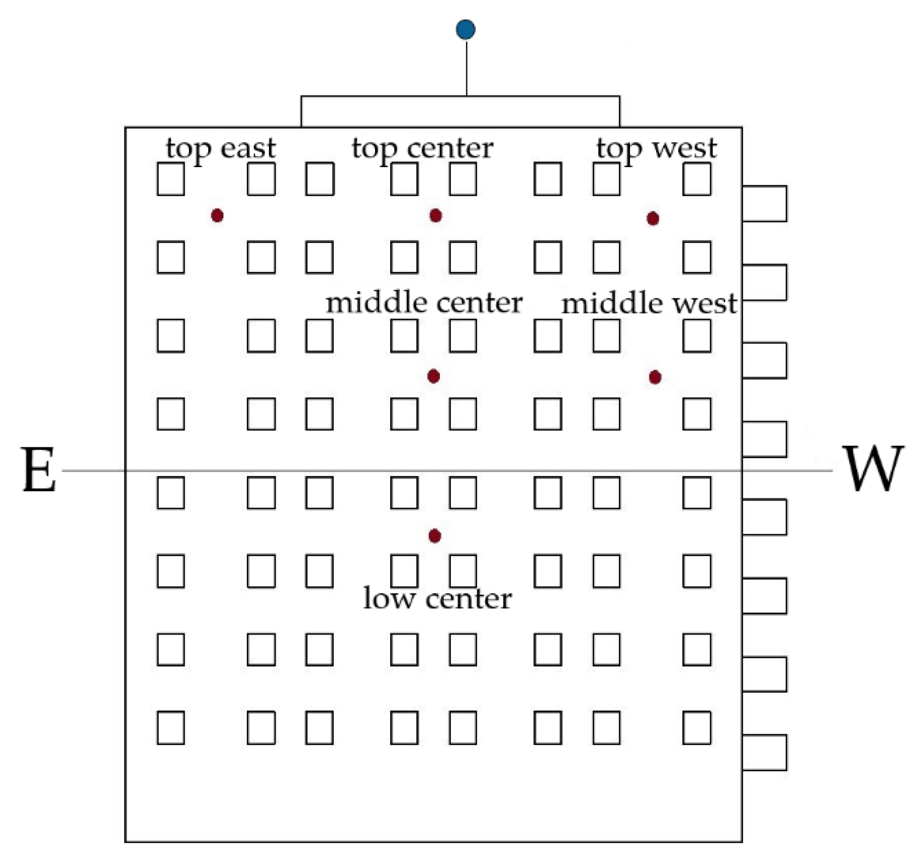
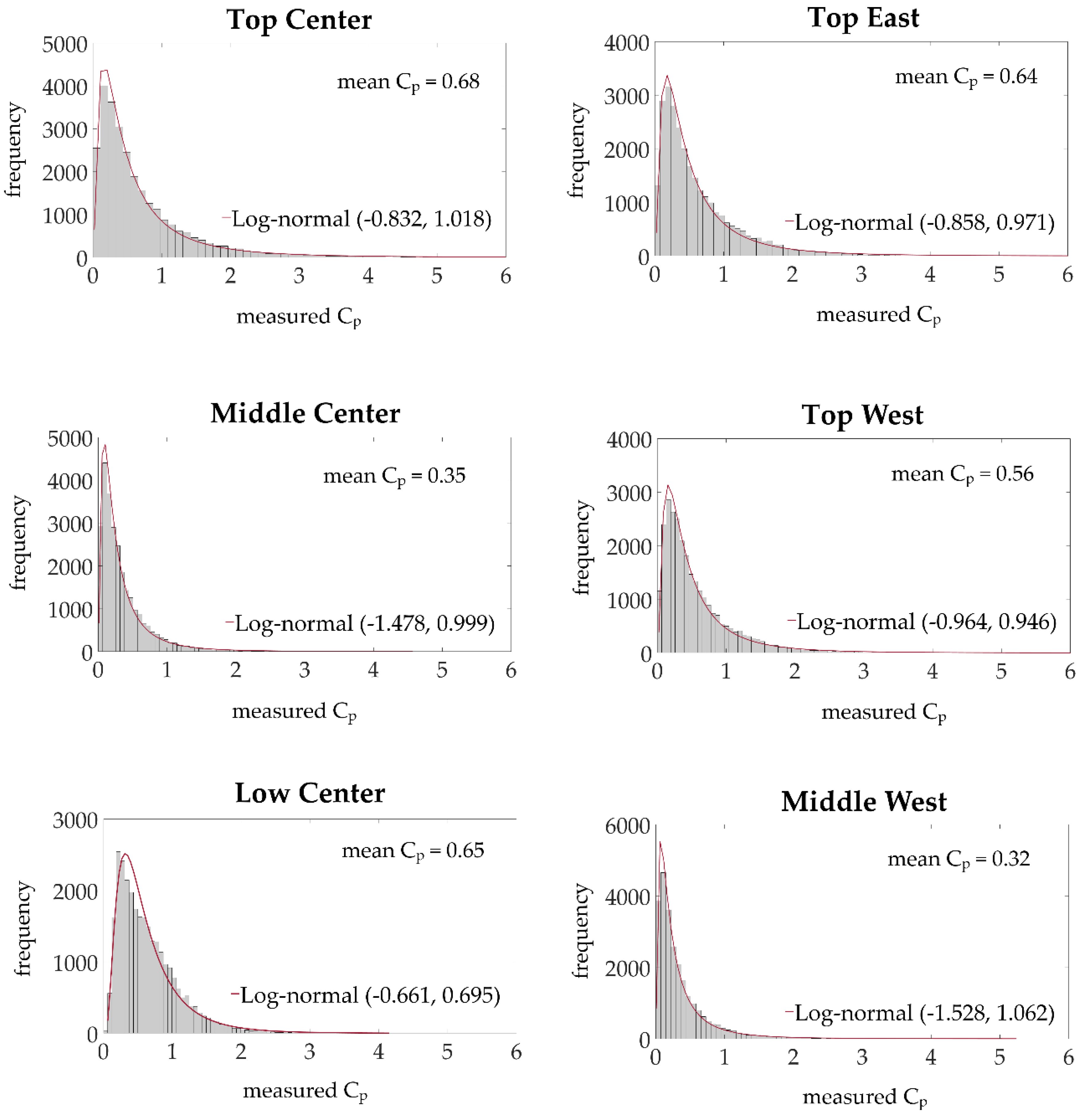
The wind pressure coefficients calculated for the highest part of the North building have relatively the highest values, as it would be expected. The top center part is the most susceptible to wind pressure with a measured C_p value of 0.68. Both positions close to the edges present lower pressurization compared to the center of the building envelope and their measured C_p values are 0.64 and 0.56 for the East and West positions, correspondingly. It is interesting that, although the edge measuring positions are symmetrical to the center, they do not have similarly lower measured wind pressure coefficients compared to the center. In contrast, the middle part presents no essential variation between the center and the edge and both measured wind pressure coefficients are approximately at 0.34. However, it is highly interesting that these middle positions are placed on the top half of the building but they deviate almost by half the measured values on the top part. More specifically, the middle measuring position is placed approximately 2/3 up the building, which is similar to the stagnation point position, where the wind-induced pressure is expected to be the highest. On the other hand, the mean measured C_p value on the low center position was calculated at 0.65. Consequently, and in contrast to what might be expected, i.e., the C_p values decreasing as the positions are moving lower across the vertical axis of the building, the measurements show that the highest wind pressure coefficients are measured both on the top and in the low measuring positions, while the lowest wind pressure coefficient is measured on the middle measuring position. This is probably the result of the surroundings’ morphology, as the neighboring buildings can provide wind shelter to the middle measuring zone and other neighboring buildings or obstacles can create an upwind flow that causes the increased wind-induced pressure on the lower measuring zone. However, since no wind or turbulence measurements were performed on site, it can only be assumed that the particular pressure variation pattern along the building façade is the result of the microclimatic effect.

As it can be seen in Figure 10, all six mean measured coefficients on the South building are practically zero. Slightly over zero, with a C_p value of 0.01, is the wind pressure coefficient of the top center measuring position. The measured C_p values on all edge positions are slightly below zero, between −0.01 and −0.02, probably due to the induced turbulence on the edges of the building. However, the measured C_p values on the two remaining center points (middle center and low center) of the South Building indicate that the turbulence developed in the passage between the twin buildings is negligible. The results show that for North wind, the South building is completely sheltered from the impinging wind by its twin North Building and no essential wind-induced pressurization is developed on its windward façade.

Figure 9 shows that the measured wind pressure coefficients fluctuate significantly during the whole measuring period for the windward façade of the exposed North building. Therefore, Monte Carlo simulations were performed in order to investigate the impact of fluctuating C_p values on the air infiltration calculation and to assess whether the use of the mean C_p values is sufficient. Since the measured wind pressure coefficients on the windward façade of the sheltered South building fluctuate slightly around 0.0, the Monte Carlo method was employed only for the windward façade of the exposed North building.

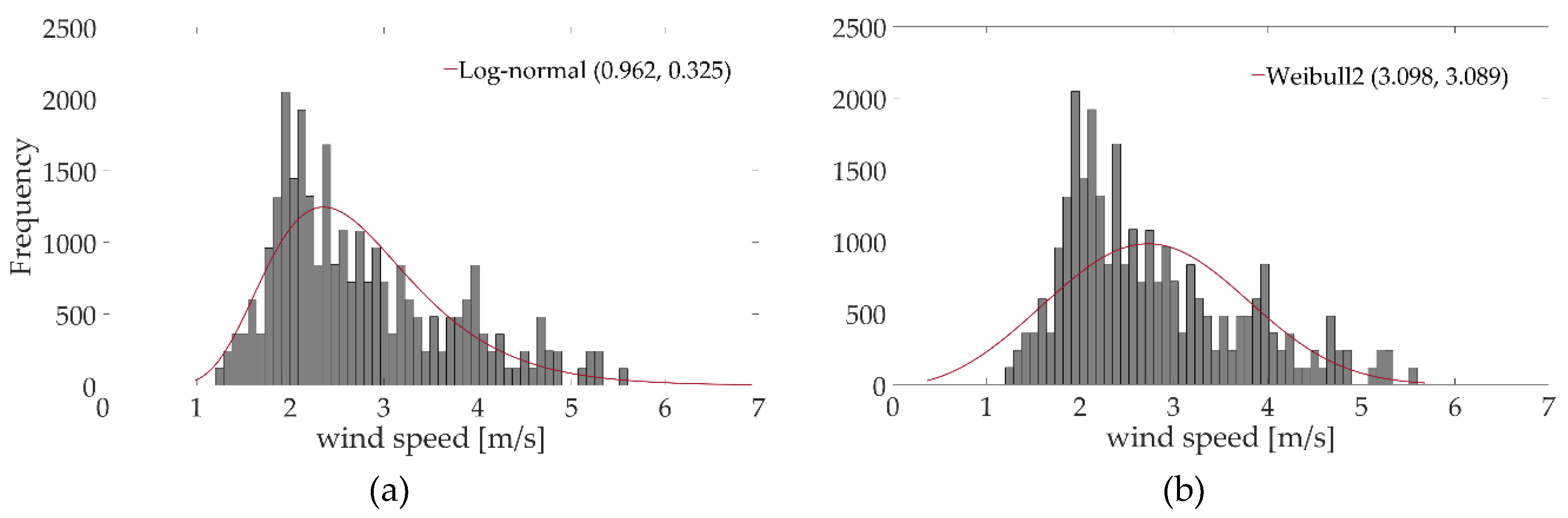
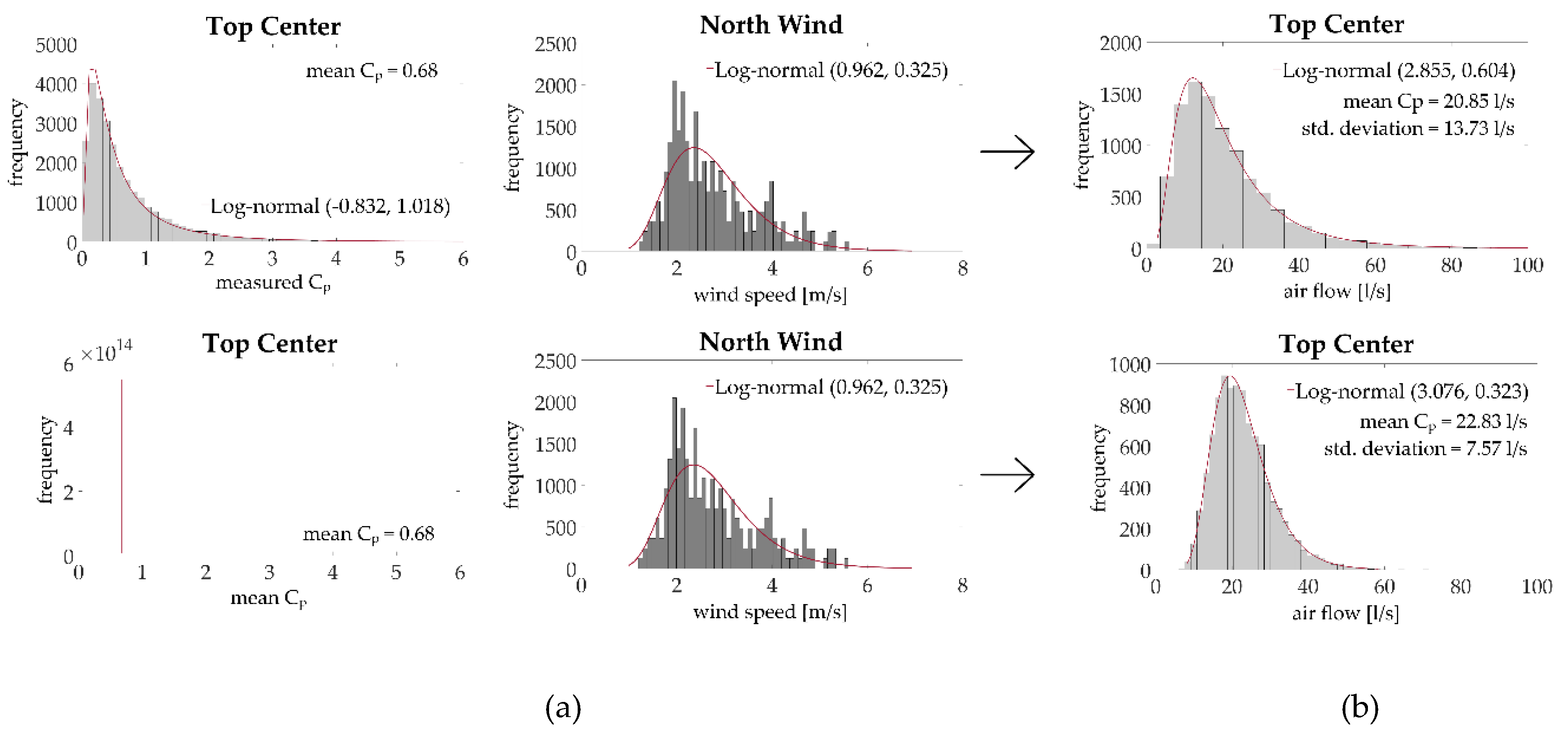
Figure 11 shows all the histogram distributions of the measured wind pressure coefficients on the windward façade of the exposed North building, along with their corresponding probability distribution functions. It is interesting that in all measuring positions, the wind pressure coefficient distribution follows the logarithmic normal probability function, however, the findings regarding the probabilistic nature of the measured wind pressure coefficients are in accordance with previous study findings [23]. The probability distribution functions of the measured wind pressure coefficients were used in combination with the probability distribution function of wind speeds for the North direction by means of the Monte Carlo simulation, as described in Section 2.3.

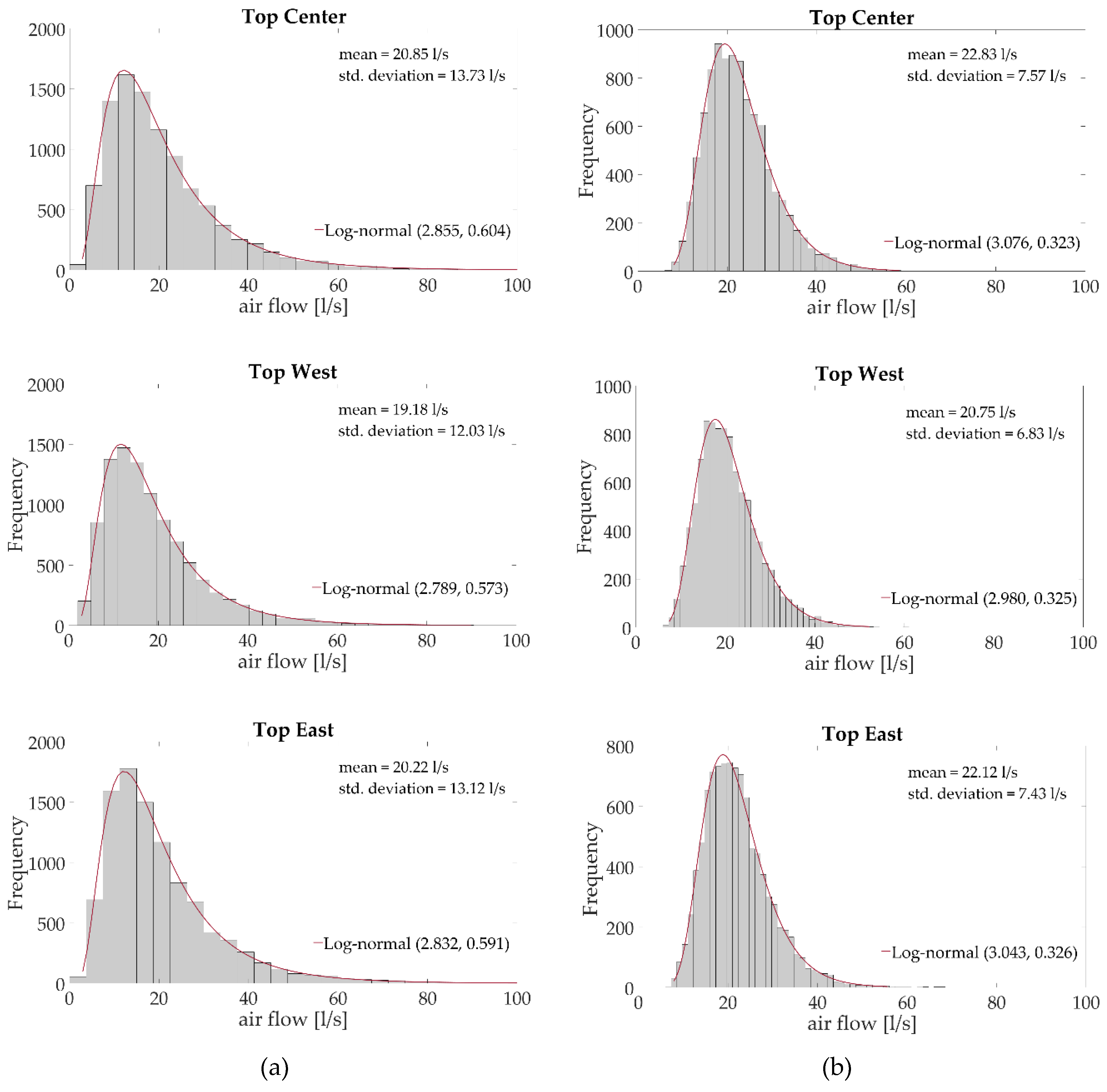
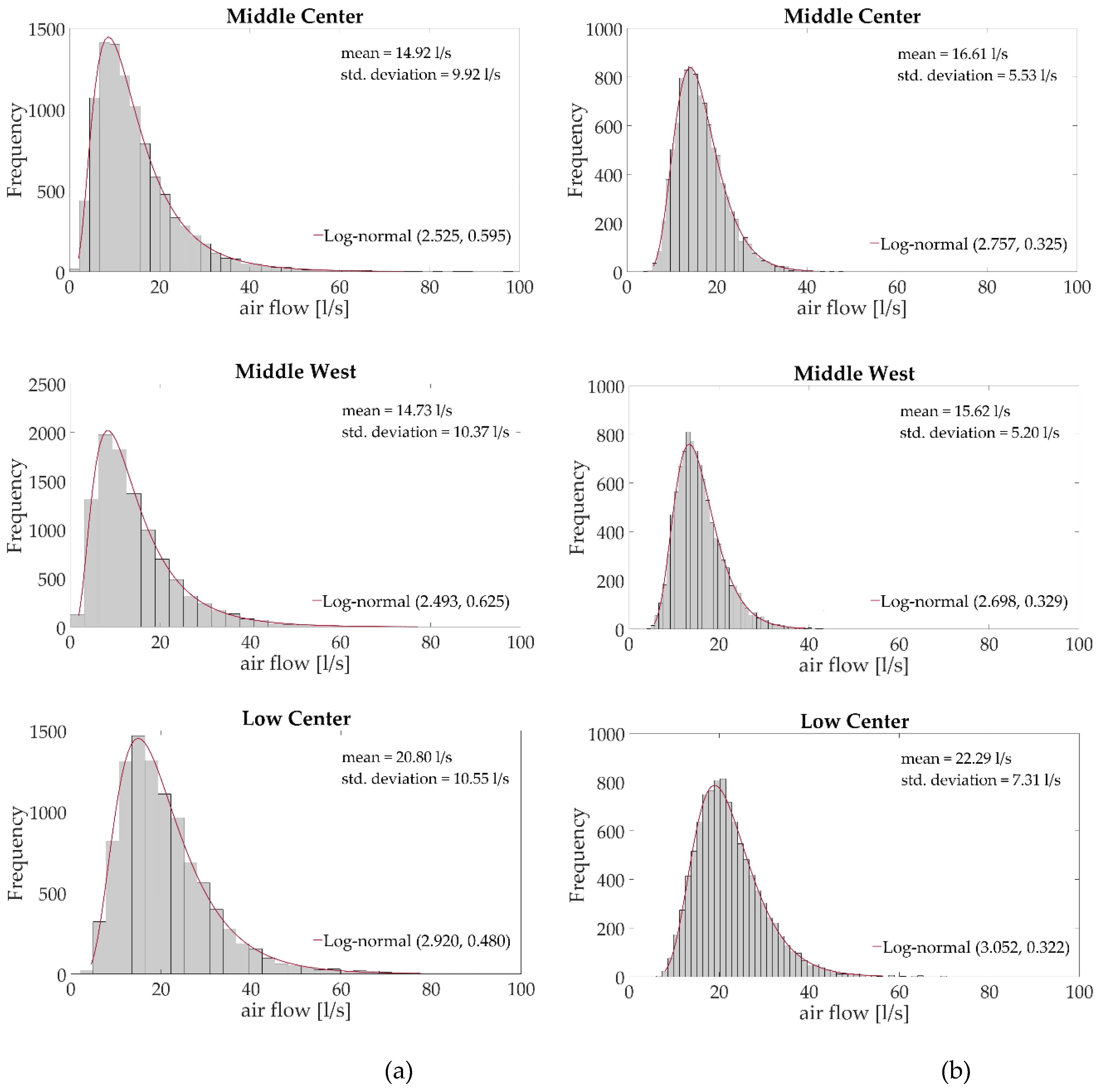
Figure 12 and Figure 13 show the probability distributions of the air flows, calculated both using the probability distribution of measured C_p values and the constant mean C_p value. For both cases, all probability distributions are constructed at a confidence level of 95%, and they all follow the logarithmic normal distribution function. In all measuring positions, the log-normal distribution functions derived from fluctuating C_p values have a slightly higher parameter σ and a lower parameter µ, which means that the corresponding density distribution is slightly more shifted toward the left side of the x-axis, compared to the density distribution of air flow derived from the constant mean C_p value. Although the resulting air flow probability distribution function (pdf) using mean C_p value will be closer to the peak value of the actual air flow rate, the air flow pdf resulting using fluctuating C_p values will always capture better the overall distribution of the air flows and produce a sample mean closer to the actual air flow mean (Figure 14).

Furthermore, for all measuring positions, the sample mean calculated using mean C_p values is always higher than the corresponding sample mean using fluctuating C_p values, while the sample standard deviation using mean C_p value is always lower than the corresponding one using fluctuating C_p values. The sample means differ between 4% and 10%, while the standard deviation differences vary from 1% to 30%. Overall, the results suggest that the use of mean C_p values tends to calculate larger air flows by approximately 7% in comparison to the mean air flow results given by using fluctuating C_p values. In both cases, the calculated air flow distributions follow similar logarithmic normal distribution.

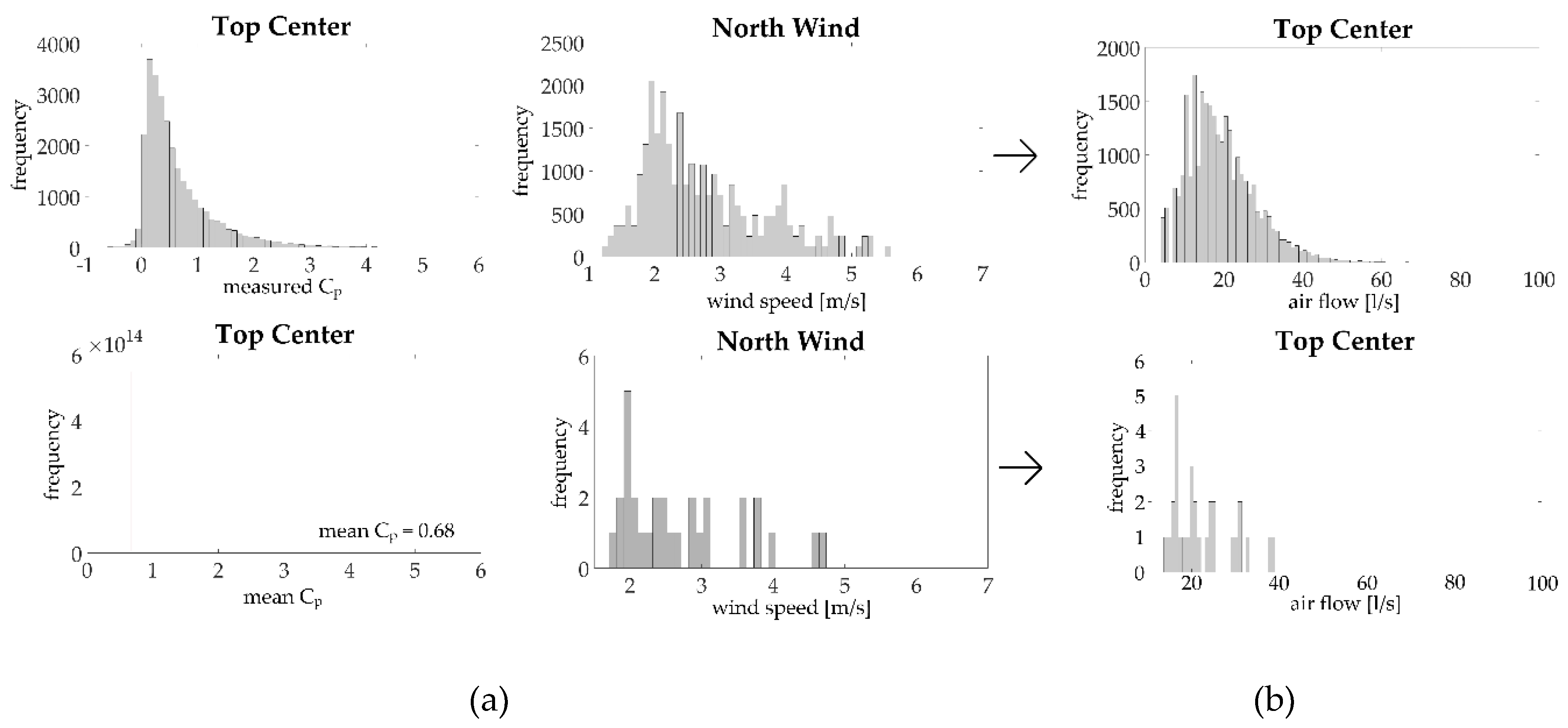
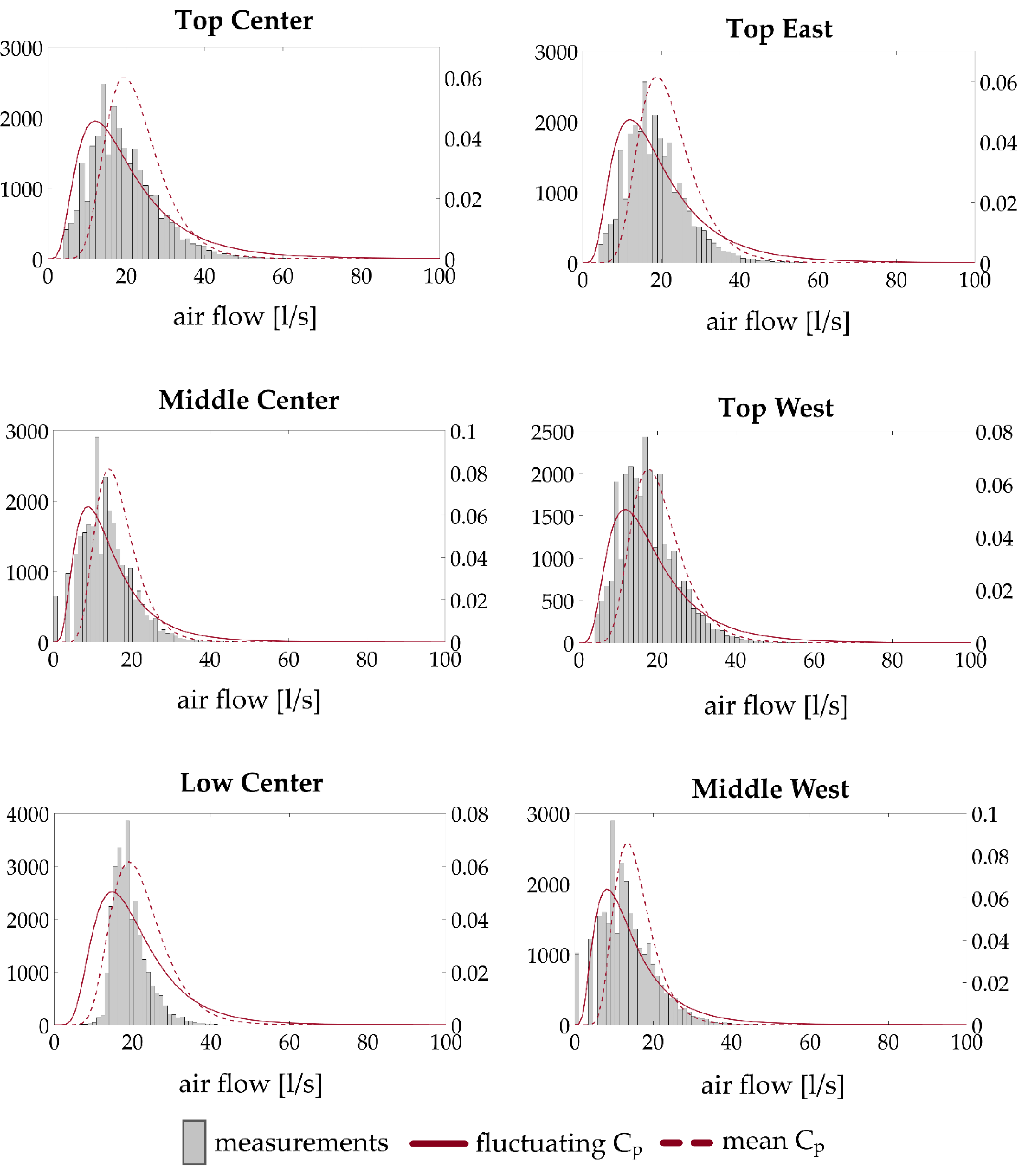
The Monte Carlo results using both fluctuating and mean C_p values are also compared with the actual air flow distributions that are calculated using the measured wind pressure coefficients and measured wind speeds at each time step (Figure 14). Figure 14 shows that the statistical methods slightly overestimate the air flow regardless of the input considered for the C_p values (probability distribution of fluctuating C_p or mean C_p), but overall, both resulting distributions seem to fit rather sufficiently with the measured data. During the Monte Carlo simulations, random values of the two distributions (wind pressure coefficient and wind speed) are combined in order to calculate the air flow. On the other hand, during the calculation of the actual air flow distribution, the measured wind pressure coefficient is combined with the corresponding measured wind speed at each time step in order to calculate the air flow and therefore, it is easier to capture the wind gust effect.

In all measuring positions, the use of the fluctuating C_p value on Monte Carlo simulations produces results closer to the actual air flow distribution. For fluctuating C_p values, the sample-average air flows deviate by less than 10% from the mean air flow calculated using the measured data, while the corresponding sample mean using mean C_p value deviates by 17–23% from the measured mean (

Table 1. Mean air flow using measured data and sample average air flow calculated through the Monte Carlo simulations.

Method	Top East	Top Center	Top West	Middle Center	Middle West	Low Center	RMSE
Measured	18.59 L/s	19.27 L/s	17.68 L/s	13.52 L/s	13.32 L/s	19.29 L/s	-
Fluctuating Cp	20.22 L/s	20.85 L/s	19.18 L/s	14.92 L/s	14.73 L/s	20.80 L/s	1.51 L/s
Mean Cp	22.12 L/s	22.83 L/s	20.75 L/s	16.61 L/s	15.62 L/s	22.29 L/s	3.12 L/s
Mean Cp + Uhourly	20.37 L/s	22.44 L/s	20.37 L/s	16.10 L/s	15.40 L/s	21.94 L/s	2.53 L/s

). Overall, the use of fluctuating C_p values in combination with wind speed probability distribution function gives a root mean square error (RMSE) of 1.51 L/s, while the use of mean C_p value in combination with wind speed pdf gives an almost double corresponding RMSE of 3.12 L/s.

Furthermore, for every measuring position, the air flow through the ideal gap was calculated using the mean C_p value in combination with hourly-averaged wind speeds. The results show that this conventional way of calculating air flows deviates approximately 10–20% from the actual air flows and produces a RMSE of 2.53 L/s. It is worth noting that, although the conventional method is the most simplified method used to calculate air flows, it produces better results with lower RMSE compared to the use of mean C_p in combination with wind speed pdf.

Both the calculated air flow probability distributions and the calculated air flow distribution highlight the significance of area-specific wind pressure coefficients instead of surface-averaged wind pressure coefficients for the air infiltration calculations [9,11]. The air flow differs substantially between measuring positions accordingly to the measured wind pressure coefficients. For example, the mean calculated air flow using measured data for the top center measuring position is calculated at 20.85 L/s, while the corresponding mean air flow for the middle center position is calculated at 14.92 L/s, signifying a difference of approximately 28%. The spatial difference on air flow due to the spatial variations of wind pressure coefficients can be seen through the statistical method, regardless of the input—probability distribution function or mean C_p value. Although the sample-average air flow values using the probability distribution function and the mean C_p value on Monte Carlo simulations are higher than the measured mean air flows, they still manage to capture the same deviation of 28% between the calculated air flow at the top center and at the middle center position. Similarly, the spatial variation is also captured by the conventional calculation method. As a result, the determination of wind pressure coefficients with spatial resolution along the façades of medium- and large-scale buildings can significantly improve the calculation process of air changes.

4. Discussion

Full-scale measurements for the determination of wind pressure coefficients have been performed in a twin medium-rise building complex. Conventionally, full-scale measurements have been performed in low-rise buildings with simple geometries for the determination of characteristic wind loads and the validation of wind-tunnel tests. In this study, the on-site pressure measurements performed highlight the spatial variation of the wind pressure coefficients along the windward façade of a building complex. The case of the building complex examined indicates that the surroundings can have a significant impact on the wind-induced pressure variations along the building façades and can lead to very building-specific spatial wind-induced pressure variations and consequently to building-specific wind pressure coefficients. Although full-scale measurements are difficult to perform for each individual case, CFD simulations can be employed in order to determine building-specific wind pressure coefficients with respect to the microclimate. In addition, in cases of twin-building complexes, the microclimate formed by the two buildings has a clear effect on the wind-induced pressure coefficients. The full-scale measurements show that for specific wind directions, one building can provide substantial wind shelter to its twin. This fact, in combination with local weather patterns (for example, in a town with a specific annual dominant wind direction), can lead to considerably reduced wind loads acting on one of the buildings throughout the whole year.

Furthermore, studies describe the uncertainties introduced in the air flow rate calculations due to the use of surface-averaged wind pressure coefficients. The on-site measurements performed within the context of this study strengthen the aforementioned argument and show that the wind pressure coefficients of the windward façade of a medium-scale building can vary in a significantly spatial way along the façade. Furthermore, the air flow calculations performed show that positions with significant differences in the measured wind pressure coefficients present equally significant differences of their corresponding calculated air flow rates. Therefore, the determination of local wind pressure coefficients with high resolution along the building façades seems to be a suitable method that can increase the air flow rate calculation accuracy.

Studies have also described how the wind gustiness effect has a great impact on air infiltration. In addition, studies have also described the probabilistic nature of wind pressure coefficients. The Monte Carlo method seems a promising solution that can combine the probability distribution functions, which describe the fluctuating nature of wind pressure coefficients, and the probability distribution function of wind velocity, which can account for the occurring wind gusts. The use of mean C_p values in combination with the pdf of wind speed, as well as the conventional method of calculating air flow rates (mean C_p value in combination with hourly-averaged wind speeds), have also been evaluated. The results show that use of probability distribution functions for both C_p values and wind speeds by means of the Monte Carlo method produce the most accurate results regarding the calculated air flow rates.

5. Conclusions

The full-scale measurements performed for the purpose of this study showed that wind pressure coefficients vary significantly along the façade of medium-rise buildings, with the measured C_p values varying by even 50% between two height zones. Furthermore, the measurements showed that, in cases of twin-building complexes, under certain wind conditions, one building can provide substantial shelter to its twin. Overall, the results give an indication for the importance of the surroundings on the determination of wind-induced pressurization of buildings.

Furthermore, the results showed that positions with significant differences in their local measured wind pressure coefficients present similar differences in the corresponding calculated air flow rates, thus highlighting the importance of including local C_p values and not surface-averaged for the calculation of air infiltration. Based on the measured data, the variation of wind pressure coefficients along the building façade can lead to up to 28% difference of air flow rates among the various positions on the building façade.

Last but not least, the use of probability distribution functions of C_p values, instead of mean (time-averaged) C_p values, in combination with the probability distribution function of wind speeds, can increase the accuracy of the air flow rate calculation. The results indicate that the use of probabilistic C_p values can increase the accuracy of air flow rate by 40% compared to the conventional method, which employs mean C_p values in combination with hourly-averaged wind speeds. As a result, the suggested method has the potential to improve the overall prediction of the building energy demands.