The Spatial and Temporal Variability of the Indoor Environmental Quality during Three Simulated Office Studies at a Living Lab

Abstract

The living lab approach to building science research provides the ability to accurately monitor occupants and their environment and use the resulting data to evaluate the impact that various components of the built environment have on human comfort, health, and well-being. A hypothesized benefit of the living lab approach is the ability to simulate the real indoor environment in an experimentally controlled setting over relatively long periods of time, overcoming a significant hurdle encountered in many chamber-type experimental designs that rarely reflect typical indoor environments. Here, we present indoor environmental quality measurements from a network of sensors as well as building system design and operational data demonstrating the ability of a living lab to realistically simulate a wide range of environmental conditions in an office setting by varying air temperature, lighting, façade control, and sound masking in a series of three human subject experiments. The temporal variability of thermal and lighting conditions was assessed on an hourly basis and demonstrated the significant impact of façade design and control on desk-level measurements of both factors. Additional factors, such as desk layout and building system design (e.g., luminaires, speaker system), also contributed significantly to spatial variability in air temperature, lighting, and sound masking exposures, and this variability was reduced in latter experiments by optimizing desk layout and building system design. While ecologically valid experimental conditions are possible with a living lab, a compromise between realism and consistency in participant experience must often be found by, for example, using an atypical desk layout to reduce spatial variability in natural light exposure. Based on the experiences from these three studies, experimental design and environmental monitoring considerations for future office-based living lab experiments are explored.

1. Introduction

Buildings are the habitat of the modern human, as we spend about 90% of our lives in homes, offices, schools, and vehicles [1]. The built environment directly impacts human health and well-being, making building design and operation crucial for managing and improving public health [2,3,4]. Human outcomes frequently identified as being impacted by the built environment include comfort (e.g., thermal [5] and acoustic comfort [6,7]), performance [8,9], sleep [10], stress [11,12], pollutant exposure [13], and a wide range of other health and behavioral outcomes, such as musculoskeletal pain [14], posture [15], pathogen transmission [16,17,18], allergen exposure [19,20], workplace collaboration [21], and privacy [22,23].

1.1. Experimental Design in Building Science

In the building sciences, including the areas of indoor air quality [13,19,24,25,26], dampness and mold [27], thermal comfort [5,28,29,30,31,32], acoustics [6,33], green buildings [4,34,35], lighting [36,37], and indoor environmental quality (IEQ) [9,38,39,40,41,42,43,44,45,46,47,48], chamber and field studies are the predominant experimental approaches for conducting human subject research relating measures of physical conditions to human outcomes. Typically, chambers are the dimensions of a small to medium-sized office and are equipped with building systems (e.g., ventilation system, lighting, sound masking) capable of maintaining stable experimental conditions. Exposure periods are on the order of hours to days, allowing measurements of short-term outcomes, such as comfort, with cohort sizes of tens to hundreds. The Institute for Environmental Research at Kansas State University and the International Centre for Indoor Environment and Energy at the Technical University of Denmark are examples of research chambers used, for example, to test the thermal interaction of people and their surroundings. Field studies occur in real buildings and can be conducted over both short (days to weeks) and long periods (months to years) in ecologically valid settings. Cohort sizes in field studies are comparable to those found in chamber-type studies, though in field studies, there is a reduced ability to control the environment as well as limitations in measuring participant experiences and exposures. Such uncertainty reduces the power of statistical models to attribute human outcomes to building interventions and environmental exposures.

Advances in mobile computing and ubiquitous sensing provide building science researchers the tools to extend chamber and field study-type approaches to be continuous, longer-term, and better controlled in “living lab”-type investigations. Within the scope of building science, we describe the living lab approach as one that simulates realistic environments in a well-controlled manner for the purpose of measuring the human impacts of building-related interventions, often using networks of environmental sensors, physiological measurements, and/or surveys. It is hypothesized that more accurate assessments of human–building interactions can be evaluated with the living lab paradigm, as behavior and health response data can be correlated directly with interventions, environmental exposures, or other characteristics of the built environment while maintaining people’s natural behaviors and interactions with their surroundings. While chamber-like experimental designs are possible to pursue with a living lab facility, living labs are uniquely suited to be used in crossover studies of outcomes that require longer monitoring periods for accurately measuring changes in outcomes, such as sleep quality and stress. Due to increased experimental complexity and study length relative to chamber and field studies, as well as space constraints, living labs may utilize smaller cohort sizes, and multiple cohorts may be required to measure statistically significant effects.

The living lab paradigm has origins in smart-building innovation and ubiquitous computing, with early examples being the Aware Home and the Intelligent Workplace at Carnegie Mellon [49,50], and a recent example being SenseLab [51]. In the last decade, living labs have been used to evaluate technology adoption [52], test healthcare delivery methods [53], and evaluate energy consumption behaviors [54,55]. Applied as a scientific research methodology, living labs are useful for observing long-term human–building interactions in ecologically valid settings [56]. While living labs have not been broadly adopted in the building sciences, recent field and chamber investigations successfully applied aspects of the approach, such as extensive environmental sensor networks, novel behavioral measurements, and/or wearable devices, to measure human outcomes in realistic or semirealistic settings. Examples include a chamber study evaluating the impact of air quality on cognitive performance [57]; a classroom study on personal fan use, thermal comfort, and cognitive performance [58]; an office study evaluating sound masking approaches and cognitive function [59]; a large-scale office study identifying workplace interactions from wearable and stationary sensors [60]; and an evaluation of office layout and its impact on collaboration [21].

1.2. Indoor Environmental Quality

The IEQ of the built environment describes the combination of environmental conditions to which building occupants are exposed and includes but is not limited to thermal conditions (e.g., air temperature, radiant temperature, humidity, and air flow), lighting conditions (e.g., illuminance, correlated color temperature (CCT), uniformity, glare, daylighting), air quality conditions and ventilation (e.g., odors, air pollutant and bioeffluent concentrations), acoustic conditions (e.g., noise level, reverb), aspects of exterior and interior design (e.g., desk layout, ergonomics, and privacy), and building policies (e.g., smoking bans and security) [9]. Environmental sensors are capable of real-time monitoring of many dimensions of IEQ, but cost and sensor quality/availability are limiting factors for continuously quantifying spatial variability in some aspects of the environment, such as radiant temperature, air velocity, and glare. Air quality monitoring using low-cost sensors has proven particularly difficult, especially for reactive species (e.g., ozone) and particulate matter due to issues with long-term sensor stability, ability to accurately calibrate sensors, and the impact of confounding by humidity or other gas-phase species [61,62,63]. Other environmental metrics are important to human-related outcomes yet are not adequately measured by modern sensor technologies, such as speech content and occupant activities. Increasing prevalence of real-time data analysis techniques and algorithm development may provide solutions to overcoming these gaps, and recent studies demonstrate a high level of accuracy for predicting some occupant activities based on environmental data (e.g., window opening, showering, cooking) [64,65].

It is generally hypothesized that by improving overall IEQ, human health and well-being are also improved by limiting adverse environmental exposures and experiences [38,45,66]. Designing buildings capable of providing high-quality IEQ across all environmental factors can prove challenging, as many aspects of IEQ are physically interrelated [67]. For example, a high flow rate ventilation system with MERV13 and activated carbon filtration may provide good air quality but can also lead to increased noise levels due to fan and duct noise as well as degraded thermal comfort due to increased air velocities near supply diffusers. Windows must be designed such that they provide access to daylight and view, aspects of IEQ occupants rate as highly important, while limiting glare and their impact on thermal comfort due to radiative heat transfer and draft.

While prior studies extensively characterized the physical interactions between factors of IEQ, there are still gaps in understanding how such factors interact to influence human perceptions of the indoor environment [41]. For example, reductions in perceived air quality were detected when participants experienced poor thermal and daylighting conditions in a living lab [56]. Thermal comfort is a classic example where combinations of environmental (air/radiant temperature, air velocity, humidity) and human characteristics (metabolic rate, clothing) combine to affect people’s perception of the thermal environment [68]. Lack of characterization of these interactions is a limitation in some prior investigations, especially from assessments of human responses to a single IEQ factor, as they tend to contain an incomplete description of environmental conditions and interior design of the buildings and chambers in which the research was conducted, limiting the confidence with which findings can be applied in practice. With the living lab approach, the ability to accurately simulate and characterize the physical interactions that occur in buildings is expected to improve the ability to measure the complex relationships between occupant behavior, health, and IEQ.

Here, we present an assessment of the experimental design, interior design, IEQ, and building system operation and control from three office-based living lab studies during which air temperature, natural and electric lighting, and sound masking were varied between experimental conditions, the human outcomes of which are reported elsewhere [56,69,70]. We aim to address the questions: Can a living lab facility accurately simulate a typical office environment and IEQ conditions for the purpose of conducting human subject research? How do experimental designs aiming to evaluate one IEQ factor (e.g., daylighting) impact other factors (e.g., air temperature) in realistic scenarios, and how might these concomitant effects impact the ability to discern human outcomes? Data collected from the three experiments were used to characterize the spatial and temporal variability in IEQ conditions of the office environment simulated in each study. Results demonstrated the living lab can simulate an office environment within ranges typically found in real buildings, although careful attention must be given to building system design and operation, desk layout, and façade control such that experimental conditions are consistent across participants while simulating the natural temporal variability in environmental conditions found in real offices.

2. Methods

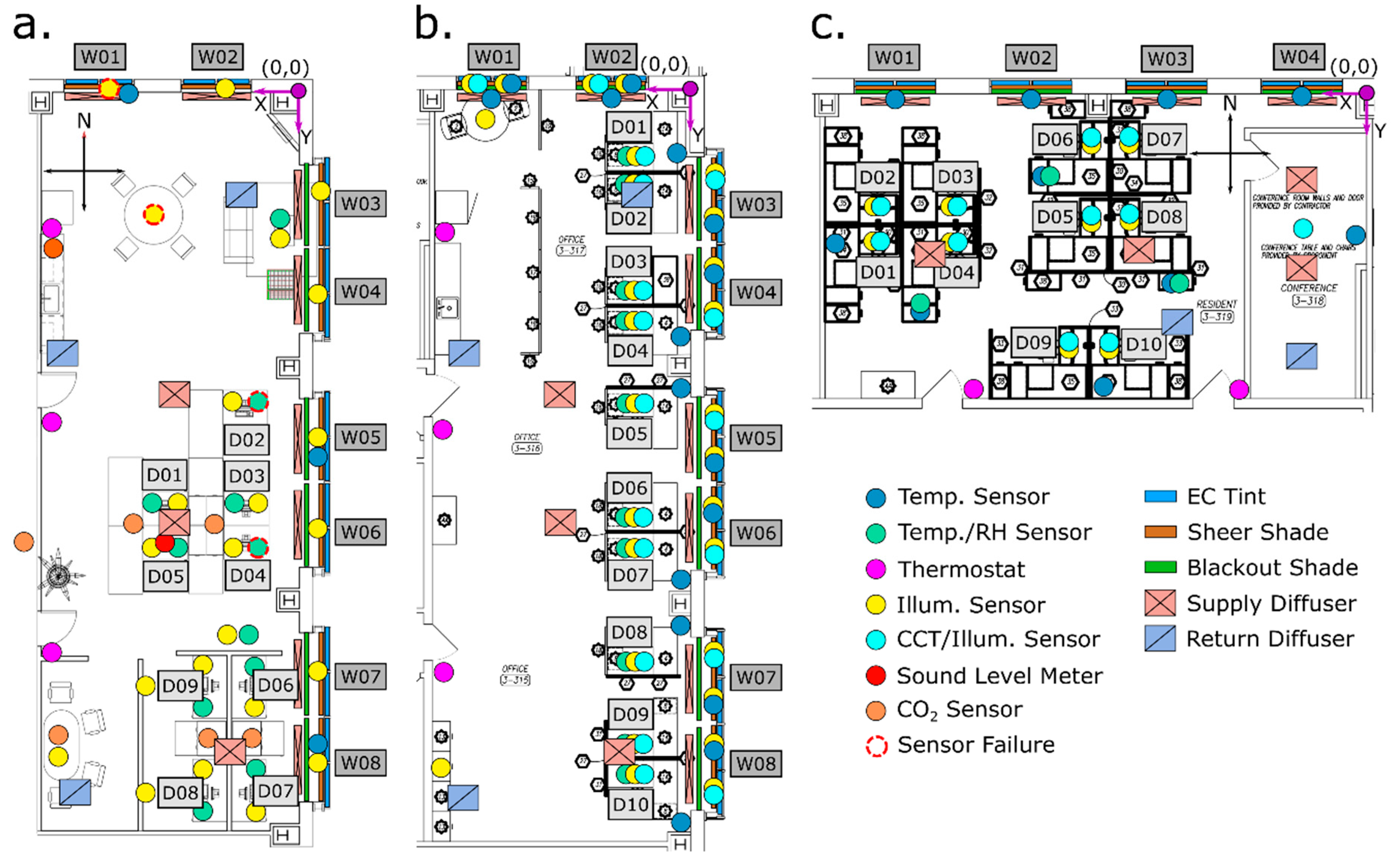
2.1. Facility Description

Experiments were conducted at the Well Living Lab, a living lab research facility located on the third floor of a downtown business building in Rochester, Minnesota, USA designed to conduct human-subject research utilizing six reconfigurable experimental rooms, or modules. Design elements such as raised floors, in-ceiling supports for device mounting, demountable walls, flexible power cable and water pipe routing, flexible air ducting, and a patchable communications network allow the modules to be extensively remodeled to simulate various real-world building interiors, allowing the facility to accommodate a wide range of experimental designs and/or cohort requirements. In the office setting, amenities provided to participants include a conference area for private discussions and meetings, a break area for meals and relaxation, printers and fax machines, secure network services, phone services, secure facility access, ergonomic chairs, and manually adjusted sit–stand desks that can be locked at a specific height if required by the experimental design. A participant was assigned to each desk (D##) in Figure 1, except D05 in the multi-IEQ study (Figure 1a), which was left unoccupied.

All building systems at the facility are controlled and monitored via a central building management system (BMS), including the heaving, ventilation, and air conditioning (HVAC), lighting, motorized roller shades (blackout and mesh), electrochromic window tinting, and audio systems. Two air handling units (AHU) provide mechanical ventilation to three modules each, with each module containing a variable air volume (VAV) damper with reheat for module-level control of supply flow rate and air temperature. Figure 1 describes locations of ventilation diffusers, shading, and tinting systems for each study.

All windows are equipped with electrochromic tinting (View, Inc.), capable of tinting to four distinct levels with visible light transmittances ranging from 58% (level 1) to 1% (level 4), and a pair of roller shades, one semitransparent mesh shade (E Screen—THEIA^TM, White/Pearl, Lutron Electronics Co., Inc., Coopersburg, PA, USA), and one blackout shade (Mermet Blackout-White, Lutron Electronics Co., Inc., Coopersburg, PA, USA). Lighting designs for each experiment are included in Figure S1 of the Supplemental Information. One experiment utilized the overhead speaker system to introduce either background office sounds or white noise into the office environment. Additional details of the audio system are included in Jamrozik et al., 2018 and Figure S2 depicts the spatial placement of in-ceiling speakers (CMS 403DCe Speakers, Tannoy Ltd., Coatbridge, UK). HVAC data reported below include thermostat temperatures (installation height of 1.35 m), AHU flow rates, VAV flow rates per module, and AHU return air relative humidity (RH). Window shade height and tint level state data are included in analyses of the impact of building system operation on lighting and temperature.

2.2. Experimental Design

2.2.1. Overview

Table 1. Experimental design summary of three office-based living lab experiments.

Condition Name	Week No.	EC Glass (Tint No., Control?)	Mesh Shades (Black-Out Shades)	Desk-Surface Electric Light Illuminance (lx)	Lighting CCT (K)	Temp (°C)	RH (%)	Sound Masking
Multi-IEQ Study (5/31/2016-9/30/2016)
Near-Optimal (Baseline)	1, 5, 10, 14	Level 1 (None)	Open, Operable (Open)	-	3500	21.7	40	None
Optimal	2, 6, 9, 11, 15, 18	Intelligence (None)	Open, Operable (Open)	-	4200	21.7	40	None
Sub-Optimal 1	3, 12	Level 4 (None)	Closed, Inoperable (Closed)	-	2700	19.4	40	White Noise, Low Volume
Mixed 1	4, 13	Level 1 (None)	Open, Operable (Open)	-	2700	23.9	40	Office Sounds 1
Sub-Optimal 2	7, 16	Level 4 (None)	Closed, Inoperable (Closed)	-	6500	19.4	40	White Noise, High Volume
Mixed 2	8, 17	Intelligence (None)	Open, Operable (Open)	-	6500	23.9	40	Office Sounds 2
Daylighting Study (6/19/2017-9/8/2017)
No View (Baseline)	1, 2, 9, 10	Level 4 (None)	Closed, Inoperable (Closed)	300	4000	23.9	40	None
Mesh Shades	5, 6, 11, 12	Level 2 (None)	Open, Operable (Open)	300	4000	23.9	40	None
Dynamic Tint	3, 4, 7, 8	Intelligence (App override)	Open, Inoperable (Open)	300	4000	23.9	40	None
Electric Lighting Study (7/10/2017-9/8/2017)
Fluorescent (Baseline)	1-4	Level 4 (None)	Closed, Inoperable (Closed)	250	3300	22.8	40	None
LED	5-8	Level 4 (None)	Closed, Inoperable (Closed)	250	5000	22.8	40	None

summarizes the experimental design and building system set points of the three office experiments during which data were collected. In all three studies, participants relocated the contents of their work space from their prior office to the lab and performed their normal work tasks during typical work-hours for multiple weeks. Based on experiences from the first experiment, the latter two studies included a 1–2 week “acclimation phase” prior to study start during which participants relocated to the lab and received experiment orientation and training. Building system set points and level of occupant control over building systems were varied every 1–4 weeks depending on experimental design and primary outcome of interest. The protocols for all three office experiments were approved by the Mayo Clinic Institutional Review Board.

2.2.2. The Multi-IEQ Study

The experimental design and behavioral results from the “multi-IEQ study” are described in detail in Jamrozik et al., 2018. In brief, this study varied combinations of sound masking, lighting, and thermal conditions in an open office setting to measure comfort and well-being impacts of combinations of environmental conditions. Eight participants experienced six combinations of sound masking, lighting, and thermal conditions over an 18-week period, with conditions altered weekly and each combination repeated at least once. Conditions ranged from optimal or near-optimal, with combinations of set points within expected comfort ranges for office work, to mixed or sub-optimal scenes in which conditions such as high/low CCT, high/low temperatures, lack of daylight, and background noise were experienced. Three of the six modules were combined and built into a 124 m² open office space as shown in Figure 1a. There were two clusters of desks, one without partitions in the center of the office and a second with 1.65 m tall partitions located on the south end of the office. Partitions were provided to participants who required additional visual privacy due to the nature of their work tasks.

2.2.3. The Daylighting Study

The “daylighting study” took place in the same three modules as the multi-IEQ study and varied façade conditions to measure the impact of daylighting on cognitive performance and comfort [69,70]. The three experimental conditions included: A no view condition in which blackout shades blocked all daylight and view and windows were tinted to level 4 to reduce penetration of external heat, which may impair the ability to simulate an external wall without windows; a mesh shades condition in which participants used wall-mounted controls to adjust mesh shade position to control glare; and a dynamic tint condition in which the level of window tinting was automated according to a proprietary algorithm that takes into account building geometry/orientation, weather, geographic location, and solar radiation. Participants were able to override the window tint algorithm and set tinting to their preference for 3-hour periods with a tablet-based application. Ten participants experienced each of the three conditions for a two-week period twice (see Table 1). The office layout was remodeled for the daylighting study, as shown in Figure 1b, with all desks placed in an atypical formation equidistant from the east façade (1.22 m) to control for natural light exposure. A control group of ten participants remained in their normal office and completed survey and cognitive performance tasks. The thermal and desk-level lighting conditions were hypothesized to be less spatially variable during the daylighting study than during the multi-IEQ study for three reasons: Hardware and software improvements to the HVAC system that occurred between studies, exchange of the can-style LED lighting system with a troffer-style LED lighting system, and spatial placement of desks in a row along the east façade with lower partitions (1.35 m between desks, 1.58 m between desks and west side of office), rather than in clusters.

2.2.4. The Electric Lighting Study

The “electric lighting study” took place in two modules combined into an 83 m² semi-open office located adjacent to the modules used in the other studies. In this study, electric lighting type was varied between either a fluorescent or LED luminaire to measure the impact of blue-light exposure during the workday on sleep quality and cognitive performance [69]. Daylight was blocked completely by lowering the blackout shades, and windows were set to tint level 4 during daylight hours. The cohort of ten participants required a private conference area for conducting meetings, as shown in Figure 1c, and participants were not allowed to adjust lighting conditions, except in the conference room. A control group from the same work group remained in their normal office and completed the same experimental tasks. Environmental conditions in the electric lighting study were expected to be less spatiotemporally variable than in the multi-IEQ study due to the reduced amount of external heat entering the room, though taller partitions (~2 m) and increased occupant density (8.3 m²/occupant compared to 15.5 and 12.4 m²/occupant in the multi-IEQ and daylighting studies, respectively) were hypothesized to result in additional spatial variability in desk-level lighting and thermal conditions compared to the windowless condition of the daylighting study.

2.3. Environmental Data Collection and Analysis

2.3.1. Continuous IEQ Monitoring

During each study, a suite of wireless real-time sensors was deployed at the locations depicted in Figure 1 to monitor environmental conditions, including: Air temperature (wireless temperature sensor, Monnit Corp., South Salt Lake, UT, USA), RH (wireless humidity sensor, Monnit Corp., South Salt Lake, UT, USA), illuminance (Lux1000 and Color Lux1000, Wovyn, LLC, Salt Lake City, UT, USA), correlated color temperature (CCT, Color Lux1000, Wovyn, LLC, Salt Lake City, UT, USA), and carbon dioxide (CO₂) concentrations (MH-Z16, Zhengzhou Winsen Electronics Co., Ltd., Zhengzhou, China). Sound levels (dBA) and the audio spectrum, via a real-time analyzer at 1/3 octave-band resolution, were collected with a class I microphone and acoustic analyzer (XL2 audio and acoustic analyzer with M2211 microphone, NTi Audio Inc., Schaan, Liechtenstein). Sensor accuracy and other specifications are included in Table S1. The same sensor types were used in all three studies, and all sensors, except the acoustic analyzer, wirelessly communicated with a field gateway (Loom, Wovyn, LLC, Salt Lake City, UT, USA), which then sent data to a cloud data repository. The latter two studies did not include CO₂ and sound level monitoring, and the multi-IEQ study did not include continuous CCT measurements with wireless sensors. Continuous sensor data were supplemented with spatial assessments of the lighting conditions, thermal conditions, and sound levels with reference-grade instruments.

As summarized in

Table 2. Sensor deployment locations for IEQ monitoring during three office studies.

Sensor Type	Deployment Type	Sampling Interval	Multi-IEQ Study (No. of Sensors)	Daylighting Study (No. of Sensors)	Electric Lighting Study (No. of Sensors)
Air Flow	-	5 s to 10 min **	AHU (1), VAV (3)	AHU (1), VAV (3)	AHU (1), VAV (2)
Return Air RH	-	10 min	AHU (1)	AHU (1)	AHU (1)
Air Temp./RH	Desk-level	1–5 min **	D01, D03, D05-D08 (6, D02 *, D04 *)	D01-D10 (10)	D04, D06, D08 (3)
	Background	5 min	Coffee Table (1) Filing cabinet next to D06/D09 (1)	-	-
Air Temp.	Window	5 min	W01, W05, W08 (3)	W01-W08 (8)	-
	Background	10 min	Thermostats (3)	Thermostats (3) Walls next to W01-W08 (8)	Thermostats (2) Walls next to W01-W04, south wall, west wall, east wall/conf. room (7)
Illuminance	Desk-Level	1–10 min **	D01-D08 (8, horizontal ill.) Behind D08 and D09 (2, vertical ill.)	D01-D10 (10)	D01-D10 (10)
	Window	10 min	W02-W08 (8, W01 *, vertical ill.)	W01-W08 (16, left/right per window)	-
	Background	10 min	Conference table (1) Coffee table (1) Filing cabinet next to D06/D09 (1) Kitchen table * (1)	Kitchen table (1) Filing cabinet in southwest corner (1)	-
CCT/Illuminance	Desk-Level	1 min	-	D01-D10 (10)	D01-D10 (10)
	Window	10 min	-	W01-W08 (8)	-
	Background	10 min	-	-	Conf. room (1)
Carbon Dioxide	Desk-Level	1 min	D01/05, D03/04, D06/07, D08/09 (4)	-	-
	Background	1 min	Kitchen (1) Conference table (1)	-	-
	External	1 min	Break room (1)	-	-
Sound Level	Background	10 s	D05 (1)	-	-

* Sensor failure occurred during study, and data were not included in this analysis. ** Air flow data ingestion rate was reduced following the multi-IEQ study. Temperature/RH sensor sampling rates were increased from 5 to 1 min/sample, and desk-level illuminance sensors and correlated color temperature (CCT)/illuminance sensor sampling rates were increased from 10 to 1 min/sample following the multi-IEQ study.

, three primary wireless sensor deployment locations were common across studies: Desk-level sensors, window-level sensors, and background-level sensors placed in other areas of the office. Desk-level sensors aimed to detect environmental conditions experienced while participants were at their desks and included temperature/humidity sensors installed within the breathing zone on desk partitions and lighting sensors installed on desktop surfaces (average height of ~0.75 m, up to 1.1 m when standing) measuring horizontal illuminance and CCT. During the multi-IEQ study, CO₂ sensors were placed between desks, and the acoustic analyzer was placed at an unoccupied desk in the central desk cluster (D05). Window-level light sensors measured incoming vertical illuminance and CCT and were installed at a height of 1.5–1.6 m. Note that window tinting impacted window-mounted illuminance and CCT readings but putting mesh and/or blackout shades down did not, as sensors were installed directly on window surfaces. Window temperature sensors were intended to evaluate spatial air temperature variability by comparison with desk-level and wall-level background deployment locations, including thermostats. One CO₂ sensor was deployed external to the office in a break room located adjacent to the experiment modules.

Calibrations were conducted for air temperature, RH, illuminance, and CCT sensors before and after all three studies. Air temperature sensors were calibrated in a temperature-controlled chamber against a reference instrument (Q-Trak 964 Probe, TSI, Inc., Shoreview, MN, USA) for a range of temperatures from 20.6–24.4 °C. RH sensors were calibrated against the Q-Trak in a small glass chamber containing a supersaturated solution of either MgCl₂ or KCl, creating a stable RH of 32% and 75%, respectively. Illuminance and CCT sensors were calibrated against an illuminance spectrophotometer (CL-500A, Konica Minolta, Inc., Chiyoda, Tokyo, Japan) using a linear LED light source (G2, Ketra, Austin, TX, USA) at four illuminance levels from 0–8000 lx and at four CCT values from 2500–7000 K (at 1000 lx), respectively. Linear calibration equations per sensor were applied to temperature, RH, and illuminance data sets. Quadratic calibration equations were applied to CCT data.

During the multi-IEQ study, a wearable device (Band 2, Microsoft Corp., Redmond, WA, USA) was provided to each participant and connected to a computer via Bluetooth, providing the ability for real-time monitoring of biometric and environmental data collected by the device. Wearable sensors were not validated against reference devices and data collection was exploratory. Correlations between environmental data collected by the wearable, including air temperature, skin temperature, and illuminance and desk-level environmental data were assessed. Wearable sensor accuracy was not determined.

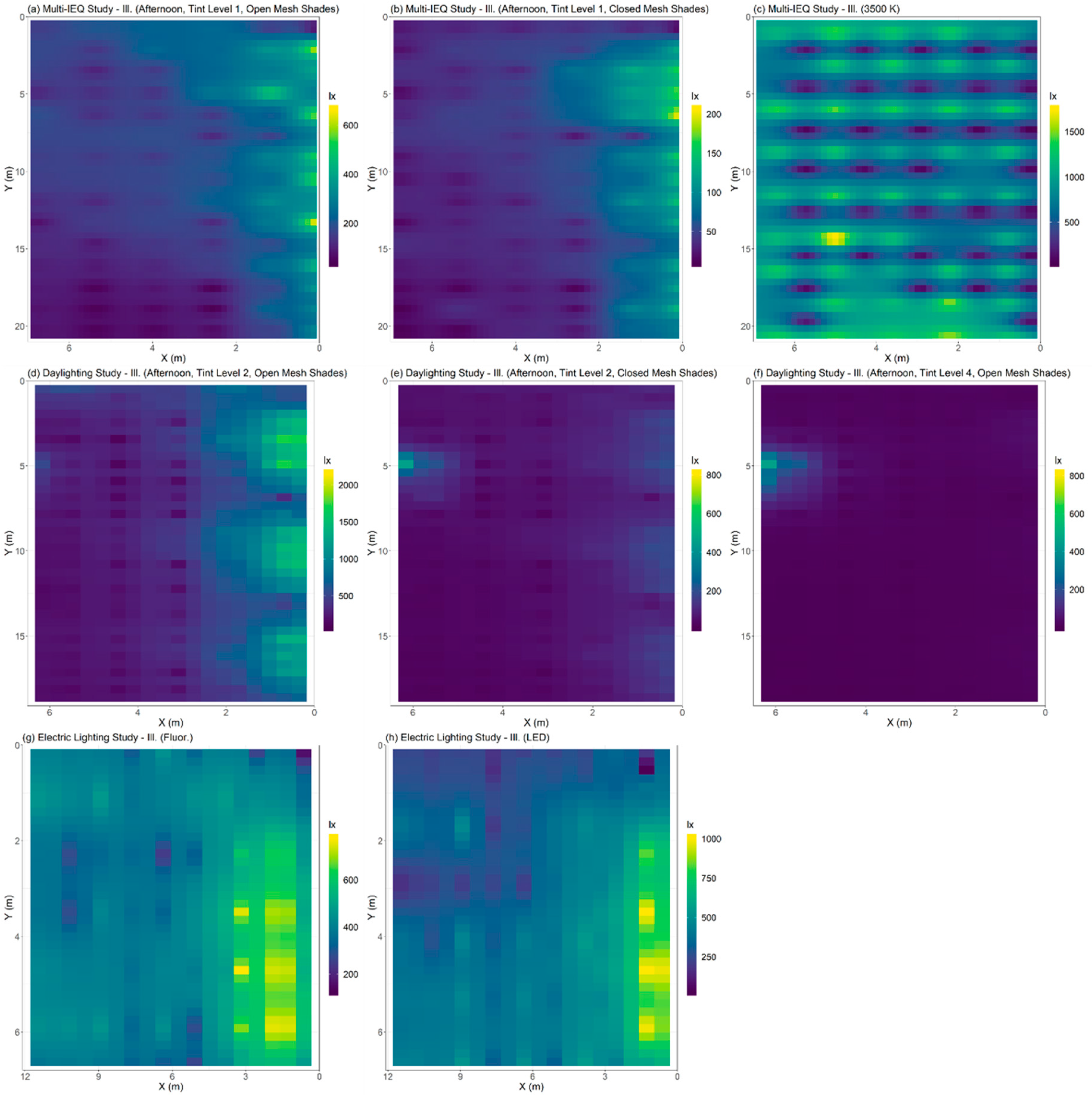
2.3.2. Spatial IEQ Assessments

While wireless sensor networks are well suited to describe temporal variability in experimental conditions at individual points, for factors like light and audio, it is useful to supplement point-measures with a spatial mapping of environmental conditions under experimentally representative settings. This is especially useful when conditions vary over distances shorter than the distance between sensors or if no wireless sensor was available for continuously measuring the environmental factor of interest. Three types of spatial assessments were conducted: Lighting, sound, and surface temperatures. Surface temperature data collection methods are included in the supplement.

Spatial lighting assessments were conducted for all three studies. The spatial variability of electrical lighting was assessed during the multi-IEQ and electric light studies for each lighting set point, while the spatial variability of natural light was assessed during the multi-IEQ and daylighting studies. In all spatial lighting assessments, an illuminance spectrophotometer (CL-500A) was used to measure illuminance, CCT, and spectral power density (SPD, 360–780 nm at 1 nm intervals) in the horizontal plane at a height of 0.88 m over a grid of sampling points (see Figure S1). Electric lighting sampling points were designed to measure light conditions between overhead luminaires (minimum), directly under luminaires (maximum), and at intermediary points between maximums and minimums. Natural light spatial assessments were conducted on sunny days during the morning (08:00–11:00) and afternoon (12:00–15:00) with the façade set to conditions representative of the range of conditions expected to occur during the studies. For more details of natural light spatial sampling, see the Supplemental Information. While not comprehensive spatially, desk-level measurements of horizontal electric lighting conditions were collected prior to the daylighting and electric lighting studies using the spectrophotometer to accurately set an average electrical lighting set point across desks, a requirement that was not included in the multi-IEQ study design.

A spatial assessment of sound levels was conducted during the multi-IEQ study to evaluate background noise levels and quantify spatial differences in sound-masking introduced into the office with in-ceiling speakers. Spatial sound level sampling was designed similarly to the spatial lighting assessment, with measurements collected between speakers (minimum), under speakers (maximum), and at intermediary points between maximums and minimums, as shown in Figure S2. An acoustic analyzer (XL2) with a 1-second sample rate collected 30 (white noise) or 60 (office sounds) seconds of sound level data at each sampling point and a height of 0.76 m for the five sound masking conditions: 1. No sound masking (background noise levels), 2. office sounds 1, 3. office sounds 2, 4. low-volume white noise, and 5. high-volume white noise. The ventilation system was set to operate at the same supply flow rate throughout sampling to limit variability in HVAC-related background noise. Inverse distance weighting was used for spatial lighting and sound assessments to interpolate values for data visualization.

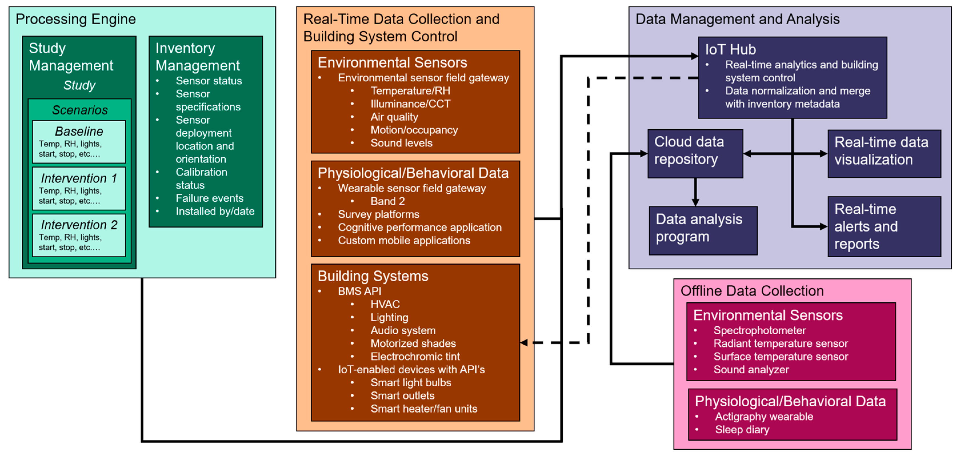
2.3.3. Cloud Infrastructure and Data Analysis

The underlying software and hardware infrastructure implemented at the lab for data management and control of building systems and other smart devices, referred to generally as “actuators”, consists of four primary components, shown in Figure 2: A cloud-based processing engine; the physical sensors, mobile device applications, and actuators that collect data and control building systems; offline sensors with data logged internally and downloaded at regular intervals; and the data management and analysis pipeline. The processing engine was designed as both a study management and inventory management tool for creating a database describing all components of a research investigation. Within this engine, a series of experimental conditions (“Scenarios” in Figure 2) can be programmed to occur in the modules within a specific time frame according to a study’s design, during which the building systems are maintained at prescribed set points by connecting the processing engine to actuators with an internet of things (IoT) hub (dashed line in Figure 2). Parallel to study management in the processing engine is the inventory management, where both historical and current study deployment metadata of sensors and actuators are stored. Deployment metadata include sensor location, orientation, installation method, calibration status, and failure events.

Data collection is split between human and non-human types, with additional security practices implemented for human-subject data to maintain participant anonymity and ensure data security (e.g., HIPAA-compliant cloud repository). Field gateways for environmental sensor networks, survey platforms, and custom mobile device applications are set up to communicate with the IoT hub for data ingestion after data are normalized and merged with inventory metadata. Similarly, the BMS and other actuators are connected to the cloud via custom connector applications that utilize application programming interfaces (APIs) to communicate with these devices. Sensor communication with the IoT hub is unidirectional (ingest), while actuator communication with the IoT hub is bidirectional (ingest, command). Data are visualized in real time using an online data visualization platform (PowerBI, Microsoft Corp., Redmond, WA, USA), which is useful for checking set points are met and identifying sensor issues. Alerts and data collection reports can also be generated in real time to assist with study operation. Data collected by offline sensors are uploaded directly to the cloud repository following download from the device.

Beyond simply maintaining set points, coupling the IoT hub with real-time data analytics and BMS set points allows for experimental conditions to be defined with algorithmic rules for actuator control with time-based events and/or any incoming data stream to the IoT hub. Real-time analytics also allow data to be transformed prior to ingestion into the data repository, for example to apply calibration equations, calculate moving averages, and convert between units.

Data were processed and analyzed in R [71]. Data processing included filtering data from sensor malfunctions, applying calibration equations, and deriving hourly summary statistics. Two desk-level air temperature/RH sensors, one window-level illuminance sensor, and one background-level illuminance sensor deployed during the multi-IEQ study had connection issues and were removed during processing due to poor data coverage. Statistical summaries and assessments of spatial and temporal variability were limited to weekdays during working hours, 06:00–18:00 CST.

3. Results and Discussion

3.1. Statistical Summary

The geometric mean (± arithmetic standard deviation, SD) of data from environmental sensors, HVAC air flow rates, and AHU return air RH for each experimental condition during work hours (06:00–18:00) are summarized in

Table 3. Geometric mean (±SD) of environmental conditions and observation numbers (N) measured by sensor networks and building systems during work hours (06:00–18:00) during the multi-IEQ study.

Multi-IEQ Study
Environmental Measurement	Near-Optimal (Baseline)	Optimal	Sub-Optimal 1	Mixed 1	Sub-Optimal 2	Mixed 2
(Sensor No., Units)	Geometric Mean ± SD (N)
AHU Air Flow (N = 1, CFM)	992 ± 182 (54,006)	962 ± 177 (52,175)	1054 ± 42 (48,878)	752 ± 288 (44,814)	1031 ± 76 (3840)	774 ± 250 (4258)
VAV Air Flow (N = 3, CFM)	353 ± 88 (65,601)	336 ± 97 (65,930)	388 ± 49 (59,556)	249 ± 133 (48,419)	396 ± 65 (10,106)	212 ± 120 (8967)
AHU Return RH (N = 1, %RH)	44 ± 3 (1797)	45 ± 6 (2706)	48 ± 3 (1087)	44 ± 4 (1114)	48 ± 4 (1041)	44 ± 3 (900)
Thermostat Temp. (N = 3, °C)	22.5 ± 0.8 (5112)	22.0 ± 0.9 (7604)	20.6 ± 0.7 (2855)	23.7 ± 0.7 (2879)	20.9 ± 1.5 (3139)	23.4 ± 0.7 (2342)
Desk Temp. (N = 7, °C)	24.1 ± 1.7 (17,474)	23.5 ± 1.6 (26,970)	22.0 ± 1.7 (9305)	25.4 ± 1.6 (9647)	22.0 ± 1.4 (9758)	25.1 ± 1.5 (8915)
Window Temp. (N = 3, °C)	23.5 ± 2.4 (4605)	22.4 ± 2.1 (6377)	24.3 ± 3.8 (2757)	24.7 ± 2.3 (2299)	22.2 ± 2.8 (2784)	24.1 ± 1.6 (2315)
Wearable Air Temp. (N = 8, °C)	30.3 ± 1.6 (23,024)	29.7 ± 1.7 (35,682)	29.2 ± 1.7 (12,852)	31.0 ± 1.6 (16,470)	28.9 ± 1.9 (14,866)	30.9 ± 1.5 (16,929)
Wearable Skin Temp. (N = 8, °C)	31.6 ± 1.3 (22,396)	31.1 ± 1.3 (35,472)	30.5 ± 1.3 (12,719)	32.3 ± 1.2 (16,406)	30.6 ± 1.2 (14,794)	32.2 ± 1.1 (16,876)
Desk RH (N = 7, %RH)	41.2 ± 4.3 (17,473)	43.9 ± 6.1 (26,966)	48.3 ± 4.3 (9305)	38.2 ± 3.5 (9648)	48.3 ± 5.0 (9758)	40.3 ± 3.8 (8915)
Desk Illum. (N = 9, lx)	385 ± 601 (10,615)	275 ± 466 (14,593)	154 ± 358 (5938)	367 ± 593 (6504)	277 ± 510 (5469)	340 ± 513 (4649)
Window Illum. (N = 7, lx)	2555 ± 9851 (9193)	557 ± 1662 (12,658)	57 ± 2625 (4800)	2112 ± 8954 (5011)	23 ± 143 (4765)	564 ± 1580 (3608)
Wearable Illuminance (N = 8, lx)	80 ± 552 (23,483)	54 ± 200 (35,767)	56 ± 145 (12,903)	77 ± 573 (16,510)	57 ± 140 (14,904)	70 ± 211 (16,982)
Near-Desk CO2 (N = 4, ppm)	512 ± 61 (53,222)	512 ± 59 (80,288)	515 ± 58 (28,645)	530 ± 70 (29,872)	508 ± 49 (29,866)	533 ± 66 (25,918)
Background CO2 (N = 2, ppm)	486 ± 70 (17,018)	484 ± 58 (27,073)	514 ± 60 (11,192)	516 ± 60 (11,169)	480 ± 47 (11,174)	503 ± 68 (9239)
External CO2 (N = 1, ppm)	467 ± 67 (13,487)	481 ± 55 (20,467)	466 ± 52 (7475)	456 ± 56 (7474)	473 ± 34 (7469)	472 ± 39 (6486)
Desk Sound Level * (N = 1, dBA)	46.9 ± 4.3 (224)	46.4 ± 4.6 (377)	46.9 ± 4.5 (130)	46.4 ± 4.4 (130)	47.2 ± 3.2 (130)	46.1 ± 3.9 (130)

* Sound level data were summarized to hourly arithmetic averages of “LAeq_dt” prior to calculation of statistical summaries per scene, whereas statistical summaries of all other data sets were derived from raw data time series.

and

Table 4. Geometric mean (± SD) of environmental conditions and observation numbers (N) measured by sensor networks and building systems during work hours (06:00–18:00) during the daylighting and electric lighting studies.

Daylighting Study				Electric Lighting Study
Environmental Measurement	No View (Baseline)	Mesh Shades	Dynamic Tint	Environmental Measurement	Fluorescent (Baseline)	LED
(Sensor No., Units)	Geometric Mean ± SD (N)			(Sensor No., Units)	Geometric Mean ± SD (N)
AHU Air Flow (N = 1, CFM)	479 ± 193 (10,017)	606 ± 296 (13,795)	628 ± 330 (14,603)	-	-	-
VAV Air Flow (N = 3, CFM)	190 ± 129 (16,266)	213 ± 145 (17,042)	188 ± 147 (20,590)	VAV Air Flow (N = 2, CFM)	133 ± 70 (23,171)	106 ± 39 (24,942)
AHU Return RH (N = 1, %RH)	44 ± 2 (3118)	43 ± 3 (3713)	43 ± 1 (3338)	AHU Return RH (N = 1, %RH)	47 ± 1 (5597)	46 ± 2 (7064)
Thermostat Temp. (N = 3, °C)	23.3 ± 0.5 (7842)	23.6 ± 0.5 (9674)	23.6 ± 0.5 (9565)	Thermostat Temp. (N = 2, °C)	22.3 ± 0.3 (5923)	22.0 ± 0.4 (7293)
Desktop Temp. (N = 10, °C)	23.8 ± 0.9 (15,741)	24.5 ± 1.3 (15,512)	24.7 ± 1.1 (15,710)	Desktop Temp. (N = 4, °C)	22.4 ± 0.4 (46,476)	22.0 ± 0.5 (57,611)
Window Temp. (N = 8, °C)	25.5 ± 4.9 (12,495)	25.8 ± 4.2 (12,326)	26.6 ± 3.8 (12,496)	-	-	-
Wall Temp. (N = 8, °C)	23.2 ± 0.8 (12,785)	23.8 ± 1.2 (12,658)	23.9 ± 1.0 (12,753)	Wall Temp. (N = 7, °C)	22.3 ± 0.9 (21,856)	21.4 ± 1.3 (27,026)
Desktop RH (N = 10, %RH)	39.6 ± 2.9 (15,741)	37.6 ± 3.0 (15,512)	37.7 ± 2.3 (15,710)	Desktop RH (N = 4, %RH)	41.9 ± 0.9 (46,476)	42.4 ± 1.8 (57,612)
Desktop Illum. (N = 10, lx)	291 ± 45 (128,577)	457 ± 539 (128,475)	463 ± 450 (130,095)	Desktop Illum. (N = 10, lx)	230 ± 92 (140,324)	295 ± 105 (167,451)
Desktop Illum. (CCT sensors, N = 10, lx)	290 ± 40 (130,208)	689 ± 2865 (130,496)	724 ± 1468 (130,930)	Desktop Illum. (CCT sensors, N = 10, lx)	281 ± 83 (121,920)	298 ± 105 (150,652)
Window Illum. (N = 16, lx)	26 ± 115 (25,340)	1226 ± 6035 (24,404)	1020 ± 3550 (24,780)	-	-	-
Window Illum. (CCT sensors, N = 8, lx)	19 ± 365 (12,208)	1673 ± 6654 (11,994)	1296 ± 2776 (12,247)	-	-	-
Desktop CCT (N = 10, K)	4290 ± 121 (130,208)	4786 ± 474 (130,497)	5216 ± 728 * (130,931)	Desktop CCT (N = 10, K)	3515 ± 353 (121,923)	5967 ± 173 (150,653)
Window CCT (N = 8, K)	9300 ± 4660 * (11,832)	5537 ± 810 (11,994)	6365 ± 2572 * (12,219)	-	-	-

* Window CCT sensors and, less frequently, desk CCT sensors responded erratically at darker tint levels, 3 and 4, impacting all data in the no view condition (level 4) and data collected during morning periods of the dynamic tint condition. Desk-level sensors were less impacted than window-level sensors.

. Tables S2 and S3 contain additional statistical summaries for the multi-IEQ and daylighting/electric lighting studies, respectively, including arithmetic mean, geometric standard deviation (GSD), maximum, and minimum values, and Figures S3–S7 describe the distributions of environmental data for all conditions of the three experiments, including HVAC operational parameters (Figure S3), thermal conditions (Figure S4), lighting conditions (Figure S5), sound levels and CO₂ concentrations (Figure S6), and environmental data from wearable sensors (Figure S7). As these figures demonstrate, distributions tended to be skewed, leading to the reporting of geometric means, though arithmetic standard deviation is included in Table 3 instead of GSD to simplify interpretation of parameter variability.

Experimental conditions with decreased temperature set points (sub-optimal 1, sub-optimal 2) and increased heat load from open windows (near-optimal, optimal, mesh shades, and dynamic tint) tended to increase AHU and VAV flow rates relative to other conditions, though spot checks of air velocity (Q-Trak 964 Probe, TSI, Inc.) below supply diffusers at elevated VAV flow rates (400 CFM) did not exceed 0.14 m/s and averaged 0.03±0.01 m/s, suggesting minimal impact on thermal comfort. As demonstrated in further detail below, increased variability in desk-level temperature, RH, illuminance, and CCT levels were detected in all conditions in which windows were open. Low temperature set points (19.4 °C) were not met on average during the multi-IEQ study, with thermostat temperatures 1.2–1.5 °C higher and desk-level sensors 2.6 °C higher than set points. Other temperature set points (21.7, 22.8, and 23.9 °C) were met within 1 °C at both the desk and thermostat levels. Relative humidity measured at the AHU level was generally higher than the set point by 3–8 %RH, though desk-level measurements tended to deviate less from the set point compared to return air RH. Desk-level illuminance set points were met within 9, 20, and 45 lx during the no view, fluorescent, and LED conditions when no natural light was present. While illuminance sensors and CCT/illuminance sensors generally agreed within the sensor calibration range, the two sensor types deviated at illuminance levels above the calibration range, resulting in the CCT/illuminance sensors reporting larger illuminance values than the illuminance-only sensors. The temporal and spatial analysis below reports data from illuminance sensors to summarize across conditions, as they were included in all studies.

Window-level and desk-level illuminance sensors reported the highest values with windows set to tint level 1 (near-optimal, mixed 1), followed by tint level 2 (mesh shades) and automated tinting conditions (optimal, mixed 2, and dynamic tint). Allowing participants to override tinting (dynamic tint) resulted in elevated window and desk-level illuminance compared to automated tint conditions without occupant control (optimal, mixed 2), which resulted in more similar average daylight levels between conditions with natural light during the daylighting study than during the multi-IEQ study. Desk-level CCT generally showed good agreement with set points within 300 K. Elevated CCT in the LED condition relative to set point is likely a sensor inaccuracy issue, as desk-level spectrophotometer readings averaged 5007 ± 102 K during lighting setup. Elevated CCT was measured when windows were open, increasing by 786 and 1216 K during the mesh shades and dynamic tint conditions, respectively, relative to the no view condition.

The temperature variability (SD) detected during the windowless experimental conditions (sub-optimal 1, sub-optimal 2, no view, fluorescent, and LED) of 0.5–1.5 °C is generally above the variability reported in well-controlled chamber and lab studies, which tend to be less than 0.5 °C and can be as low as 0.1 °C due to shorter exposure periods with smaller room air volume and more precise thermal system controls [72,73,74,75]. Compared to field studies and lab-based simulated offices, the temperature variability measured here is similar [57,58,74,76,77,78], and as is shown below, tended to exhibit diurnal variability driven by solar radiation and façade design, as is expected in most buildings in moderate and colder climates. The average relative humidity levels maintained in all experiments stayed in the range of 37–49 %RH, within the recommended limits of 30–60 %RH, and the amount of variability in RH was comparable to other chamber and field studies [58,72,73,74,75,78].

We note that in previous investigations with multiple sensors deployed, the variability contributed to by temporal variability is rarely considered separately from spatial variability. In the summary statistics above, much of the elevated variability in the described living lab studies can be attributed to spatial variability, rather than ability to maintain set points over time, whereas in chamber studies, there are rarely considerations of spatial variability due to smaller size and in field studies, rarely are enough data collected to accurately assess such trends. In the sections below, spatial and temporal variability factors are split by comparing diurnal trends of individual sensors and by comparing diurnal trends of all sensors across experimental conditions. Details of changes in sensor sample rates between experiments and sensor communication issues can be found in the Supplemental Information.

Other considerations for large-scale environmental sensor deployments include completeness statistics for summarizing data on different time scales. For example, the U.S. E.P.A. has a threshold of 75–90% completeness for annual, daily, and hourly summary statistics to be valid [79], a threshold that should be adopted by IEQ researchers to ensure data are representative of the time interval over which they are summarizing. While a large community of scientists are tackling issues of low-cost air quality sensor calibration and operation, much less focus has been placed on improving low-cost sensor accuracy and availability for other IEQ factors. A recent publication series describes the design and performance of the SAMBA environmental monitoring platform, including reference instrument comparisons of air temperature, humidity, globe temperature, air velocity, CO₂, carbon monoxide, particulate matter, formaldehyde, sound level, and illuminance [80,81]. Such comparisons are essential for validating IEQ measurement techniques. Inaccurate environmental sensors greatly limit the ability to detect spatial variability, as biases between sensors cannot be easily distinguished from spatial differences.

A limiting factor in these studies is that environmental monitoring only occurred in the lab modules, and environmental data were only relevant to participant experiences/exposures while they were present in the office. Future experiments will aim to include environmental monitoring of control group workspaces, as well as extend lab group monitoring to the home and other environments using field-deployable environmental sensor suites. Wearable environmental sensors are able to report more accurately the environmental conditions to which occupants are physically exposed and may be preferable to desk-level proxies [60].

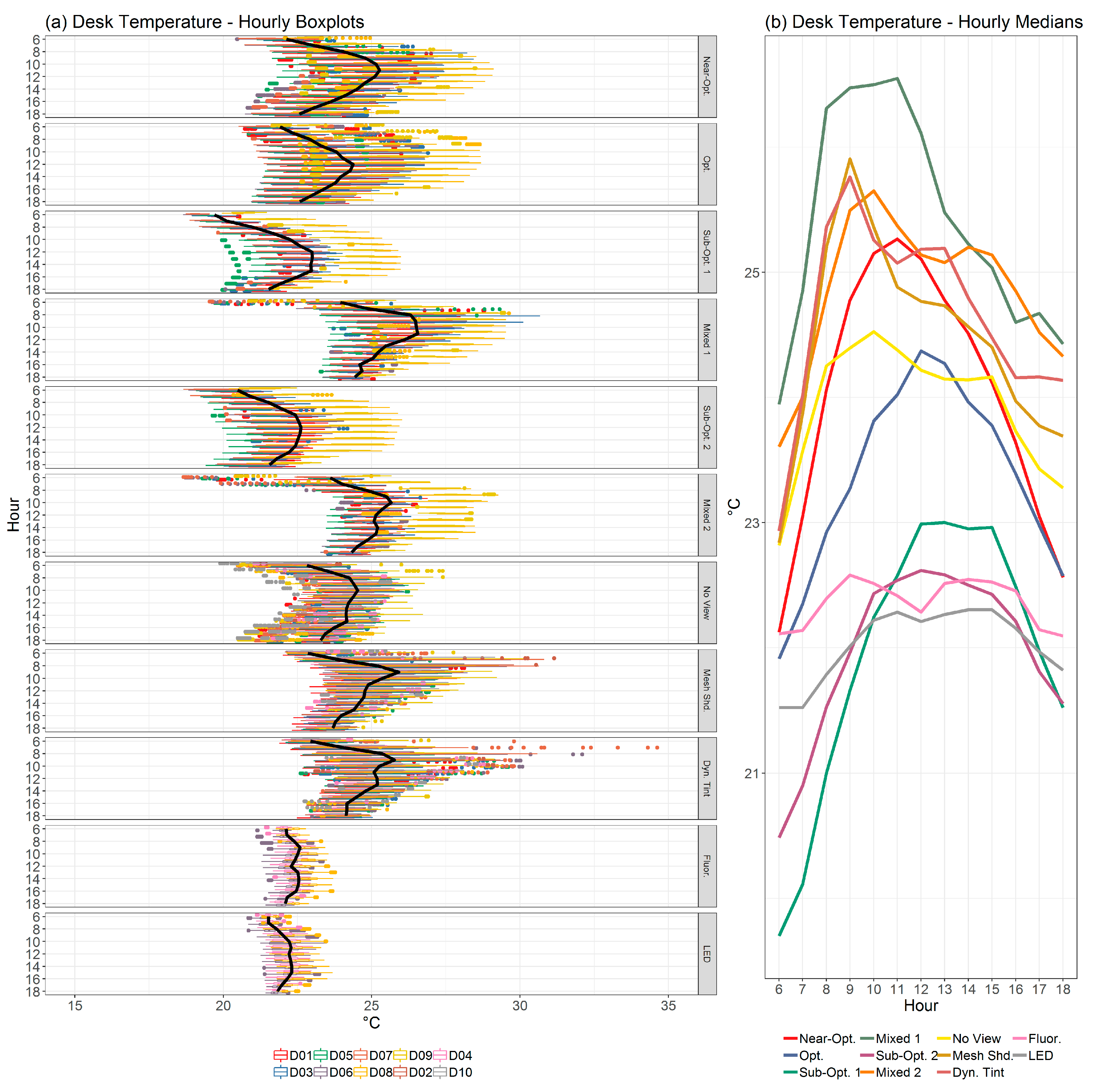
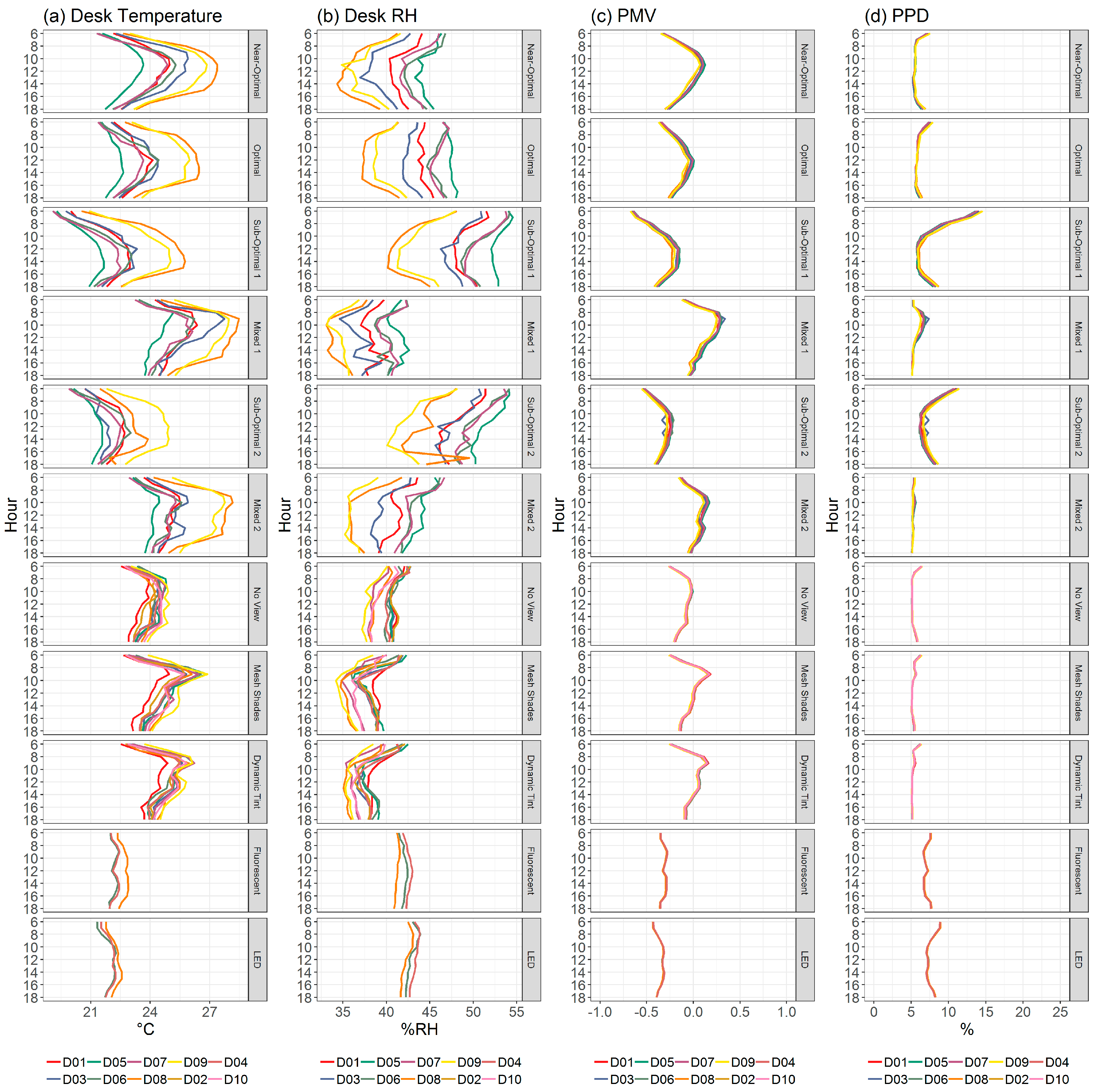
3.2. Thermal Conditions

Significant desk-level deviations from temperature setpoints of up to 3 °C occurred in all experimental conditions where window shades were open, as shown in Figure 3, and about 1 °C of diurnal differences were detected in conditions without windows and a north facing façade (LED and fluorescent experimental conditions). Set points were generally met at the start of the day, even for low temperature set points of 19.4 °C, but they rapidly increased as the modules became occupied and as solar radiation began heating the building. Experimental conditions with automated window tinting (optimal, mixed 2, and dynamic tint) demonstrated a time-shifted peak in temperature, shifting from 09:00 to about 12:00. This trend is also observed at the window level (Figure S8).

Figure 4 depicts the spatial variability in desk air temperature, RH, predicted mean vote (PMV), and predicted percentage dissatisfied (PPD), as calculated using desk-level temperature and humidity assuming a metabolic rate of 1.2 met, mean radiant temperature of 22 °C, clothing level of 1, and air velocity of 0.2 m/s [82,83], by experimental condition in each study. There was a notable reduction in spatial variability in thermal conditions between the multi-IEQ study and latter studies, resulting in less between-participant variability in thermal comfort predictions. As shown, the set point temperature was not the temperature participants physically experienced while at their desks for most of the day, highlighting the importance of near-body environmental measurements to accurately detect exposure conditions. Temperature set point changes tended to shift the entire diurnal profile such that the intended between-scene temperature differences were maintained. PMV values tended to stay between ±0.5, and PPD values were usually below 10%, suggesting that thermally comfortable environments were provided to participants. Temporal variability in PMV–PPD indices was significantly larger than spatial differences.

Of note is the impact of desk layout on temperatures at desks D08 and D09 in the multi-IEQ study, which were nearly fully enclosed in cubicle walls and shared a single supply diffuser with two other desks, resulting in these desks experiencing temperatures about 2 °C higher than others. There was a comparably lower temperature detected at an unoccupied desk, D05, compared to all other sensors in the multi-IEQ study, suggesting desk-level heat sources (computers, monitors) and the human body’s thermal plume are likely to be impacting the desk-level spatial variability observed in these studies. Desk D01 in the daylighting study had much of the east façade blocked by adjacent desks and walls, resulting in slightly lower desk-level temperatures compared to all other desks due to reduced radiant heat reaching this desk. Humidification systems tended to not be able to maintain relative humidity set points during morning periods when temperatures were rapidly increasing, with RH dropping by up to 5 %RH from 06:00–10:00. Future studies will aim to utilize a set point of 45–50%RH to help ensure that these morning reductions do not cause desk-level RH to stray from the recommended 30–60 %RH range.

In lieu of continuous radiant temperature measurements, surface temperatures were measured throughout the office space during the daylighting study. As with air temperature data, surface temperatures along the east façade were elevated during morning by solar heating, though inconsistent patterns were observed for the impact of meteorology, as shown in Figure S9. For internal surfaces and along the north wall, surface temperatures maintained a consistent temperature throughout the day.

A correlation analysis was conducted between desk-level air temperature and wearable air and skin temperatures to evaluate whether desk-level temperature was predictive of personal experience of temperature as sensed by a wrist-worn device. Figure S10 depicts the correlation between desk and wearable temperature readings, showing that while desk temperatures were consistently correlated with themselves, about half of the wearable devices were moderately correlated with desk temperatures, while the other half of the wearable devices demonstrated low to no correlation with desk temperatures but in some cases, moderate correlation with other wearables. Confounding effects that may explain some of the deviation from desk-level measurements include spending time away from the desk, sleeves covering the device and increasing thermal insulation, differences in physiology (e.g., met rate), and human behaviors like wearing a blanket.

The human elements of thermal comfort, metabolic rate and amount of clothing worn were not characterized in these studies, as accurate thermal comfort modeling was not an experimental aim. Metabolic rate can be estimated based on expected work task type, but investigators should also consider a wearable device capable of directly measuring metabolic rate [84] or environmental proxies of metabolic rate, such as temporal variability of CO₂ generation coupled with air exchange rate measurements [85], to assess this important physiological parameter in real time. Such data could one day be incorporated in thermal control systems, allowing buildings to further adapt to occupant needs. There are no continuous measurement devices capable of monitoring clothing level, which in prior studies is assumed based on visual inspection or addressed with survey tools.

As the adaptive thermal comfort model makes clear, seasonal variability in thermal comfort is somewhat driven by ambient temperature and occupants altering clothing type [86]. One limitation of these studies is that they all took place during a similar time of year (May–September), representing summer and fall conditions but not colder winter conditions.

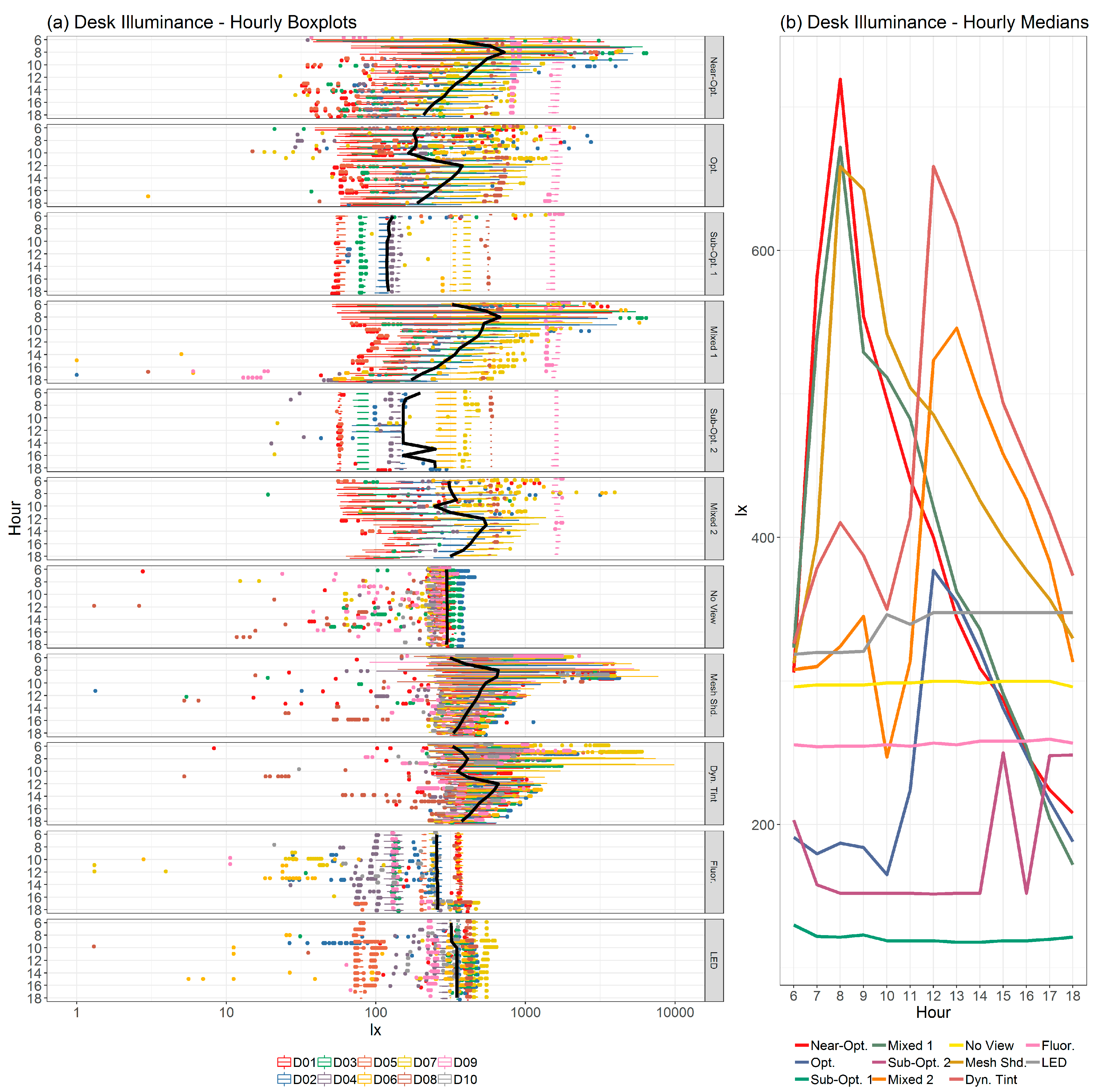
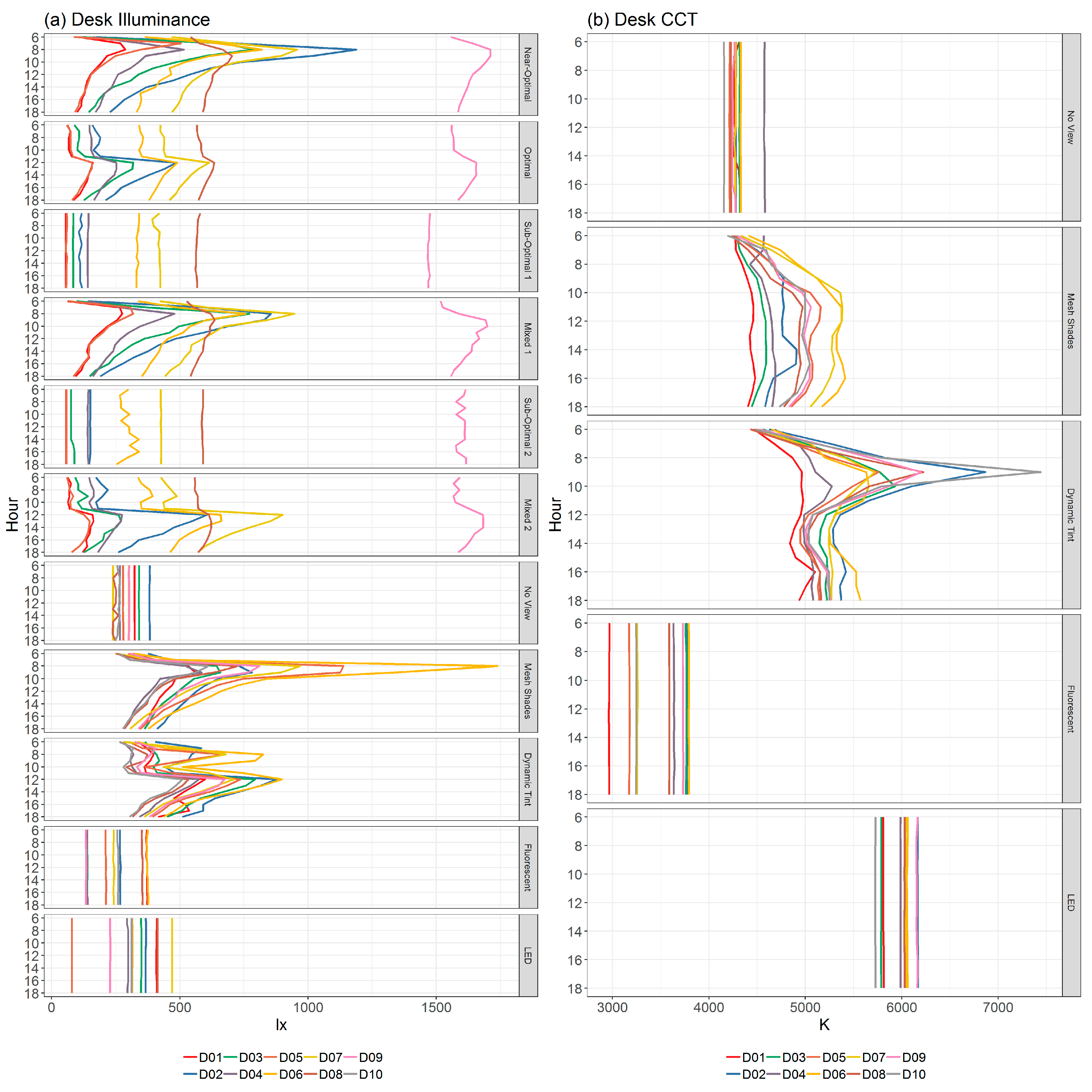
3.3. Lighting Conditions

As shown in Figure 5, temporal variability in desk-level illuminance was driven by façade control type, as all experimental conditions in which mesh shades were allowed to be adjusted by participants (near-optimal, mixed 1, and mesh shades) without automated tinting resulted in peak illuminance during the morning, while automated tint conditions (optimal, mixed 2, and dynamic tint) shifted peak illuminance to later in the day (11:00–14:00). Temporal variability in desk-level CCT, included in Figure S11, demonstrated the opposite pattern to illuminance, with darker tint levels increasing CCT during the morning peak in window-level illuminance, and desk-level CCT during the mesh shades condition following the diurnal pattern of solar radiation. Figure S12 shows temporal patterns in window illuminance, again highlighting the significant reductions in morning illuminance when automated tint was used. In windowless conditions during which tint levels were set to 4, window-level sensors indicated a two orders-of-magnitude reduction in penetration of light through window surfaces. Conditions without natural lighting (sub-optimal 1, sub-optimal 2, no view, fluorescent, and LED) demonstrated temporal stability in illuminance and CCT (Figure S11). Some desk-level variability in illuminance during electric light-only conditions can be attributed to changes in desk height of sit-stand desk workstations, especially notable during the multi-IEQ study. Recent studies at the lab have dealt with this uncertainty by either locking desks at a single height following ergonomic fitting or by installing desk-height sensors and developing desk height-electric lighting illuminance relationships.

The can-lighting system used in the multi-IEQ study resulted in highly spatially variable illuminance levels, as demonstrated by the range of desk-level illuminance in Figure 6 during the sub-optimal 1 and sub-optimal 2 conditions and in the spatial assessment below. Of note is D09, as this sensor was on a desk that was always in the standing position (1.1 m desk height versus 0.75 m) and was placed directly under a lamp during sensor deployment, resulting in dramatically increased average light levels indicated by this sensor. Replacing the can-lighting system with linear troffers for the daylighting study reduced desk-to-desk variability in electric light levels, demonstrated in the no view condition in Figure 6a. This highlights the importance of understanding spatial variability in lighting conditions during lighting design and sensor placement, as under highly variable conditions, there may not be an optimal sensor placement and supplemental spatial measurements under representative conditions may be necessary to characterize the lighting environment. Temporal variability, which can be leveraged in façade and electric lighting controls, may still be adequately characterized in such a situation.

Taller partition height and smaller troffer sizes drove illuminance sensors in the electric lighting study to detect more spatial variability than during the no view conditions of the daylighting study. For the electric lighting study, two different sets of luminaires were installed parallel to each other (Figure S1c), which resulted in different spatial variability patterns between the fluorescent and LED conditions. While there were experimental design reasons for this decision (e.g., inability to exchange fluorescent and LED troffers between experiments), it is important to address the impact of such decisions for future experimental designs that rely on consistent exposures to environmental conditions in determining their impact on human outcomes.

Spatial variability maps of natural and electric lighting during the three studies are included in Figure 7 and Figure S13. Comparing the spatial variability indicated in Figure 7c,g–h demonstrates the dramatic reduction in variability when troffer-style luminaires were installed instead of can-type. Results from natural light variability assessments during the multi-IEQ study (Figure 7a) were used to estimate optimal desk placement during the subsequent daylighting study. While closing mesh shades greatly reduced natural light, general spatial variability patterns were maintained (Figure 7b,e), while tinting to level 4 essentially removed completely the impact of natural light in the office space (Figure 7f). Note that the electric lights in the conference room during the electric lighting study were adjustable by participants as needed and were set to their maximum value during spatial lighting sampling, whereas the rest of the office lights were set such that desks received on average 250 lx.

Spatial variability of CCT over all measured conditions is included in Figure S14, showing some light-to-light variability in CCT during the multi-IEQ study as well as the significant impact of tint level 4 on measured CCT from natural light penetration. In cases with low levels of tint and some natural light penetration, CCT gradients generally followed the same pattern as illuminance. Note that light measurements in the low light conditions (mesh shades closed and tint level 4) were collected with an undercabinet light in the kitchen turn on, as otherwise visibility was too low, which impacted spatial assessments of illuminance and CCT on the west side of the office.

A detailed description of how façades were controlled by occupants and how this control resulted in variability in desk-level illuminance and temperature is included in the supplement (see Façade Control section and Figures S16–S18). In short, dynamic tinting lowered desk-level air temperatures while also reducing illuminance levels, whereas mesh shading reduced illuminance but did not impact desk-level temperatures. As with thermal measurements, the impact of seasonal differences in solar radiation are not possible to be assessed, as these measurements focused on the summer and fall. Glare may also vary with seasonal patterns in the sun’s path.

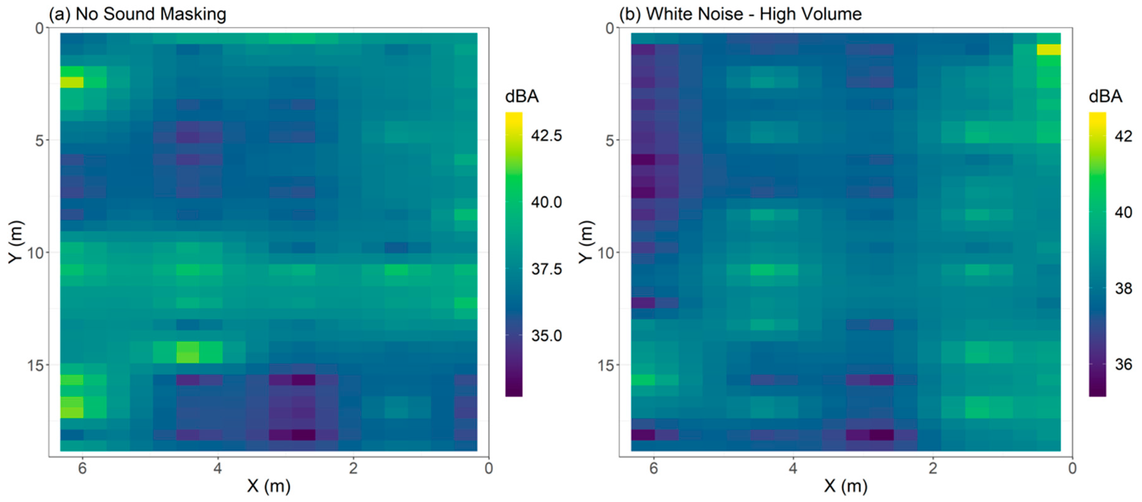
3.4. Auditory Conditions

Spatial assessments were conducted to evaluate the sound masking that was used during the multi-IEQ study. As Figure 8a shows, background sound levels varied from about 32 to 43 dBA, which are typical or slightly quieter than is often reported in modern offices [87]. It is hypothesized that the line of elevated background noise at the center of the modules running west to east is the result of duct noise penetrating through the ceiling tiles, as supply air ducts for two of the three modules run through this region. Air supply diffusers were also identified as sources of background noise, though measurements under diffusers near windows were also likely impacted by external noise penetration. The spatial assessment for the high-volume white noise condition is included in Figure 8b and clearly shows the speaker positions and loudness gradients in a similar range to noise levels observed in the background condition. Following the multi-IEQ study, speakers were replaced with alternatives that provided a wider coverage angle than those used in this study to minimize spatial variability in sound masking. There were no detectable average increases in sound levels when sound masking was turned on as assessed by dBA-based summaries of spatial variability, though by plotting specific frequency bands, especially in the mid-to-high frequency ranges (>500 Hz), the introduced sound masking audio is apparent. Figure S19 includes the spatial variability in sound levels for the low volume white noise condition, which also depicts speaker location, and the office sounds conditions, which mirror the background noise measurements.

The temporal variability in sound levels during the multi-IEQ study is shown in Figure S20. Sound levels followed general occupancy patterns, also seen below in CO₂ concentrations, with daytime values usually ranging from 45 to 50 dBA, which is typical of a modern office. While duct air flow patterns were observed to impact spatial sound levels above, the time series of office noise levels from desk D05 does not follow the pattern observed in VAV air flow, included in Figure S21, which tended to increase well after the office became occupied in the morning and stay elevated throughout the workday, whereas sound levels increased immediately upon occupancy and decreased gradually in the afternoon. Occupant-produced sounds also tended to be in the higher frequencies, as shown in the audio spectrum time series in Figure S22. Therefore, it is estimated that most of the sound level increase measured during work hours was a direct result of occupant-generated noise, validated by weekday–weekend comparisons of sound levels (e.g., Figure S22). Daily sound level patterns did not change as background audio was introduced into the space, though as with the spatial sampling, the impact from background audio is evident at higher frequencies.

As highlighted in Jamrozik et al., 2018, participants’ experiences of the office were highly impacted by the introduction of background audio, despite environmental sensors not detecting a difference in sound-level conditions. This is a major limitation of sound-level based inference for sound sources which carry speech context, which is particularly disruptive, or for sounds that are annoying (e.g., telephones ringing) or jarring (e.g., impact sounds from dropping an object on the floor), as compared to historical measurements of background or industrial noise loudness. There are metrics meant to evaluate the impact of speech in a room, such as the speech intelligibility index, but such measurements are better at characterizing the acoustic properties of a space rather than quantifying the impact of actual human-generated sounds in time. Machine learning algorithms are a promising solution to this dilemma, as audio can be analyzed in real time for context and emotional content, as well as decipher speech-generated sounds from other background sounds [88,89].

3.5. Carbon Dioxide Concentrations

CO₂ concentrations provide an indication of the effectiveness of the ventilation system at removing human bioeffluents and other pollutants. Figure S23 depicts daily variability in CO₂ concentrations measured during the multi-IEQ study, showing general occupancy patterns matching those identified with the sound level meter. CO₂ concentrations were maintained well within acceptable limits and rarely exceeded 800 ppm. Diurnal patterns in CO₂ corresponded with temperature set points, with elevated temperature set points that resulted in lower AHU and VAV flow rates having higher peak morning CO₂ concentrations than during other temperature set point conditions. While CO₂ concentrations were maintained well within occupational exposure limits, participants reported less satisfaction with air quality and circulation during the sub-optimal 1, sub-optimal 2, and mixed 2 conditions. This result is hypothesized to be impacted by the overall poor perception of these conditions, created by removing natural light and introducing background sounds, rather than being attributed to actual degradation in air quality.

4. Conclusions

Through analysis of environmental sensor data collected during three office-based human subject experiments, we demonstrated the ability of a living lab to simulate a real office space to conduct human-centric building science research over a wide range of experimental conditions and IEQ set points. While chamber-based studies may be capable of reduced variability in environmental conditions, here we demonstrated that a living lab can simulate a wide range of building designs with more realistic interior designs over longer periods with more natural temporal variability in environmental conditions. One difficult aspect of the living lab approach is providing all participants with a similar IEQ experience, which requires reducing spatial variability in environmental exposures as much as possible. By adjusting building system design (e.g., luminaire type) and interior layout after the multi-IEQ study, spatial variability in thermal and lighting conditions were shown to be reduced in the daylighting and electric lighting studies.

While a high level of ecological validity is to be aimed for with living lab studies, successful experimental design often requires compromising realism with practical aspects of conducting research, such as balancing the need for accurate desk-level or personal exposure environmental data without detracting from the realism of the experimental. Such compromises also extend to human outcomes, such as assessing the frequency and length of surveys to prevent burn-out and selecting medical-grade wearables that are comfortable and easy to use to increase compliance.

As the living lab paradigm becomes more widespread, it is expected that additional facilities will be available for direct comparisons with other living lab-type approaches, though at this time there are few. SenseLab is an example that includes smaller chambers and an “experience room” that can be extensively remodeled in a similar manner to the Well Living Lab modules [51]. The Total Indoor Environmental Quality lab at the University of Syracuse approaches the realism of the office environment and is capable of precise thermal and air quality control for human-subject research [57].

While the living lab approach has many advantages, limitations of the Well Living Lab facility include: Lower cohort size relative to other methodologies (limited to 5 participants per module), requiring multiple cohorts to reach adequate sample size for some statistical comparisons; physical aspects of the building that may detract from the realism, such as entering a lab facility in a business building for a residential study, or detract from possible research scope (e.g., no southern or western façades); and continued need to improve upon and utilize standardized IEQ measurement methodologies. If the lab demonstrates building-based interventions to be effective, we plan to pursue large-scale follow-up field studies, in which capabilities developed within the lab environment will be extended outside the facility using mobile environmental sensing, surveying, and wearable data collection. An additional capability, building system monitoring and control, would also be pursued in such endeavors, porting as much of the living lab-approach into the field setting as possible. These research approaches could one day be scaled up to whole-building or city-wide living lab-type investigations.

Based on findings from this analysis, future living lab studies should carefully consider how to: (a) Simulate natural temporal variability in IEQ factors found in “typical offices” and other building typologies, (b) reduce spatial variability between desk-level environmental conditions such that inter-cohort variability in exposure is reduced, and (c) balance requirements of natural temporal variability and reduced spatial variability with other experimental design requirements, such as ability of participants to have control over building systems.

References

1. Klepeis, N.E.; Nelson, W.C.; Ott, W.R.; Robinson, J.P.; Tsang, A.M.; Switzer, P.; Behar, J.V.; Hern, S.C.; Engelmann, W.H. The National Human Activity Pattern Survey (NHAPS): A resource for assessing exposure to environmental pollutants. J. Expo. Sci. Environ. Epidemiol. 2001, 11, 231–252. [Google Scholar] [CrossRef] [PubMed]
2. Cedeño-Laurent, J.G.; Williams, A.; MacNaughton, P.; Cao, X.; Eitland, E.; Spengler, J.; Allen, J. Building Evidence for Health: Green Buildings, Current Science, and Future Challenges. Annu. Rev. Public Health 2018, 39, 291–308. [Google Scholar] [CrossRef] [PubMed]
3. Breysse, P.N.; Gant, J.L. The Importance of Housing for Healthy Populations and Communities. J. Public Health Manag. Pract. 2017, 23, 204–206. [Google Scholar] [CrossRef] [PubMed] [Green Version]
4. Allen, J.G.; MacNaughton, P.; Laurent, J.G.C.; Flanigan, S.S.; Eitland, E.S.; Spengler, J.D. Green Buildings and Health. Curr. Environ. Health Rep. 2015, 2, 250–258. [Google Scholar] [CrossRef] [PubMed] [Green Version]
5. Wang, Z.; de Dear, R.; Luo, M.; Lin, B.; He, Y.; Ghahramani, A.; Zhu, Y. Individual difference in thermal comfort: A literature review. Build. Environ. 2018, 138, 181–193. [Google Scholar] [CrossRef]
6. Reinten, J.; Braat-Eggen, P.E.; Hornikx, M.; Kort, H.S.M.; Kohlrausch, A. The indoor sound environment and human task performance: A literature review on the role of room acoustics. Build. Environ. 2017, 123, 315–332. [Google Scholar] [CrossRef]
7. Banbury, S.; Berry, D. Office noise and employee concentration: Identifying causes of disruption and potential improvements. Ergonomics 2005, 48, 25–37. [Google Scholar] [CrossRef] [PubMed]
8. Wargocki, P.; Wyon, D.P. Ten questions concerning thermal and indoor air quality effects on the performance of office work and schoolwork. Build. Environ. 2017, 112, 359–366. [Google Scholar] [CrossRef]
9. Al Horr, Y.; Arif, M.; Kaushik, A.; Mazroei, A.; Katafygiotou, M.; Elsarrag, E. Occupant productivity and office indoor environment quality: A review of the literature. Build. Environ. 2016, 105, 369–389. [Google Scholar] [CrossRef] [Green Version]
10. Caddick, Z.A.; Gregory, K.; Arsintescu, L.; Flynn-Evans, E.E. A review of the environmental parameters necessary for an optimal sleep environment. Build. Environ. 2018, 132, 11–20. [Google Scholar] [CrossRef]
11. Thayer, J.F.; Verkuil, B.; Brosschotj, J.F.; Kevin, K.; West, A.; Sterling, C.; Christie, I.C.; Abernethy, D.R.; Sollers, J.J.; Cizza, G.; et al. Effects of the physical work environment on physiological measures of stress. Eur. J. Cardiovasc. Prev. Rehabil. 2010, 17, 431–439. [Google Scholar] [CrossRef] [PubMed] [Green Version]
12. Vischer, J.C. The effects of the physical environment on job performance: Towards a theoretical model of workspace stress. Stress Health 2007, 23, 175–184. [Google Scholar] [CrossRef]
13. Li, Z.; Wen, Q.; Zhang, R. Sources, health effects and control strategies of indoor fine particulate matter (PM 2.5): A review. Sci. Total Environ. 2017, 586, 610–622. [Google Scholar] [CrossRef] [PubMed]
14. Chen, X.; Coombes, B.K.; Sjøgaard, G.; Jun, D.; O’Leary, S.; Johnston, V. Workplace-based interventions for neck pain in office workers: Systematic review and meta-analysis. Phys. Ther. 2018, 98, 40–62. [Google Scholar] [CrossRef] [PubMed]
15. Swinton, P.A.; Cooper, K.; Hancock, E. Workplace interventions to improve sitting posture: A systematic review. Prev. Med. 2017, 101, 204–212. [Google Scholar] [CrossRef] [PubMed]
16. Ai, Z.T.; Melikov, A.K. Airborne spread of expiratory droplet nuclei between the occupants of indoor environments: A review. Indoor Air 2018, 28, 500–524. [Google Scholar] [CrossRef] [PubMed]
17. Haun, N.; Hooper-Lane, C.; Safdar, N. Healthcare Personnel Attire and Devices as Fomites: A Systematic Review. Infect. Control Hosp. Epidemiol. 2016, 37, 1367–1373. [Google Scholar] [CrossRef] [PubMed]
18. Zivich, P.N.; Gancz, A.S.; Aiello, A.E. Effect of hand hygiene on infectious diseases in the office workplace: A systematic review. Am. J. Infect. Control 2018, 46, 448–455. [Google Scholar] [CrossRef] [PubMed]
19. Sublett, J.L. Effectiveness of air filters and air cleaners in allergic respiratory diseases: A review of the recent literature. Curr. Allergy Asthma Rep. 2011, 11, 395–402. [Google Scholar] [CrossRef] [PubMed]
20. Svendsen, E.R.; Gonzales, M.; Commodore, A. The role of the indoor environment: Residential determinants of allergy, asthma and pulmonary function in children from a US-Mexico border community. Sci. Total Environ. 2018, 616–617, 1513–1523. [Google Scholar] [CrossRef] [PubMed]
21. Bernstein, E.S.; Turban, S. The impact of the ‘open’workspace on human collaboration. Philos. Trans. R. Soc. B 2018, 373, 20170239. [Google Scholar] [CrossRef] [PubMed]
22. Altomonte, S.; Schiavon, S. Occupant satisfaction in LEED and non-LEED certified buildings. Build. Environ. 2013, 68, 66–76. [Google Scholar] [CrossRef] [Green Version]
23. Vischer, J.C. Towards an Environmental Psychology of Workspace: How People are Affected by Environments for Work. Archit. Sci. Rev. 2008, 51, 97–108. [Google Scholar] [CrossRef]
24. Tham, K.W. Indoor air quality and its effects on humans—A review of challenges and developments in the last 30 years. Energy Build. 2016, 130, 637–650. [Google Scholar] [CrossRef]
25. Fisk, W.J. How home ventilation rates affect health: A literature review. Indoor Air 2018, 28, 473–487. [Google Scholar] [CrossRef] [PubMed]
26. Azuma, K.; Kagi, N.; Yanagi, U.; Osawa, H. Effects of low-level inhalation exposure to carbon dioxide in indoor environments: A short review on human health and psychomotor performance. Environ. Int. 2018, 121, 51–56. [Google Scholar] [CrossRef] [PubMed]
27. Mendell, M.J.; Kumagai, K. Observation-based metrics for residential dampness and mold with dose-response relationships to health: A review. Indoor Air 2017, 27, 506–517. [Google Scholar] [CrossRef] [PubMed]
28. Wolkoff, P. The mystery of dry indoor air—An overview. Environ. Int. 2018, 1–8. [Google Scholar] [CrossRef] [PubMed]
29. Zhu, Y.; Luo, M.; Ouyang, Q.; Huang, L.; Cao, B. Dynamic characteristics and comfort assessment of airflows in indoor environments: A review. Build. Environ. 2015, 91, 5–14. [Google Scholar] [CrossRef]
30. Enescu, D. A review of thermal comfort models and indicators for indoor environments. Renew. Sustain. Energy Rev. 2017, 79, 1353–1379. [Google Scholar] [CrossRef]
31. Van Craenendonck, S.; Lauriks, L.; Vuye, C.; Kampen, J. A review of human thermal comfort experiments in controlled and semi-controlled environments. Renew. Sustain. Energy Rev. 2018, 82, 3365–3378. [Google Scholar] [CrossRef]
32. Cannistraro, G.; Cannistraro, M.; Restivo, R. Smart Control of Air Climatization System in Function on the Values of Mean Local Radiant Temperature. Smart Sci. 2016, 3, 157–163. [Google Scholar] [CrossRef]
33. Ma, K.W.; Wong, H.M.; Mak, C.M. A systematic review of human perceptual dimensions of sound: Meta-analysis of semantic differential method applications to indoor and outdoor sounds. Build. Environ. 2018, 133, 123–150. [Google Scholar] [CrossRef]
34. Thatcher, A.; Milner, K. Is a green building really better for building occupants? A longitudinal evaluation. Build. Environ. 2016, 108, 194–206. [Google Scholar] [CrossRef]
35. Khoshbakht, M.; Gou, Z.; Lu, Y.; Xie, X.; Zhang, J. Are green buildings more satisfactory? A review of global evidence. Habitat Int. 2018, 74, 57–65. [Google Scholar] [CrossRef]
36. Edwards, L.; Torcellini, P. A Literature Review of the Effects of Natural Light on Building Occupants A Literature Review of the Effects of Natural Light on Building Occupants; NREL/TP-550-30769; National Renewable Energy Lab.: Golden, CO, USA, 2002.
37. Cannistraro, M.; Castelluccio, M.E.; Germanò, D. New sol-gel deposition technique in the Smart-Windows—Computation of possible applications of Smart-Windows in buildings. J. Build. Eng. 2018, 19, 295–301. [Google Scholar] [CrossRef]
38. Kim, J.; Hong, T.; Jeong, J.; Koo, C.; Kong, M. An integrated psychological response score of the occupants based on their activities and the indoor environmental quality condition changes. Build. Environ. 2017, 123, 66–77. [Google Scholar] [CrossRef]
39. Kang, S.; Ou, D.; Mak, C.M. The impact of indoor environmental quality on work productivity in university open-plan research offices. Build. Environ. 2017, 124, 78–89. [Google Scholar] [CrossRef]
40. Li, P.; Froese, T.M.; Brager, G. Post-occupancy evaluation: State-of-the-art analysis and state-of-the-practice review. Build. Environ. 2018, 133, 187–202. [Google Scholar] [CrossRef]
41. Torresin, S.; Pernigotto, G.; Cappelletti, F.; Gasparella, A. Combined effects of environmental factors on human perception and objective performance: A review of experimental laboratory works. Indoor Air 2018, 28, 525–538. [Google Scholar] [CrossRef] [PubMed]
42. Lee, J.Y.; Wargocki, P.; Chan, Y.H.; Chen, L.; Tham, K.W. Indoor environmental quality, occupant satisfaction, and acute building-related health symptoms in Green Mark-certified compared with non-certified office buildings. Indoor Air 2018, 29, 112–129. [Google Scholar] [CrossRef] [PubMed]
43. Lou, H.; Ou, D. A comparative field study of indoor environmental quality in two types of open-plan offices: Open-plan administrative offices and open-plan research offices. Build. Environ. 2019, 148, 394–404. [Google Scholar] [CrossRef]
44. Ozcelik, G.; Becerik-Gerber, B.; Chugh, R. Understanding human-building interactions under multimodal discomfort. Build. Environ. 2018, 151, 280–290. [Google Scholar] [CrossRef]
45. Frontczak, M.; Wargocki, P. Literature survey on how different factors influence human comfort in indoor environments. Build. Environ. 2011, 46, 922–937. [Google Scholar] [CrossRef]
46. Choi, J.H.; Lee, K. Investigation of the feasibility of POE methodology for a modern commercial office building. Build. Environ. 2018, 143, 591–604. [Google Scholar] [CrossRef]
47. Park, J.; Loftness, V.; Aziz, A. Post-Occupancy Evaluation and IEQ Measurements from 64 Office Buildings: Critical Factors and Thresholds for User Satisfaction on Thermal Quality. Buildings 2018, 8, 156. [Google Scholar] [CrossRef]
48. Berquist, J.; Ouf, M.; O’Brien, W. A method to conduct longitudinal studies on indoor environmental quality and perceived occupant comfort. Build. Environ. 2019, 150, 88–98. [Google Scholar] [CrossRef]
49. Kidd, C.D.; Orr, R.; Abowd, G.D.; Atkeson, C.G.; Essa, I.A.; MacIntyre, B.; Mynatt, E.; Starner, T.E.; Newstetter, W. The Aware Home: A Living Laboratory for Ubiquitous Computing Research. In Cooperative Buildings. Integrating Information, Organizations, and Architecture; Springer: Berlin/Heidelberg, Germany, 1999; pp. 191–198. [Google Scholar]
50. Abowd, G.D.; Atkeson, C.G.; Bobick, A.E.; Irfan, A.E.; Macintyre, B.; Mynatt, E.D.; Starner, T.E. Living Laboratories: The Future Computing Environments Group at the Georgia Institute of Technology. In Proceedings of the CHI’00 Extended Abstracts on Human Factors in Computing Systems, The Hague, The Netherlands, 1–6 April 2000. [Google Scholar]
51. Bluyssen, P.M.; van Zeist, F.; Kurvers, S.; Tenpierik, M.; Pont, S.; Wolters, B.; van Hulst, L.; Meertins, D. The creation of SenseLab: A laboratory for testing and experiencing single and combinations of indoor environmental conditions. Intell. Build. Int. 2018, 10, 5–18. [Google Scholar] [CrossRef]
52. Ogonowski, C.; Ley, B.; Hess, J.; Wan, L.; Wulf, V. Designing for the Living Room: Long-Term User Involvement in a Living Lab. In Proceedings of the SIGCHI Conference on Human Factors in Computing Systems—CHI’13, Paris, France, 27 April–2 May 2013; ACM Press: New York, NY, USA, 2013; p. 1539. [Google Scholar]
53. Bygholm, A.; Kanstrup, A.M. This Is not Participatory Design—A Critical Analysis of Eight Living Laboratories. Stud. Health Technol. Inform. 2017, 233, 78–92. [Google Scholar] [PubMed]
54. Buhl, J.; Hasselkuß, M.; Suski, P.; Berg, H. Automating Behavior? An Experimental Living Lab Study on the Effect of Smart Home Systems and Traffic Light Feedback on Heating Energy Consumption. Curr. J. Appl. Sci. Technol. 2017, 22, 1–18. [Google Scholar] [CrossRef]
55. Bliek, F.; van den Noort, A.; Roossien, B.; Kamphuis, R.; de Wit, J.; van der Velde, J.; Eijgelaar, M. PowerMatching City, a living lab smart grid demonstration. In Proceedings of the 2010 IEEE PES Innovative Smart Grid Technologies Conference Europe (ISGT Europe), Gothenberg, Sweden, 11–13 October 2010; pp. 1–8. [Google Scholar]
56. Jamrozik, A.; Ramos, C.; Zhao, J.; Bernau, J.; Clements, N.; Vetting Wolf, T.; Bauer, B. A novel methodology to realistically monitor office occupant reactions and environmental conditions using a living lab. Build. Environ. 2018, 130, 190–199. [Google Scholar] [CrossRef]
57. Allen, J.G.; MacNaughton, P.; Satish, U.; Santanam, S.; Vallarino, J.; Spengler, J.D. Associations of Cognitive Function Scores with Carbon Dioxide, Ventilation, and Volatile Organic Compound Exposures in Office Workers: A Controlled Exposure Study of Green and Conventional Office Environments. Environ. Health Perspect. 2016, 124, 805–812. [Google Scholar] [CrossRef] [PubMed]
58. Schiavon, S.; Yang, B.; Donner, Y.; Chang, V.W.C.; Nazaroff, W.W. Thermal comfort, perceived air quality, and cognitive performance when personally controlled air movement is used by tropically acclimatized persons. Indoor Air 2017, 27, 690–702. [Google Scholar] [CrossRef] [PubMed]
59. Renz, T.; Leistner, P.; Liebl, A. Effects of the location of sound masking loudspeakers on cognitive performance in open-plan offices: Local sound masking is as efficient as conventional sound masking. Appl. Acoust. 2018, 139, 24–33. [Google Scholar] [CrossRef]
60. Ghahramani, A.; Pantelic, J.; Lindberg, C.; Mehl, M.; Srinivasan, K.; Gilligan, B.; Arens, E. Learning occupants’ workplace interactions from wearable and stationary ambient sensing systems. Appl. Energy 2018, 230, 42–51. [Google Scholar] [CrossRef]
61. Cross, E.S.; Williams, L.R.; Lewis, D.K.; Magoon, G.R.; Onasch, T.B.; Kaminsky, M.L.; Worsnop, D.R.; Jayne, J.T. Use of electrochemical sensors for measurement of air pollution: Correcting interference response and validating measurements. Atmos. Meas. Tech. 2017, 10, 3575–3588. [Google Scholar] [CrossRef]
62. Zimmerman, N.; Presto, A.A.; Kumar, S.P.N.; Gu, J.; Hauryliuk, A.; Robinson, E.S.; Robinson, A.L.; Subramanian, R. A machine learning calibration model using random forests to improve sensor performance for lower-cost air quality monitoring. Atmos. Meas. Tech. 2018, 11, 291–313. [Google Scholar] [CrossRef] [Green Version]
63. Jiao, W.; Hagler, G.; Williams, R.; Sharpe, R.; Brown, R.; Garver, D.; Judge, R.; Caudill, M.; Rickard, J.; Davis, M.; et al. Community Air Sensor Network (CAIRSENSE) project: Evaluation of low-cost sensor performance in a suburban environment in the southeastern United States. Atmos. Meas. Tech. 2016, 9, 5281–5292. [Google Scholar] [CrossRef]
64. Pereira, P.F.; Ramos, N.M.M. Detection of occupant actions in buildings through change point analysis of in-situ measurements. Energy Build. 2018, 173, 365–377. [Google Scholar] [CrossRef]
65. Pereira, P.F.; Ramos, N.M.M.; Almeida, R.M.S.F.; Simões, M.L. Methodology for detection of occupant actions in residential buildings using indoor environment monitoring systems. Build. Environ. 2018, 146, 107–118. [Google Scholar] [CrossRef]
66. Vieira, E.M. de A.; Silva, L.B. da; Souza, E.L. De The influence of the workplace indoor environmental quality on the incidence of psychological and physical symptoms in intensive care units. Build. Environ. 2016, 109, 12–24. [Google Scholar] [CrossRef]
67. Adams, E.W.; Jackson, M.C.; Brodsky, E.; Emmerich, S.J.; Grimes, C.; Olesen, B.W.; Reindl, D.T.; Harrold, R.M.; Aswegan, J.D.; Clark, J.A.; et al. ASHRAE Guideline 10-2016: Interactions Affecting the Achievement of Acceptable Indoor Environments; ASHRAE: Atlanta, GA, USA, 2016; Volume 2016. [Google Scholar]
68. ASHRAE. ANSI/ASHRAE Standard 55-2013—Thermal Environmental Conditions for Human Occupancy; ASHRAE: Atlanta, GA, USA, 2013. [Google Scholar]
69. Campanella, C.; Jamrozik, A. Introduction to Living Labs. In Proceedings of the Living Labs: Measuring Human Experiences in the Built Environment, Montreal, QC, Canada, 21–26 April 2018. [Google Scholar]
70. Jamrozik, A.; Clements, N.; Hasan, S.S.; Zhao, J.; Zhang, R.; Campanella, C.; Porter, P.; Ly, S.; Loftness, V.; Wang, S.; et al. Access to daylight and view in an office environment improves cognitive performance and satisfaction and reduces eyestrain: A controlled study in a living lab. Build. Environ. 2019. in review. [Google Scholar]
71. R Core Team. R: A Language and Environment for Statistical Computing; R Foundation for Statistical Computing: Vienna, Austria, 2018. [Google Scholar]
72. Maula, H.; Hongisto, V.; Naatula, V.; Haapakangas, A.; Koskela, H. The effect of low ventilation rate with elevated bioeffluent concentration on work performance, perceived indoor air quality, and health symptoms. Indoor Air 2017, 27, 1141–1153. [Google Scholar] [CrossRef] [PubMed]
73. Nishihara, N.; Wargocki, P.; Tanabe, S. Cerebral blood flow, fatigue, mental effort, and task performance in offices with two different pollution loads. Build. Environ. 2014, 71, 153–164. [Google Scholar] [CrossRef]
74. Tanabe, S.; Haneda, M.; Nishihara, N. Workplace productivity and individual thermal satisfaction. Build. Environ. 2015, 91, 42–50. [Google Scholar] [CrossRef]
75. Veselý, M.; Molenaar, P.; Vos, M.; Li, R.; Zeiler, W. Personalized heating—Comparison of heaters and control modes. Build. Environ. 2017, 112, 223–232. [Google Scholar] [CrossRef]
76. Fadeyi, M.O.; Tham, K.W.; Wu, W.Y. Impact of asthma, exposure period, and filters on human responses during exposures to ozone and its initiated chemistry products. Indoor Air 2015, 25, 512–522. [Google Scholar] [CrossRef] [PubMed]
77. Kolarik, J.; Wargocki, P. Can a photocatalytic air purifier be used to improve the perceived air quality indoors? Indoor Air 2010, 20, 255–262. [Google Scholar] [CrossRef] [PubMed]
78. Akimoto, T.; Tanabe, S.-i.; Yanai, T.; Sasaki, M. Thermal comfort and productivity—Evaluation of workplace environment in a task conditioned office. Build. Environ. 2010, 45, 45–50. [Google Scholar] [CrossRef]
79. National Primary and Secondary Ambient Air Quality Standards; 40 C.F.R. Part 50; U.S. Government Printing Office: Washington, DC, USA, 2018.
80. Parkinson, T.; Parkinson, A.; de Dear, R. Continuous IEQ monitoring system: Context and development. Build. Environ. 2019, 149, 15–25. [Google Scholar] [CrossRef]
81. Parkinson, T.; Parkinson, A.; de Dear, R. Continuous IEQ monitoring system: Performance specifications and thermal comfort classification. Build. Environ. 2019, 149, 241–252. [Google Scholar] [CrossRef]
82. Fanger, P.O. Thermal Comfort: Analysis and Applications in Environmental Engineering; Danish Technical Press: Copenhagen, Denmark, 1970. [Google Scholar]
83. ISO. ISO 7730: 2005—Ergonomics of the Thermal Environment—Analytical Determination and Interpretation of Thermal Comfort Using Calculation of the PMV and PPD Indices and Local Thermal Comfort Criteria; ISO: Geneva, Switzerland, 2005. [Google Scholar]
84. Hasan, M.H.; Alsaleem, F.; Rafaie, M. Sensitivity study for the PMV thermal comfort model and the use of wearable devices biometric data for metabolic rate estimation. Build. Environ. 2016, 110, 173–183. [Google Scholar] [CrossRef]
85. Ji, W.; Luo, M.; Cao, B.; Zhu, Y.; Geng, Y.; Lin, B. A new method to study human metabolic rate changes and thermal comfort in physical exercise by CO2 measurement in an airtight chamber. Energy Build. 2018, 177, 402–412. [Google Scholar] [CrossRef]
86. Brager, G.S.; de Dear, R.J. Thermal adaptation in the built environment: A literature review. Energy Build. 1998, 27, 83–96. [Google Scholar] [CrossRef]
87. Navai, M.; Veitch, J. Acoustic Satisfaction in Open-Plan Offices: Review and Recommendations; Institute for Research in Construction: Ottawa, ON, Canada, 2003. [Google Scholar]
88. Noda, K.; Yamaguchi, Y.; Nakadai, K.; Okuno, H.G.; Ogata, T. Audio-visual speech recognition using deep learning. Appl. Intell. 2015, 42, 722–737. [Google Scholar] [CrossRef]
89. Mustafa, M.K.; Allen, T.; Appiah, K. A comparative review of dynamic neural networks and hidden Markov model methods for mobile on-device speech recognition. Neural Comput. Appl. 2017, 1–9. [Google Scholar] [CrossRef]
Figure 1. Office layouts and sensor deployment maps for the (a) multi-IEQ (indoor environmental quality) study, (b) daylighting study, and (c) electric lighting study (D## represent desk numbers and W## represent window numbers). Note the x- and y-axes per office are later used in spatial assessments and plotting.
Buildings 09 00062 g001
Figure 2. Cloud-based solution for sensor data collection, actuator control, and data management implemented at the Well Living Lab.
Buildings 09 00062 g002
Figure 3. (a) Hourly boxplots plots by sensor with cross-sensor hourly medians as red lines and (b) hourly medians of desk temperatures by experimental condition during three office experiments.
Buildings 09 00062 g003
Figure 4. Hourly medians depicting spatial variability of (a) desk temperature (°C) and (b) desk relative humidity (RH) (%RH), (c) predicted mean value (PMV), and (d) predicted percentage dissatisfied (PPD) during each experimental condition of three office experiments.
Buildings 09 00062 g004
Figure 5. (a) Hourly boxplots plots by sensor and (b) hourly medians by experimental condition of desk illuminance during three office experiments.
Buildings 09 00062 g005
Figure 6. Hourly spatial variability in (a) desk illuminance and (b) desk CCT (no data from multi-IEQ study) during each experimental condition of three office experiments.
Buildings 09 00062 g006
Figure 7. Spatial horizontal illuminance (lx) variability during the multi-IEQ study of (a) natural light during afternoon at tint level 1 with mesh shades open, (b) natural light during afternoon at tint level 1 with mesh shades closed, and (c) electric lighting illuminance (lx) with lamps set to 3500 K. Spatial horizontal illuminance (lx) variability during the daylighting study of (d) natural light during afternoon at tint level 2 with mesh shades open, (e) natural light during afternoon at tint level 2 with mesh shades closed, and (f) natural light during afternoon at tint level 4 with mesh shades open. Spatial horizontal illuminance (lx) variability during the electric lighting study of (g) fluorescent lighting and (h) LED lighting.
Buildings 09 00062 g007
Figure 8. Spatial variability of sound levels (dBA) during the (a) no sound masking condition and the (b) high volume white noise condition during the multi-IEQ study.
Buildings 09 00062 g008