Review

Exergy Analysis of Energy Systems in Buildings

Department of Electric, Electronic, and Computer Engineering, University of Catania, Viale A. Doria 6, 95125 Catania, Italy
*
Author to whom correspondence should be addressed.
Buildings 2018, 8(12), 180; https://doi.org/10.3390/buildings8120180
Submission received: 14 November 2018 / Revised: 4 December 2018 / Accepted: 10 December 2018 / Published: 12 December 2018

Abstract

:
The performance of space heating and cooling systems in buildings is usually measured by applying the first law of thermodynamics, which makes it possible to quantify the energy losses of the single components and to measure their energy conversion efficiency. However, this common approach does not properly consider that different forms of energy have different potentials to produce useful work, the latter being a function of the temperature at which energy is made available. As a result, it is not possible to properly address how the “quality” of energy is exploited or conserved in the different processes. On the contrary, the second law of thermodynamics is able to do that by introducing the concept of exergy: This is the maximum amount of work that can be produced through an ideal reversible process evolving until a full condition of equilibrium with the environment is attained. Exergy is; thus, a possible way to measure the “quality” of an energy flow or an energy source. This perspective is particularly relevant when dealing with buildings and their energy conversion systems, which usually deliver thermal energy at a temperature level that is close to the environmental temperature. This means that the users require “low-quality” energy; notwithstanding, this energy comes from the depletion of “high-quality” energy sources, such as fossil fuels and electricity. The exergy analysis helps with identifying such irrational use of the energy sources, which cannot come to light from the energy analysis. In this paper, a literature review identifies methods and metrics commonly used to carry out the exergy analysis of buildings and their energy technologies, while also underlining discrepancies and open methodological issues. Then, the review discusses the main lessons learned from selected works, providing significant advice about the rational use of energy in buildings as well as the most effective technological solutions.

1. Introduction

When dealing with the performance of energy conversion systems, it is a common practice to refer to the first law of thermodynamics, where energy is a conservative property. This means that, during any real steady-state energy conversion process, the overall energy flow leaving a system equals the overall energy flow entering the system. The different forms of energy (thermal, mechanical, internal, potential, kinetic, electric, and chemical) may individually undergo quantitative changes, but the overall amount of energy is conserved. The index of performance resulting from this approach is the energy efficiency, which is the ratio of the amount of energy provided to the final user to the total amount of energy exploited by the system.
However, the second law of thermodynamics shows that different forms of energy have different potentials to produce useful work. In particular, the useful work potentially extracted from a system at a given thermodynamic state can be measured by letting the system evolve until it reaches a condition of thermal and pressure equilibrium with the surrounding environment. In this final condition, no further change of state can occur spontaneously, hence no further work will be produced; the system is then said to be in the dead state.
In this framework, exergy can be defined as the maximum amount of work that can be produced by exploiting a system or an energy flow available at a certain temperature, through an ideal reversible process evolving until the dead state is reached. Accordingly, the further the temperature of the system is from the environmental temperature, the higher the exergy of the system is; it is then clear how exergy allows for measurement of the quality of energy.
Now, as stated above, the overall amount of energy involved in any real process keeps constant, but actually the amount of exergy decreases, since the “quality” of energy is degraded as long as the system approaches the environmental state. Consequently, exergy analysis can provide interesting information about the rational use of energy, and identifies possible inappropriate or unsuitable processes that cannot emerge from a simple energy analysis, based solely on the first thermodynamics law.
Several lessons can be learned by applying the exergy analysis to the building sector, where the delivery or removal of thermal energy is required, respectively, in space heating and cooling applications, as well as to prepare domestic hot water (DHW). Indeed, in space heating systems, thermal energy is delivered to indoor spaces at a temperature of around 20 °C, which is very close to the outdoor environment (dead state); similar reasoning can be applied to energy removed in space cooling applications. This means that the quality of the energy required for applications in space air conditioning is low; nevertheless, heating and cooling systems in buildings are frequently operated at high temperatures, and they use high-quality energy sources, such as fuels and electricity.
In case of DHW preparation, water is usually heated up to temperatures of about 55 °C and the energy quality needed is slightly higher than for space heating. For energy applications such as cooking or heating a sauna, an even higher quality level is required. Finally, for the operation of household electrical appliances and lighting devices the highest possible quality of energy is exploited, since electricity can be regarded as pure work.
Under these premises, the main scope of this paper is to address methodological issues regarding the application of the exergy analysis to buildings and districts, thus introducing suitable formulations and metrics for an easy and effective identification of weak points and irrational use of energy. A thorough literature review has identified methods and metrics commonly used for the exergy analysis, while also highlighting possible discrepancies or open methodological issues. The metrics described will also facilitate the comparison between different energy conversion systems, always under the microscope of the exergy analysis.
This is deemed very helpful for the building engineering and architecture design community when conceiving low-energy buildings, as well as for policy makers when issuing building codes and prescriptions aimed at implementing low-carbon scenarios.
Moreover, the main lessons learned from this review process are discussed. These studies suggest that a very convenient strategy for the rational use of energy in buildings consists in the combination of low-temperature heating systems, such as radiant ceilings and radiant floors, with low-exergy sources, such as solar thermal energy, geothermal heat, or low-to-medium temperature waste heat. Combustion processes (even in condensing boilers) should be avoided, at least for the production of low temperature heat, and all forms of electricity consumption should be minimized, included auxiliary components such as pumps and fans.
The design of the energy conversion systems for space heating and cooling should focus on the cascading principle, with those appliances needing higher exergy levels served prior to the appliances with lower exergy demand, while also making large use of district heating and cooling.
However, the review also highlights some gaps, mainly related to the identification of the dead state. Actually, the lack of a commonly accepted methodological framework makes exergy analysis less credible to researchers; hence, the scientific community should make an effort to work on an official, shared, and scientifically sound definition of “dead state”, to be implemented in international standards.

2. Methodology

2.1. Exergy Calculation for Convective and Radiant Heat Flows

One piece of information first resulting from the literature review was that different formulations must be used to assess the exergy content of convective and radiant heat fluxes released from a surface to the environment. In particular, let us consider a body at temperature T that transfers the thermal power Q by convection to the environment (at T0), while keeping its temperature constant. In this case, the exergy of the convective heat transfer is calculated as:
Ex = Q ( 1 T 0 T )
In Equation (1), the term between brackets is identified as quality factor or Carnot factor [1]. When T > T0, the result of Equation (1) can be regarded as the work that could be obtained by feeding an ideal reversible thermal cycle (Carnot cycle) with the thermal power Q, while using the environment as a heat sink. On the other hand, if T < T0 exergy can be interpreted as the minimum work needed to feed an ideal reversible reverse cycle that is able to extract the thermal power Q from a system taken at a temperature lower than the environment, still using the environment as a heat sink.
However, when the heat transfer occurs by radiation, Equation (1) is not suitable. In this case, one has to consider that radiation must be first absorbed by a body before being converted into useful work, and that this process itself introduces further irreversibility [2]. Several authors addressed the derivation of the maximum work obtainable from a radiant power [3,4,5], and agreed upon the following formulation, where ε is the thermal emissivity of the surface and A its surface area:
Q = ε σ A ( T 4 T 0 4 )
E x = Q [ 1 4 3 T 0 ( T 3 T 0 3 ) ( T 4 T 0 4 ) ] Q u a l i t y F a c t o r
One more case occurs when dealing with a mass flow ṁ of fluid undergoing a temperature drop from T to the environmental temperature T0 at constant temperature. In this case, exergy is calculated as in Equation (4):
E x = m ˙ c p [ ( T T 0 ) T 0 ln ( T T 0 ) ] = m ˙ c p ( T T 0 ) T h e r m a l P o w e r Q [ 1 T 0 ( T T 0 ) ln ( T T 0 ) ] Q u a l i t y F a c t o r
Equation (4) can be formally rewritten as for Equation (1), just introducing—in the quality factor—the mean thermodynamic temperature Tm in place of the temperature T:
T m = h h 0 s s 0 = T T 0 ln ( T / T 0 ) s o t h a t : E x = Q ( 1 T 0 T m )
Figure 1 compares the quality factor resulting from the previous formulations as a function of the temperature T, when T0 = 293 K. As one can observe, for any given temperature the exergy content of a radiant heat flow is always lower than for a convective heat flow; actually, as explained above, additional irreversibility occurs if radiant heat must be converted into useful work, meaning that the corresponding “quality” is lower than for a convective heat flux. This difference can be particularly relevant in those buildings where radiant systems are preferred to convective systems, due to their higher efficiency and better thermal comfort.
Moreover, heat released by a fluid evolving from an initial temperature T to the environmental temperature T0 has the lowest exergy content when T > T0 (e.g., in space heating applications). This suggests that the heat entirely released at constant T has a higher potential to produce work than the same amount of heat released through a process where the heat source gradually approaches the environmental state.

2.2. Exergy of Solar Radiation

A relevant example of heat transferred by radiation in building applications is the solar radiation collected by photovoltaic modules and solar thermal collectors. The scientific community has agreed on the idea that the solar radiation incident on the surface (A) of a collector cannot be regarded as pure exergy, and that an appropriate conversion coefficient ψ has to be applied to calculate its exergy content:
E x = ψ ( I S A )
One first formulation for the conversion coefficient ψ was proposed by Jeter [6], who defined it just like a Carnot factor associated to the apparent sun temperature (TS = 5760 K):
ψ = 1 T 0 T S
According to this formulation, the reversible thermal engine considered in the thermodynamic analogy—used to define the exergy as ideal maximum work—receives, as an input, an amount of heat corresponding to the entire solar radiation. Actually, this approach does not take into account the degradation occurring when the solar radiation is absorbed by the high-temperature heat reservoir and is made available to the ideal engine.
However, the most consolidated formulation for the conversion coefficient ψ, as shown in Equation (8), was proposed by Petela [4]:
ψ = 1 4 3 T 0 T S + 1 3 ( T 0 T S ) 4
Here, the author assimilated extra-atmospheric solar radiation to undiluted blackbody radiation and used a thermodynamic analogy with an ideal piston-cylinder system, exploiting an amount of heat equal to the solar radiation absorbed by an ideal blackbody.
However, Pons rejects both approaches, since they do not make a proper distinction between direct and diffuse radiation [7]. According to his investigation, the conversion coefficient ψ should be calculated in relation to the daily irradiation, and its value should range from 0.68 (overcast sky) to 0.91 (clear sky) (i.e., lower than the values obtained by Petela and Jeter (ψ = 0.93–0.95)).

2.3. Definition of Dead State

An issue that is still open in the literature is the definition of dead state (i.e., the thermodynamic state to be regarded as the ultimate sink for any energy flow, and to which zero exergy must be associated).
Romero and Linares [8] underline that a quite common approach is to define the dead state in relation to the specific process to be studied (partial approach). According to this approach, it would be more appropriate to talk about “reference state”. Such an approach may be suitable when different systems are to be compared to each other in order to choose the best one for a given purpose. However, if the scope of the research is not only to improve the efficiency of a certain process, but also to deal with global aims, a more comprehensive dead state is required.
Now, when dealing with energy flows in buildings the chemical exergy and the pressure variation are not considered, hence the basic issue to be addressed is the definition of the reference temperature (i.e., the temperature of the dead state). There is quite a good agreement in the literature about the identification of the outdoor environment as the dead state [1]. However, the outdoor air temperature is inherently variable with time, and some authors believe that this would introduce a series of thermodynamic contradictions [9]; thus, a constant reference temperature should be used.
In relation to the choice of this constant value, there is no consensus in the literature. Many authors adopt an arbitrary value, usually corresponding to T0 = 20 °C or T0 = 25 °C [10], while other authors suggest using a higher value (T0 = 32 °C) when dealing with cooling systems in summer [11]. Some authors also refer to the design outdoor temperature in winter [12].
An interesting proposal to overcome the choice of an arbitrary outdoor reference temperature, especially in dynamic analyses, is the adoption of an ideal heat storage (i.e., a storage that is infinitely large and equipped with an infinite heat transfer area) [9]. This fictitious storage collects the heat released to the lower temperature level, and releases it to the environment only when the ambient temperature is the most favorable one (i.e., when it gets its minimum value). No process can produce more work than in this configuration. This more rational approach, which implies the choice of a dead state corresponding to the minimum outdoor temperature measured during the whole period of analysis, has been followed by Evola et al. [13] and by Sangi and Muller [14].
In any case, the choice of the dead state temperature has a non-negligible impact on the numerical results; this is mostly relevant when energy flows are released at a temperature T close to T0, as occurs in space heating and cooling systems in the built environment. Since it is not possible to identify, universally and unambiguously, the reference temperature, a sensitivity analysis to the dead state temperature should be introduced in exergy calculations. In the author’s opinion, this lack of common ground seems to represent the major obstacle to the application of the exergy analysis at large scale for both the professionals involved with building design and the policy makers dealing with building regulations.

2.4. Dynamic or Steady-State Exergy Calculation

Another relevant issue for the exergy analysis of buildings is the choice between dynamic or steady-state calculation methods. In fact, dynamic energy calculations are needed to properly account for the variation of the outdoor conditions, and to treat energy storage in the walls and in the storage tanks.
As an example, a recent study by Choi et al. [15] has presented a methodology for fully unsteady state exergy analysis to be used in heat conduction problems, which can be successfully applied to the building envelope and in the design of energy conversion systems where conduction is the dominant heat transfer mode.
However, fully dynamic exergy analysis might prove to be demanding [1]. A possible option to avoid dynamic exergy calculation consists in following a quasi-steady-state approach. This means that dynamic simulations are first used to compute rigorously energy flows and energy storage effects; then, steady-state equations convert the results in terms of exergy, based on a steady reference state. Hence, this is a hybrid between fully dynamic and fully steady-state calculation methods, where storage phenomena are excluded only from the exergy balance.
If compared to a fully dynamic calculation, this simplified quasi-steady-state approach shows a mismatch below 2%, on a monthly basis, in winter, for a cold climate [16]. However, the discrepancy is expected to increase in milder climatic conditions, suggesting that in cooling applications the exergy analysis should be performed by means of a dynamic analysis [1].
On the other hand, fully steady-state exergy analyses can be reasonable only for a preliminary rough estimation of the exergy efficiency for space heating systems, particularly in cold climates. The discrepancy with the results of an accurate dynamic exergy analysis can be above 10% [17].

2.5. Proposed Metrics for Exergy Analysis

In order to allow for an effective appraisal of the performance of an energy conversion system, while also making it easy to identify vulnerabilities, it is useful to introduce appropriate metrics. To this aim, the energy and exergy flows entering and leaving a general energy conversion system are depicted in Figure 2; here, a distinction is made between useful output (i.e., those flows delivered to the final user) and lost output (i.e., those flows released to the environment). Starting from the simplified sketch in Figure 2, various metrics can measure the first and second law performance [18].
As far as the energy performance is concerned, this is universally assessed through the energy efficiency, which is defined as the ratio of the useful energy output to the energy flow supplied to the conversion system:
η Q = Q u s Q i n
Another common parameter used to assess the energy performance is the primary energy ratio (PER), which is calculated as the ratio of the useful energy output to the amount of primary energy required to feed the adopted technology:
P E R = Q u s P E i n = Q u s Q i n Q i n P E i n = η Q P E F
In Equation (10), PEF is the primary energy factor (i.e., the primary energy consumption associated to the unit input energy flow). The PEF describes the efficiency of converting energy from primary sources (e.g., coal, crude oil) to a secondary energy carrier (e.g., electricity, natural gas), which is then used to feed the energy conversion system exploited by the end-users. PEF values are established at national or European level.
Now, an energy conversion system is usually designed and operated so as to minimize the energy losses to the environment. This implies that a high fraction of the energy supply is effectively delivered to the final user in order to satisfy its energy demand. Actually, an energy conversion system only dealing with heat transfer processes can ideally get ηQ = 1 if no heat losses occur, even if this is technically highly demanding.
However, no matter how low the energy losses can be, the exergy losses can still be very high, due to internal and external irreversibility. The exergy losses can be measured by the difference between the exergy input and the useful exergy output (Exlost = Exin – Exus).
Many works in the literature refer to the rate of exergy destruction, which is the amount of exergy destroyed within a system during an energy conversion process, per unit exergy input (see Equation (11)). In a complex system including various components, the rate of exergy destruction is a potential tool to identify the components mostly responsible for energy quality degradation.
Ω E = E x l o s t E x i n
Another common way to measure the exergy performance of an energy conversion system is through its exergy efficiency, that is to say the ratio of the useful exergy output to the exergy input (see Equation (12)). The exergy efficiency is complementary to the rate of exergy destruction, and makes it possible to understand how far the system is from thermodynamic rationality.
η E = E x u s E x i n = 1 E x l o s t E x i n = 1 Ω E
Furthermore, the quality factor has been already defined in Section 2.1 as the exergy content per unit heat flow (see Equation (13)). The quality factor depicts the quality of a given energy flow (i.e., its convertibility into mechanical work).
ψ = E x Q
Finally, some works cited the exergy expenditure figure [1], which is the ratio of the exergy input to the useful energy output (see Equation (14)). The exergy expenditure figure shows the relationship between the exergy required to supply a given energy demand and the energy demand itself (Qus).
Σ = E x i n Q u s = E x i n Q i n Q i n Q u s = ψ i n η Q
In many cases the exergy expenditure figure is very low. One example is the use of a gas boiler for heating purposes; here, the energy efficiency is high (e.g., ηQ = 0.9) while the quality factor of the delivered energy is very low (ψin < 10%), which usually results in Σ ≈ 7%.

3. Exergy Analysis in Buildings: Lessons Learned

3.1. Exergy Analysis at Building Scale

In its earlier applications, exergy analysis was mainly applied to study the thermodynamic rationality of power plants or other energy conversion systems operating at high temperatures.
However, more recently, a growing number of studies have dealt with the exergy analysis of buildings and their energy conversion systems for space heating, cooling, and domestic hot water preparation. A great contribution in this field has come from the IEA ECBCS Annex 49 “Low Exergy Systems for High-Performance Buildings and Communities”, whose activities were concluded in 2009. ECBCS Annex 49 involved about 22 research institutes, universities, and private companies from 12 different countries, many of which were also members of the International Society of Low Exergy Systems in Buildings (LowExNet).
The aim of Annex 49 was to contribute to the introduction of new concepts for reducing the exergy demand in the built environment, and to promote sustainable and secure energy structures for this sector. Annex 49 also contributed to the development of methodologies and tools for the design and performance analysis of energy systems in buildings. After its completion, these research activities continued in the framework of the Annex 64, which mainly focuses on the potential of low exergy thinking at a community level.
The review of the most relevant papers published in the last ten years suggests that most researchers have addressed their studies to the calculation of the overall exergy efficiency of the cooling and/or heating systems, as well as to the identification of those components that are mainly responsible for exergy destruction.
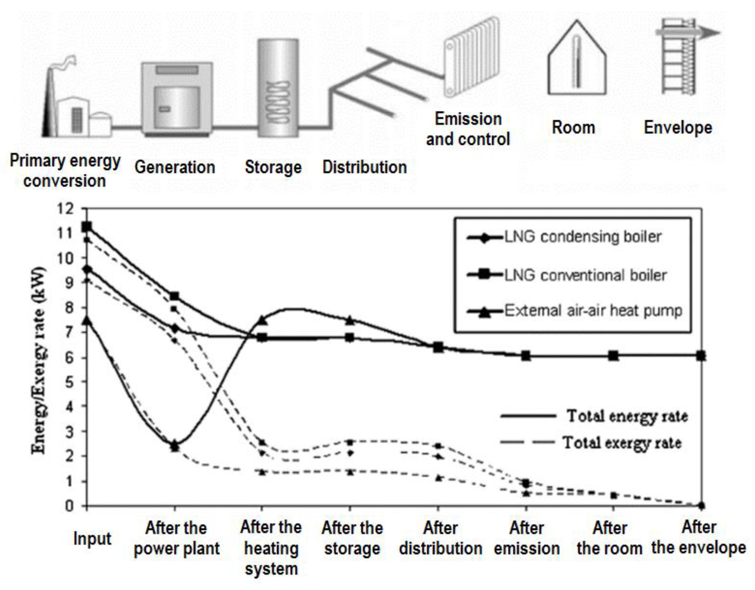
As an example, Yildiz and Gungor considered an office building heated by three possible different systems (i.e., a conventional gas boiler, a condensing gas boiler, and an air-to-air heat pump) [19]. In their study, they calculated the energy and exergy flows through all the components, from the source (primary energy depletion) to the sink (heat losses from the building envelope to the environment). Indoor and outdoor air temperatures were set to be constant at 20 °C and 0 °C, respectively.
From the plots reported in 
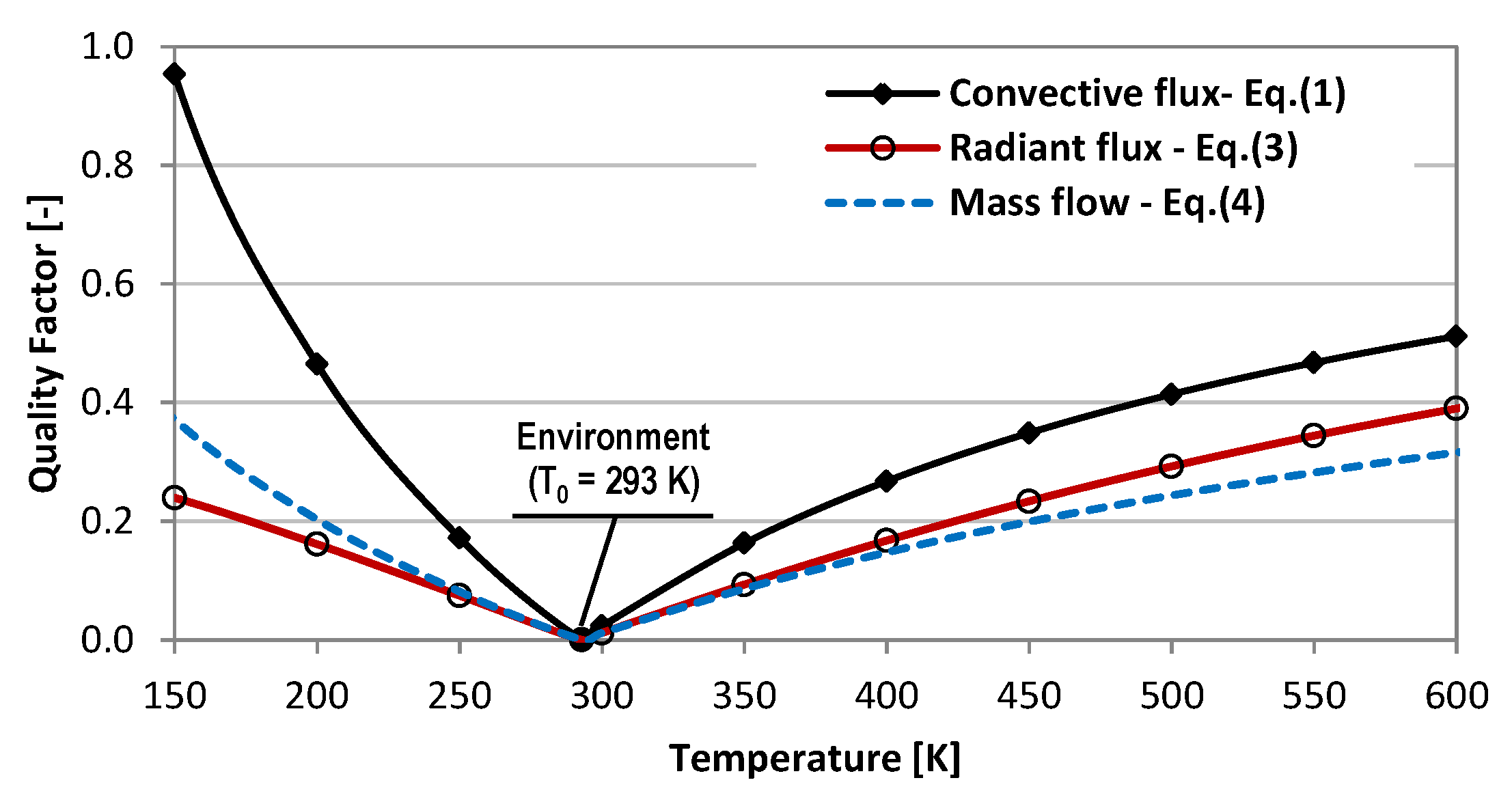
Figure 3, it is possible to observe that the thermal power delivered from the emission system to the room, and then transferred from the room to the outdoor environment, is around 6 kW. The exergy attributed to the heat released by the emission system is not the same for all the heating systems. Indeed, gas boilers are coupled to radiators (inlet and outlet water temperatures of 90 and 70 °C and 70 and 55 °C for conventional and condensing boilers, respectively); on the other hand, purely convective terminals (fan-coils), releasing air at 35 °C, are used with the air-to-air heat pump, which is the case with the lowest exergy content.
In any case, the thermal power delivered to the room has very low exergy content when made available at the indoor temperature (the quality factor being around 7%); the thermal energy leaving the building to the environment has no potential to produce useful work (zero exergy content), whatever the energy conversion system used for space heating. Overall, the largest exergy input pertains to the conventional gas boiler (ηE = 3.8%), whereas the heating system with the heat pump has the best exergy performance (ηE = 5.5%).
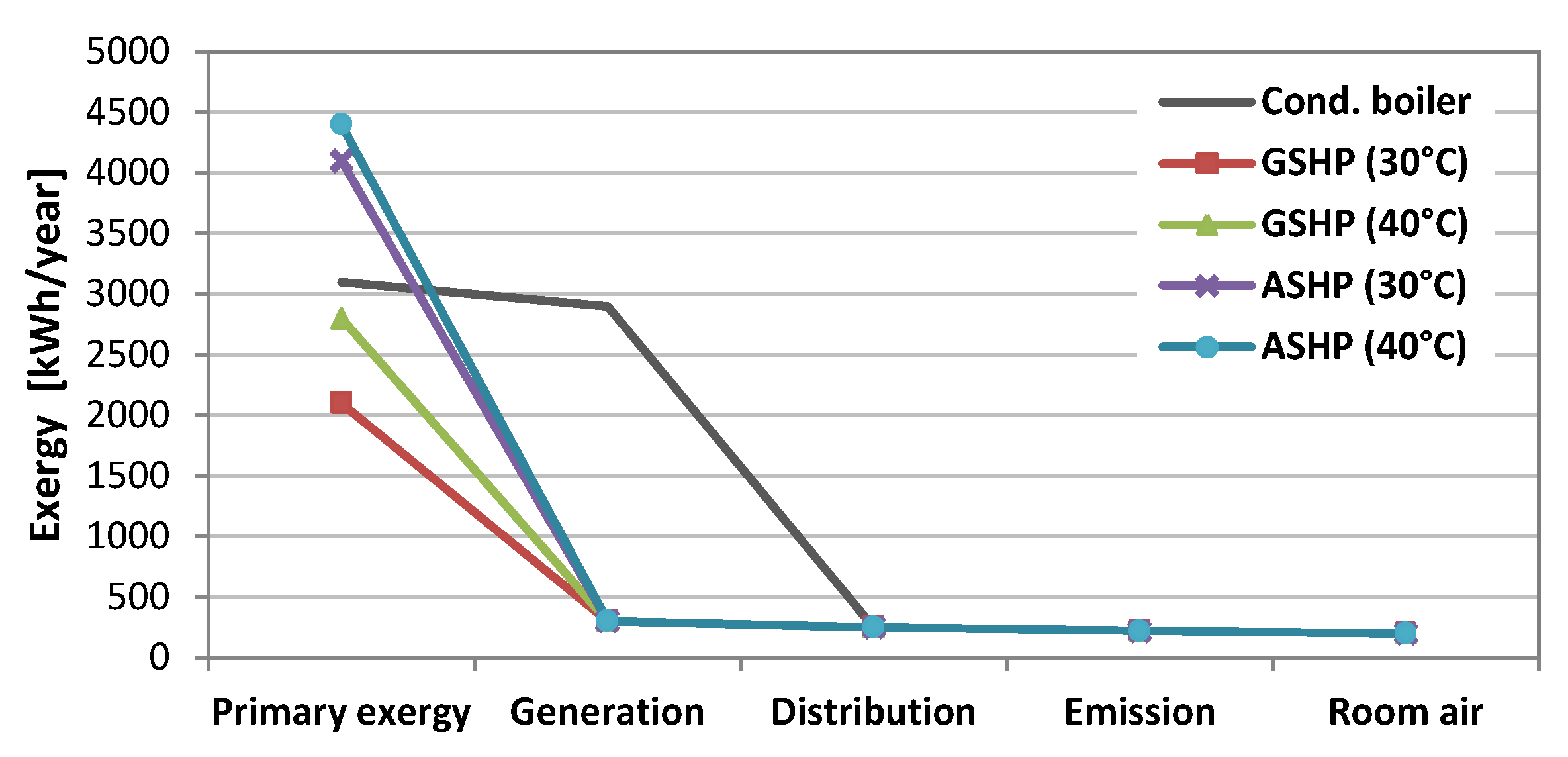
Similar results are obtained by Lohani [20], who studied the energy and exergy flows in a space heating system for a fictitious single-zone building, simulated through the commercial software tool IDA-ICE. In this case, the emission system is a radiant floor fed by hot water at a maximum inlet temperature of 40 °C, while the indoor air temperature oscillates between 21 °C and 23 °C. In the study, Lohani considered a base case where the hot water for the radiant floor is produced by a condensing boiler, plus a series of variants exhibiting air source heat pumps (ASHP) and ground source heat pumps (GSHP) operating at two different condensation temperatures (30 °C and 40 °C). The ground temperature for the ground-source heat pump was set to be constant at 8 °C.
In this study, two different reference temperatures were considered, namely the undisturbed ground temperature (8 °C) and the time-varying outdoor air temperature. The results reported in Figure 4 refer to the second case, and show that the GSHP exploits the lowest exergy amongst the proposed systems, especially if operated at the lowest condensing temperature (30 °C). The overall exergy efficiency turns out to be in the range between 3.5% (ASHP = 40 °C) and 7.1% (ASHP = 30 °C); however, these values are even smaller if the ground temperature is held as the dead state for exergy calculation.
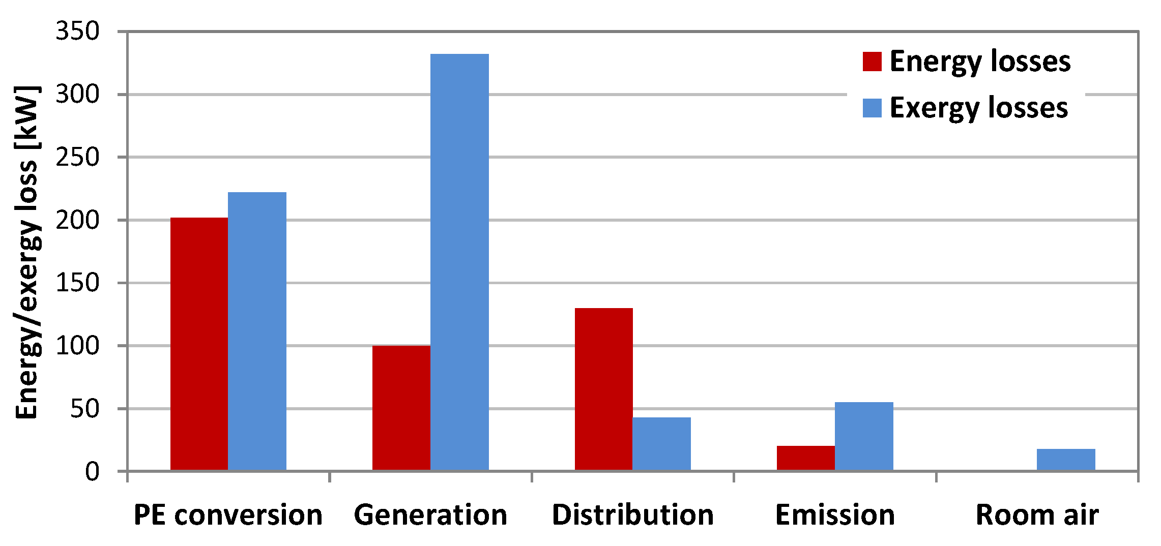
Furthermore, Yucer and Hepbasli performed the exergy analysis of an educational building with a diesel boiler and radiators operating at 80 °C; indoor and outdoor air temperatures were set at 20 °C and 0 °C, respectively [21]. In this study, the overall exergy efficiency turned out to be ηE = 2.7%, with very high exergy destruction rates occurring in the generator (Figure 5).
Another example is provided by Zhou and Gong, who studied a six-story residential building with split-type air conditioners for space heating and cooling [22]. They considered possible improvements to the thermal insulation of the envelope and/or potential improvements to the Coefficient of Performance COP of the split units, which gave rise to an increase in the overall annual exergy efficiency from ηE = 5.1% (base case) to ηE = 7.9%. They also highlighted that using hourly outdoor temperature values for the dead state, in place of a constant reference temperature (corresponding to the average outdoor temperature), would lead to significantly different results; indeed, the discrepancy would range from 9% (heating season) to 21% (cooling season).
However, Baldo and Leoncini came to slightly different conclusions [23]. In fact, they performed the exergy analysis of a multi-story apartment building with a centralized gas-fueled condensing boiler (heating set point at 20 °C), plus individual electric boilers for DHW production (at 45 °C). Individual split units were also available for space cooling (set point at 26 °C). In their study, the choice of different reference temperatures (hourly or monthly average outdoor temperature) led, in both cases, to the same overall exergy efficiency (ηE = 4.6%). However, choosing the dead state as the yearly average outdoor temperature would yield ηE = 3.4%.
Finally, Gonçalves et al. studied the exergy performance of a four-star hotel located in the city of Coimbra, Portugal [24]. The energy conversion systems installed in the hotel included a centralized gas boiler for space heating (set-point temperature = 20 °C) and DHW (water temperature = 60 °C), and a chiller for space cooling (set-point temperature = 26 °C). Additionally, some individual air conditioning units were installed to work as auxiliaries of the main central system. In their exergy analysis, the authors also included cooking activities, to which they attributed a delivery temperature of 150 °C, and all electricity needs for lighting, appliances, and ventilation.
As far as the dead state is concerned, the authors considered the monthly average outdoor air temperatures for heating, cooling, and cooking application, and a constant dead state temperature of 10 °C for DHW uses (i.e., the minimum water temperature in the distribution network).
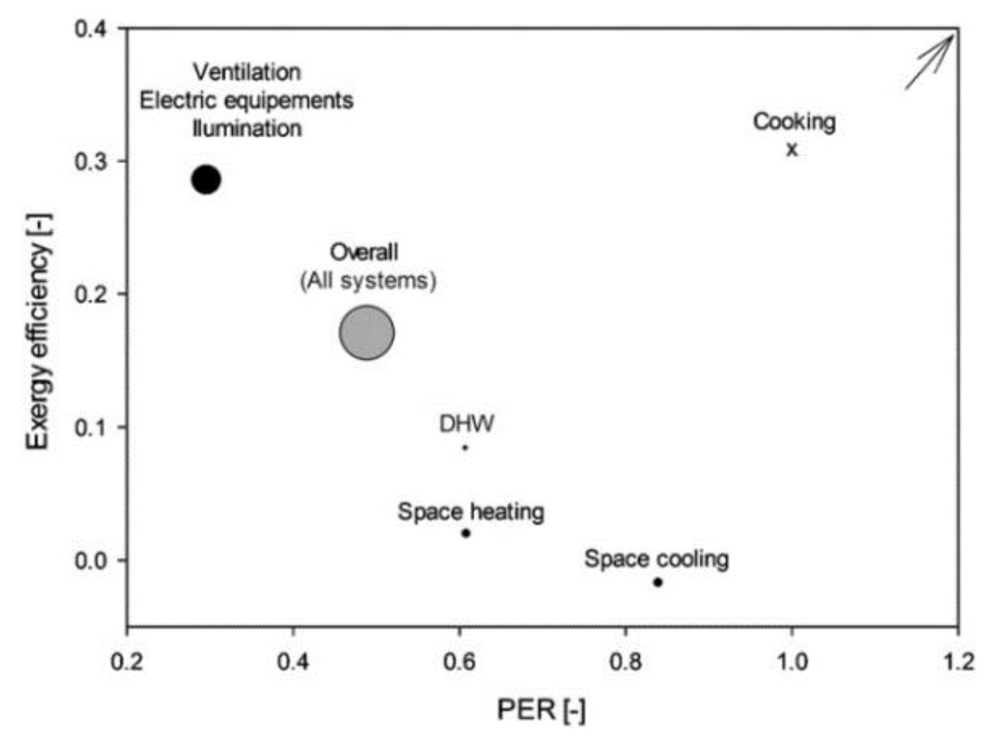
The novelty of this study is that a “map” is proposed to comment the results, where energy and exergy performance can be compared at a glance through the Primary Energy Ratio (PER) and the exergy efficiency, respectively (see Figure 6). The results suggest that electric equipment, lighting, ventilation, and other electric devices show poor energy performance, since they are responsible for high primary energy consumption for unit final energy use (PER ≈ 0.3); however, they show high exergy efficiency (ηE = 28%), meaning that they use energy–and in particular electricity—in a rational way. On the other hand, space heating and cooling reveal higher PER values, but very low exergy efficiency (ηE = 3% for space heating). The best compromise, that is to say high PER values and high exergy efficiency, pertains to cooking activities, which use fuel for high-temperature applications. Overall, the average exergy efficiency for all the energy uses is around 17%.
The important role of the electricity consumption for the auxiliary components in low-exergy heating systems has also been extensively discussed by Kazanci et al. [25]. Their study presents the steady-state exergy analysis of several heating systems for a residential unit in Denmark (radiators, floor heating, air-handling unit), with a constant reference temperature set to T0 = −5 °C. The results underline that the pumps operating in the floor heating system show higher electricity consumption than with common radiators, due to the lower temperature drop and the consequent higher mass flow rate. As a result, additional exergy needs must be computed, which in certain cases may even overcome the advantage of using low-temperature radiant terminals. Similar outcomes are found when dealing with air-handling units; here, there is a trade-off between the exergy gain introduced by a heat recovery unit and the additional electricity consumption due to the higher pressure losses and the additional exhaust fan. As a general rule, water-based systems require lower auxiliary energy use than air-based heating systems.
Now, as highlighted by Teres-Zubiaga et al. in their study about the exergy analysis of a social dwelling in Bilbao [26], the identification of the exergy losses can suggest the directions for further improvement. As an example, starting from the base case with high temperature radiators and a centralized gas boiler for space heating and DHW, the adoption of low-temperature terminals and a collective combined heat and power (CHP) unit can increase the overall exergy efficiency from ηE = 4.4% to ηE = 10%, with the variable outdoor temperature as the dead state.
Based on this principle, Garcia Kerdan et al. developed a comprehensive multi-objective model embedded into the well-known open-source dynamic building energy simulation tool, EnergyPlus [27,
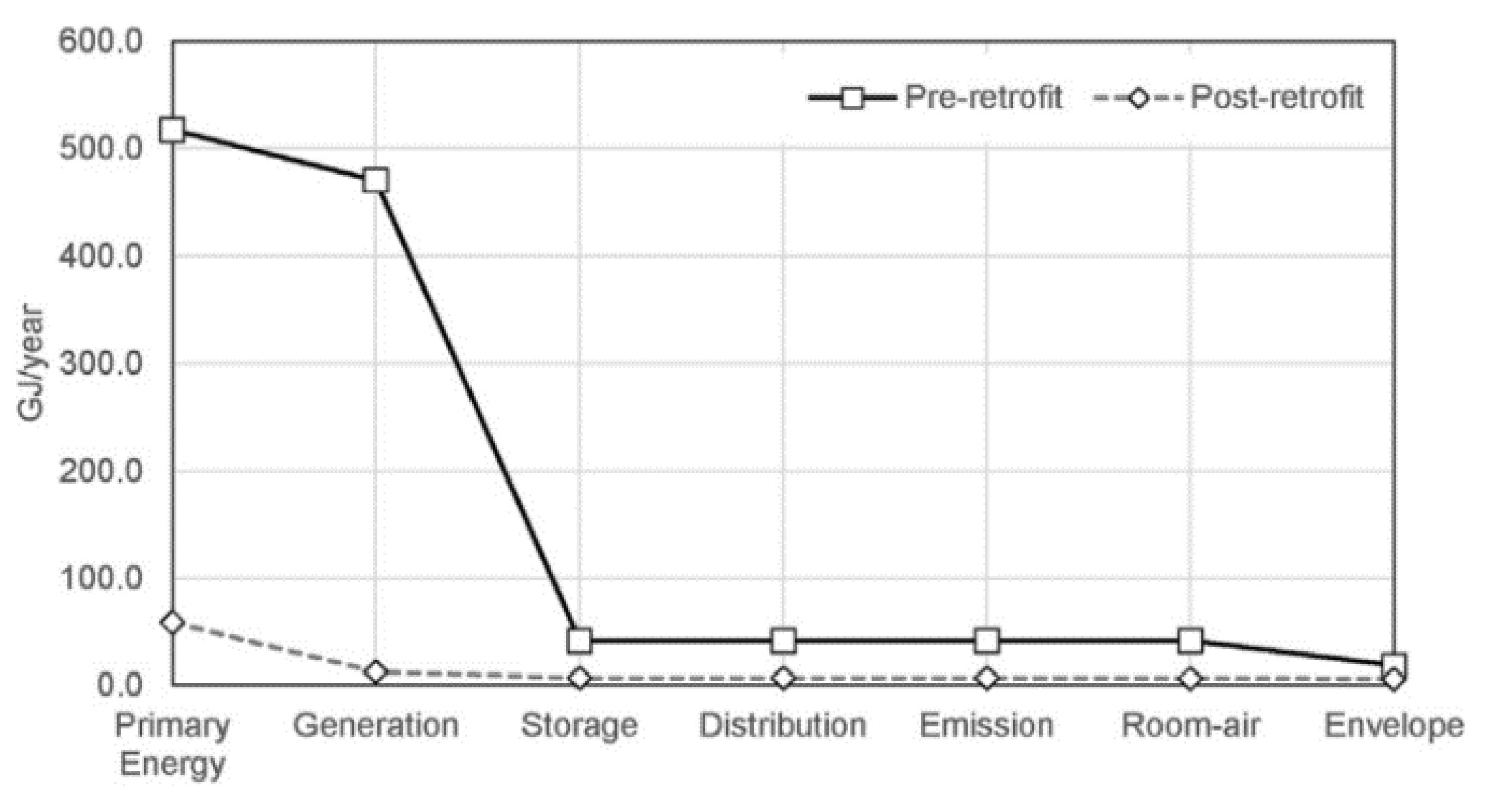
28], with the aim to allow for the exergy optimization of possible retrofit strategies for buildings. This model was applied to the retrofit of a three-story non-domestic Passivhaus in the UK [29]; here space heating and DHW were provided by means of a centralized conventional gas boiler and high temperature radiators. The retrofit solution included the installation of a GSHP unit and medium temperature radiators, as well as a mechanical ventilation system with a 90% efficient heat-recovery unit. Figure 7 illustrates the exergy flows through the energy supply chain of the heating system for both system configurations (before and after retrofit). As one can observe, an important reduction in the primary exergy input is accomplished, making the exergy efficiency increase from ηE = 3.7% to ηE = 10.4%.
Other authors also proposed predictive control strategies to minimize exergy destruction in HVAC systems, and implemented them in control and management systems for a three-story building equipped with a GSHP to provide heating and cooling [30]. If compared to a traditional on–off controller, the proposed exergy-based predictive controller reduces exergy destruction and energy consumption by up to 22% and 36%, respectively.

3.2. Exergy Analysis of Heat Pump Systems

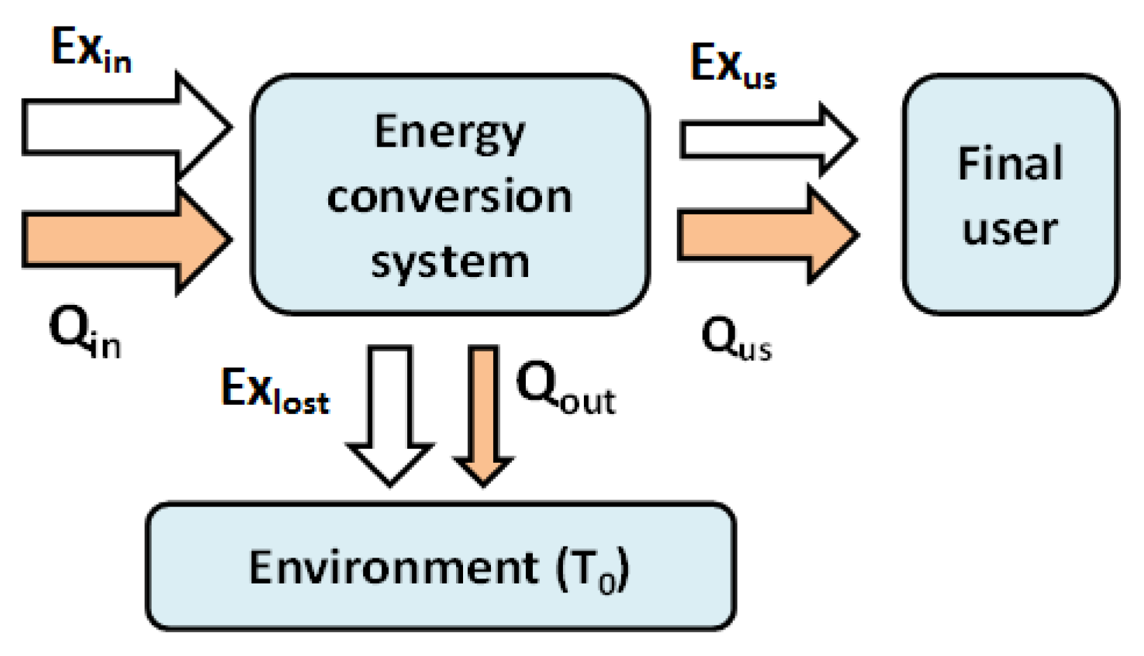
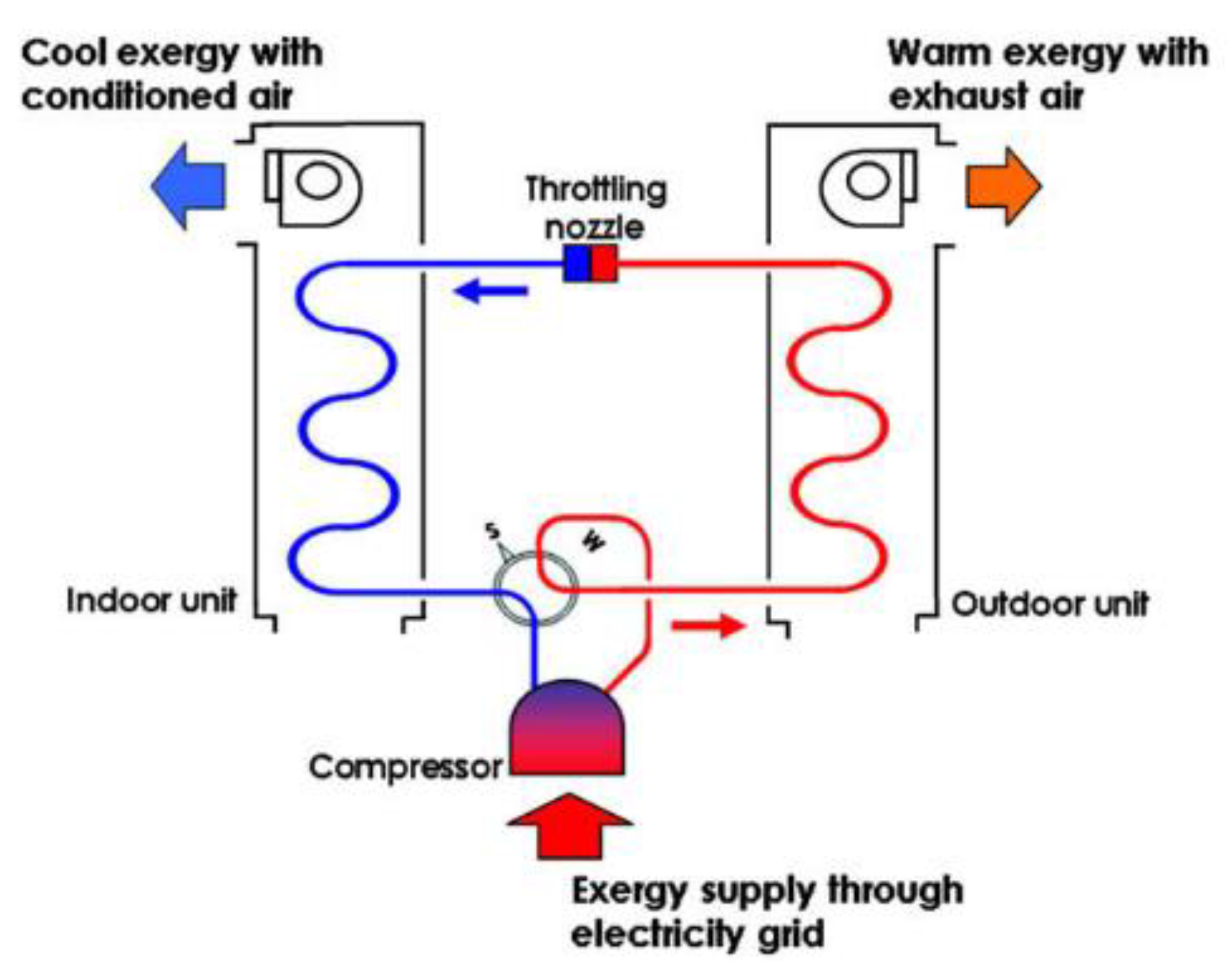
Amongst the different low-energy systems available for building heating and cooling applications, heat pumps show very high potential to behave as a low-exergy system. According to Shukuya [31], common air-source heat pumps used in buildings can be regarded as devices that need a certain amount of exergy in the form of electricity, and then provide a portion of it to the indoors as cool or warm exergy according to the seasonal use (see Figure 8). Typical exergy efficiency values for reversible air-source heat pumps, in buildings application, range between 12% and 15%.
Interestingly, Shukuya also introduced the concept of “wet” and “dry” exergy in analogy to that of “cool” and “warm” exergy, which is particularly relevant when dealing with air-conditioning systems aimed to control the indoor humidity level [2]. In fact, wet exergy is defined as the ability of a volume of air with a given amount of water vapor to disperse into an environment with less humid air; conversely, dry exergy is defined as the ability of the water vapor contained in the outdoor environment to disperse into a volume with lower water vapor content. However, these concepts were not used in any of the reviewed papers concerning the application of heat pumps in buildings.
In relation to the chilled water circuit of a reversible heat pump system, Yin et al. [32] analyzed the effects of different variable-flow control strategies (throttle valve, constant pressure, constant differential pressure, and predictive system curve) and different supply water temperatures (7 °C and 12 °C, respectively) on the input (Exin) and useful (Exus) exergy flows. The results show that a higher supply water temperature and the adoption of a predictive system curve control can reduce exergy consumption (Exlost) by around 60%, thus increasing the exergy efficiency up to about 30%.
Kazanci et al. [33] also demonstrated that coupling a radiant floor cooling system to a ground heat exchanger is a very effective strategy, since the exergy supply from the ground matches well with the low exergy demand of the floor cooling system. In particular, it is possible to reduce the exergy input to the power plant by 90%.
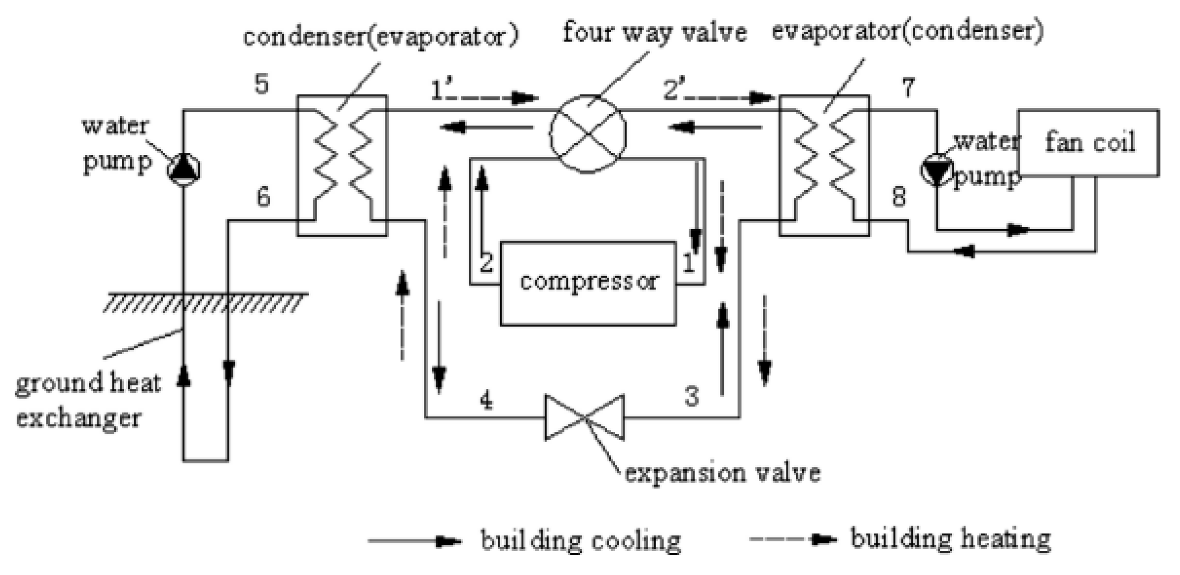
A rather high number of papers deal with the exergy analysis of ground source heat pumps (GSHPs). In a pioneering work, Bi et al. [34] presented the exergy analysis of a GSHP system in a holiday hotel in Beijing, for both heating and cooling modes (see Figure 9). Here, the authors employed five complementary exergy indices:
  • The exergy consumption (Exlost), both at single component level and at system level;
  • The exergy efficiency, both at single component level and at system level;
  • The exergy loss ratio, defined as the ratio of the exergy losses in the single component to those in the whole system;
  • The exergy loss coefficient, defined as the ratio of the exergy losses in the single component to the amount of exergy incoming to the whole system Exin;
  • Thermodynamic perfect degree, defined as (Exin + Exlost)/Exus for both the single components and the system as a whole.
The study underlines that these indices should be used altogether, because they depict exergy flows under different scales (component or system) and perspectives (input, output, and consumption). Further, specific care should be given to the reduction of exergy losses in the compressor (i.e., the component with the highest exergy loss ratio) and to the optimization of the ground heat exchanger (i.e., the component with the lowest exergy efficiency and thermodynamic perfect degree). Overall, the GSHP system showed reasonable values of exergy efficiency (ηE = 10% in the heating mode and ηE = 7% in the cooling mode).
Similarly, Hu et al. investigated five different control strategies, with the aim of improving the annual exergy efficiency and coefficient of performance (COP) of a GSHP used in a public building in Wuhan (China), while also reducing exergy losses and energy consumption [35]. The authors adopted a dynamic approach, both for building thermal loads and for system operation calculations, and used the hourly outdoor dry bulb temperature as the reference state. The results show that the overall exergy efficiency can rise from 9.0% to 10.4% in the heating mode, and from 6.1% to 6.9% in the cooling mode, thanks to the use of variable speed pumps for flow rate control. For this scenario, COP values in heating and cooling modes can reach seasonal values as high as 3.8 and 3.7, respectively, which is a noticeable improvement if compared to the starting values of 2.7 and 3.2, respectively.
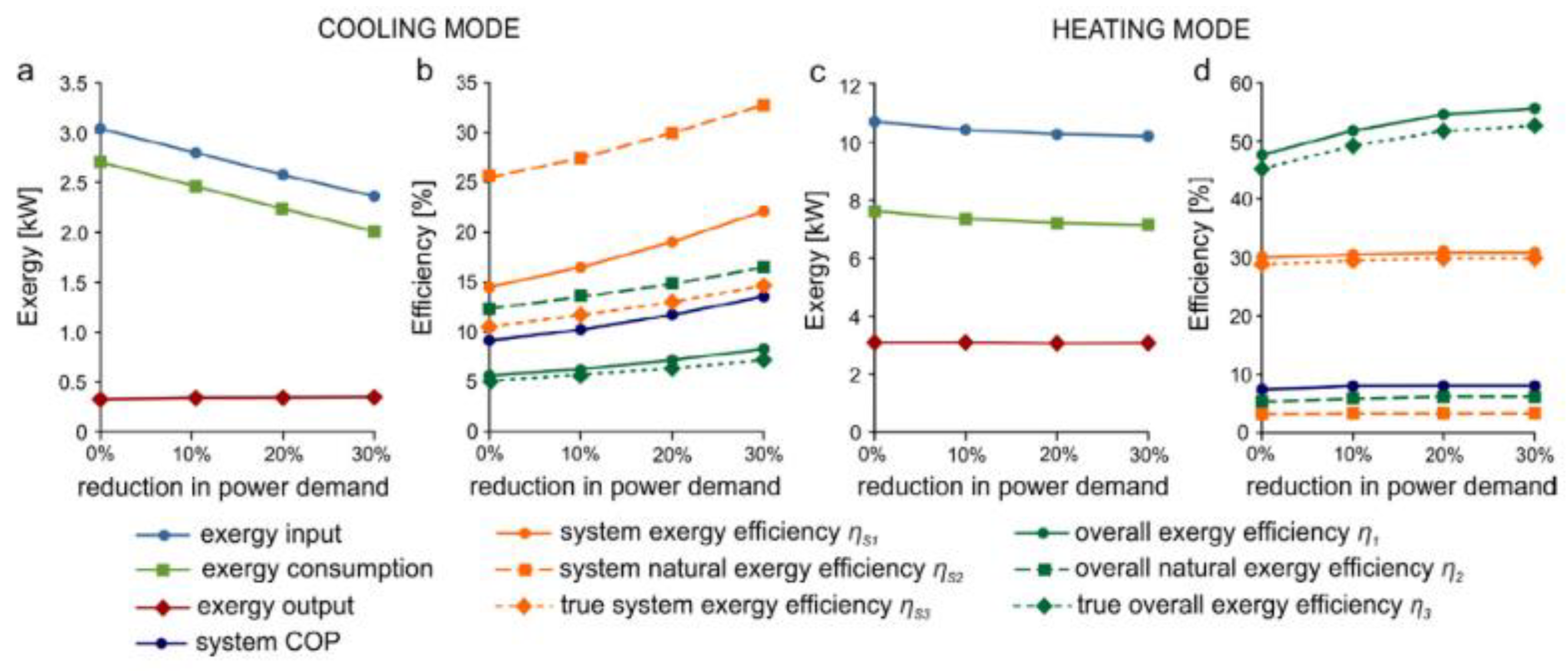
Furthermore, different scenarios for improving the operational efficiency of a GSHP system equipped with a supplementary gas-fired boiler were investigated by Menberg et al., taking the Architecture studio building of the Cambridge University (UK) as a case study [36]. After developing a comprehensive mathematical formulation for each component of the system under steady-state conditions, with fixed temperatures for the outdoor and indoor environments, the heating and cooling performance was analyzed by means of six performance indicators. The dead state temperature is constant and corresponds to the design outdoor temperatures (i.e., 0 °C in winter and 30 °C in summer).
The main novelties of this work reside in the consideration of chemical exergy for the use of natural gas, and in the definition of the natural exergy ratio (i.e., the share of the natural exergy input (from natural gas) in the total exergy input from all sources). The results reveal that the highest exergy losses occur in the heat exchanger between the heating loop and the gas-fired boiler, with a share of approximately 50% of the total exergy losses in the heating mode. The overall exergy input in the cooling mode is significantly lower, but the exergy delivered to the user is also low, mainly because the design indoor temperature in summer is very close to the reference temperature. Moreover, a potential reduction in the electricity consumption of pumps and fans, based on the possibility of replacing them with highly efficient auxiliary components, revealed a potential increase from 6.0% to 7.5% in the cooling mode and from 47.3% to around 55.0% in the heating mode (as shown by the so called “true overall exergy efficiency” in Figure 10).
Finally, Tolga Balta et al. [37] applied a steady-state approach to study the exergy performance of a real GSHP used for space heating and cooling in a test room located in the Aksaray University (Turkey). In their study, indoor and outdoor air temperatures are 20 °C and −15 °C, respectively, while the heat pump operates with a maximum supply temperature of 55 °C. The current outdoor temperature defines the dead state. Again, the highest exergy destruction pertains to the primary energy transformation process and to the ground heat exchanger; the overall exergy efficiency is ηE = 4.9%.

3.3. Exergy Analysis of Solar Systems in Buldings

Although many studies refer to the exergy optimization of different solar systems—especially PV, PV with heat recovery and absorption heat pumps, as in [38]—only a few papers deal with their integration with buildings. Among them, those by Meggers et al. [39] and by Koroneos and Tsarouhis [40] are worth citing, as they concern the combined use of PVT and GSHP systems.
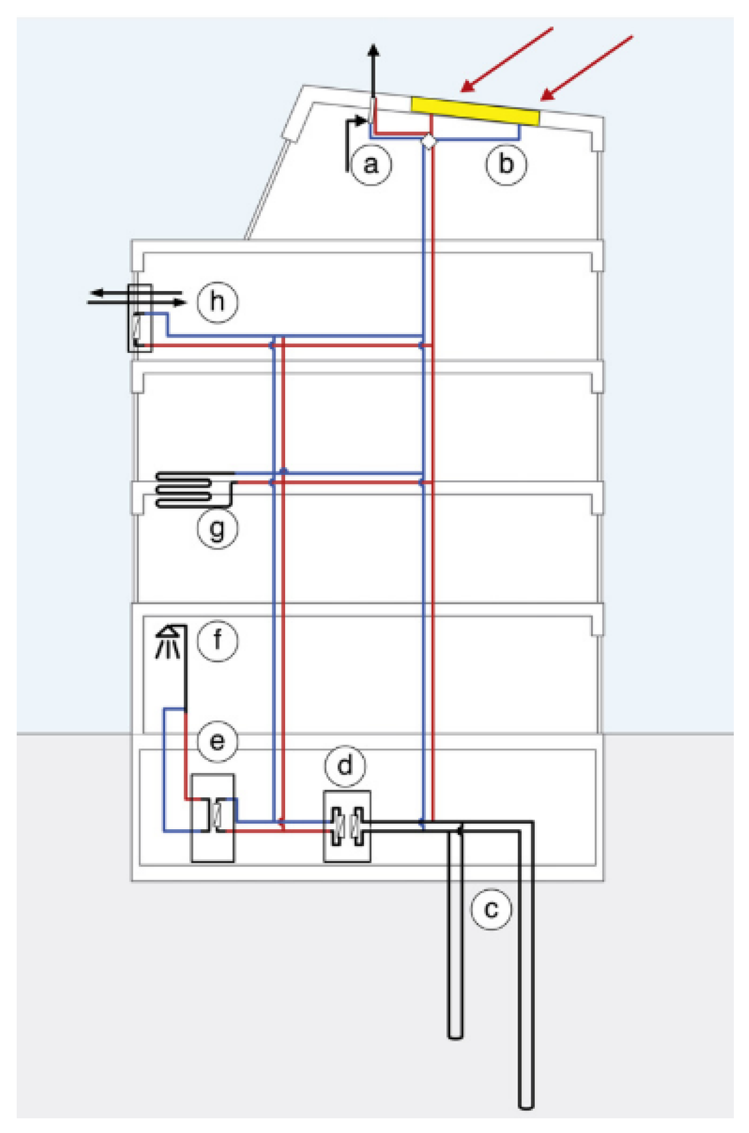
In [39], the authors reported on the updates concerning the integration of several low-exergy systems employed in the framework of the B35 project in Zurich (Switzerland). More in detail, heating and cooling are provided via a GSHP connected with a dual zone borehole of 150 m and 380 m length, respectively. A PVT system on the roof is instead used for either supplying hot water to the heat pump for DHW production or for regenerating the boreholes section (see Figure 11 for the schematic of the integrated system).
The results from both the experimental campaign and the dynamic thermal simulations with TRNSYS showed that, by limiting the temperature lift in the heat pump to less than 20 °C, average performance factors up to COP = 8 can be obtained throughout the year. Furthermore, in this configuration the PVT panels can achieve a thermal efficiency of around 40% and an electrical efficiency ranging between 12% and 14%.
However, the above paper does not present any calculation concerning exergy, whereas in [40] the exergy analysis is coupled with life cycle assessment (LCA) to investigate the performance of solar heating, cooling, and DHW systems employed in a detached house in Thessaloniki (Greece). Concerning PVT’s exergy performance, exergy efficiency in the range of 5% for space heating, 9% for space cooling, and 7% for DHW production is found. No explicit reference is made to the choice of the dead state conditions used for calculation purposes.
A building integrated photovoltaic thermal (BIPVT) system was the object of the study from Agathokleous et al. [41]. Here the authors analyzed, in detail, a naturally ventilated BIPVT system applied to a test rig facing east and located in Limassol (Cyprus), with the aim of determining the energy and exergy efficiencies of the system under varying outdoor conditions (namely solar radiation and dry bulb temperature). Exergy calculations, carried out assuming a dead state temperature equal to the hourly outdoor air temperature and a fixed wall temperature of 26 °C, revealed that an air gap of 10 cm is sufficient to avoid overheating for the PV panels; indeed, the highest PV temperature observed experimentally is 57 °C. The resulting overall energy and exergy efficiencies range between 26.5% and 33.5%, and 13% from 16%, respectively, depending not only on the climate variables but also on the temperature of the fluid at the outlet (i.e., the higher the temperature the better the efficiencies).
Additionally, Gupta et al. [42] studied a semi-transparent BIPVT system applied to a sloped roof surface in Varanasi (India), with potential applications in the fields of solar drying, crop cultivation, and sun bathing. The authors made an attempt to comprehensively consider the electrical, thermal, and daylighting efficiencies of the system under varying outdoor temperatures and solar radiation conditions. However, the exergy calculation for daylight provision is based on rough assumptions (e.g., a fixed conversion rate from solar radiation to visible light (1 W = 100 lx)), which neglects the human eye’s sensitivity to different wavelengths. Nevertheless, the values for electrical, daylighting, and thermal exergy efficiency are found to be around 10%, 11%, and 23%, in order, irrespective of the different ventilation rates assumed in the room below the BIPVT system.
Another noticeable example of integrated solar systems to provide heating, cooling, and DHW to a dwelling can be found in [43], where a novel LiCl-H2O thermally-driven heat pump is coupled with solar thermal collectors and with an outdoor pool acting as a heat sink. The water in the pool is maintained at a comfortable temperature of 24 °C, and this makes it possible to extend the swimming period and to increase the exergy efficiency, thanks to the lower exergy destructions. More in detail, the dynamic simulations of a single-family house carried out with TRNSYS for the cities of Leon, Madrid, and Seville, in Spain, revealed how the integration of these solar systems can lead to an overall exergy efficiency value—calculated dynamically as a function of the outdoor air temperature—up to 28%. This figure can drop down to around 14% for certain values of the heating to cooling ratio of the building (i.e., according to local climate conditions).
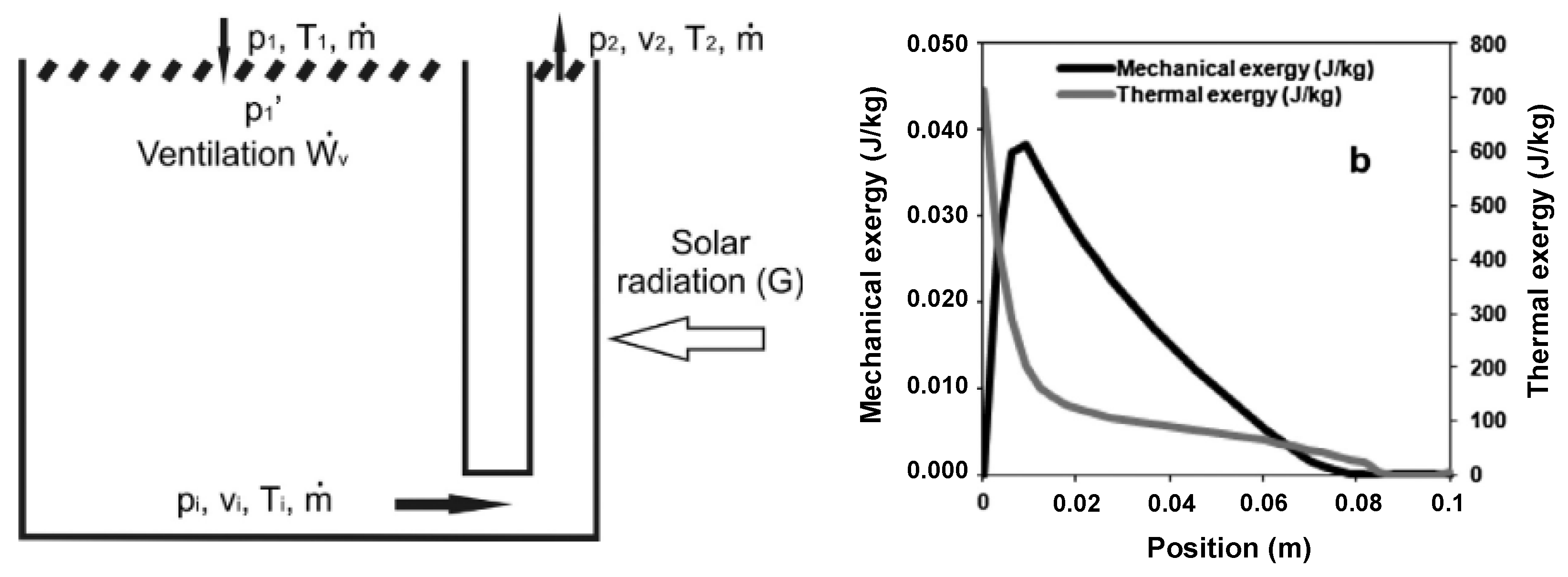
Finally, a paper by Suárez-López et al. [44] is worth mentioning. Here, thermal and mechanical exergy efficiencies are calculated for a solar chimney device used for passive cooling purposes (see Figure 12). By developing a three-dimensional Computational Fluid Dynamics (CFD) model of a rectangular solar chimney, and by considering fixed dead state conditions (T0 = 30 °C, p0 = 1.013 bar, z0 = 0 m), exergy efficiency figures are calculated at the inlet and the outlet of the chimney channel for different values of the solar irradiance. Thermal and total exergy efficiencies result almost identical and equal to 0.55%; actually, this very low value is reasonable if one considers the very small temperature increase in the chimney. Furthermore, mechanical exergy efficiency is very low (i.e., an order of magnitude lower than thermal exergy) because of the low air velocity values achieved within the ventilation channel.

3.4. Exergy Analysis at District or City Scale

Other papers focus on the exergy analysis of buildings and heating systems at a district level, which is the topic currently addressed by ECBCS Annex 64.
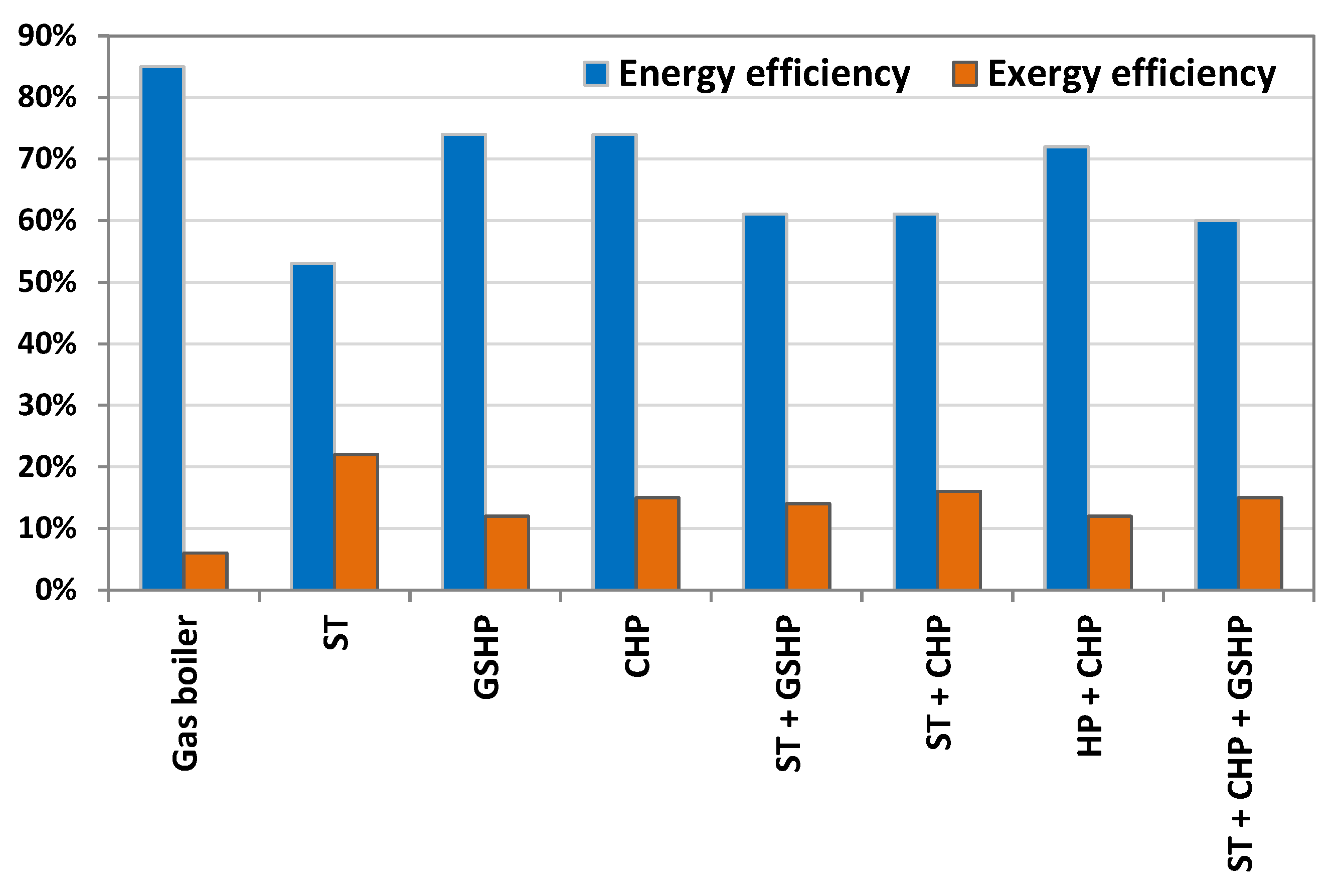
As an example, Kallert et al. [45] modeled ten high-performing residential buildings, heated by a local district heating network, where heat generation was based on different potential combinations of solar thermal collectors, ground source heat pumps, and gas-fired combined heat and power units (CHP). The results show that a suitable combination of these technologies can increase the exergy efficiency up to 15%, or even 22% in the best case (Figure 13).
On the other hand, Kilkis [46] investigated several solutions to minimize exergy waste in a University campus in Sweden, including district heating at low supply temperature, large-scale aquifer thermal energy storage (ATES), heat supply from solar collectors, and photovoltaic/thermal systems (PVT); CHP and PVT units turned out to show the best energy quality. Based on a reference environmental temperature of T0 = 8 °C, suitable combinations of the above mentioned technologies can lead to very high exergy efficiency, ranging from 49% to 81%. On these bases, the same author defined the concept of a net-zero exergy district (NZEXD) (i.e., a district that produces as much energy, at the same grade or quality, as is consumed on an annual basis) [47].
Saeb Gilani et al. considered a district in Berlin comprising ninety-three residential buildings [48], and introduced a fictitious district heating network with four different temperature levels available. In particular, the available nominal supply and return water temperatures are 90 and 70 °C, 70 and 60 °C, and 60 and 45 °C, respectively, which are suitable for the apartments with radiators, and 35 and 28 °C, respectively, for the apartments where floor heating systems are installed. The results showed that a suitable exploitation of this fictitious district heating network has the potential to cut, by 35%, the exergy losses, if compared to a scenario where all apartments are heated by means of hot water at the highest temperature level. Sartor and Dewallef confirmed that the highest exergy efficiency in the heating season can be obtained through a district heating network, feeding a floor radiant heating system operated at low temperature, followed by heat pumps [49].
Another contribution refers to a simulated office building equipped with low-temperature heating and high-temperature cooling systems located in the Netherlands [50]. Here, the authors highlighted that the exergy efficiency can be as low as 3.3%, when burning fossil fuels, to supply thermal energy at 60 °C, whereas supplying thermal energy at 35 °C from district heating can increase the overall exergy efficiency up to ηE = 17.1%. In case of space cooling with chilled water at 10 °C, produced by an electric chiller, the overall exergy efficiency is below 7%.
On the other hand, Yazici investigated the exergy performance of the geothermal district heating network in the Afyon province of Turkey, which includes 17 heat exchangers and 13 pumps, renovated from 2011 to 2013 [51]. The study revealed that the exergy destruction was mainly due to the water re-injected in the aquifer and to the losses in the heat exchanger, the pumps, and the pipeline. Based on a dead state set at T0 = 0.1 °C, the overall exergy efficiency of the network turned out to be ηE = 60.6%, which is in line with the outcomes of the other five studies addressing other geothermal district heating networks in Turkey.
Finally, Causone et al. calculated the overall energy and exergy efficiency at a city scale in Milan, and showed the usefulness of exergy as an indicator for policy makers to compare the potential of different smart urban policies [52]. The best scenario considered in the paper contemplates that half of the total thermal energy use for buildings’ heating is covered through district heating systems, whereas the remaining half is assigned to natural gas; in this case, the overall exergy efficiency approaches 20%. The authors then underline that, in order to explore future decarbonization scenarios, and for effective policymaking, even the building stock at a national level should be studied using exergy analysis, since exergy represents the real value of an energy source.
In this direction, Garcia Kerdan et al. explored seven different large-scale, future retrofit scenarios for the non-domestic building sector in the UK, including typical, low-carbon, and low-exergy approaches [53]. The outcomes show that current regulations can potentially reduce carbon emissions by up to 49.0 ± 2.9% by 2050, while also increasing the thermodynamic efficiency of the whole sector from 10.7% to 13.7%. However, a low-exergy oriented scenario based on renewable electricity and heat pumps would even reduce carbon emissions by 88.2 ± 2.4%, and would achieve a sectorial exergy efficiency of 19.8%.

4. Conclusions

This paper presented a literature review about the exergy analysis of energy conversion systems typically used in buildings for the control of indoor conditions. The review revealed that the vast majority of technologies used for space heating and cooling in buildings shows very poor performance in terms of exergy (i.e., make a very irrational use of the energy sources). Hence, it is important to include the perspective provided by the second law of thermodynamics. Indeed, this adds information to a common energy-based investigation, and makes it possible to address potential improvements and more suitable technologies.
Amongst the main findings of this review, it is possible to learn the following lessons about the design of space heating and cooling systems in buildings:
  • The cooling and heating demand of the building must be minimized from the beginning to achieve reasonable exergy efficiency. Indeed, this would allow the use of more efficient terminals units (e.g., radiant floors) and a broad range of heat sources and sinks;
  • Low-temperature heating and high-temperature cooling systems should be preferred, such as radiant ceilings and radiant floors. Indeed, the fact that heat is transferred mainly through radiant heat exchange further reduces exergy degradation in comparison with convective emission systems;
  • Low-exergy sources should be used for space heating and cooling applications in buildings, such as solar thermal energy, geothermal heat, or low-to-medium temperature waste heat, and their integration should be promoted;
  • Combustion processes are not a rational way to produce low temperature heat. Even condensing boilers, whose energy efficiency is very high, are responsible for the degradation of the high exergy content in natural gas;
  • Electricity is pure exergy, hence electricity consumption for auxiliary components such as pumps and fans should be minimized; for the same reason, electricity production from renewable sources should be promoted (e.g., through PV and PVT systems, or small wind turbines);
  • In well-insulated buildings, the energy needs for DHW cover a significant share of the overall energy bill; in addition, DHW is prepared at a higher temperature than for radiant emission systems, which makes this item responsible for a relatively high exergy degradation rate;
  • Cascading principles should be integrated in the building design, meaning that those appliances needing higher exergy levels (e.g., DHW) must be served prior to the appliances with lower exergy content (e.g., radiant heating systems), thus making a rational use of energy;
  • Districts and cities should implement exergy analysis when planning their route to an efficient use of energy.
However, one major shortcoming emerging from the literature is the lack of consensus around the definition of a clear, unambiguous, and scientifically sound dead state condition (also called reference state). In fact, despite a common agreement being found on the choice of the outdoor air as the heat sink for space heating and cooling processes in buildings, researchers dealing with exergy analysis of space heating and cooling systems have, by now, chosen arbitrary (fixed or varying) temperature values. This ambiguity makes impossible to compare, meaningfully, the results of different studies related to the same technology; moreover, it also potentially introduces a series of thermodynamic contradictions that make the study itself not scientifically rigorous.
Actually, this issue is one of the main reasons for the harsh criticism that exergy analysis encounters in the scientific community from many researchers, who disapprove the lack of a commonly accepted methodological framework. Hence, the scientific community should work on an official, shared, and scientifically sound definition of dead state, to be implemented in official texts such as international standards.
The review has also highlighted that a good knowledge about the exergy analysis of space heating and cooling systems is now available, which allows the potential to address the design of these systems under a thermodynamically sound perspective. Future research should be focused on the development on exergy-based control algorithms; these should allow optimum operation and management of low-exergy systems and buildings in order to minimize the exergy destruction, and also in relation to the dynamic variations of the outdoor conditions.

Author Contributions

The work presented in this article is a collaborative development by all the authors.

Funding

The research described in this paper was carried out within the project “Research for SEAP: A platform for municipalities taking part in the Covenant of Mayors”, financed by the Italian Government in the framework of PRIN 2015.

Conflicts of Interest

The authors declare no conflict of interest.

Nomenclature

Variables
ASurface area (m2)
CpSpecific heat at constant pressure (J kg−1 K−1)
ExExergy (J)
hSpecific enthalpy (J kg−1)
IsSolar irradiance (W m−2)
Mass flow rate (kg s−1)
PEPrimary Energy (J)
PEFPrimary Energy Factor (-)
PERPrimary Energy Ratio (-)
QHeat (J)
sSpecific entropy (J kg−1 K−1)
TTemperature (K)
Greek letters
εThermal emissivity (-)
ΣExergy expenditure figure (-)
ηEExergy efficiency (-)
ηQEnergy efficiency (-)
σStefan-Boltzmann constant (5.67 × 10⁻⁸ W m−2 K−4)
ψQuality factor (-)
ΩERate of exergy destruction (-)
Subscripts
inIngoing
lostLost
oEnvironment conditions
outOutgoing
usUseful

References

  1. Schmidt, D. Low Exergy Systems for High-Performance Buildings and Communities. ECBCS Annex 49 Final Report. 2011. Available online: https://www.annex49.info/background.html (accessed on 14 October 2018).
  2. Shukuya, M. Exergy: Theory and Applications in the Built Environment; Springer: London, UK, 2013. [Google Scholar]
  3. Wright, S.E.; Rosen, M.A.; Scott, D.S.; Haddow, J.B. The exergy flux of radiative heat transfer for the special case of blackbody radiation. Exergy 2002, 2, 24–33. [Google Scholar] [CrossRef]
  4. Petela, R. Exergy of undiluted thermal radiation. Sol. Energy 2003, 74, 469–488. [Google Scholar] [CrossRef]
  5. Candau, Y. On the exergy of radiation. Sol. Energy 2003, 75, 241–247. [Google Scholar] [CrossRef]
  6. Jeter, S.M. Maximum conversion efficiency for the utilization of direct solar radiation. Sol. Energy 1981, 26, 231–236. [Google Scholar] [CrossRef]
  7. Pons, M. Exergy analysis of solar collectors, from incident radiation to dissipation. Renew. Energy 2012, 47, 194–202. [Google Scholar] [CrossRef]
  8. Romero, J.C.; Linares, P. Exergy as a global energy sustainability indicator. A review of the state of the art. Renew. Sustain. Energy Rev. 2014, 33, 427–442. [Google Scholar] [CrossRef]
  9. Pons, M. On the reference state for exergy when ambient temperature fluctuates. Int. J. Thermodyn. 2009, 12, 113–121. [Google Scholar] [CrossRef]
  10. Sangi, R.; Müller, D. Exergy-based approaches for performance evaluation of building energy systems. Sustain. Cities Soc. 2016, 25, 25–32. [Google Scholar] [CrossRef]
  11. Marletta, L. Air conditioning systems from a 2nd Law perspective. Entropy 2010, 12, 859–877. [Google Scholar] [CrossRef]
  12. Tronchin, L.; Fabbri, K. Analysis of buildings’ energy consumption by means of exergy method. Int. J. Exergy 2008, 5, 605. [Google Scholar] [CrossRef]
  13. Evola, G.; Marletta, L. Exergy and thermoeconomic optimization of a water-cooled glazed hybrid photovoltaic/thermal (PVT) collector. Sol. Energy 2014, 107, 12–25. [Google Scholar] [CrossRef]
  14. Sangi, R.; Müller, D. Implementation of a solution to the problem of reference environment in the exergy evaluation of building energy systems. Energy 2018, 149, 830–836. [Google Scholar] [CrossRef]
  15. Choi, W.; Ooka, R.; Shukuya, M. Exergy analysis for unsteady-state heat conduction. Int. J. Heat Mass Transfer 2018, 116, 1124–1142. [Google Scholar] [CrossRef]
  16. Torio, H.; Angelotti, A.; Schmidt, D. Exergy analysis of renewable energy-based climatisation systems for buildings: A critical view. Energy Build. 2009, 41, 248–271. [Google Scholar] [CrossRef]
  17. Angelotti, A.; Caputo, P.; Solaini, G. Steady versus dynamic exergy analysis: The case of an air source heat pump. Int. J. Exergy 2012, 11, 460–472. [Google Scholar] [CrossRef]
  18. Hepbasli, A. Low exergy (LowEx) heating and cooling systems for sustainable buildings and societies. Renew. Sustain. Energy Rev. 2012, 16, 73–104. [Google Scholar] [CrossRef]
  19. Yildiz, A.; Güngör, A. Energy and exergy analyses of space heating in buildings. Appl. Energy 2009, 86, 1939–1948. [Google Scholar] [CrossRef]
  20. Lohani, S.P. Energy and exergy analysis of fossil plant and heat pump building heating system at two different dead-state temperatures. Energy 2010, 35, 3323–3331. [Google Scholar] [CrossRef]
  21. Yucer, C.T.; Hepbasli, A. Thermodynamic analysis of a building using exergy analysis method. Energy Build. 2011, 43, 536–542. [Google Scholar] [CrossRef]
  22. Zhou, Y.; Gong, G. Exergy analysis of the building heating and cooling system from the power plant to the building envelop with hourly variable reference state. Energy Build. 2013, 56, 94–99. [Google Scholar] [CrossRef]
  23. Baldi, M.G.; Leoncini, L. Effect of reference state characteristics on the Thermal Exergy analysis of a building. Energy Procedia 2015, 83, 177–186. [Google Scholar] [CrossRef]
  24. Gonçalves, P.; Gaspar, A.R.; Da Silva, M.G. Energy and exergy-based indicators for the energy performance assessment of a hotel building. Energy Build. 2012, 52, 181–188. [Google Scholar] [CrossRef]
  25. Kazanci, O.B.; Shukuya, M.; Olesen, B.W. Exergy performance of different space heating systems: A theoretical study. Build. Environ. 2016, 99, 119–129. [Google Scholar] [CrossRef] [Green Version]
  26. Terés-Zubiaga, J.; Jansen, S.C.; Luscuere, P.; Sala, J.M. Dynamic exergy analysis of energy systems for a social dwelling and exergy based system improvement. Energy Build. 2013, 64, 359–371. [Google Scholar] [CrossRef]
  27. García Kerdan, I.; Raslan, R.; Ruyssevelt, P.; Morillón Gálvez, D. ExRET-Opt: An automated exergy/exergoeconomic simulation framework for building energy retrofit analysis and design optimisation. Energy 2017, 192, 33–58. [Google Scholar] [CrossRef] [Green Version]
  28. García Kerdan, I.; Raslan, R.; Ruyssevelt, P. An exergy-based multi-objective optimisation model for energy retrofit strategies in non-domestic buildings. Energy 2016, 117, 506–522. [Google Scholar] [CrossRef] [Green Version]
  29. García Kerdan, I.; Raslan, R.; Ruyssevelt, P.; Vaiciulyte, S.; Morillón Gálvez, D. Thermodynamic and exergoeconomic analysis of a non-domestic Passivhaus retrofit. Build. Environ. 2017, 117, 100–117. [Google Scholar] [CrossRef] [Green Version]
  30. Razmara, M.; Maasoumy, M.; Shahbakhti, M.; Robinett, R.D. Optimal exergy control of building HVAC system. Appl. Energy 2015, 156, 555–565. [Google Scholar] [CrossRef]
  31. Shukuya, M. Exergy concept and its application to the built environment. Build. Environ. 2009, 44, 1545–1550. [Google Scholar] [CrossRef]
  32. Yin, H.; Ooka, R.; Shukuya, M. Application of exergy analysis to chilled water circuit and heat pump system. Energy Procedia 2015, 78, 1075–1080. [Google Scholar] [CrossRef]
  33. Kazanci, O.B.; Shukuya, M.; Olesen, B.W. Theoretical analysis of the performance of different cooling strategies with the concept of cool exergy. Build. Environ. 2016, 100, 102–113. [Google Scholar] [CrossRef] [Green Version]
  34. Bi, Y.; Wang, X.; Liu, Y.; Zhang, H.; Chen, L. Comprehensive exergy analysis of a ground-source heat pump system for both building heating and cooling modes. Appl. Energy 2009, 86, 2560–2565. [Google Scholar] [CrossRef]
  35. Hu, P.; Hu, Q.; Lin, Y.; Yang, W.; Xing, L. Energy and exergy analysis of a ground source heat pump system for a public building in Wuhan, China under different control strategies. Energy Build. 2017, 152, 301–312. [Google Scholar] [CrossRef]
  36. Menberg, K.; Heo, Y.; Choi, W.; Ooka, R.; Choudhary, R.; Shukuya, M. Exergy analysis of a hybrid ground-source heat pump system. Appl. Energy 2017, 204, 31–46. [Google Scholar] [CrossRef]
  37. Tolga Balta, M.; Kalinci, Y.; Hepbasli, A. Evaluating a low exergy heating system from the power plant through the heat pump to the building envelope. Energy Build. 2008, 40, 1799–1804. [Google Scholar] [CrossRef]
  38. Marletta, L. Exergy Analysis of Solar Cooling Systems. A Technical Report of Subtask C3 of IEA SHC Task 38. 2010. Available online: https://task38.iea-shc.org/publications (accessed on 19 October 2018).
  39. Meggers, F.; Ritter, V.; Goffin, P.; Baetschmann, M.; Leibundgut, H. Low exergy building systems implementation. Energy 2012, 41, 48–55. [Google Scholar] [CrossRef]
  40. Koroneos, C.; Tsarouhis, M. Exergy analysis and life cycle assessment of solar heating and cooling systems in the building environment. J. Clean. Prod. 2012, 32, 52–60. [Google Scholar] [CrossRef]
  41. Agathokleous, R.A.; Kalogirou, S.A.; Karellas, S. Exergy analysis of a naturally ventilated Building Integrated Photovoltaic/Thermal (BIPV/T) system. Renew. Energy 2018, 128, 541–552. [Google Scholar] [CrossRef]
  42. Gupta, N.; Tiwari, A.; Tiwari, G.N. A thermal model of hybrid cooling systems for building integrated semitransparent photovoltaic thermal system. Sol. Energy 2017, 153, 486–498. [Google Scholar] [CrossRef]
  43. Borge, D.; Colmenar, A.; Castro, M.; Martín, S.; Sancristobal, E. Exergy efficiency analysis in buildings climatized with LiCl-H2O solar cooling systems that use swimming pools as heat sinks. Energy Build. 2011, 43, 3161–3172. [Google Scholar] [CrossRef]
  44. Suárez-López, M.J.; Blanco-Marigorta, A.M.; Gutiérrez-Trashorras, A.J.; Pistono-Favero, J.; Blanco-Marigorta, E. Numerical simulation and exergetic analysis of building ventilation solar chimneys. Energy Convers. Manag. 2015, 96, 1–11. [Google Scholar] [CrossRef]
  45. Kallert, A.; Schmidt, D.; Bläse, T. Exergy-based analysis of renewable multi-generation units for small scale low temperature district heating supply. Energy Procedia 2017, 116, 13–25. [Google Scholar] [CrossRef]
  46. Kılkış, Ş.; Wang, C.; Björk, F.; Martinac, I. Cleaner energy scenarios for building clusters in campus areas based on the Rational Exergy Management Model. J. Clean. Prod. 2017, 155, 72–82. [Google Scholar] [CrossRef]
  47. Kilkiş, Ş. Exergy transition planning for net-zero districts. Energy 2015, 92, 515–531. [Google Scholar] [CrossRef]
  48. Saeb Gilani, B.; Bachmann, M.; Kriegel, M. Evaluation of the temperature regimes of multi-level thermal networks in urban areas through exergy analysis. Energy Procedia 2017, 122, 385–390. [Google Scholar] [CrossRef]
  49. Sartor, K.; Dewallef, P. Exergy analysis applied to performance of buildings in Europe. Energy Build. 2017, 148, 348–354. [Google Scholar] [CrossRef] [Green Version]
  50. Sakulpipatsin, P.; Itard, L.C.M.; van der Kooi, H.J.; Boelman, E.C.; Luscuere, P.G. An exergy application for analysis of buildings and HVAC systems. Energy Build. 2010, 42, 90–99. [Google Scholar] [CrossRef]
  51. Yazici, H. Energy and exergy based evaluation of the renovated Afyon geothermal district heating system. Energy Build. 2016, 127, 794–804. [Google Scholar] [CrossRef]
  52. Causone, F.; Sangalli, A.; Pagliano, L.; Carlucci, S. An Exergy Analysis for Milano Smart City. Energy Procedia 2017, 111, 867–876. [Google Scholar] [CrossRef]
  53. García Kerdan, I.; Raslan, R.; Ruyssevelt, P.; Morillón Gálvez, D. The role of an exergy-based building stock model for exploration of future decarbonisation scenarios and policy making. Energy Policy 2017, 105, 467–483. [Google Scholar] [CrossRef] [Green Version]
Figure 1. Exergy related to a unit thermal power as a function of temperature.
Buildings 08 00180 g001
Figure 2. Energy and exergy flows, to and from an energy conversion system.
Buildings 08 00180 g002
Figure 3. Energy and exergy flow rates through the system components [19].
Buildings 08 00180 g003
Figure 4. Exergy flows through the components for different heat generation systems [20].
Buildings 08 00180 g004
Figure 5. Energy and exergy losses in the single components [21].
Buildings 08 00180 g005
Figure 6. Exergy efficiency versus Primary Energy Ratio (PER) for single end uses in a four-star hotel [24].
Buildings 08 00180 g006
Figure 7. Exergy flows: Comparison before and after retrofit [29].
Buildings 08 00180 g007
Figure 8. Working principle of an electricity-driven heat pump [31].
Buildings 08 00180 g008
Figure 9. Layout of the ground source heat pump (GSHP) system analyzed in [32].
Buildings 08 00180 g009
Figure 10. Exergy figures for heating and cooling modes [36]. (a)Total exergy flows in cooling mode; (b) Exergy efficiency in cooling mode; (c) Total exergy flows in heating mode; (d) Exergy efficiency in heating mode.
Buildings 08 00180 g010
Figure 11. Integration of low-exergy systems in a prototype building in Zurich [39]. (a) Exhaust heat recovery; (b) PV panels with heat recovery; (c) dual zone boreholes; (d) heat pump; (e) low temperature hot water storage; (f) warm wastewater recovery; (g) ceiling panels; and (h) decentralized heat supply.
Buildings 08 00180 g011
Figure 12. Left-hand figure: Schematic of the variables used in the analysis. Right-hand figure: Mechanical and thermal exergy values at the exit section of the solar chimney for various distances from the symmetry plane [44].
Buildings 08 00180 g012
Figure 13. Energy and exergy efficiency for different combinations of heating systems (from [45]): ST = solar thermal collectors; GSHP = ground source heat pump; CHP = combined heat and power units.
Buildings 08 00180 g013

