Rebound Characteristics of Wet-Shotcrete Particle Flow Jet from Wall Based on CFD-DEM

Abstract

This paper aims to reveal the motion law and collision behaviors of shotcrete particle flow jets. A physical model of the jet flow field composed of a nozzle structure and jet area was constructed and meshes with various sizes were used to mesh the nozzle and jet area. With the basic contact parameters and contact model parameters of the particles set, the CFD-DEM-coupling simulation method was adopted to perform the numerical simulation of concrete-particle-flow-jet impingement. The variation laws of the continuous-phase velocity and pressure drop of the shotcrete, coarse-aggregate motion characteristics, and particle collision behavior under the interaction of the continuous and discrete phases were obtained. The results showed that the velocity field and pressure-drop field of the continuous phase had an ideal symmetry in the XY plane in the stable injection stage, the continuous-phase velocity gradually increased inside the nozzle and gradually decreased after entering the jet area, the continuous-phase pressure drop was the maximum at the nozzle inlet, and the pressure value at the nozzle outlet became atmospheric pressure. The central axis of the particle flow jet was displaced by 0.15 m in the negative direction of the Y-axis under the action of gravity, the diffusion angle of the small particles that exited the nozzle and entered the jet area was larger than that of the large particles, and the large-particle jets were more concentrated and easier to spray into the designated spraying areas. The particle flow reached a stable jet state about 0.3 s after the jet began, and the peak velocity of the 4 mm particles in the flow reached 25 m/s, while the peak velocity of the 12 mm particles was only 19 m/s. The acceleration time for particles of different sizes to reach the peak velocity also varied, and the large particles took longer to reach the maximum velocity: small particles reached their peak within 0.4 m–8 m of the jet area, and large particles reached their peak within 0.8 m–1.2 m of the jet area. The particle velocity peaked within 0.6 m–1 m of the jet area. Particle collision took three forms: particle collision with the inner wall of the nozzle, interparticle collision, and particle collision with the sprayed wall. The collision between the particles and the sprayed wall was the main form leading to the rebound of the wet shotcrete, and the rebound angle after particle collision was uncertain.

1. Introduction

Wet-shotcrete technology has been widely promoted and applied in ground and underground support projects [1,2]. However, the rebound of shotcrete materials restricts the development of shotcrete [3,4]. The rebound problem not only leads to changes in the proportion of concrete materials, seriously affecting the strength of the support, but also increases the construction costs and dust concentration at the work site [5,6]. For more extensive applications of shotcrete, it is necessary to conduct in-depth research on their jet rebound characteristics.

Many scholars have researched the rebound problem of shotcrete materials. Armelin and Jolin [7,8,9] assumed that shotcrete is an elastic–plastic body and followed the Tresca yield rule. They established a rebound model and rebound judgment criteria for dry-shotcrete aggregates. This theory can predict the total rebound of the shotcrete. He [10] explored the mechanism of the rebound in high-air-content concrete based on the criteria proposed by Armelin and investigated the influence of the concrete consistency, working wind pressure, spraying thickness, and constituent materials on the rebound rate. Bindiganavile et al. [11], Zhang et al. [12], and Cui et al. [13] studied the influence of the concrete aggregate properties on the rebound and analyzed the effects of the aggregate density and cement adhesion on the aggregate surface and the impact of the aggregate particle size on the rebound. In addition, they proposed the theory of aggregate property rebound correlation. The results showed that the greater density and particle size of the aggregate and less cement slurry adhered to the aggregate surface contribute to a larger rebound amount. Liu et al. [14], Chen et al. [15], and Pan et al. [16] established a mass flow model of shotcrete according to its spray characteristics and a rebound model of shotcrete cement slurry with single cement slurry as the research target. Based on the relationship between the shotcrete rebound rate and rheological properties, a multivariate linear regression equation for rebound prediction was obtained. These studies provide a theoretical basis and research ideas for reducing shotcrete rebound. However, the continuous-phase-state and discrete-phase motion behaviors during the spraying operation have not been systematically studied.

With the rapid development of computer technology, numerical simulation technology, which can improve data availability, has been gradually applied to various fields, including the concrete industry. Krenzer et al. [17], Li et al. [18], Wu et al. [19], and Hærvig et al. [20] adopted the DEM method to realize the simulation modeling of concrete materials. The discrete-element parameters of the aggregate were corrected by the physical shear test and DEM shear test, and a new discrete-element model was established to simulate the water-mixing process of concrete. Furthermore, they modified the rolling-resistance model based on JKR to obtain the relationship between the surface energy and Young’s modulus. Cui et al. [21], Su et al. [22], and Tavangar et al. [23] used the DEM method to establish a new self-compacting-concrete model and explore the relationship between the blockage phenomenon of self-compacting concrete and the distribution of coarse aggregate. They revealed the relationship between the rebound rate of shotcrete and the spraying distance, shrinkage angle, and initial velocity under different particle sizes. They also confirmed the existence of a lubricating layer during concrete pumping and established the relationship between the shear-induced particle migration and the particle concentration and particle size. Zhou et al. [24] and Zhao et al. [25] studied particle motion based on CFD-DEM and obtained the characteristics of the turbulent kinetic energy distribution, particle velocity and distribution, particle motion trajectory, and numbers of sprayed particles and particles in the cavity. Jiang et al. [26] verified the feasibility of using CFD-DEM technology to simulate the pipeline pumping of concrete, and they obtained the pressure magnitude of each point in the conveying pipeline through the CFD-DEM method, accurately obtaining the pressure loss. The results showed that the pressure loss of the pipe increased with increases in the length, inclination angle, curvature radius, and bending angle of the pipe. In general, coupling DEM with CFD can simulate various behaviors of the continuous and particle phases well. However, research on the jet and rebound characteristics of concrete aggregates is still mainly based on experiments, and there is relatively little research on numerical simulation, especially on the continuous- and discrete-phase states of shotcrete. There has been no effective systematic study on or analysis of the laws of the continuous and particle phases during shotcrete operations [27,28,29].

The CFD-DEM numerical method was used to study the jet of shotcrete in this study. By analyzing the pressure drop and velocity of the continuous phase, we obtained the velocities and trajectories of the particles, the variation law of the pressure drop, and the velocity of the continuous phase. The motion characteristics and state of the shotcrete particles were revealed. In addition, the rebound characteristics of the shotcrete particle flow jet and the factors affecting the jet stability were also clarified. This article provides a basis for adjusting the spraying speed, ideas for improving the nozzle structure, and references for selecting the spraying distance during operation, which could effectively help solve the rebound problem of shotcrete.

2. Theoretical Model

2.1. Fluid Control Equation

Navier–Stokes equations describe the motion of viscous incompressible fluid [30,31]. The equation of mass conservation is as follows:

$$\frac{\vartheta \left(\alpha {\rho }_f\right)}{\delta t}+\nabla ·\left(\alpha {\rho }_f{u}_f\right)=0$$

(1)

where $u_f$ is the fluid velocity, ${\rho }_f$ is the fluid density, and $\alpha$ is the volume fraction of the fluid phase.

The momentum conservation equation is as follows:

$$\frac{\vartheta \left(\alpha {\rho }_f\right)}{\delta t}+\nabla ·\left(\alpha {\rho }_f{u}_f\right)=-\alpha \nabla p+\alpha \nabla ·\tau -S_f+\alpha {\rho }_{f}g$$

(2)

where $p$ is the fluid pressure, $\tau$ is the viscous stress tensor, and $S_f$ is the unit volume average mutual force. For a specific computational unit, the source term ($S_f$) is calculated by dividing the fluid interaction forces on all the particles in the unit by the fluid volume of the unit.

2.2. Particle Control Equation

The translational motion and rotational motion of individual particles were tracked based on Newton’s second law of motion [32]. The motion follows the laws of the conservation of linear momentum and the conservation of angular momentum, and the particle (i) is expressed by the following equations:

$$m_i\frac{d{\mathit{v}}_i}{dt}={\sum }_{j=1,i\ne j}^N{\mathit{f}}_{cij}+m_i\mathbf{g}$$

(3)

$${\mathit{I}}_p\frac{d{\mathit{\omega }}_i}{dt}={\sum }_{j=1,i\ne j}^N{\mathit{T}}_{pij}$$

(4)

where $m_i$ and ${\mathit{v}}_i$ are the mass and velocity of the particle, respectively; ${\mathit{f}}_c$ is the contact force; ${\mathit{T}}_p$ is the torque generated by the tangential component of the contact force; ${\mathit{I}}_p$ and ${\mathit{\omega }}_i$ are the moment of inertia and the angular velocity of the particle, respectively. The forces and moments between the particles are added to N particles in contact with particle i, and the contact force between the particles is calculated by the soft-particle method.

In the collision of two particles, the contact force (${\mathit{f}}_c$) is divided into normal (${\mathit{f}}_{cn,ij}$) and tangential (${\mathit{f}}_{ct,ij}$) components. The elastic part of the normal contact force (${\mathit{f}}_{cn}$) is represented by a nonlinear spring, and the force is proportional to the stiffness ($k_n$) and normal displacement (${\delta }_n^{\raisebox{1ex}{$3$}\!\left/ \!\raisebox{-1ex}{$2$}\right.}$) during the contact. The normal and tangential contact forces are given by Crowe et al. [33]:

$${\mathit{f}}_{cn,ij}=\left(-k_n{\delta }_{nij}^{\raisebox{1ex}{$3$}\!\left/ \!\raisebox{-1ex}{$2$}\right.}-{\eta }_n{\mathit{\nu }}_{rij}{\mathit{n}}_{ij}\right){\mathit{n}}_{ij}$$

(5)

$${\mathit{f}}_{ct,ij}=-k_t{\delta }_{tij}^{\raisebox{1ex}{$3$}\!\left/ \!\raisebox{-1ex}{$2$}\right.}-{\eta }_t{\mathit{\nu }}_{tij}$$

(6)

where $k$ and $\eta$ are the spring coefficient and damping coefficient, respectively; ${\delta }_{nij}$ and ${\delta }_{tij}$ are the normal displacement and tangential displacement between particle i and particle j, respectively; ${\mathit{n}}_{ij}$ is the unit vector connecting the particle center, and the direction is from particle i to particle j.

Cohesive forces between concrete particles will hinder particle separation. The Hertz–Mindlin model with bonding contact [34] bonds the shaped particles together through a certain size of the ‘bonding bond’. This ‘bonding bond’ can withstand tangential and normal forces. When the normal stress reaches the σ_max and the tangential shear stress reaches the τ_max, the ‘bonding bond’ breaks and the particles separate. The Hertz–Mindlin model with bonding contact was adopted to simulate the bonding between the concrete particles.

After the bonding between particles, the force and torque on the particles were initially set to zero, and incremental adjustments were made at each time step according to the following formulas [34]:

$$\delta F_n=-v_n{S}_{n}A{\delta }_t$$

(7)

$$\delta F_t=-v_t{S}_{t}A{\delta }_t$$

(8)

$$\delta M_n=-{\omega }_n{S}_{t}J{\delta }_t$$

(9)

$$\delta M_t=-{\omega }_t{S}_t\frac{J}{2}{\delta }_t$$

(10)

where $A=\pi R_B^2$; $J=\frac{1}{2}\pi R_B^3$; $R_B$ is the bonding radius; $S_n$ and $S_t$ are the normal stiffness and tangential stiffness, respectively; ${\delta }_t$ is a time step; $v_n$ and $v_t$ are the normal and tangential velocities of the particles, respectively; ${\omega }_n$ and ${\omega }_t$ are the normal and tangential angular velocities of the particles, respectively. The fracture of the ‘bonding bond’ is determined by the following formula [34]:

$$\frac{{-F}_n}{A}+\frac{{2T}_t}{J}{R}_b\ge {\sigma }_{max}$$

(11)

$$\frac{{-F}_t}{A}+\frac{{2T}_n}{J}{R}_b\ge {\tau }_{max}$$

(12)

where σ_max and τ_max are the maximum normal stress and tangential stress, respectively; F_n and F_t are the normal bonding force and tangential bonding force, respectively; T_n and T_t are the normal moments and tangential moments, respectively; A is the area of the contact area; J is the moment of inertia; R_b is the bonding radius.

2.3. Gas–Solid-Coupling Drag Equation

The coupling between the gas and solid phases is achieved through momentum exchange. In this simulation, the particle volume is significantly lower than the gas volume. Therefore, the Wen–Yu drag model [35] is used:

$${\beta }_{\mathit{Wen}-\mathit{Yu}}=\frac{3}{4}{C}_D\frac{{\alpha }_l{\rho }_l{\alpha }_s\left|\overrightarrow{v_s}-\overrightarrow{v_l}\right|}{d_p}{\alpha }_l^{-2.65}$$

(13)

$$C_D=\frac{24}{{\alpha }_l{\mathit{Re}}_p}\left[1+0.15{\left({\alpha }_l{\mathit{Re}}_p\right)}^{0.687}\right]$$

(14)

$${\mathit{Re}}_p=\frac{{\rho }_l{d}_p\left|\overrightarrow{v_s}-\overrightarrow{v_l}\right|}{{\mu }_l}$$

(15)

where ${\beta }_{\mathit{Wen}-\mathit{Yu}}$ is the Wen–Yu model’s fluid–solid exchange coefficient; ${\alpha }_l$ is the volume fraction of the fluid; ${\rho }_l$ is the fluid density; ${\alpha }_s$ is the volume fraction of the solid phase; $\overrightarrow{v_s}$ is the solid-phase velocity; $\overrightarrow{v_l}$ is the fluid velocity; $d_p$ is the diameter of the solid particles; $C_D$ is the drag coefficient; ${\mathit{Re}}_p$ is the particle Reynolds number; ${\mu }_l$ is the fluid power viscosity.

3. Operating Conditions and Simulation Parameters

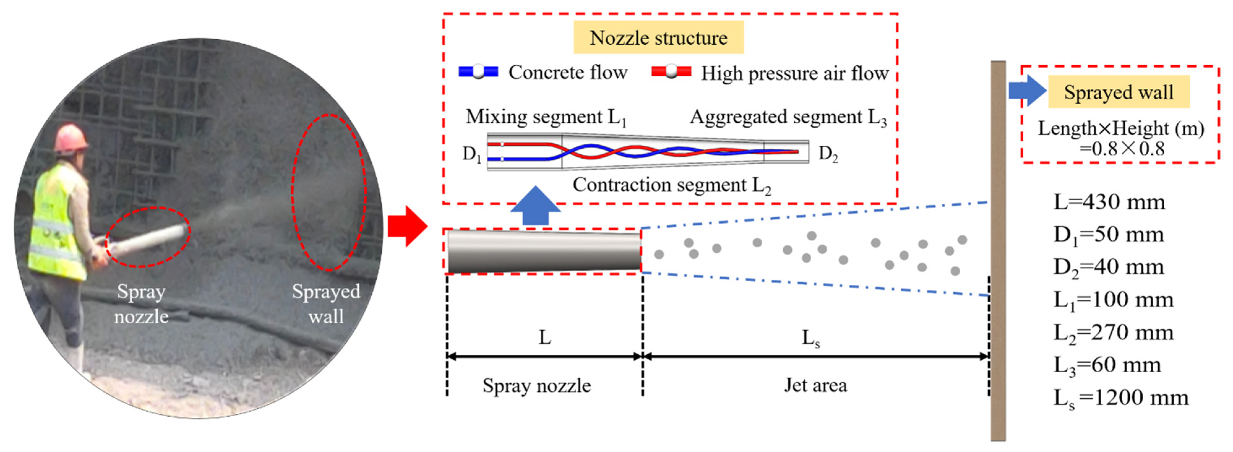
3.1. Operating Condition and Geometric Modeling

According to the actual construction characteristics of shotcrete, a geometric model consisting of a nozzle structure, jet area, and sprayed wall was constructed in this study. As shown in Figure 1, the nozzle structure can be divided into the front mixing section (L₁), the middle contraction section (L₂), and the rear aggregate section (L₃) to achieve the uniform mixing of concrete materials, secondary acceleration, and a stable jet flow, respectively. The distance between the nozzle and the sprayed wall was set to 1.2 m, following the current national standard ‘Technical code for the engineering of ground anchorages and shotcrete support’ (GB50086-2015) [36].

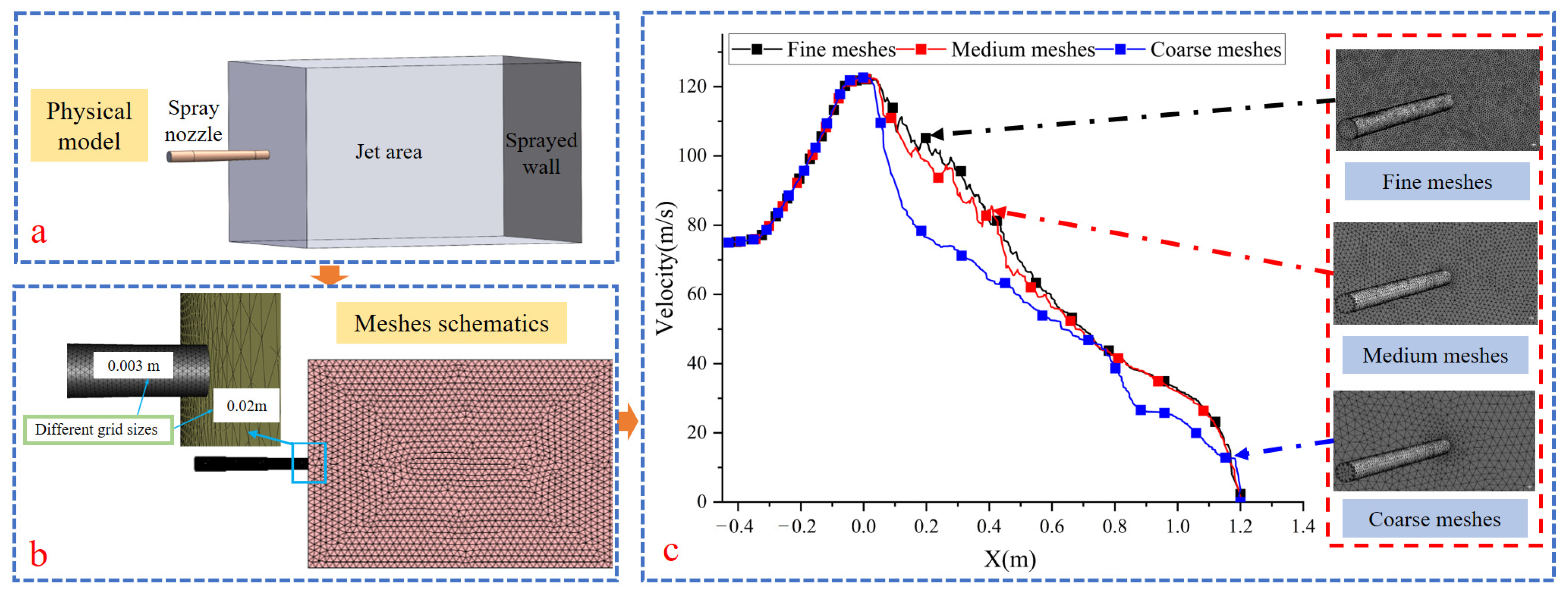
3.2. Meshing and Independence Verification

As shown in Figure 2a, a physical model of the wet-shotcrete particle jet flow field was established. In order to guarantee the speed and accuracy of the simulation calculation, the physical model was meshed using various-sized unstructured meshes for the nozzle and jet areas (Figure 2b). The mesh sizes of the nozzle structure and jet flow field area were 0.003 m and 0.02 m (medium meshes). The mesh quality tended towards 1, and there were no negative-volume meshes.

The mesh quantity dramatically affected the accuracy of the transient simulation results. A larger number of meshes could reduce discrete errors but increased rounding errors. Therefore, mesh independence verification was conducted to verify that the dispersion and rounding errors were acceptable, and that the meshes did not interfere with the simulation results [37,38]. Three kinds of different discrete meshes with different densities were generated, which were denoted as fine meshes, medium meshes, and coarse meshes. The average mesh quality was above 0.7 in all three cases.

The continuous-phase velocities on the X-axis in the three cases are shown in Figure 2c. It could be seen that the values in the three cases showed similar trends. The simulation results of the three meshes were basically the same inside the nozzle, with a difference of about 1% between the coarse meshes, medium meshes, and fine meshes. In the jet area, the results acquired for the coarse meshes differed significantly from those obtained for the fine meshes, with a maximum difference of about 25%. There were differences between the simulation results corresponding to the medium meshes and fine meshes, with a maximum error of about 4%, which did not compromise the accuracy of the simulation results. Therefore, it could be considered that the medium meshes had already met the requirement of meshing independence and guaranteed the simulation accuracy.

3.3. Simulation Parameters and Conditions

3.3.1. Rationality Assumption

In the wet-shotcrete-spraying process, the flow state of the concrete and air in the nozzle and the movement of the concrete and air in the jet area were extremely complex. To ensure the authenticity and accuracy of the simulation, several assumptions were made about the granular jet area: only the continuous phase (air) and discrete phase (concrete coarse aggregate particles with cement paste attached to the surface) were considered; only the movement of the working medium was studied, without taking into account the change in temperature or the hydration reaction of the cement; the deformation of the working medium due to the collision with the solid wall during the flow was ignored.

3.3.2. Continuous-Phase-Condition Parameters

The boundary conditions for the continuous-phase calculations were set by ANSYS Fluent. Pressure-based solvers and time-based transient calculations were used to calculate the gas–solid two-phase flow [39]. The continuous flow in the nozzle was completely turbulent, and the standard k-ε model was used to calculate the complex shear turbulence [40,41]. The Euler–Lagrange model was used to describe the gas–solid coupling in the flow fields. Furthermore, the Wen–Yu drag model was used to calculate the solid drag force [35]. According to the working air volume of the wet-spraying machine, an inlet wind velocity of 75 m/s was obtained. The air inlet was the velocity inlet, the outlet boundary of the jet flow field was the pressure outlet, and the pressure value was atmospheric pressure. The nozzle-internal-wall and sprayed-wall conditions were non-slip and stationary. The details of the parameters and operating conditions are listed in

Table 1. CFD simulation parameters.

Items	Details		Parameters
Computational model	Multiphase flow model		Euler–Lagrange
	Turbulence model		Standard k-ε
Boundary condition	Inlet-boundary type		Velocity inlet
	Outlet-boundary type		Pressure outlet
	Turbulence intensity	Inlet	3.37239%
		Outlet	4.2%
Materials	Air	Density [kg/m3]	1.225
		Viscosity [kg/(m·s)]	1.7894 × 10−5
Solution	Pressure velocity coupling		Phase-coupled SIMPLE
	Time type		Transient
	Initialization		Standard

.

3.3.3. Discrete-Phase-Condition Parameter

The coarse-aggregate particle size had a more significant effect on the rebound rate of the spraying than the shape, and the velocity of the aggregates was mainly related to the particle size and not to the shape [42]. In conclusion, coarse aggregates were replaced by spherical particles with different sizes in the simulation to easily observe the trajectories of the particles and the rebound phenomenon of the particle collision with the wall. According to Fuller grading, the masses of the coarse aggregates of different sizes in the wet shotcrete were obtained, which basically conformed to the Gaussian distribution law. The particle model and mass distribution are shown in Figure 3.

The mass flow rate of the concrete within 1 s of the spraying time could be roughly calculated based on the concrete flow rate. The final mass of the concrete flowing through the nozzle inlet section per unit time was 4.75 kg. The total masses of the five particle sizes, 4, 6, 8, 10, and 12 mm, were 11.4%, 24.3%, 32.6%, 21.5%, and 10.2%, respectively.

$$m_f={\rho S_{t}v}_b$$

(16)

where $m_f$ is the mass of the concrete entering the nozzle inlet per unit time; $\rho$ is the density of the concrete; $S_t$ is the cross-sectional area of the transport pipe; $v_b$ is the pumping velocity of the concrete.

The concrete particle–particle and particle–wall contact parameters have been given in previous studies [43]. However, there were some minor differences in the concrete proportioning in this study compared with those of the previous studies. To avoid the effect of the particle properties of the wet shotcrete on the simulation, the correction of previous calibration results was improved by a basic contact parameter experiment. Finally, the contact property parameters were obtained. To simulate the surface of aggregates covered with a layer of cement mortar, the contact radius of the particles was greater than the physical radius by 1.5 mm. The final DEM simulation parameters are shown in

Table 2. DEM simulation parameters.

Item	Details	Index	Value
Materials	Steel	Density [kg/m3]	7800
		Poisson ratio [-]	0.35
		Shear modulus [Pa]	8.00 × 108
	Particles	Density [kg/m3]	2100
		Poisson ratio [-]	0.3
		Shear modulus [Pa]	2.00 × 107
Interaction	Particle–Particle	Coefficient of restitution	0.35
		Coefficient of static friction	1.15
		Coefficient of rolling friction	0.15
		Contact model [-]	Hertz–Mindlin with bonding
		Normal stiffness per unit area [N/m3]	1.00 × 109
		Tangential stiffness per unit area [N/m3]	5.00 × 108
		Critical normal stress/shear stress [Pa]	500,000
	Particle–Steel	Coefficient of restitution	0.35
		Coefficient of static friction	1
		Coefficient of rolling friction	0.15
Particle generation	Factory type [-]		Dynamic
	Generation rate [kg/s]		4.75
Time step	1.00 × 105

. Altair’s EDEM software was used for the DEM simulation.

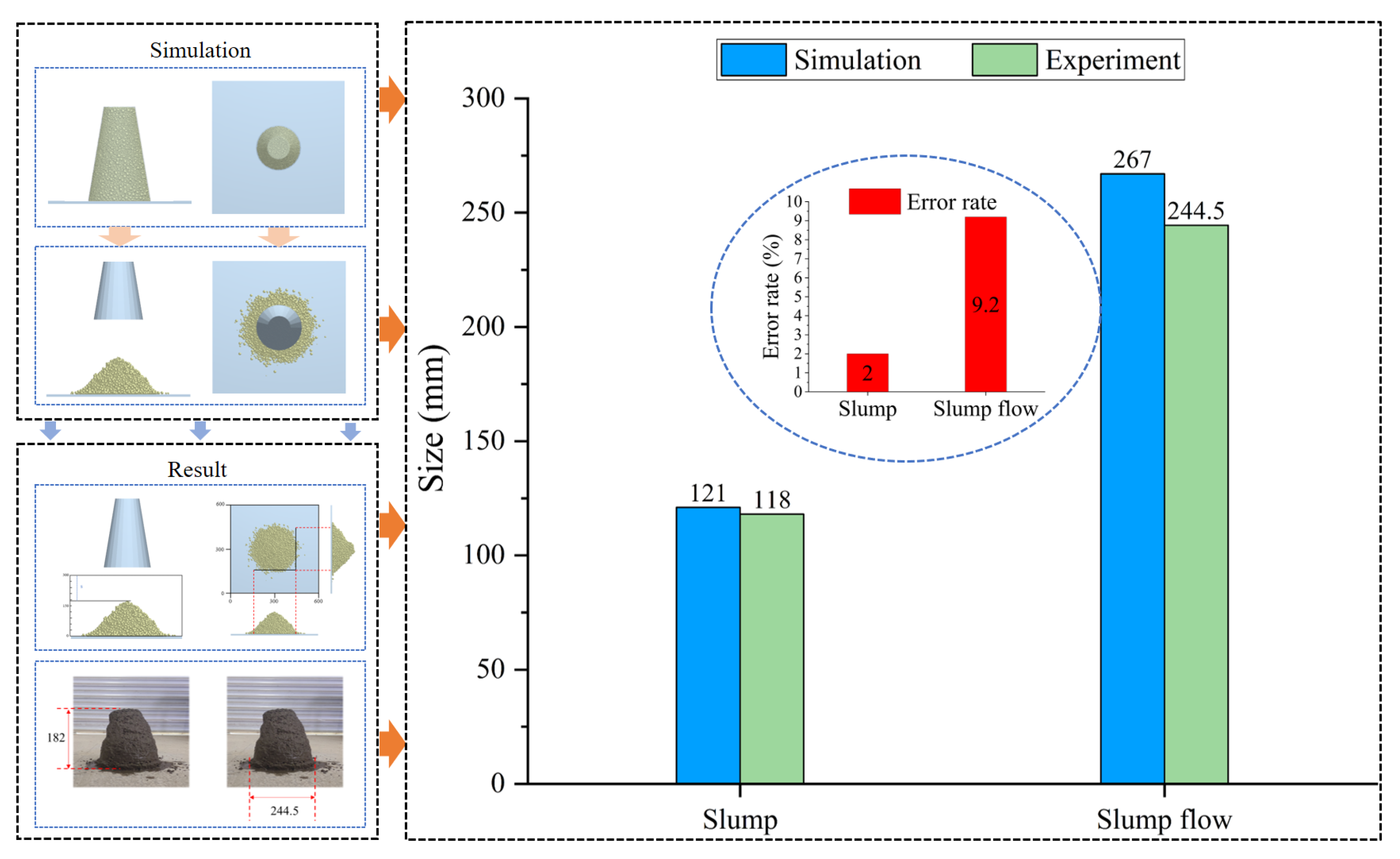
3.4. Experimental Verification

Continuous- and discrete-phase data, which were difficult to obtain through on-site experiments, were obtained through CFD-DEM-coupled simulation. In this paper, collapse simulations were performed to verify the reliability of the simulation parameters to ensure the consistency between the numerical and experimental results.

According to the ‘Technical code for the engineering of ground anchorages and shotcrete support’ (GB50086-2015), the experimental concrete collapse ratio was determined to ensure the fluidity and cohesiveness of the shotcrete, and the ratio of cement, stone, sand, and water was determined as 1:1.5:2.625:0.6. A slump cone with a top diameter of 100 mm, a bottom diameter of 200 mm, and a height of 300 mm was used for the slump, and the concrete was divided into three stages and filled into the slump cone. After each stage of filling, it was compacted and smoothed with a tamping hammer, and the cone was pulled up when it was filled. The height of the highest point of the concrete and the diameter of the bottom were measured after collapsing, and the slump and expansion were obtained. A slump-cone model with a top diameter of 100 mm, a bottom diameter of 200 mm, and a height of 300 mm was used for the slump simulation experiment. The slump-cone model was filled multiple times with the particle-filling method until it was fully filled, and then the model was lifted upwards and the height and bottom diameter of the concrete particles were measured. The numerical simulation results were compared with the experimental results, and the error was obtained.

The simulation process and experimental results are shown in Figure 4. The comparison between the collapse simulation results and on-site results showed that the collapse level was 121 mm with an error of 2%, and the extension was 267 mm with an error of 2%. Because the Hertz–Mindlin model with bonding could only be applied to interparticle bonding, there was no bonding between the particles and the collapsed cylinder wall. So, the expansion error in the simulation results was significantly greater than the collapse error, and an error of 9.2% was within the acceptable limits. The 2% error between the collapse simulation and the field test indicated that the interparticle-bonding parameters and the numerical simulation results were highly reliable.

4. Results and Analysis

4.1. Continuous-Phase Simulation Results

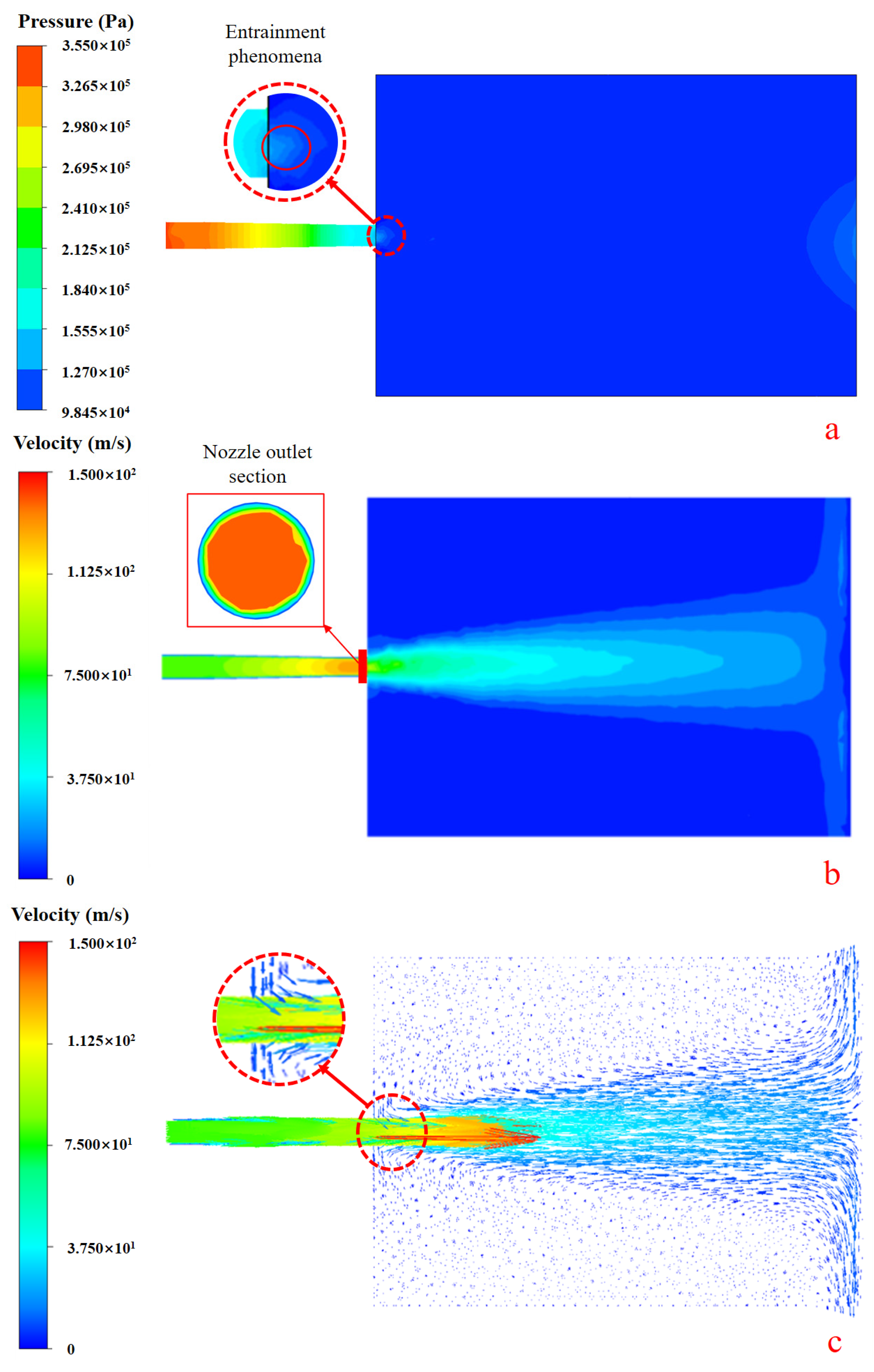
4.1.1. Pressure-Drop Analysis

Figure 5 shows the gas contours of the pressures and velocities, and the gas velocity vector on the Z = 0 section. As can be seen from Figure 5a, the static pressure drop in the jet flow field decreased from the nozzle inlet to the nozzle outlet with excellent symmetry. The static pressure drop of the gas at the nozzle outlet was reduced to 20,000 Pa, and the pressure drop in the jet area was atmospheric pressure. In addition, it was evident that there was a low-pressure zone at the nozzle outlet. As the continuous-phase flow rate increased, the pressure at this point decreased, and the air was sucked into it, forming a high-pressure jet entrainment. The direction of the velocity vector at the nozzle outlet in Figure 5c shows that the air near the nozzle outlet was being sucked into the low-pressure zone at the nozzle outlet.

4.1.2. Velocity Analysis

Figure 5b shows the continuous-phase velocity distribution at the Z = 0 cross section and the nozzle exit cross section. The continuous phase in the nozzle gradually increased in velocity along the center axis of the nozzle, and the velocity was roughly distributed symmetrically along the axis. The continuous-phase velocity reached the maximum at the nozzle outlet, the velocity parameters of the continuous-phase cross section at the nozzle outlet were circularly symmetric, and the outlet center velocity reached the maximum of 150 m/s. The continuous-phase velocity at the nozzle wall was the lowest, but the velocity was still higher than 32 m/s, decreasing the collision behavior between the particles and nozzle inner wall to guarantee an appropriate spraying distance.

Figure 5b,c show that the velocity of the high-pressure air decreased sharply after entering the jet area due to the large velocity difference between the high-pressure air and the air near the nozzle. Friction turbulence occurred after contacting the air around the nozzle outlet, resulting in a sudden decrease in the continuous-phase velocity to 80 m/s. A diffusion phenomenon occurred after the continuous phase was ejected from the nozzle. The continuous phase diffused from the jet axis to the periphery, and the continuous-phase velocity on the jet axis gradually decreased. When the continuous phase reached the sprayed wall, the velocity gradually decreased along the central axis towards the surrounding area. Subsequently, the wind direction became parallel to the wall, and the velocity dropped to around 6 m/s due to the obstruction of the wall.

4.2. Discrete-Phase Simulation Results

4.2.1. Particle Trajectories

Figure 6 shows the trajectories of the particles in the jet flow field at different moments before the steady state of the particle flow. The streamline represents the displacement of the particle at two time points before and after 0.01 s of movement. The streamlines of the particle trajectories show that it took around 0.3 s for the particle flow to reach a steady state. The volume of the particles in the nozzle gradually increased and was evenly distributed during the period before the jet was stabilized (Figure 6a). The particle flow was injected into the jet area at a certain diffusion angle by the combined action of the continuous phase and the nozzle structure. Furthermore, the diffusivity of the particle flow became more pronounced with the increasing jet distance, but the majority of particles still tended to move along the central axis of the jet (Figure 6b–d). Figure 6e,f show that the rebound distance after the particles hit the wall increased gradually, and the rebound direction was dispersed.

Figure 7 shows the streamlines of the particle trajectories at 0.5 s and 0.9 s in the steady state of the particle flow jet. In the stable jet stage, the particle distribution was more dispersed and homogeneous, and the trajectory tended to be uniform. The main area of the particle impact with the sprayed wall was defined as the effective jet area for the shotcrete. As shown in Figure 7, the effective jet area of the particle flow moved below the central axis of the jet under the action of gravity, it took from 0.15 to 0.2 s for the five types of particles to reach the wall from the nozzle outlet, and the particles can be considered free-falling bodies in the vertical plane. According to the displacement formula of free-falling bodies (Formula (17)), the particle flow produced a deviation of approximately 0.15 m in the Y direction. When the jet reached 0.9 s, the particle flow jet remained stable and uniform, rebound particles increased, and some rebound particles crossed the nozzle outlet section.

$$h=\frac{1}{2}g{t}^2$$

(17)

The velocity vector of the particles in the jet area at t = 0.5 s was selected to analyze the particle diffusion angle. Figure 8 shows the particle velocity vector in the t = 0.5 s jet area. Small particles were defined as 4 mm and 6 mm particles, and large particles were defined as 10 mm and 12 mm particles. The direction of the small-particle velocity vector had a more pronounced diffusion tendency than the direction of the large-particle velocity vector: the diffusion angle (α) was about 7° for large particles, and the β was about 12° for small particles. This phenomenon occurred because of the smaller mass of the small particles, which were more susceptible to continuous-phase action than the larger particles.

4.2.2. Particle Velocity

The velocities of the particles were the most important parameter in the analysis of the particle flow properties and were an intuitionistic result of the interaction between the continuous phase and the particles. The variation law of particle velocity was analyzed from the jet area and particle size.

Figure 9 shows the variation in the average velocities of particles of different sizes over time. It was found that there was no significant difference between the particles inside the nozzle at 0 s–0.025 s. The velocity increased steadily after the particles entered the jet area. At 0.15 s, the particles reached the wall, the particle velocity sharply decreased after collision with the sprayed wall, and the average velocities of the particles began to decrease. Smaller particles had higher velocities and reached the sprayed wall surface faster. Therefore, it could be summarized that the average velocities of the different-sized particles began to decrease at different times. By combining them in Figure 6, the time when the particles first reached the sprayed wall surface can be seen more clearly.

In the simulation of the particle flow jet, the particles had five different diameters. The velocities of the particles in the different jet areas were analyzed at t = 0.2 s. Figure 10 shows the particle velocities at different distances and the average velocities of the particles of different sizes in the jet area. It can be seen that the particles of different sizes inside the nozzle steadily accelerated their movements. Due to the low speed and the nozzle structure limitation of the particles, the velocity difference was not significant. After the particles entered the jet area, the difference in the velocities between the particles of different sizes became progressively larger, and the velocities of the small particles were generally greater than those of the large particles in the same area.

Figure 10 shows that the velocity increment of the particles of different sizes was the highest from (a) to (b), and that there was still a significant velocity increment from (b) to (c), while the velocity changes in the particles of different sizes from (c) to (d) generated some differences. The velocities of the small particles increased from (a) to (b) and from (b) to (c), while they decreased from (c) to (d). This phenomenon verified that the small particles more easily accomplished the acceleration, and the maximum velocity reached 25 m/s. However, when the velocity of the continuous phase decreased to a state in which the velocity could not support particle acceleration, the velocities of the small-size particles decreased, but they still remained 20 m/s in (d).

The velocities of the large particles increased in the different jet areas. They were generally around 14 m/s in (b), increased to around 18 m/s in (c), and reached around 19 m/s in (d). The results indicated that the large-size particles were also affected by the continuous phase, but it took longer for them to reach the peak velocity. The velocity difference may be because the particles of different sizes had different force areas and weights. Figure 5 and Figure 10 show that the peak particle velocity was in (b) and (c) of the jet area, small particles reached their maximum velocity in (b), large particles reached their maximum velocity in (c), and larger particles required a longer acceleration time to reach their maximum velocity.

The final particles reached and collided with the sprayed wall surface, resulting in particle energy loss. The velocity significantly decreased after the collision and rebound. Figure 11 shows the particle velocity vector near the sprayed wall at t = 0.5 s. The center dashed line represents the central axis of the jet. Area (a) represents the area 0.1 m away from the sprayed wall, and area (b) represents the area 0.2 m away from the nozzle outlet. Figure 11 shows that the rebound particle velocity in (a) was around 10 m/s, with a maximum velocity of around 8 m/s, and that the rebound velocity was within the normal range. The continuous phase played a negative role in the motion of the particles after the rebound of the particles, leading to the decrease in the velocities of the particles. Compared with (a), (b) was far from the sprayed wall, and the velocity of the rebound particles was significantly reduced with about 1.22 m/s–3.6 m/s. As shown in Figure 8, some particles had rebound distances exceeding the nozzle inlet section, and the particles were dispersed more widely, which might cause injury to construction personnel. However, the velocities of the rebound particles passing through the nozzle inlet section were relatively low, and the risk of harm to construction personnel could be within an acceptable range.

4.2.3. Particle Collision

The collision of concrete particles can change the particle motion state. The collision behaviors of the particles in the jet flow field mainly included three types: collision between the particles and the inner wall of the nozzle; interparticle collision; collision between the particles and the sprayed wall.

Taking the particle jet at 0.5 s as an example, the force of the particle collision was analyzed. At this time, the particle flow was in a stable jet state. The distribution of the collision forces between the particles and the inner wall of the nozzle is shown in Figure 12a. The contact between the particles and the inner wall of the nozzle was mostly concentrated in the mixing section at the front of the nozzle, and the direction of the collision force was irregular, with a maximum value of around 6.2 × 10⁻³ N. As the particle movement distance increased, the particles tended to move towards the center axis of the jet, and the number of particle collisions in the aggregate section at the rear of the nozzle decreased significantly.

When the particles entered the jet area, the velocity difference between the particles of different sizes increased, and the rebound direction of the particles dispersed after hitting the wall, resulting in two different interparticle collision behaviors. The first type involved the slower increase in the velocities of the large-size particles compared with those of the small-size particles after leaving the nozzle. As shown in Figure 12b,c, due to the larger velocities of the small-size particles, the large-size particles were impacted with collision forces between 2.92 × 10⁻³ and 5.7 × 10⁻³ N by the small-size particles. This collision behavior often occurred near the nozzle outlet. As the spray distance increased, the probability of its occurrence greatly decreased. The second type involved the collision of some of the rebound particles with the jet particles during the rebound process of the particles hitting the wall. The location of this collision behavior was uncertain due to the irregular rebound direction, as shown in Figure 12d, exhibiting a collision force of about 5.7 ×10⁻³ N.

As soon as the particles came into contact with the wall, collision behavior between them occurred and displayed consecutiveness. As the jet progressed, the number of collisions between the particles and the wall increased. The duration of the collision between the particles and the wall was approximately 1 × 10⁻³ s, making it difficult to capture the collision behavior. However, it was possible to determine whether a collision had occurred based on the presence or absence of collision force between the particles and the wall. Figure 12e shows the collisions of four particles with the wall. The magnitudes and directions of the collision forces varied due to differences in the collision velocities and directions.

The collision forces generated by the particle collisions ranged from 2.0 × 10⁻³ N to 6.2 × 10⁻³ N. Only taking the impact of the collision forces on the particle acceleration into consideration, the magnitude of the acceleration caused by the collision forces on the particles could be obtained according to Newton’s second law: $F=ma$. Figure 13 shows the range of accelerations of the different particles under three types of collisions. The graph shows the range of accelerations generated by different particles due to collision. The smaller the particle size, the greater the impact of the collision force. The acceleration of the 4 mm particles reached 37.58 m/s², while the maximum acceleration of the 12 mm particles was only 1.25 m/s². These results confirmed that the motion state of the small particles was more likely to be affected by the continuous phase, which was consistent with the previous analysis.

The collision behavior between the particles and the inner wall of the nozzle gradually decreased with the movement of the particles, and the collisions between the particles were uncertain. The collision between the particles and the sprayed wall was stable and continuous, with the highest frequency. Figure 14 shows the number of collisions within a range of 0.1 m from the sprayed wall (between particles, between particles and the sprayed wall, and between 0 and 0.9 s). The number of collisions between the particles and the sprayed wall was 19.51 times that of the collisions between particles. This indicated that the collision between the particles and the sprayed wall was the main collision mode of the wet-shotcrete rebound. The motion state and properties of the particles (such as the velocity and particle size) when colliding with the sprayed wall were the main factors affecting the collision force. Therefore, regulating the velocity and particle size distribution of particles can reduce the rebound of concrete materials.

5. Conclusions

In this paper, coupled CFD-DEM was used to simulate the motion of coarse aggregate particles of different sizes in the granular flow jet of wet shotcrete. The pressure drop and velocity variation in high-pressure air (continuous phase), the trajectories and distributions of the particles (discrete phase), the distribution of the particle velocity field, and the collision rebound behaviors of the particle collisions were obtained, revealing the factors affecting the stability of the wet-shotcrete jet.

(1)

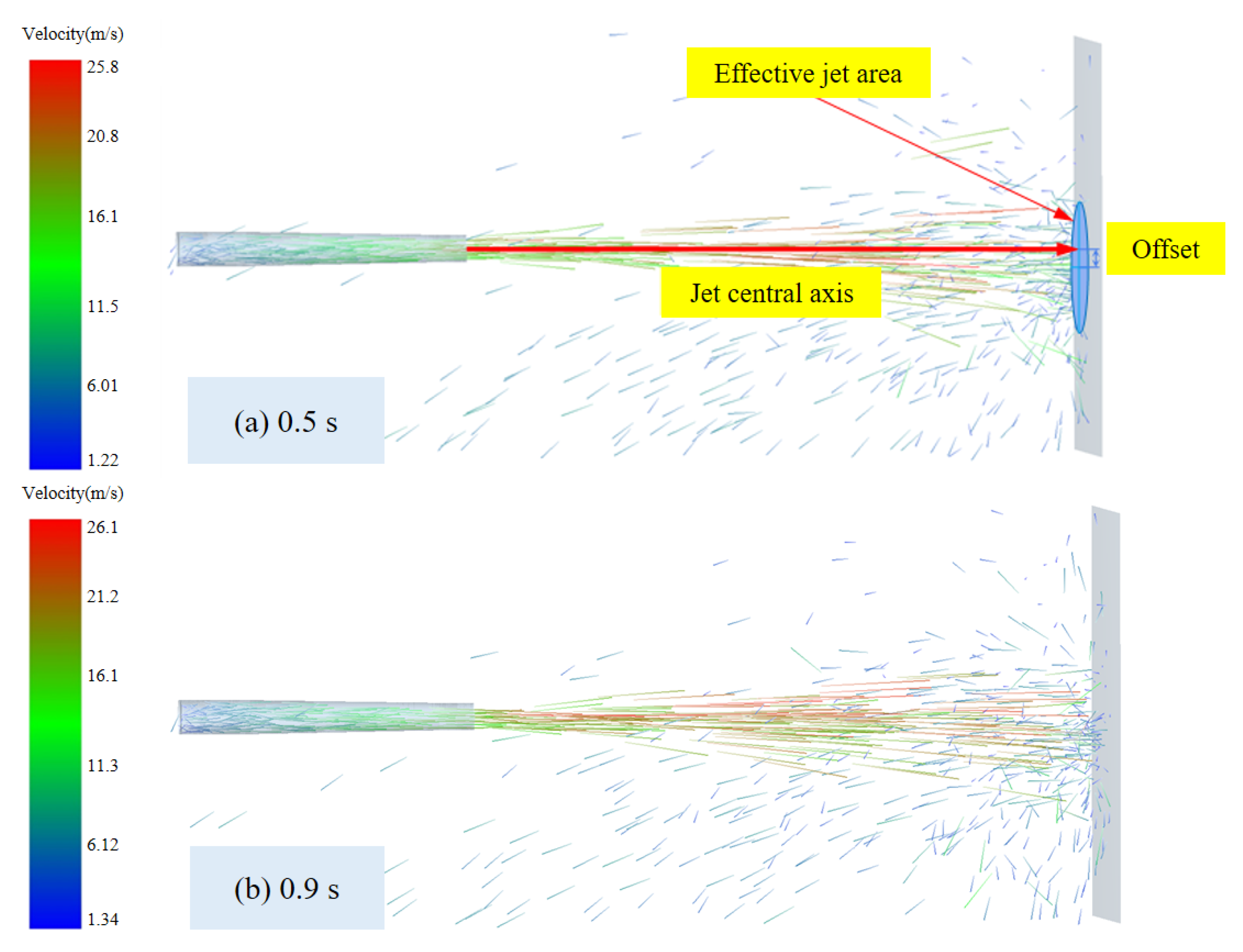
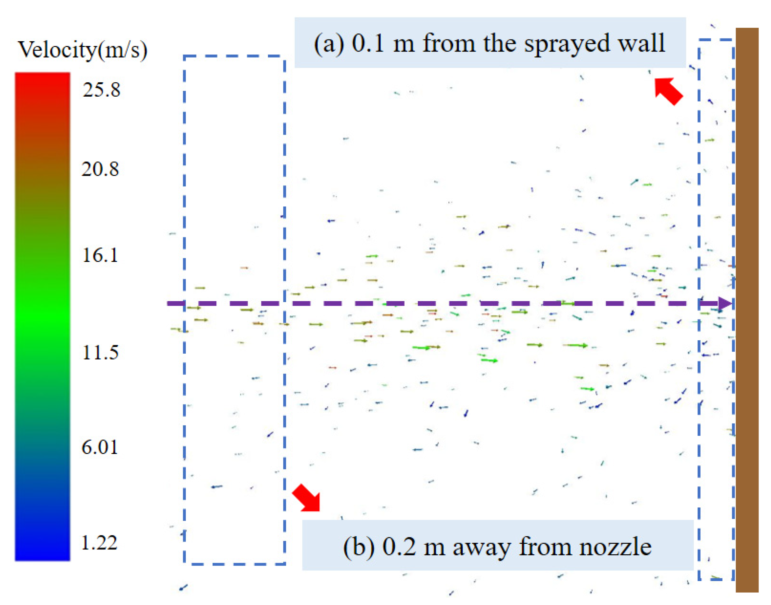
The velocity and pressure drop of the continuous-phase jet of wet shotcrete were symmetrical and continuous, which were the prerequisites for a stable jet of shotcrete. The continuous phase at the nozzle exit reached its maximum velocity, resulting in a suction effect that led to entrainment and caused the surrounding air to flow to the exit. After the continuous phase entered the jet area, the velocity gradually reduced with the increase in the jet distance, and when it reached the sprayed wall, the continuous-phase velocity direction became parallel to the wall, and the velocity decreased to about 6 m/s. This indicated that, after the particles left the nozzle, the continuous phase could still provide kinetic energy for them;

(2)

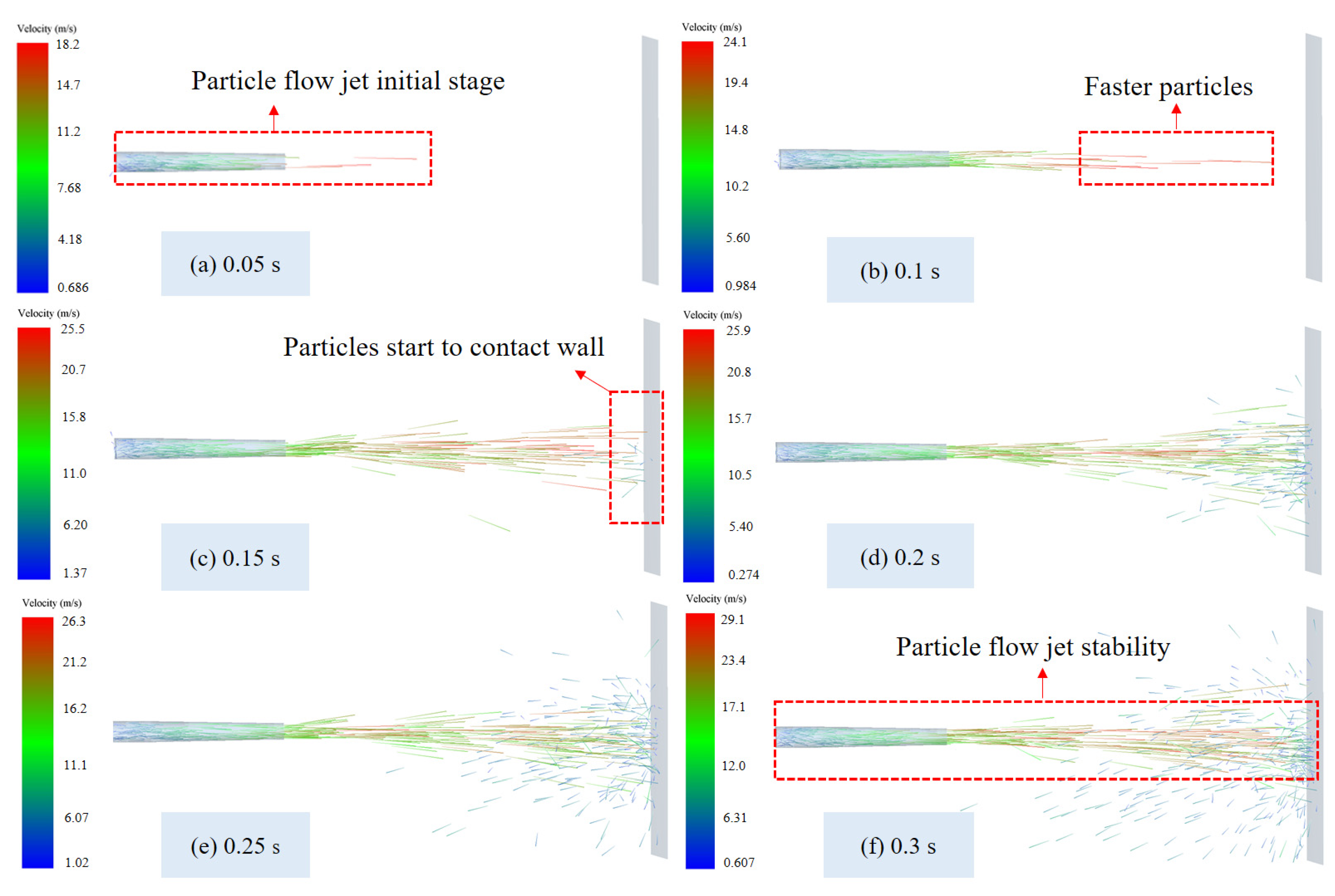
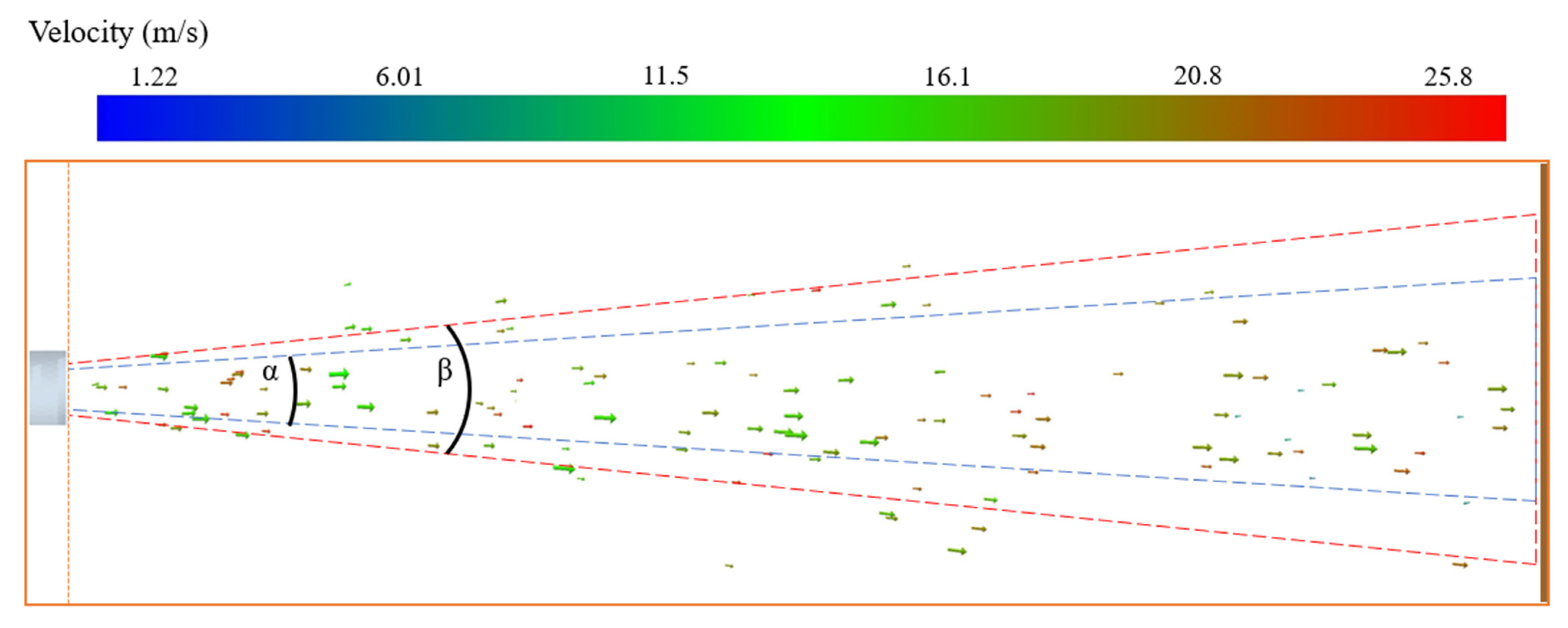
The particle flow reached a steady jet state at around 0.3 s. The effective jet area of the particle flow was deflected downwards by gravity, and the degree of deviation depended on the spraying distance and particle velocity. In the Y plane, the diffusion angles of the large particles and small particles were approximately 7° and 12°, respectively. The large particle jet was more concentrated, which indicated that large particles were more likely to be sprayed into the designated spraying area;

(3)

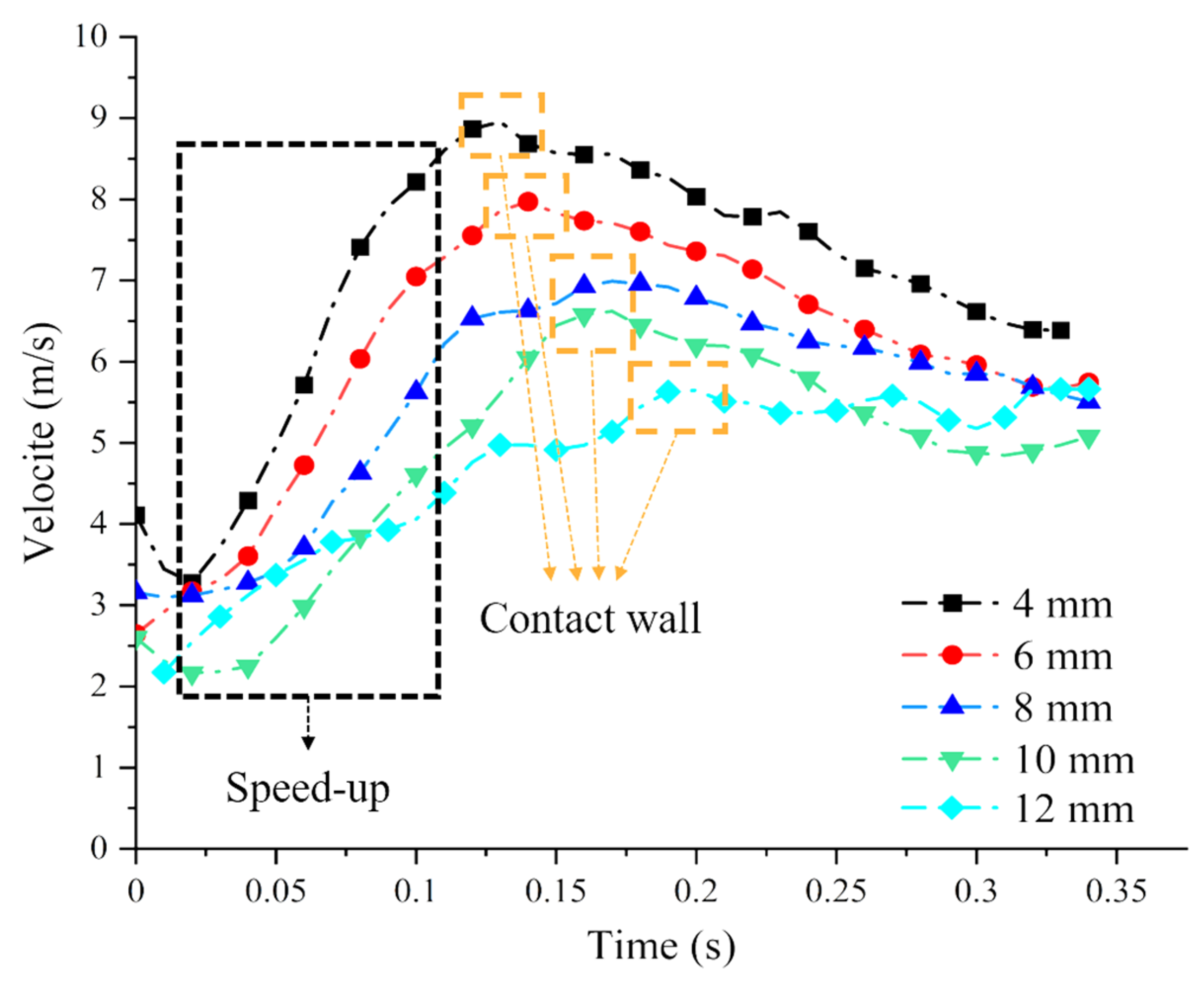
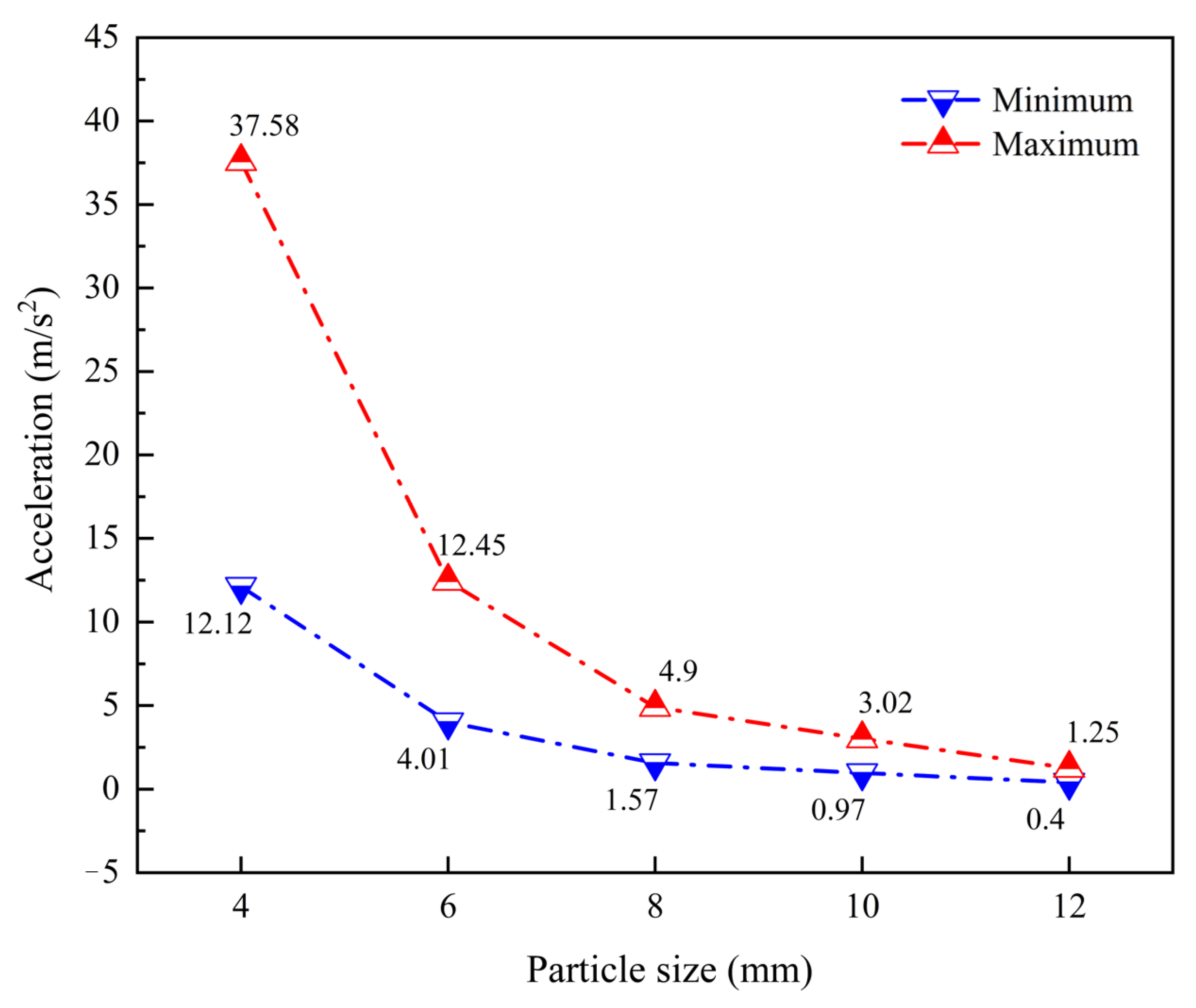
The velocity difference between the particles of different sizes in the nozzle was small and became significant as the particles entered the jet area. In the different jet areas, the average velocity of the small particles was greater than that of the large particles, and the maximum velocity of the 4 mm particles was 25 m/s, while that of the 12 mm particles was 19 m/s. The large particles required a longer acceleration time to reach their maximum velocity than the small particles;

(4)

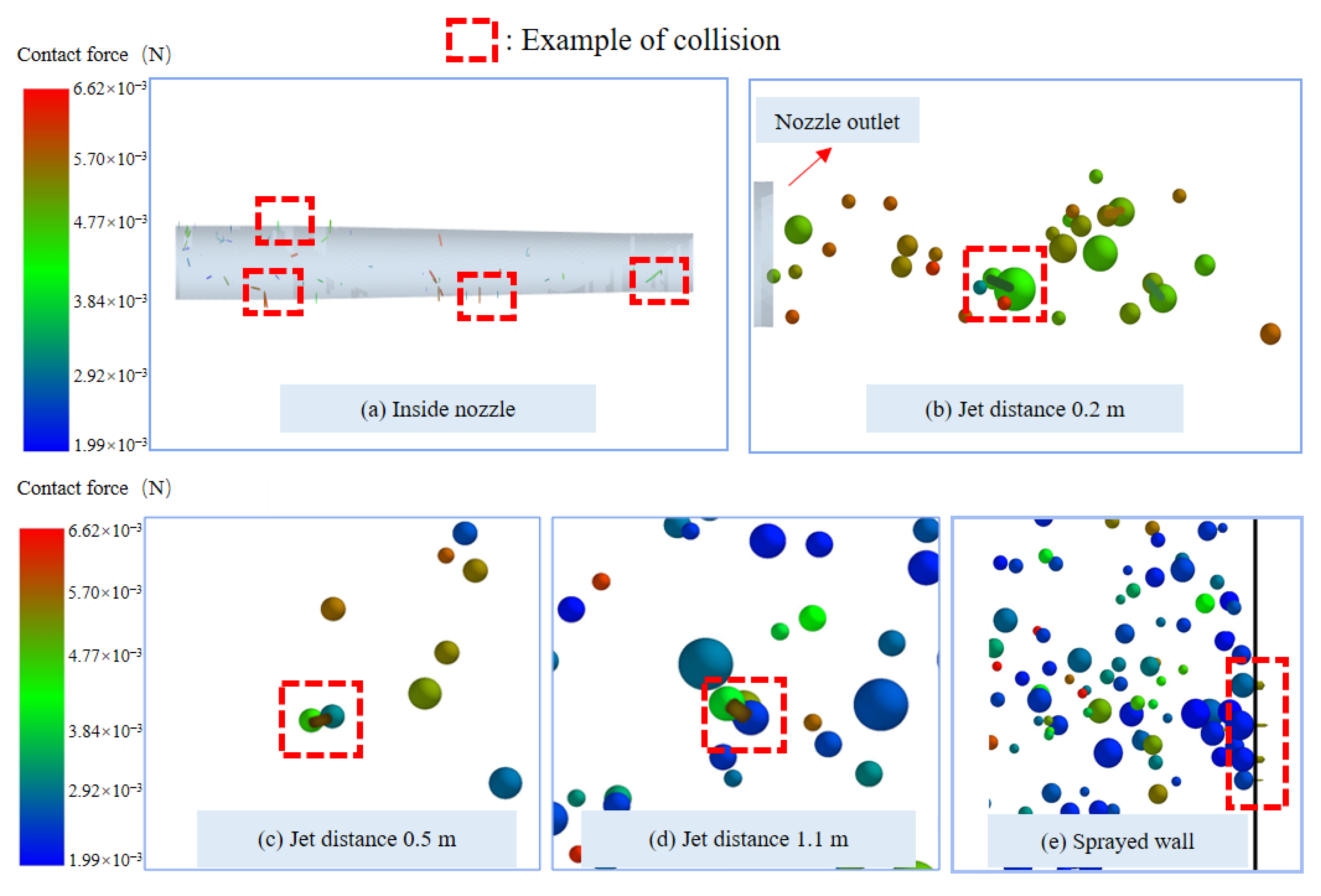
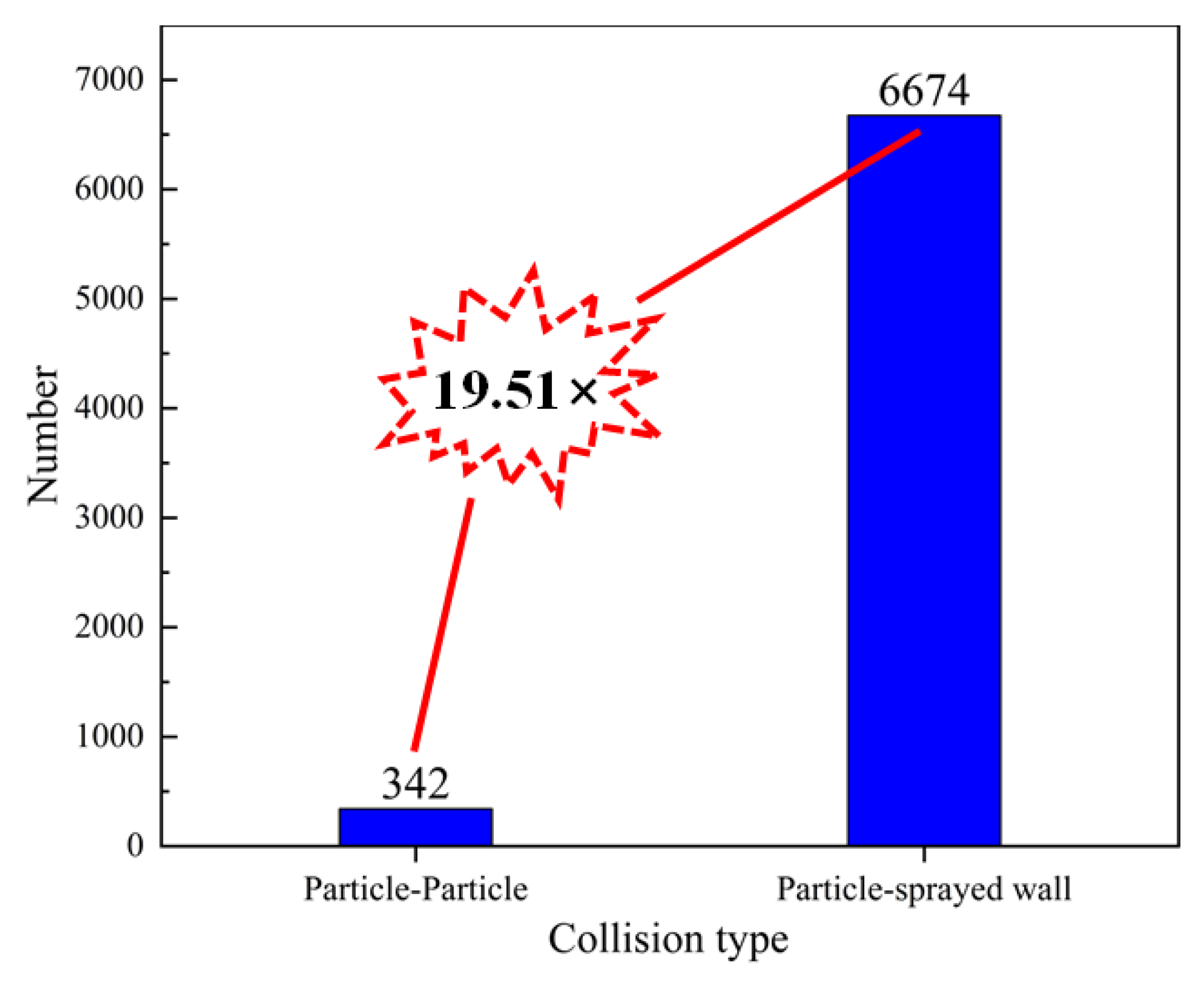
The collision took three forms: particle collision with the inner wall of the nozzle, interparticle collision, and particle collision with the sprayed wall. The collision between the particles and the sprayed wall was the main cause of the rebound, and the collision rebound angle near the sprayed wall was uncertain. Due to differences in the particle size and mass, the small particles were more susceptible to impact and more likely to rebound from collisions compared to the large particles.

In conclusion, in order to reduce rebound, the particle velocity could be controlled by adjusting the air volume and air pressure of the injection, and the velocity when the particles reach the sprayed wall could be adjusted by adjusting the injection distance. It is hoped that future studies can be conducted on the use of the air volume to adjust the particle velocity, and that the relationship between the particle velocity and rebound rate when the particles hit the wall can be obtained so that the rebound problem of shotcrete can be controlled better.

References

1. Garshol, K. Shotcrete: International practices and trends. In Proceedings of the Specialist Techniques and Materials for Concrete Construction: Proceedings of the International Conference, Scotland, UK, 8–10 September 1999; p. 163. [Google Scholar]
2. Knight Brad, W.; Rispin, M.; Clegg, I. Wet-Mix Shotcrete as a Material, Process, and Ground Control Component of a 21st Century Underground Mining Operation; Shotcrete for Underground Support X: Reston, VA, USA, 2012; pp. 298–306. [Google Scholar]
3. Watanabe, T.; Hosomi, M.; Yuno, K.; Hashimoto, C. Quality evaluation of shotcrete by acoustic emission. Constr. Build. Mater. 2010, 24, 2358–2362. [Google Scholar] [CrossRef]
4. Ding, J.; Wu, Y.; Lei, Y. Several on-site process experiments using nanomaterials to improve the rebound rate and strength of ordinary wet dry sprayed concrete. In Proceedings of the 2018 Academic Exchange Conference of the Sichuan Hydroelectric Engineering Society and the Construction Technology Exchange Conference of the Six Provinces (Regions) of Sichuan, Yunnan, Guangxi, Hunan, Guangdong, and Qinghai, Chengdu, China, 15 November 2018. [Google Scholar]
5. Wang, Z.; Chen, Y.; Sun, J.; Xia, H. Analysis of erosion wear of filling slurry on reducing pipes. J. Shandong Univ. Sci. Technol. (Nat. Sci.) 2022, 4, 39–46. [Google Scholar]
6. Cheng, W.M.; Liu, W.; Nie, W.; Zhou, G.; Cui, X.F.; Sun, X. The Prevention and Control Technology of Dusts in Heading and Winning Faces and Its Development Tendency. J. Shandong Univ. Sci. Technol. (Nat. Sci.) 2010, 29, 77–81. [Google Scholar]
7. Armelin, H.S.; Banthia, N. Mechanics of aggregate rebound in shotcrete—(Part I). Mater. Struct. 1998, 31, 91–98. [Google Scholar] [CrossRef]
8. Armelin, H.S.; Banthia, N. Development of a general model of aggregate rebound for dry-mix shotcrete—(Part II). Mater. Struct. 1998, 31, 195–202. [Google Scholar] [CrossRef]
9. Jolin, M.; Lemay, J.D.; Ginouse, N.; Bissonnette, B.; Blouin-Dallaire, É. The effect of spraying on fiber content and shotcrete properties. In Proceedings of the Shotcrete for Underground Support XII, Singapore, 15 October 2015. [Google Scholar]
10. He, W. Research on Performance and Composition Design Methods of High Air Content Wet Sprayed Concrete. Ph.D. Thesis, Chang’an University, Xi’an, China, 2014. [Google Scholar]
11. Marc, J.; Denis, B. Effects of Particle-Size Distribution in Dry Process Shotcrete. ACI Mater. J. 2004, 101, 131–135. [Google Scholar]
12. Zhang, Y.; Zhang, J. Analysis of the influence of springback rate of wet-sprayed concrete based on aggregate characteristic analysis. In Structural Seismic and Civil Engineering Research; CRC Press: Boca Raton, FL, USA, 2023; pp. 150–155. [Google Scholar]
13. Cui, Y.; Tan, Z.; Zhou, Z.; Wu, J.; Wang, J. Preparation and application of low rebound liquid alkali-free accelerator for shotcrete. Constr. Build. Mater. 2023, 367, 130220. [Google Scholar] [CrossRef]
14. Liu, Z.; Bian, W.; Pan, G.; Li, P.; Li, W. Influences on Shotcrete Rebound from Walls with Random Roughness. Adv. Mater. Sci. Eng. 2018, 2018, 7401358. [Google Scholar] [CrossRef]
15. Chen, L.; Sun, Z.; Liu, G.; Ma, G.; Liu, X. Spraying characteristics of mining wet shotcrete. Constr. Build. Mater. 2022, 316, 125888. [Google Scholar] [CrossRef]
16. Pan, G.; Li, P.; Chen, L.; Liu, G. A study of the effect of rheological properties of fresh concrete on shotcrete-rebound based on different additive components. Constr. Build. Mater. 2019, 224, 1069–1080. [Google Scholar] [CrossRef]
17. Krenzer, K.; Mechtcherine, V.; Palzer, U. Simulating mixing processes of fresh concrete using the discrete element method (DEM) under consideration of water addition and changes in moisture distribution. Cem. Concr. Res. 2019, 115, 274–282. [Google Scholar] [CrossRef]
18. Li, Z.; Cao, G.; Guo, K. Numerical method for thixotropic behavior of fresh concrete. Constr. Build. Mater. 2018, 187, 931–941. [Google Scholar] [CrossRef]
19. Wu, J.; El Naggar, M.H.; Li, X.; Wen, H. DEM analysis of geobag wall system filled with recycled concrete aggregate. Constr. Build. Mater. 2020, 238, 117684. [Google Scholar] [CrossRef]
20. Hærvig, J.; Kleinhans, U.; Wieland, C.; Spliethoff, H.; Jensen, A.L.; Sørensen, K.; Condra, T.J. On the adhesive JKR contact and rolling models for reduced particle stiffness discrete element simulations. Powder Technol. 2017, 319, 472–482. [Google Scholar] [CrossRef]
21. Cui, W.; Yan, W.-S.; Song, H.-F.; Wu, X.-L. Blocking analysis of fresh self-compacting concrete based on the DEM. Constr. Build. Mater. 2018, 168, 412–421. [Google Scholar] [CrossRef]
22. Su, C.; Wu, Z.; Zheng, X. Analysis of Rebound Rate of Wet Shotcrete Based on Experiment and Discrete Element Method. Shock Vib. 2022, 2022, 1840580. [Google Scholar] [CrossRef]
23. Tavangar, T.; Hosseinpoor, M.; Marshall, J.S.; Yahia, A.; Khayat, K.H. Discrete-element modeling of shear-induced particle migration during concrete pipe flow: Effect of size distribution and concentration of aggregate on formation of lubrication layer. Cem. Concr. Res. 2023, 166, 107113. [Google Scholar] [CrossRef]
24. Zhou, F. Research on Key Technologies for Pneumatic Conveying of Large Coal Particles. Ph.D. Thesis, China University of Mining and Technology, Xuzhou, China, 2022. [Google Scholar]
25. Zhao, H.; Zhao, Y. CFD-DEM simulation of pneumatic conveying in a horizontal pipe. Powder Technol. 2020, 373, 58–72. [Google Scholar] [CrossRef]
26. Jiang, S.; Chen, X.; Cao, G.; Tan, Y.; Xiao, X.; Zhou, Y.; Liu, S.; Tong, Z.; Wu, Y. Optimization of fresh concrete pumping pressure loss with CFD-DEM approach. Constr. Build. Mater. 2021, 276, 122204. [Google Scholar] [CrossRef]
27. Huang, W.; Yan, Z.; Sun, F.; Zhao, B.; Xue, S.; Zhou, B. Particle flow simulation study on the characteristics of Brazilian fracturing failure in layered shale. J. Shandong Univ. Sci. Technol. (Nat. Sci. Ed.) 2022, 41, 74–82. [Google Scholar]
28. Chen, J.; Li, H.; Zhu, Y.; Zhang, Y.; Tang, D.; Zhu, J.; Li, W.; Wang, K. Particle flow simulation study on the effect of stiffness differences on rock fracture. J. Shandong Univ. Sci. Technol. (Nat. Sci. Ed.) 2022, 41, 51–59. [Google Scholar]
29. El-Emam, M.A.; Zhou, L.; Shi, W.; Han, C.; Bai, L.; Agarwal, R. Theories and Applications of CFD–DEM Coupling Approach for Granular Flow: A Review. Arch. Comput. Methods Eng. 2021, 28, 4979–5020. [Google Scholar] [CrossRef]
30. Uzi, A.; Levy, A. Flow characteristics of coarse particles in horizontal hydraulic conveying. Powder Technol. 2018, 326, 302–321. [Google Scholar] [CrossRef]
31. Zhou, M.; Kuang, S.; Xiao, F.; Luo, K.; Yu, A. CFD-DEM analysis of hydraulic conveying bends: Interaction between pipe orientation and flow regime. Powder Technol. 2021, 392, 619–631. [Google Scholar] [CrossRef]
32. Yang, D.; Xing, B.; Li, J.; Wang, Y.; Hu, N.; Jiang, S. Experiment and simulation analysis of the suspension behavior of large (5–30 mm) nonspherical particles in vertical pneumatic conveying. Powder Technol. 2019, 354, 442–455. [Google Scholar] [CrossRef]
33. Crowe, C.T.; Schwarzkopf, J.D.; Sommerfeld, M.; Tsuji, Y. Multiphase Flows with Droplets and Particles; CRC Press: Boca Raton, FL, USA, 2011. [Google Scholar]
34. Potyondy, D.O.; Cundall, P. A bonded-particle model for rock. Int. J. Rock Mech. Min. Sci. 2004, 41, 1329–1364. [Google Scholar] [CrossRef]
35. Zhou, J.; Shangguan, L.; Gao, K.; Wang, Y.; Hao, Y. Numerical study of slug characteristics for coarse particle dense phase pneumatic conveying. Powder Technol. 2021, 392, 438–447. [Google Scholar] [CrossRef]
36. GB50086-2015; Technical Code for Engineering of Ground Anchorages and Shotcrete Support. Ministry of Housing and Urban-Rural Development of the People’s Republic of China: Beijing, China, 2015.
37. Yu, H.; Cheng, W.; Wu, L.; Wang, H.; Xie, Y. Mechanisms of dust diffuse pollution under forced-exhaust ventilation in fully-mechanized excavation faces by CFD-DEM. Powder Technol. 2017, 317, 31–47. [Google Scholar] [CrossRef]
38. Yu, H.; Cheng, W.; Wang, H.; Peng, H.; Xie, Y. Formation mechanisms of a dust-removal air curtain in a fully-mechanized excavation face and an analysis of its dust-removal performances based on CFD and DEM. Adv. Powder Technol. 2017, 28, 2830–2847. [Google Scholar] [CrossRef]
39. Olaleye, A.K.; Shardt, O.; Walker, G.M.; Van den Akker, H.E. Pneumatic conveying of cohesive dairy powder: Experiments and CFD-DEM simulations. Powder Technol. 2019, 357, 193–213. [Google Scholar] [CrossRef]
40. Chen, J.; Wang, Y.; Li, X.; He, R.; Han, S.; Chen, Y. Reprint of “Erosion prediction of liquid-particle two-phase flow in pipeline elbows via CFD–DEM coupling method”. Powder Technol. 2015, 282, 25–31. [Google Scholar] [CrossRef]
41. Zhou, C. Research on Wear Mechanism of Fluid Solid Two Phase Flow Transportation Pipeline Based on CFD-DEM Coupling. Master’s Thesis, Yunnan Agricultural University, Kunming, China, 2022. [Google Scholar]
42. Bindiganavile, V.; Banthia, N. Fiber reinforced dry-mix shotcrete with metakaolin. Cem. Concr. Compos. 2001, 23, 503–514. [Google Scholar] [CrossRef]
43. Ma, G. Development and Experimental Research of a New Type of Non Pulse Wet Spraying Machine. Ph.D. Thesis, Shandong University of Science and Technology, Qingdao, China, 2020. [Google Scholar]
Figure 1. Schematic diagram of the wet-shotcrete construction site and grain flow jet area.
Buildings 14 00977 g001
Figure 2. Meshing and mesh independence verification. (a) Physical model. (b) Meshing. (c) Mesh independence verification.
Buildings 14 00977 g002
Figure 3. Coarse-aggregate grading curve with particle model and mass share diagram.
Buildings 14 00977 g003
Figure 4. Collapse simulation and experimental verification process and results.
Buildings 14 00977 g004
Figure 5. Gas contours of pressures and velocities, and gas velocity vector on Z = 0 cross section. (a) Contours of pressures. (b) Contours of velocities. (c) Velocity vector of gas.
Buildings 14 00977 g005
Figure 6. Streamlines of particle trajectories at different moments before stabilizing the jet.
Buildings 14 00977 g006
Figure 7. Streamlines of particle trajectories at different moments after jet stabilization.
Buildings 14 00977 g007
Figure 8. Velocity vector and diffusion angle of particles in the jet area.
Buildings 14 00977 g008
Figure 9. Average velocities of particles of different sizes.
Buildings 14 00977 g009
Figure 10. Graph of particle velocities and average particle velocities in different jet areas.
Buildings 14 00977 g010
Figure 11. Vector plot of particle rebound velocities when colliding with a wall.
Buildings 14 00977 g011
Figure 12. Different collision behaviors of particles.
Buildings 14 00977 g012
Figure 13. Particle acceleration range caused by collision forces.
Buildings 14 00977 g013
Figure 14. The numbers of different collision types near the sprayed wall.
Buildings 14 00977 g014