1. Introduction
When it was first published in 1941, the National Building Code (NBC) of Canada included the latest information and knowledge on building science and engineering at that time. To sustain and update the NBC, the National Research Council (NRC) created the Division of Building Research and the Associate Committee on the National Building Code (ACNBC). The ACNBC prepared and published the “Code for Dwelling Construction” in 1950 and “A Building Code for Small Municipalities” in 1951. Later, two updated versions of the NBC were published in 1953 and then in 1960, after which newer editions of the code were printed more or less on a regular basis every five years [
1].
Limit state structural design philosophy was first introduced in the NBC in 1975. In such an approach, the load and resistance factors were based on the statistical variations of the applied forces on the structure and strength of the members. They were derived to give a uniform target reliability or consistent probability of failure, thus providing a consistent context for structural design and risk management. For steel structures, the NBC and CSA S16.1 combine to give a reliability index equal to 3.0 for structural members. A greater reliability index was used for bolted and welded connections so that the probability of the connector failing before the member was reduced and the more ductile mode of failure of the member was favored. Experience has shown that design and detailing following this approach result in economic structures, since the members are proportioned for a prescribed safety level through realistic load combinations and accurate modelling based on ultimate strength conditions.
By the late 1980s, the NBC development process lost some of its effectiveness because a number of provinces made modifications to the content of the code. In 1991, the Associate Committee on the National Building Code was merged with the Associate Committee on the National Fire Code to become the Canadian Commission on Building and Fire Codes (CCBFC). The CCBFC started a process of establishing a direction to address critical issues facing the development of the NBC. This strategic plan yielded major initiatives, including the 2005 objective-based codes and the coordinated national model code development system [
2].
The 2010 edition of NBC included changes in the requirements of Part 4, on structural design, for live loads due to use and occupancy. The live load plus snow load combination was modified, and provisions for snow, ice, wind and earthquake loads were updated. A new load combination table was added for cranes to ensure design adequacy when acting in concert with other loads. Specific requirements on structural glass design were also added, and requirements related to foundation displacements and overturning resistance were updated.
The structural design part of the 2015 NBC contained updates to snow and wind loads, fire design, and requirements for structural drawings. It included modifications to earthquake ground motion, commentary on time-history record selection, and updated seismic base shear calculations. Hazard values for seismic design in Part 4 and Appendix C in the NBC had also been revised and design exemptions withdrawn so that all buildings would be designed for earthquake load effect irrespective of the level of hazard. A new section on base isolation and supplemental energy dissipation was included. The code now permits construction of six-story buildings made with combustible material, such as wood. The 2020 NBC includes provisions for the use of mass timber construction for 12-storey structures [
3].
2. Literature Review
Allen was among the first researchers, in 1975, to address limit state design in Canadian structural codes for buildings [
4]. He compared the proposed design equations for steel structures with the existing requirements on the basis of probability of failure. He considered the factored load combinations, beam design, column formulas, composite structures, resistance factors, and importance factors. The results confirmed that the new design philosophy provide more uniform safety than the old approach for different load combinations and materials. A year later, MacGregor [
5] summarized the important concepts of limit state design for reinforced concrete structures and provided a comparison between the load and performance factors in the 1975 National Building Code of Canada and the latest American Concrete Institute’s 318 code.
Kennedy and Gad Aly [
6] developed comprehensive resistance models for steel rolled beams, welded plate girders and hollow sections, utilizing Canadian data on material properties and section dimensions. The models also considered test results obtained from the available literature to arrive at appropriate mean-to-nominal values and corresponding coefficients of variation based on CSA S16.1. Later on, Baker and Kennedy [
7] built on to the findings of previous studies by addressing laterally unsupported steel beams and biaxially loaded steel beam-columns. They found that a performance factor equal to 0.90 for such structural elements was marginally conservative. A similar study to the one by Kennedy and Aly but related to reinforced concrete members was conducted by Mirza and MacGregor [
8] and resulted in probabilistic resistance models, which were used in a first-order, second-moment reliability analysis to compute resistance factors for the CSA A23.3 Code. This work was extended later by the authors to address the moment magnification factor of slender concrete columns [
9].
Although research on limit state design for wood structures initially lagged behind the work on structural steel and concrete, the Canadian specifications for the design of wood structures in limit state format have been available since 1984. The next version of the code, CSA-086.1-M89, “Code for engineering design in wood—limit states design,” was largely reliability-based. In 1991, Malhotra and Sukumar [
10] developed reliability-based design formulation in limit states for mechanically connected built-up timber columns. The authors used experimental data and simulations to perform reliability analyses that were based on first-order, second-moment methods. The calibration procedure and accepted target reliability levels in the CSA standard for wood design were discussed by Foschi et al. in 1993 [
11]. They provided background behind the derivation of the strength reduction factors for load duration and load sharing and compared the safety of the new code with that of the working stress design followed earlier. In a companion paper, Fosschi and Yao [
12] presented results for wood I-joists that were based on finite element analysis and the first-order reliability method for the strength and serviceability limit states. A method was provided for determining load-sharing adjustment factors applicable to systems involving repetitive members. Over the past years, researchers have been adding to the body of knowledge in relation to reliability-based design of wood structures following the Canadian standards [
13].
Improvement in quality control and gained knowledge concerning inherent uncertainties in the mechanical properties of concrete and reinforcing steel prompted Kariyawasam et al. [
14] to propose new load factors for the NBC and corresponding performance factors for the CSA A23.3 standard. The authors considered in their study a limit state equation that took into account the condition of the structure at the onset of failure as well as during the nominal design condition. The findings of the investigation demonstrated an increase in the resistance factor, leading to improvement in economy due to reduced structural demand.
Schmidt and Bartlett [
15] collected data between 1999 and 2000 to evaluate statistical representations of the geometric and material properties of structural steel shapes available in the Canadian market. They found that while the dimensions of rolled shapes insignificantly changed from the old data used in prior code calibration, the statistical parameters for yield strength had vastly improved for HSS shapes, was slightly enhanced for WWF shapes, and somewhat deteriorated for W shapes. The authors used the new statistics to derive up-to-date resistance models for bending, compression, and tension resistances of W, WWF, and HSS components [
16]. They used the models to determine appropriate resistance factors calibrated based on the 1995 version of the NBC of Canada. In LRFD-based design, much work on strength-reduction factors of steel structures was accomplished by Kennedy and his collaborators over the years ever since his pioneering study in 1974 on limit state design [
6,
17,
18,
19]. Reliability studies on block shear in steel connections were carried out by Driver et al. [
20], for which the results were later validated for their accuracy and consistency by Cai and Driver [
21].
Bartlett et al. [
22] summarized statistics for dead, live, snow, and wind loads on building structures to be used for code calibration purposes utilizing the NBC of Canada. Their study confirmed the adequacy of past statistics on dead load, but new statistics for live load based on occupancy were derived with consideration of the live load reduction factor used in the code. In addition to normalizing the statistics of environmental loads based on a 50-year life span, the new statistics took into account the transformation of ground snow depth into wind load and wind speed into snow load. In a companion paper [
23], the authors used the newly derived statistics on loads to propose new load factors that were later calibrated for the upcoming edition of the NBC code based on a target reliability index of about 3.0 for a design life span of 50 years. Compared to the 1995 edition of the code, the recommended load combinations and factors gave a slightly higher load effect for the combination of dead plus snow load and were slightly lower for the combination involving dead, snow, and live loads.
In 2007, Bartlett [
24] noted that the introduction of new parameters for the rectangular concrete stress block in the 1994 version of the CSA A23.3 impacted the nominal strength of columns made with concrete strengths in the range 20–40 MPa. Hence, he used a probability-based resistance factor calibration approach to propose increasing the resistance factor for concrete under compression by 0.05 for both cast-in-place and precast concrete. The study by Bartlett on compression in concrete members was updated later in 2011 [
24]. Moosavi and Korany [
25] conducted reliability analyses to check the resistance factor of load-bearing concrete masonry walls subjected to concentric gravity loads in the Canadian masonry design standard. They found that in order to achieve the target reliability index of the standard, the resistance factor for the compression limit state should be reduced from 0.6 to 0.5. Isfeld et al. [
26] examined the level of safety in slender concrete masonry walls under axial and out-of-plane loading designed following CSA S304-14. They determined that the standard was overly conservative; thus, an increase in the resistance factor was deemed necessary. Tousignant and Packer [
27] utilized data from experiments and numerical studies to determine reliability of welds used on connections of hollow structural steel sections designed following the CSA S16-19 Clause 13.13.4.3. Changes in the equations of the provisions were proposed to attain a target reliability index equal to 4.0. In a follow-up study [
28,
29], the authors used first-order reliability analysis in accordance with CSA S408-11 to check the safety of concrete-filled hollow structural sections designed following CSA S16:19 and subjected to axial compression, flexure, flexure plus axial load, tension or shear. Design examples, limits on validity of the CSA S16 equations, and comparison with AISC 360-16 were included. Recently, Khorramian et al. [
30] used reliability methods to calibrate the CSA S806 code provisions for the slenderness limit of concrete columns reinforced with glass fiber-reinforced polymer bars. Optimized slenderness limits were determined by the authors with the help of artificial intelligence approaches and comprehensive experimental databases.
5. Structural Reliability Background
Limit state design in structural codes provides guidelines to structural engineers that ensure minimum acceptable levels of safety for built amenities. The embedded factor of safety aims at protecting public well-being concerning construction and occupancy without being overly conservative. National building codes become enforceable law within a specific jurisdiction if they are officially endorsed by the relevant authority. In limit state design, the design capacity of a structural member should at least equal the maximum load effect, that is:
where
Rn is the nominal structural capacity,
Qi is the nominal effect of load component
i,
γi is the load factor for
Qi, and
ϕ is the resistance or performance factor. To account for the differences in variability of the various materials that make up a composite member, some codes employ partial resistance factors,
ϕ1-
ϕj, instead of a single value, where j is the number of different materials within the composite member. Whether a single factor or multiple factors are employed, the strength reduction factor is essential because the actual capacity in some cases may be less than the nominal value due to uncertainties in material properties, fabrication, construction methods, and the approximate nature of the design equations. Similarly, the load factor
γi is required to compensate for the unexpected loading effect beyond what the designer had considered in the design. While it is basically impossible to eliminate risk, properly calibrated structural design codes can reduce the risk to levels acceptable by the public by considering the uncertainty that is intrinsic in the design and construction by choosing an appropriate target reliability. For a given set of nominal load combinations, code writers evaluate the resistance factors by conducting reliability analyses on a safety margin
G that accounts for the randomness of the resistance,
R, and load effect,
Q, to ensure uniform safety over a wide range of designs.
Note that since both
R and
Q are random variables, then any combination of them is also a random variable. Instead of considering the probability of failure to quantify the structural safety, a reliability index,
β, is employed for this purpose [
39]:
where μ
G and
σG are the mean and the standard deviation of the safety margin
G, respectively.
Depending on the linearity of the safety margin and the probability distributions of the random variables, there are many different ways for determining the reliability index, including closed-form solutions, point estimations and simulations. In this study, the reliability index is computed using the Rackwitz–Fiessler algorithm [
40] with consideration of the statistical distributions of the resistance and load variables, determined from the available literature. This method was recommended early on by Nowak and Lind [
41] for calibrating Canadian codes. It yields comparable results to the Monte Carlo simulation without demanding extensive computer effort and time. The method is based upon replacing each non-normal random variable with an equivalent normal variable at the so-called “design point,” found through iteration. The design point is the most probable point on the failure surface closest to the origin in the reduced coordinates. The method involves guessing the coordinates of the design point (starting with mean values), replacing non-normal variables with normal such their cumulative distribution function (CDF) and probability density function (PDF) are the same at the assumed design point, calculating the reliability index using Cornell’s formula (for a linear limit state function), evaluating the coordinates of the new design point, and iterating until the guessed design point is close to the obtained one. The theoretical basis behind the method and the steps involved in the application are explained in detail with the help of numerical examples by Nowak and Collins [
42].
6. Probabilistic Resistance and Load Models
Calculation of the reliability index necessitates knowledge about the probabilistic model distributions and parameter values of the resistance and load components. In this study, the resistance
R was assumed to follow the lognormal distribution, since structural strength is often the product of the nominal strength
Rn with multiple random variables representing the material factor,
M, fabrication factor, F, and professional factor,
P, which accounts for the deviation of the nominal strength from the actual in situ capacity:
In this research, a wide range of mean-to-nominal ratios (also referred to as the bias factor), λR, and coefficients of variation, VR, for the resistance were accounted for. The considered λR ranged between 1.0 and 1.5, and the VR ranged between 0.05 and 0.5. Such practical ranges are commonly found in construction materials available in practice.
With regard to applied loads, four actions were considered in this study, namely, dead load, D, live load, L, wind load, W, and snow load, S. The statistical parameters of the load effects on buildings for the Canadian Standards Association that were included in the study were based on the work of Bartlett et al. [
15,
16]. Dead load, D, represents the self-weight and superimposed load that is continuously attached to the structure. Such a load is represented by a one set of statistics, as shown in
Table 1, because it stays constant throughout the life span of the structure. Live load, L, includes the weight of people and their belongings. One part of the live load is the arbitrary-point-in-time load, L
apt, which remains somewhat constant over a period of time, and another part is the transient load, L
tra, which is the unusual part of live load that results from over-crowding. Maximum live load, L
max, is a blend of the sustained and transient components of live load. While the coefficient of variation of live load depends to some extent on the influence area supported by the structural member, the values in
Table 1 are representative of common cases.
Wind-load effect on buildings depends on many factors including the wind speed, profile, exposure, direction, pressure coefficient, and gust. The statistical parameters of the arbitrary-point-in-time and maximum wind loads, W
apt and W
max, in
Table 1 represent a composite of statistical estimates that are based on data from three sites within Canada, thus providing a broad geographical depiction within the country [
15,
16].
Statistics on the snow load effect on structures are dependent on climatological records, snow density, roof exposure, roof geometry, and the relationship between snow loads on the roof and snow loads on the ground. Statistics on the snow load effect on structures are based on research on ground snow load by Newark et al. [
43], snow density by Kariyawasam [
44], and ground-to-roof transformation characteristics by Taylor and Allen [
45]. The study at hand does not consider the earthquake load effect because there are no reliable statistical data on earthquake loads at the present time and not all regions in Canada are subjected to such loads. Moreover, not all the members in a building subjected to earthquake loading observe the same seismic effect. Based on the above, once reliable data on earthquake loading become available, future studies on the subject will consider such loading.
For buildings that are subjected to several load components, the reliability analysis at ultimate limit states shall address the maximum total load effect during the useful life of the structure. Because it is improbable that all the different loads will reach their highest values simultaneously, a practical approach is required for determining the critical load combination on the structure. Due to its simplicity and lack of better alternatives, Turkstra’s rule [
46] is often used by code calibration officials for this purpose. This rule presumes that the critical load combination is reached when one load is at its maximum intensity while the other loads are at their average values. For a structure subjected to
D,
L,
W, and
S, the reliability analysis shall consider the maximum effect of the following three load combinations (resulting in the smallest reliability index):
where all the variables in the equation have been defined earlier.
7. Methodology
To calculate the reliability index,
β, for a member strictly designed following given code provisions and subjected to loads of different natures, the analysis should consider a number of load combinations in the safety margin. Once this is accomplished, the minimum value of β calculated from these combinations will give the critical reliability of the member. The factored load combinations that consider nominal dead, live, snow and wind loads (
D,
L,
S and
W) in the NBC [
47] are:
To determine an appropriate resistance factor ϕ of a structural member made from a certain structural material to be designed following the NBC’s load combinations for a given target reliability index, one needs to acquire first the statistics of the resistance of the member. Probabilistic resistance models for such a member can be obtained by simulation that takes into account the variability in material properties and workmanship, together with consideration of the difference between experimental and theoretical outcomes. If statistics on load and resistance variables are known, the reliability analysis will proceed by assuming a resistance factor, considering a set of nominal loads, determining the critical combination of nominal loads, computing the corresponding required nominal strength, determining the statistics of the resistance from the mean-to-nominal ratio and coefficient of variation, and finally computing the reliability index with consideration of the statistics of the loads given in
Table 1 and Turkstra’s rule presented in Equation (5). The procedure is repeated with the same initially assumed ϕ but for different load fractions with and without wind and snow. Once a reasonable range of loads and load fractions have been covered in the analysis, the results are plotted in order to observe the variation in the reliability index with changes in the loads and determine whether or not the chosen ϕ has closely met the target reliability index, β
T. If the chosen ϕ did not yield reliability indices with minimum values close to the target, then the whole process is carried out again for other resistance factors until the target reliability index is optimally reached. The procedure is presented in the flow chart shown in
Figure 1.
The procedure outlined in the previous paragraph and exhibited in
Figure 1 is demonstrated on an example that considers a new type of construction with a strength characterized by mean-to-nominal ratio λ
R = 1.2, coefficient of variation V
R = 0.20, and lognormal probability distribution. The objective here is to determine an appropriate resistance factor to achieve a target reliability index equal to 3.0 based on the NBC load combinations. The steps that are followed to achieve the objective start with assuming a resistance factor, say ϕ = 0.8. We then select a nominal dead load D = 100 and live-to-dead load ratio L/D = 3 without snow or wind load (i.e., S = W = 0). Next, we use the relevant NBC load combinations to determine the critical nominal load effect that the member needs to be designed for, Q = Maximum [1.4 × 100 and (1.25
100 + 1.5
300)] = 575. From Equation (1), we determine the corresponding required minimum nominal strength of the member, R
n = Q/ϕ = 575/0.8 = 718.75. The statistics of the lognormally distributed resistance can now be computed by applying the given mean-to-nominal ratio to the required nominal strength, μ
R = 1.2
718.75 = 862.5, and noting that the standard deviation is σ
R = V
R μ
R = 0.2
862.5 = 172.5. Next, we set up the safety margin by considering the difference between the resistance and load effect from Turskstra’s rule in Equation (5), G = R − (D + L
max), and note that safety margins containing L
apt do not govern in this case due to the absence of wind and snow. The reliability analysis can be carried out with the help of Monte Carlo simulation to obtain β = 2.89 in this particular load case. Next, we repeat the previous steps but for different live-to-dead load ratios, say L/D = 0, 0.5, 1, and 5 with W = S = 0, resulting in β = 3.07, 3.05, 3.04, and 2.84, respectively. To account for effects of snow and wind, we replicate the same steps with ϕ = 0.8 and D = 100 but for cases in which there is either snow (S/D = 0.5–2) or wind (W/D = 0.5–2), or both (S/D ≠ 0 and W/D ≠ 0). When the initially assumed ϕ does not yield reliability indices close to the target value, the entire procedure is repeated for values of ϕ other than 0.8, such as ϕ = 0.5, 0.6, 0.7, 0.9 and 1.0. When an adequate range of L/D, S/D and W/D is considered together with a wide spectrum of f, an optimum β that will closely match the target reliability will be obtained. Note that linear interpolation between the considered load and resistance cases is reasonable, as long as enough cases are considered. In the previous example of the resistance with λ
R = 1.2 and V
R = 0.20, the optimum ϕ that matches β
T = 3.0 is ϕ = 0.75.
To streamline the process, resistance factor spectra in this study were generated using detailed reliability analyses based on the factored load combinations in the NBC. The research considered dead, live, snow and wind load with a wide range of load fractions (L/D = 0–5, S/D = 0–2 and W/D = 0–2). With regard to the resistance, it covered six resistance factors (ϕ = 0.5, 0.6, 0.7, 0.8, 0.9 and 1.0), six mean-to-nominal ratios (λ
R = 1.0, 1.1, 1.2, 1.3, 1.4, and 1.5), and six coefficients of variations (V
R = 0.05, 0.1, 0.2, 0.3, 0.4, and 0.5); interpolation between the values was found to yield reasonable results. The lognormal distribution was chosen to represent the probabilistic model of the resistance because the resistance is often a product of multiple variables, it is most commonly used in practice, and it is impractical to conduct the study for a large number of different probability distributions. The chosen ranges of the considered parameters and variables were highly practical in cases applicable to the fields of structural engineering (where the coefficient of variation of the resistance is relatively small) and geotechnical engineering (where the coefficient of variation of the resistance is relatively large). No bias factor for the resistance less than unity was considered in the study, since codes and specifications do not include predictive equations that yield higher strength than the actual capacity. The reliability analysis, totaling 5400 cases, was carried out using a special-purpose code written in MATLAB [
48].
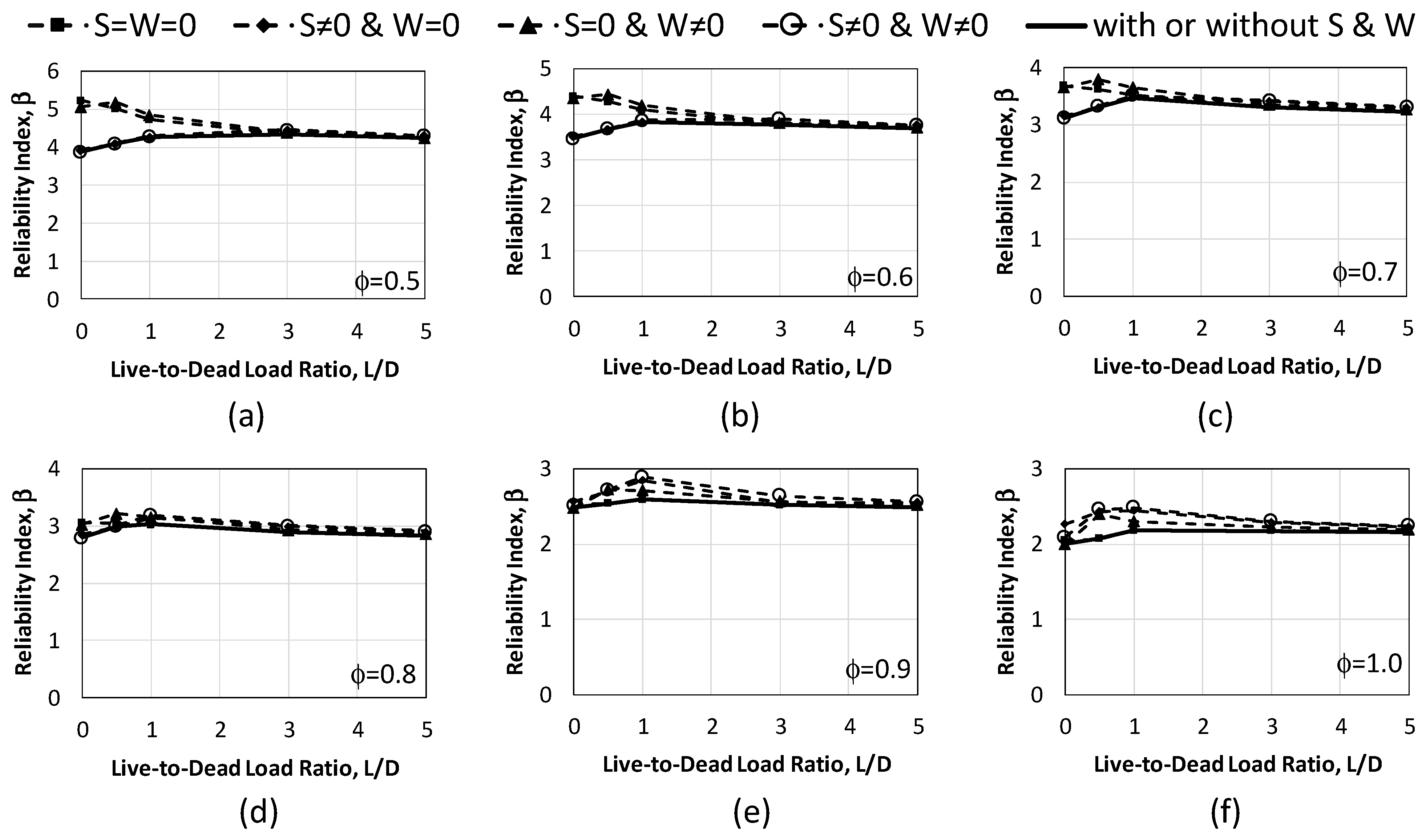
To illustrate the methodology further, we consider an element with lognormally distributed resistance that has a mean-to-nominal ratio of λ
R = 1.2 and a coefficient of variation of V
R = 0.20. The relationships between reliability index and live-to-dead load ratio with and without wind and snow for a set a resistance factors based on the NBC load combinations are presented in
Figure 2. As expected, the reliability index increases with a decrease in the resistance factor, the relationship between the reliability index and load is nonlinear, and the nonuniformity in the latter relationship is particularly obvious for small live load fractions.
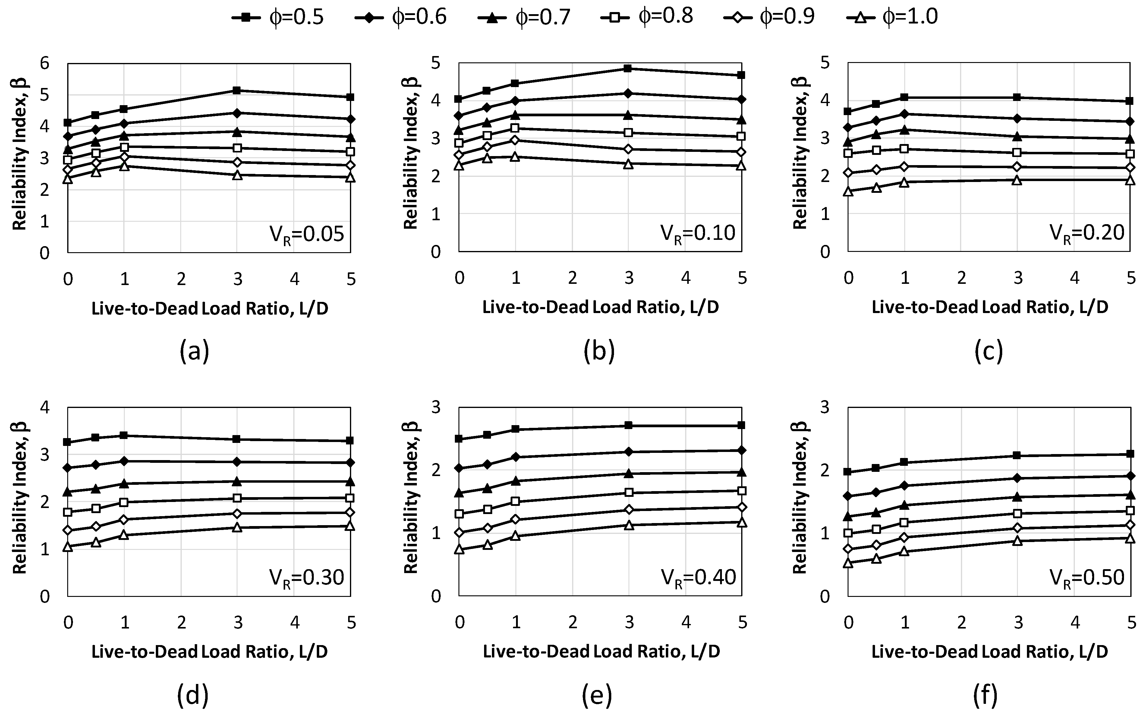
To select an optimum value of a resistance factor for a structure with a resistance represented by given λ
R and V
R, it is best to plot all the relationships between reliability index and loads for a constant resistance factor in one graph, as shown in
Figure 3 for the case of λ
R = 1.2 and V
R = 0.20. This helps in determining which loads and load fractions govern the reliability of the structure, leading to proper selection of the resistance factor. Note that the results in
Figure 2 indicate that while the load combinations involving wind and snow greatly influence the choice of small resistance factor values, such loads are not critical when the resistance factor is large.
The approach outlined in the previous discussion for determining appropriate resistance factors is valid for any combination of λR and VR. Hence, for a study to be useful, it needs to be repeated for a practical range of statistics of the resistance, as presented in the next section.
8. Results
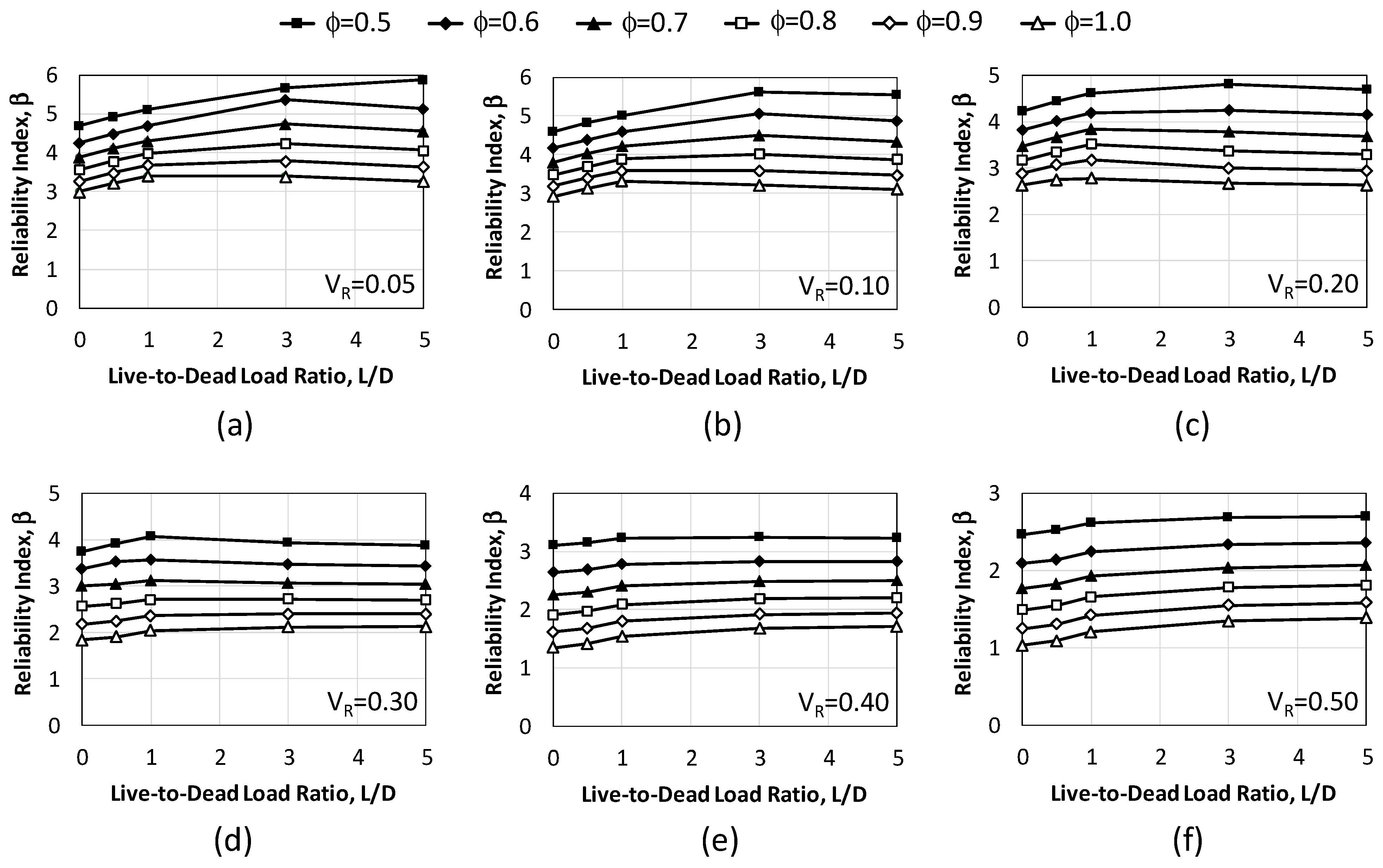
Results of the reliability analyses that were presented in
Figure 3 for the case of λ
R = 1.2 and V
R = 0.20 are now repeated for wide ranges of λ
R (1.0–1.5) and V
R (0.05–0.50), with the probability distribution of the resistance being lognormal. The generated charts, presented in
Figure 4,
Figure 5,
Figure 6,
Figure 7,
Figure 8 and
Figure 9, show the critical reliability indices from the NBC load combinations for a broad spectrum of ϕ (0.5–1.0) with consideration of a practical range of L/D (0–5), S/D (0–2) and W/D (0–2) ratios. This means that, in each chart, the line corresponding to a given resistance factor represents the minimum β for all seven NBC load combinations presented earlier in Equation (6) with consideration of different load fractions. Although the charts only show the L/D ratio along the horizontal axis, each point on the lines shown in the chart corresponding to a given resistance factor considers the effect of presence of wind and snow to different degrees on the reliability.
Besides the obvious finding that the reliability index decreases with an increase in V
R, decrease in λ
R, and/or increase in ϕ, the results provided in
Figure 4,
Figure 5,
Figure 6,
Figure 7,
Figure 8 and
Figure 9 indicate that the reliability index increases with a small increase in live load up until L/D reaches 1.0; thereafter, the shape of the relationship will depend on the resistance’s λ
R and V
R, as well as the value of ϕ. For a small ϕ (<0.8) and V
R (<0.2), β will keep increasing with an increase in the L/D ratio from 1.0 until 3.0, albeit at a lesser rate. For L/D > 3, the relationship between the critical β and applied load is just about constant for designs based on the NBC with a specified value of ϕ. Both λ
R and V
R are equally effective in influencing the structural reliability; however, they work in different ways. The magnitude of λ
R and V
R are impacted by how the close the nominal material properties, cross-section dimensions, and overall geometry are to the average values, as well as how the code’s predictive equations are reliable in forecasting the actual behavior. As such, materials that are manufactured under tight quality control, structures that are constructed within small tolerances, and theoretical formulations that closely forecast the performance at ultimate can economically benefit from small values of λ
R and V
R.
10. Summary and Conclusions
This investigation focused on developing resistance factor spectra for the ultimate limit state of structures and foundations designed following the factored load combinations of the National Building Code (NBC) of Canada. The motivation was to provide a simple approach for researchers with strong backgrounds in their technical field but limited expertise in structural reliability theory and code calibration methods to determine appropriate resistance factors for their findings to be used in practical design. The objectives were to generate comprehensive charts covering a wide range of resistance parameters and factors for the NBC load combinations and determine the sensitivity of the spectra to changes in the bias factor and coefficient of variation of the resistance model.
The study considered dead, live, wind, and snow loads acting on buildings with statistics from the published literature. A probabilistic lognormal model was used for the resistance, with its mean-to-nominal ratio ranging from 1.0 to 1.5 and coefficient of variation from 0.05 to 0.50. The reliability index was computed through an iterative algorithm that approximates the non-normal distributions to equivalent normal ones at the design point. Charts were generated showing the relationship between reliability index and live-to-dead load ratio with different wind and snow load fractions for six resistance factors between 0.5 and 1.0, six mean-to-nominal ratios between 1.0 and 1.5, and six coefficients of variation between 0.05 and 0.50. This covers practical ranges of parameters for structural and geotechnical engineering applications.
The results of the research lead to the following conclusions that are relevant to loads and load combinations addressed by the NBC [
46]:
The reliability indices increase almost linearly with the increase in live-to-dead load ratio until around 1.0, beyond which the relationship becomes nearly nonlinear.
For a small resistance factor and coefficient of variation, the reliability index continues to rise with increase in live-to-dead load fraction from 1.0 to 3.0, but at a lesser rate.
For live-to-dead load fractions above 3.0, the reliability index becomes just about constant irrespective of the magnitude of live load.
The presence of wind and snow loads impacts the choice of an appropriate resistance factor when it is small but does not greatly influence the results when the resistance factor is moderately large to high.
Both the bias factor and coefficient of variation of the resistance are equally effective in changing the structural reliability, albeit through different means.
As expected, structures made from materials that have tighter quality control measures and more precise code equations possess bias factors close to unity with small coefficients of variation, thus allowing for the use of higher resistance factors.
The study successfully met the intended objectives by generating resistance factor spectra charts that can be conveniently used by researchers and code-writing professionals to determine appropriate resistance factors for the Canadian NBC load combinations. The findings provide guidance concerning the sensitivity of the results to changes in the statistical parameters of the resistance model. The provided information will assist designers and code developers in choosing resistance factors that will achieve target reliability indices. The results are particularly beneficial for emerging materials and innovative systems that have been successfully researched but are not yet part of the structural design code.
There are some limitations within the research that need to be highlighted. First, the study considered only the lognormal distribution for the resistance model. While this is the most widely used in practice, results may somewhat vary for other probability distributions. Second, the findings are strictly applicable to design approaches that utilize lumped resistance factors rather than partial factors. Third, the earthquake load effect was not considered in the study due to the lack of reliable probabilistic models for the seismic loading. Finally, the study is limited to the NBC load combinations and does not address other structural design codes. Despite these restrictions, the methodology and outcomes provide a solid platform that can be extended in future investigations.
Recommendations for future work include: (1) Considering other probability distributions for the resistance such as normal, gamma or Weibull; (2) Including other environmental loads that are region-specific, such as earthquake load; (3) Developing user-friendly and interactive software or digital applications based on the results; and (4) Extending the work to cover serviceability and extreme-event limit states.
The resistance factor spectra generated in this study provide researchers and code developers with a simple but rational tool for determining appropriate resistance factors for emerging materials and innovative systems. The findings will contribute towards designing safe and sustainable structures and foundations that utilize such new technologies and construction techniques.


