Determinants of Urban Residential Electricity Consumption in Burkina Faso: A Study of Dwelling, Household, Socio-Economic and Appliance-Related Factors

Abstract

This study analyses the dwelling, household, socio-economic and appliance-related determinants of urban domestic electricity use in Burkina Faso. A survey of 387 households in Ouagadougou was conducted and combined with their electricity use, collected from energy bills. To the authors’ knowledge, this is the first large-scale, city-wide household electricity study undertaken in Burkina Faso. Linear regression models were applied to the data to assess the influence of household, dwelling, socio-economic and appliance-related factors on electricity use. Significant and unambiguous predictors of urban domestic electricity use included household income, dwelling tenure type and ownership, and use of lighting fixtures, television sets, fridges, fans, freezers and air conditioners. Dwelling, household and socio-economic factors explained 70.2% and 70.5% of the variance in electricity use, respectively, when combined with appliance ownership and use factors. This study provides an understanding of the driving factors of domestic electricity use and discusses the implications and applications of this research for a range of stakeholders in the electricity sector.

1. Introduction

Within the building sector, electricity is mainly used to power lighting, appliances and heating, ventilation and air-conditioning (HVAC) systems. Access to such energy is, therefore, considered an essential social and economic need by this sector [1,2]. In Burkina Faso, the residential sector represents 33% of the overall demand for electricity in the country [3,4], making it a crucial target for demand-side management (DSM) and more efficient use of energy. However, accurate information about households’ lifestyles, including socio-economic and dwelling characteristics, appliance ownership and use and factors influencing electricity consumption, which are essential to design effective DSM and energy efficiency programs, remains challenging to find. Contrary to many other countries where residential electricity consumption (REC) has been widely investigated [5,6,7,8,9,10,11], there is a great paucity of information on actual REC in the Global South, and Burkina Faso in particular. REC has been investigated in only a few countries in Sub-Saharan Africa, including mainly South Africa [12,13,14], Ghana [15,16,17,18] and Nigeria [19]. In Burkina Faso, the paucity of studies is even more significant. Apart from studies by the National Institute of Statistics (INSD/BF) on the living conditions of the population, which gathers some data on household energy expenditure, and a recently published study by the current authors analysing how households’ lifestyles and behaviours relate to the level of electricity use in urban domestic residential buildings [20], almost no studies on REC exist. There is, however, a great interest by the country’s government in improving electricity use. In 2016, the National Agency for Renewable Energy and Energy Efficiency (ANEREE) was created to foster the development of renewable energy and energy efficiency in Burkina Faso. In addition, among the grid operators and utility companies, having accurate information on the details on electrical energy end uses, in addition to the factors that influence the dynamics of residential electricity use, is essential for sound management of the country’s electricity system and providing good quality services to users [17]. Finally, there is interest from the country and regions’ energy research community as accurate information is essential for them, in order to assist the authorities in setting up strategies and policies for DSM or energy efficiency.

This study aims to improve the weak literature on REC in Burkina Faso by providing insights into the determinants of electricity consumption within urban households. For this purpose, this study uses the data collected from a residential electricity consumption survey (RECS) of 387 households in the city of Ouagadougou, which, to the authors’ knowledge, is the first large-scale, city-wide household electricity study undertaken in Burkina Faso. As mentioned previously, the first study by the authors [20] uses the results from the study to present an initial overview of the socio-economic background of urban households in Burkina Faso, as well as their level of electricity consumption and related activities and behaviours. This study steps beyond the previous one, by trying to identify the factors that influence such electricity use. More specifically, the present study developed quantitative multivariate models of dwellings, households, and socio-economic factors and appliance ownership and use factors in relation to urban REC in Burkina Faso, to address the following questions: What are the main direct (factors that imply the direct use of electricity: number, daily time of use of appliances and the energy behaviours of users towards appliances and electricity) and indirect (factors that indirectly imply the use of electricity and factors that influence the use of lighting and appliances) determinants of electricity consumption within urban households in Burkina Faso? How can electricity consumption within urban households in Burkina Faso be predicted using such factors? How much variance in electricity consumption do these factors explain? What are the policy implications and applications of this research for stakeholders in the electricity sector?

In the rest of the paper, Section 2 presents the research methodology for conducting this study. Section 3 presents and discusses the results, as well as the policy implications. Finally, Section 4 summarises the study’s findings and concludes the paper.

2. Literature Review

Determinants of REC have been widely investigated across the world. The most common approaches used to establish them include statistical, regression and probabilistic techniques, depending on the type of data collected and level of investigation [21]. At the macro level, high-level data are collected, such as demographics, housing statistics and gross domestic product (GDP), and “top-down” approaches are used to derive the causal relationships between these factors and electricity consumption [21,22]. At the micro level, “bottom-up” models are used instead, with data collected at an individual level, in order to determine the causal relationships between the household-level factors and electricity consumption [21,23]. In the current study, attention is paid exclusively to investigations at the micro level using bottom-up models. Therefore, the determinants discussed in this section encompass only household-level driving factors of electricity use, including not only socio-economic and dwelling factors, but also behavioural, technical and appliance-related factors.

2.1. Socio-Economic and Household Factors

The main socio-economic and household driving factors of electricity use investigated in the REC literature include family composition, tenure type, household income, disposable income, household size (number of occupants) and characteristics of the household responsible person (HRP) like age, education level and socio-economic classification [24]. Within such factors, the household size, presence of teenagers, and household and disposable income were found to be unambiguously significantly and positively correlated with electricity use [24].

For example, Sakah et al. [17] made use of a multiple linear regression (MLR) method to analyse questionnaire and monitoring data within 60 urban Ghanian households and found that socio-economic, dwelling, appliance-related and energy behaviour factors explained 56.8% of the variance in electricity consumption. More specifically, household size and income were found, within the socio-economic factors, to be significantly and positively correlated with electricity use, with a one unit rise in these factors leading to an annual increase in electricity use of 580.3 and 2 kWh, respectively. Using logit regression analysis consisting of OLS regression models built upon the Irish Household Budget Survey (HBS) dataset, Leahy and Lyons [25] calculated that an increase in the log of household disposable income by one unit, increased electricity use by 4% per week.

Previous investigations on the influence of family composition on electricity use found that the presence of teenagers was significantly and positively correlated with electricity use [26,27,28]. For example, Bartusch et al. [28] explored the variation in electricity use within Swedish households using statistical approaches, including independent samples t-tests and one-way and univariate independent samples analyses of variance. They found significantly higher annual electricity consumption per m² of electrically heated living space for families with teenagers in Sweden.

Tenure type and characteristics of the HRP have also been widely investigated [17,23,25,29,30,31,32] and found to have significant effects on electricity use. However, as such factors are investigated using categorical variables, it is not possible to establish a positive or negative correlation with residential electricity use [24]. Furthermore, the age of the HRP has been found to have a significant effect on the electricity consumption in residential buildings [24].

2.2. Dwelling Factors

The main dwelling-related driving factors of electricity use investigated in the REC literature include not only the dwelling type, age and size (floor area or number of rooms), but also the presence in the dwelling of householders and systems like HVAC, DHW and efficient lighting [24]. Dwelling size and age and the presence of air conditioning, electric space heating and water heating systems have been identified as unambiguously, significantly and positively correlated with REC in the literature [24].

For example, Sakah et al. [17] found a positive relationship between the total floor area and electricity use within Ghanaian households, with a recorded increase in annual electricity use by 7.1 kWh for each 1 m² increase in floor area. Floor area was also found as significant and positively correlated with REC by Kavousian et al. [32], who used weighted regression models to examine the structural and behavioural determinants of US domestic electricity consumption using a dataset from 1628 households.

Regarding the number of rooms/bedrooms in the dwellings, Bedir et al. [29] used the data collected through a survey of 323 Dutch households and developed three combined regression models, incorporating direct (appliances factors) and indirect (household and dwelling factors) determinants of electricity use and found that the number of rooms, and particularly the number of study/hobby rooms, was positively correlated with electricity consumption.

Dwelling age, which is commonly treated as a categorical variable, also demonstrated an unambiguously positive relationship with REC, meaning that the older the dwelling, the greater the amount of electricity it uses. For example, Leahy and Lyons [25] demonstrated that Irish homes built before 1918 used significantly more electricity per week (6.1%) than those built between 1918 and 1960. Such an increase was explained as resulting from an increase in heat loss associated with less insulation and the use of electric heating and power showers instead of gas. They also found that households built later than 2000 used significantly less electricity than dwellings built in 1918–1960.

2.3. Appliance Factors

The appliance-related driving factors of electricity use investigated in the literature consists of two main parts: ownership and use. The literature clearly demonstrates that the total number of appliances owned, ownership of particular appliances like desktop computers, televisions, electric ovens, fridges, dishwashers, and tumble dryers, and the use of some major appliances like washing machines and tumble dryers, significantly increase residential electricity usage [24].

For example, the number of electric appliances was found to be positively and significantly correlated with electricity use by Danlami [19], who used an OLS regression model to examine electricity use in Nigerian households. Similarly, using MLR analysis of annual electricity consumption by Japanese households, Genjo et al. [9] calculated that a one unit increase in appliance stock significantly increased the annual electricity use by 62 kWh. For Ghanian households, Sakah et al. [17] found that the ownership of a television and refrigerator significantly and positively correlated with electricity use; more specifically, they calculated an increase in the annual electricity use of 226 kWh and 127 kWh for each additional refrigerator and television owned. McLoughlin et al. [31] found that dishwashers, tumble dryers and desktop computers were the appliances that consumed the most electricity in Irish dwellings and were significantly and positively correlated with REC.

However, a part of the literature on REC considers that the number of appliances alone only partially reflects their effect on residential electricity use, which makes it necessary to consider their frequency of use instead [33]. Few pieces of research exist on the influence of appliance use on REC [26,29,31]. For example, the duration of the use of appliances, including information, communication, entertainment, HVAC, washing and laundry appliances were found to explain 37% of the variance in electricity consumption within Dutch households by Bedir et al. [29]. Similarly, Bartiaux and Gram-Hanssen found a significantly positive correlation between the duration and frequency of use of washing appliances and electricity demand in Dutch households [26].

2.4. Other Factors

Various other factors have also been reported in the existing literature, including electricity price, location, ownership of specific systems, activities and energy behaviours of the occupants. For example, Sakah et al. [17] established that awareness and practice of energy conservation can significantly help to decrease annual electricity use by 1277 kWh within urban Ghanian households, while McLoughlin et al. [31] found significantly higher electricity consumption by Irish households who believe they can cut their annual electricity use by high percentages (10–30%). Using a general linear regression model (GLM), Fan et al. [34] identified that the ownership of a swimming pool was found to be one of the significant predictors of Australian residential peak electricity demand. The price of electricity was investigated by O’Doherty et al. [22], who found a 2.1% increase in energy use due to off-peak electricity tariffs.

2.5. Summary of Previous Literature Methods and Results

The existing body of literature suggests that a large range of factors, including socio-economic and household, dwelling, behavioural, appliance-related and other factors, are related to REC. Based on the reviewed literature, statistical analysis and, more specifically, regression analyses, were mostly used by studies dealing with sizeable datasets to provide insights into the determinants of residential electricity use [17]. The major drawback of such studies is the high possible cost of implementation and issues concerning multicollinearity between variables [21].

The current study has used a statistical approach based on a multiple linear regression model to analyse the underlying factors of variations in urban REC in Burkina Faso. The recorded annual electricity consumption of households was used as the dependent variable, whereas household, dwelling, socio-economic and appliance-related factors obtained from a household survey were used as independent variables.

3. Materials and Methods

3.1. Study Area

In Burkina Faso, only 5.9% of the rural population have access to electricity, while at the same time, the urban population, which represents only 26.4% of the total population, have access to electricity services at a rate of 72.5% and use 74% of the total electricity used in the country [35]. The urban areas were, therefore, chosen for our study as they represent a large amount of the total electricity used in the country. Moreover, the city of Ouagadougou (Figure 1) was selected due to its representativeness of the urban areas. Ouagadougou, which is located in the central region of Burkina Faso, is the capital and largest city. With a total population of 2,453,496 inhabitants, the city consists of 12 districts and 55 sectors, and alone represents 45.4% of the country’s urban population [36]. The location of Ouagadougou, at longitude 01°31′05″ W and latitude 12°21′58″ N [37], places it in the Sudano-Sahelian climatic zone, conferring the climate with a dry and hot character. Mean monthly temperatures range from 33 °C during the dry and hot seasons (March to June and November), to 25 °C during the dry and cold seasons (December to February) [38]. During the rainy season (July to October), the rainfall reaches up to 200 mm, while the mean relative humidity is estimated as 48.5%. The city was, therefore, chosen because it is a good representant of the urban areas in Burkina Faso. Also, the findings on the city can be used as reference points for predicting the REC in the other urban areas of Burkina Faso.

3.2. Design of the Survey and Data Collected

3.2.1. Size of the Studied Sample

In order to make a compromise in the study between accuracy and the available resources, not all the population of the households in Ouagadougou were studied. Instead, sampling was adopted (with the “stratified” random sampling technique used, as the city consists of 12 districts). Indeed, such an approach is known for its numerous advantages, with respect to complete enumeration including reduced cost, greater speed, greater scope and greater accuracy [40]. The sample size was calculated, as suggested by Cochran [40]. Such approach is recognised as not only useful for either research experiments or surveys [41], but it is also flexible when using various types of information (size, proportions or statistics) on the target population [41,42]. Furthermore, it is commonly used in the surveys in the literature, including those on domestic electricity use [19,43,44]. The sample size is given here in its decomposed form by Equations (1) and (2).

$${\mathbf{n}}_0={\mathbf{z}}^2\mathbf{p}\mathbf{q}/{\mathbf{e}}^2$$

(1)

$$\mathbf{n}={\mathbf{n}}_{\mathbf{o}}/(1+(\left({\mathbf{n}}_0-1\right)/\mathbf{N}\left)\right)$$

(2)

In Equation (1), ${\mathbf{n}}_0$ refers to the non-adjusted sample size, i.e., the sample size for an infinite and unknown population size, z represents the z-score corresponding to the chosen confidence interval, p refers to a proportion of the population which has a defined attribute, q = 1 − p and e is the margin of error. When the size of the target population, which is N here (the number of households in Ouagadougou), is known, a correction factor is introduced by Cochran [40], therefore, Equation (2) is used to correct the sample size. The adjusted/corrected survey sample size (n) was, therefore, determined in our study as 384, which is at a 95% confidence interval, with a proportion of 50% and a 5% margin of error (e).

3.2.2. Investigation Methods and Results of the Survey

Data was collected during the survey by means of questionnaires sheets, which are known for their suitability regarding data gathering [45]. Moreover, they are often used in studies on energy consumption [46]. Considering the structure of the city of Ouagadougou, 12 districts and 55 sectors, the sample size consisted of a combination of the sample sizes of the districts, with a proportional relationship established between the number of selected households and the total number of households in each district.

Random sampling was used as the household selection method throughout the survey, in order to make sure that each household had an equal chance of being selected. However, household participation also depended on their readiness and willingness to participate (Figure 2). Finally, attention was also paid to the selection of households with different backgrounds and economic levels throughout the sampling process.

Table 1. Authors’ contributions to the elaboration and implementation of the survey.

Stage	Activities and Authors Involved
Survey Design	Conception	Validation	Obtaining necessary approbations
	Author 1 Author 2 Author 3	Author 2 Author 5 Author 4	Author 1 Author 2
Survey Test	Author 1, Author 3
Survey Implementation	Questionnaire distribution and recovery		Other complementary data collected
	Author 1, Author 3, Author 5, Author 2		Author 1

shows the role of the authors in the survey design and implementation. The name of the authors has not been given, instead, a number has been given to them according to their order of appearance on the title page.

Finally,

Table 2. Ouagadougou’s structure and number of participants per district.

N° District	Area (km2)	Population Size	Number of Households	People per Household	Surveyed Households	People per Surveyed Household
1	18.65	102,016	25,771	4.0	23	6.0
2	12.70	83,436	20,203	4.1	23	4.8
3	60.56	311,406	66,595	4.7	56	5.0
4	82.81	207,647	49,088	4.2	36	6.0
5	21.40	129,984	33,115	3.9	28	5.3
6	29.00	222,854	49,619	4.5	39	6.5
7	32.68	282,837	70,180	4.0	32	5.5
8	66.57	152,880	36,098	4.2	15	4.9
9	88.27	336,483	79,889	4.2	34	3.9
10	27.96	263,969	63,579	4.1	45	4.9
11	48.30	254,928	62,221	4.1	44	5.8
12	44.13	66,826	15,811	4.2	12	6.2
Total	533.03	2,415,266	572,169	4.2	387	5.4

provides the characteristics and number of surveyed households for each district in this study. From such a table, it can be noticed that except for district 9, the number of people per household in each district, from the results in this study, is slightly higher than that from the results of the last census of the country (RGPH, 2019) [36].

3.2.3. Ethical Considerations in the Data Gathering Process

Ethical considerations related to the data gathering process concerned mainly the participants in the survey. First, the current study is part of a research programme that has been designed and approved according to the research direction of the host institute (2iE Institute) after several screenings by various departments, including the deontology and ethics committee (N°2023/01/DG/SG/DR/HK/fg). In addition, a specific approbation for the implementation of the survey was received by the authors according to the research direction of the host institute. Such an approbation was subject to the following considerations: presentation of an invitation letter to the participants (signed by the Research Director), presentation of an information sheet to the participants (description of the content, scope and objectives of the survey), obtaining permission from the participants, presentation of ID of the host institute to the participants by the researchers before starting the interviews, keeping confidential all data and securely storing the personal data of the participants.

3.2.4. Data Collected

The survey content is shown in

Table 3. Items covered by the survey.

Items Investigated	Content or Description
Electricity use	Monthly electricity consumption (amount and cost from bills), electricity sources and electricity account information.
Appliance ownership and use	Appliance stock characteristics (type and number of appliances), appliance purchase condition, typical days appliance pattern of use (weekdays/weekends).
Dwelling characteristics	Tenure type, building’s period of construction and type, floor area, number and role of rooms, number of storeys and presence of HVAC/DHW systems.
Household characteristics	Household size, family status, member’s age and relation to the household responsible person (HRP), education level, monthly income, employment status of the HRP.
Daily life activities	Household daily life activities involving the presence and use of appliances in dwellings.
Energy behaviour	Appliance labelling awareness and influence on purchase, energy conservation awareness and practices, standby consumption awareness and behaviours.
Others	Preferred appliances for load shifting and curtailment to avoid power outages. Level of satisfaction regarding utility services, etc.

. As can be seen, the survey content was designed around domestic residential electricity use and items characterising household behaviours and lifestyles. Such items were demonstrated to be linked to electricity use in the literature on domestic REC. A household’s annual electricity consumption was recorded from the household’s electricity bills. The electricity bills were collected for the year 2021 and were used to compute the annual electricity use of the participants.

Table A4. Characteristics of the appliance stock (number) in the households investigated in the study.

Appliance Ownership	Minimum	Mean	Maximum	Std. Dev
Indoor lighting	1	8.70	40	5.96
Outdoor lighting	0	2.51	12	1.85
Fan	0	4.34	24	3.03
Television	0	1.39	8	0.89
Satellite receiver	0	1.12	8	0.80
Fridge	0	0.93	4	0.66
Laptop	0	0.96	8	1.17
Air conditioner	0	0.63	9	1.23
Iron	0	0.30	3	0.51
Radio	0	0.23	3	0.49
Sound system	0	0.21	4	0.49
Blender	0	0.18	2	0.39
Microwave/oven	0	0.19	2	0.43
Freezer	0	0.17	2	0.41
Desktop computer	0	0.17	4	0.49
Kettle	0	0.12	3	0.34
Wi-Fi router	0	0.10	3	0.32
Games console	0	0.10	3	0.36
DVD/VCR player	0	0.08	2	0.31
Printing machine	0	0.04	2	0.20
Humidifier	0	0.03	1	0.17
Washing machine	0	0.03	1	0.16
Electric stove	0	0.04	6	0.34
Others *	0	0.04	3	0.25

* Other devices else than common domestic appliances including working machines (tailoring machines, wood piercer), sports devices, electronic pianos etc.

,

Table A5. Nominal power of the investigated appliances.

Name of the Appliance	Options	Unitary Power of Use (W)	Unitary Standby Power (W)
Television	Screen size ≤ 32″	52	8
	32″ < Screen size ≤ 40″	93	8
	40″ < Screen size ≤ 65″	125	5
	Screen size > 40″	196	5
Satellite receiver	Type 1	18	16
	Type 2	20	4
	Type 3	6	0.15
Ballast fluorescent lighting fixtures	0.6 m	25	-
	1.2 m	45	-
Compact fluorescent lighting fixtures	-	28	-
LED lighting fixtures	0.6 m	9	-
	1.2 m	18	-
	Bulb	15	-
Other lighting fixtures	-	75	-
Fridge	Capacity ≤ 100 L	64	0.6
	100 L < capacity ≤ 200 L	96	0.6
	100 L < capacity ≤ 300 L	111	1.0
	Capacity > 300 L	121	1.0
Freezer	Capacity ≤ 100 L	68	0.6
	100 L < capacity ≤ 200 L	125	1.0
	100 L < capacity ≤ 300 L	162	1.0
	Capacity > 300 L	305	1.0
Fan	Ceiling	42–70 *	-
	Movable	42	-
Air conditioner	Type 1	656	-
	Type 2	921	-
	Type 3	1302	-
	Type 4	1828	-
	Type 5	2220	-
Desktop computer	-	200	25
Laptop	-	60	2
Radio	-	15	6
DVD/VCR	-	43	4
Sound system	-	57	8
Wi-Fi router	-	11	5
Games console	-	150	7
Printing machine	-	400	10
Iron	-	200	-
Blender	-	125	-
Kettle	-	1500	2
Humidifier	-	150	-
Microwave/oven	-	980	1
Washing Machine	-	800	3
Electric stove	-	1500	-

* Depends on the speed at which the fan is used.

and

Table A6. Descriptive statistics on the recorded electricity consumption.

Statistics	Recorded Annual Electricity Consumption (kWh)
Mean	2395
Standard deviation	1687
Minimum	181
Maximum	10,188

show the characteristics of the appliance stock of the participants, as well as that of their recorded annual electricity use.

3.3. Data Processing and Analysis

The data processing framework is outlined in Figure 3. Based on the literature review, data were collected on numerous factors (

Table A1. Dwelling, household and socio-economic (DHSE) factors included in the study.

Group of Factors	Variable (Factor/Predictor)	Variable Type	Measurement/Options
Dwelling, Household and socio-economic (DHSE) characteristics	Family composition	Categorical	Single/couple/couple with non-dependent children/family with non-dependent children/couple with dependent children/single-parent family/family with dependent children/other
	Household size	Continuous	Number of people in the house
	Household income (monthly): in USD	Categorical	Class G (up to 168)/class F (168–419)/class E (419–671)/class D 671–923/class C (923–1175)/class B (1175–1426)/class A (1426 and more)
	HRP age	Categorical	Up to 28 years old/29–39 years old/40–50 years old/51–61 years old/62 and more years old
	HRP employment status	Categorical	Unemployed/retired/part-time employee/own business/full-time employee
	HRP education level	Categorical	Never attended school/primary school/secondary school/university/college
	HRP socio-economic category	Categorical	Unskilled and agricultural worker/manual-skilled or semi-skilled worker/non-manual worker/business owner/managers and professionals/other
	Gender of HRP	Dummy	Male/female
	Marital status of HRP	Dummy	Married/not married
	Number of active people	Continuous	Number of people working and earning
	Presence of teens	Dummy	Yes/no
	Presence of children (0–12 YO)	Dummy	Yes/no
	Presence of elders/retirees	Dummy	Yes/no
	Presence of housewife	Dummy	Yes/no
	Floor area	Continuous	Floor area in square meters
	Dwelling period of construction	Categorical	Until 1970/1970–1980/1980–1990/1990–2000/after 2000
	Dwelling type of construction	Categorical	Multi-family house/apartment block/semi-detached house/detached house
	Dwelling tenure type	Categorical	Free rented/privately rented/owner occupied
	Dwelling number of storeys	Continuous	Number of storeys in the dwelling
	Dwelling number of rooms	Continuous	Number of rooms in the dwelling
	Dwelling number of bedrooms	Continuous	Number of bedrooms in the dwelling
	Dwelling number of other rooms	Continuous	Number of rooms used for other purposes (other than the living room and bedrooms)
	Presence of a HVAC system	Dummy	Yes/no
	Presence of a DHW system	Dummy	Yes/no
	Overall presence in the living room	Continuous	Duration (hours) of the presence of people in the living room in 24 h
	Daytime presence in the living room	Continuous	Duration (hours) of the presence of people in the living room from 8:00 a.m. to 5:00 p.m.
	Overall presence in the bedrooms	Continuous	Duration (hours) of the presence of people in the bedrooms in 24 h
	Other presence in the bedrooms	Continuous	Duration (hours) of the presence of people in the bedrooms for activities other than resting

,

Table A2. Appliance ownership (AO) and appliance use, and energy behaviour (AUEB) factors, included in the study.

Group of Factors	Variable (Factor/Predictor)	Variable Type	Measurement/Options
Appliance ownership	Ownership of a Y * type appliance	Continuous	Number of the Y type appliance in the house
Appliance use and energy behaviour	Use of a Y * type appliance	Continuous	Daily duration of use of the Y type appliance (hour)
	Appliance purchase condition	Categorical	New/second hand/mixed
	Awareness of appliance labelling	Dummy	Yes/no
	Influence of label on appliance purchase	Dummy	Yes/no
	Practice of energy conservation	Categorical	Yes/no/sometimes or not really
	Energy conservation actions	Categorical	Turn off unused/turn off and unplug unused/usage of efficient light/ usage of solar PV system/none
	Awareness of standby consumption	Dummy	Yes/no
	Ownership of standby appliances	Continuous	Number of standby mode appliances
	Unplugging standby mode appliances	Categorical	Yes/no/sometimes or not really
	Satisfaction related to utility services	Categorical	Not at all/not really/neutral/more or less/yes/yes, very
	Appliance preference for load shifting	Categorical	Fan/fridge or freezer/air conditioner/TV set/others

* Corresponds to the appliances that were found in the households (see Table A2).

and

Table A3. Activities of the households and corresponding appliances investigated in the study.

Activity	Appliances
Cooling	Humidifier, fan, air conditioner
Cooking/food preserving	Freezer, fridge, blender, kettle, microwave/oven, electric stove
ICE	Television, satellite receiver, sound system, games console, Wi-Fi router, desktop, laptop, radio, DVD/VCD, printing/scanning machine
Lighting	Indoor and outdoor lighting fixtures
Others	Washing machine, iron, others

) due to their demonstrated effect on REC. An analysis of the correlations (using Pearson’s r) helped reduce the number of predictors by retaining only the significantly correlated factors to REC, for the next step in the analysis. In the next step of the analysis, the retained factors were entered into multiple linear regression (MLR) models to find the significant predictors of REC and the amount of variance in the REC explained by such predictors.

Simple regression models were used first, using a stepwise method [23] to find the significant predictors of REC for each category of factors, including not only direct effect factors, namely appliance ownership (AO) factors (model A), and appliance use and energy behaviour (AUEB) factors (model C), but also indirect effect factors, namely dwelling, household and socio-economic (DHSE) variables (model B). Following this, the identified significant predictors of the three defined categories (A, B and C) were introduced into two combined regression models. The first combined model (I) used DHSE and AO factors that were found to be significant in the previous simple models (A and B), while the second model (II) used DHSE and AUEB factors (B and C). The two combined models were built separately to provide more insights into the effect of appliance ownership and use, and the amount of variation in the REC that they can explain when investigated separately. This aspect was undertaken as the existing literature lacks comparative studies on these two elements.

The MLR function helps evaluate the linear relationship between a dependent variable (Y) and several independent variables or functions of independent variables (X) [17]. Linear regression estimates how much Y changes when X changes by one unit. The MLR function is presented by Equation (3):

$$\mathbf{Y}={\mathsf{\beta }}_0+{\mathsf{\beta }}_1{\mathbf{X}}_1+{\mathsf{\beta }}_2{\mathbf{X}}_2+\dots +{\mathsf{\beta }}_{\mathbf{n}}{\mathbf{X}}_{\mathbf{n}}+\mathsf{\epsilon }$$

(3)

where Y is the dependent variable (the log of REC was used in our study as the dependent variable), and ${\mathbf{X}}_{1\dots \mathbf{n}}$, the independent or explanatory variables, i.e., here DHSE, AO and AUEB variables. Moreover, ${\mathsf{\beta }}_0$ stands for the intercept (or constant), i.e., the value of Y when the values of all the explanatory variables are 0, while ${\mathsf{\beta }}_{1\dots \mathbf{n}}$ represent the regression coefficients. Here, they reflect the magnitude and direction of change in the REC in a household when the degree of a predictor increases by one unit, while holding all the others constant. A negative coefficient indicates a reduction in the REC, while a positive coefficient indicates an increase in the REC. Additionally, $\mathsf{\epsilon }$ is the random error term, which measures how far above or below the true regression line (i.e., the line of means) the actual observation on Y lies [17].

The ordinary least squares (OLS) method was used to estimate all the regression coefficients in the model. The proportion of variance in the dependent variable that is predictable from the independent variables is estimated using the coefficient of determination (R²), which shows how well the values fit the data and is used as a guideline to measure the model’s accuracy [47]. The SPSS software (IBM SPSS Statistics 20) was used to perform all the statistical data processing, treatment and analysis.

4. Results

4.1. Preliminary Analyses

Before the models were run, the preliminary assumptions of the linear regression model were checked for each model (A–C, I and II), including the additivity, linearity, normality, homogeneity of variance (homoscedasticity) and independence of the dependent variable. Also, the correlations between the independent variables and the dependent variable (residential electricity consumption: REC) were checked. Finally, other checks such as multicollinearity check between the variables and the influencing observations (outliers) were also run.

4.1.1. Preliminary Assumptions Checking

The additivity, linearity and homoscedasticity were checked together. All of these elements can be assessed using a single graph, as they are all related to errors (or residuals). A scatterplot, which displays the values of these residuals against the corresponding values in the outcome predicted by the regression model [48] in a graph, was used (see the example for the model B in Figure A1. Normality was also checked using graphs [48] (Figure A2), namely the P–P plot (probability–probability plot) was used, which plots the cumulative probability of a variable against the cumulative probability of normal distribution.

Finally, the presence of outliers was checked using both graphs and numbers. The screening of the scatterplot showed the presence of two particular individuals (Figure A1). Further investigations were conducted, including the use of Cook’s distance, as well as the converted normal z-scores of the REC for the individuals. For Cook’s distance, the maximum distance recorded for all models was 0.182, which is much less than 1, indicating that there was no need to worry about the two individuals [48,49]. The sorting of the converted z-scores of the REC (ignoring whether they are positive or negative) for the individuals indicated that no values were larger than 3.29, only 2% of the values were larger than 1.96 and 0.3% were larger than 2.58. Therefore, no observations violated the outliers’ conditions [48] and, consequently, all the observations were included in the following analyses.

4.1.2. Correlation Checking and Variables Retained for the Analyses

Following the assumption checking for the linear regression models, the next step in the data treatment was to find the correlations between the REC and the variables selected from the literature as potential determinants.

Table A7. AO and AUEB variables retained from the correlation analysis.

Variables	Pearson’s r with REC	Variables	Pearson’s r with REC
Ownership of lighting	0.7 ***	Ownership of freezer	0.4 ***
Ownership of TV set	0.5 ***	Ownership of kettle	0.3 ***
Ownership of desktop computer	0.3 ***	Ownership of blender	0.3 ***
Ownership of laptop	0.4 ***	Ownership of microwave/oven	0.5 ***
Ownership of radio	0.1 **	Ownership of iron	0.3 ***
Ownership of DVD/VCR	0.2 ***	Ownership of washing machine	0.2 ***
Ownership of sound system	0.2 ***	Ownership of electric stove	0.1 **
Ownership of games console	0.3 ***	Ownership of air conditioner	0.6 ***
Ownership of Wi-Fi router	0.3 ***	Ownership of fan	0.7 ***
Ownership of printing machine	0.3 ***	Ownership of other appliances	0.1 **
Ownership of fridge	0.5 ***
Use of lighting	0.7 ***	Use of iron	0.1 **
Use of TV set	0.5 ***	Use of washing machine	0.2 **
Use of desktop computer	0.2 ***	Use of electric stove	0.2 **
Use of laptop	0.4 ***	Use of air conditioner	0.6 ***
Use of radio	0.2 **	Use of fan	0.5 **
Use of sound system	0.2 ***	Practice of energy conservation	0.2 ***
Use of games console	0.3 ***	Energy conservation actions	−0.1 *
Use of Wi-Fi routers	0.4 ***	Appliance preference for load shifting	0.1 *
Use of printing machine	0.2 ***	Awareness of standby consumption	−0.2 ***
Use of fridge	0.6 ***	Ownership of standby mode appliances	0.6 ***
Use of freezer	0.4 ***	Unplugging of standby mode appliances	0.3 ***
Use of kettle	0.2 ***	Use of microwave/oven	0.2 ***
Use of blender	0.3 ***

* p < 0.05, ** p < 0.01, *** p < 0.001.

and

Table A8. DHSE factors retained from the correlation analysis.

Variables	Pearson’s r with REC	Variables	Pearson’s r with REC
Household size	0.3 ***	Number of floors in the dwelling	0.4 ***
Family composition	0.3 ***	Floor area	0.6 ***
Presence of teens	−0.3 ***	Presence of a hot water system	−0.1 **
Presence of elders/retirees	−0.2 **	Presence of a HVAC system	−0.2 **
HRP education level	0.2 ***	Household income	0.7 **
HRP marital status	−0.2 ***	HRP age	0.3 **
HRP socio-economic category	0.2 **	Daytime presence in the living room	0.3 ***
Number of active people in the house	0.3 ***	Overall presence in the bedrooms	0.4 ***
Dwelling tenure type	0.4 ***	Other presence in the bedrooms	0.3 ***
Dwelling construction type	0.4 ***

** p < 0.01, *** p < 0.001.

present the variables retained for the analyses using the regression models (due to the significant correlations existing between them and REC).

Regarding the AO variables (Table A7), previously identified variables affecting REC, like the ownership of fridges, television sets, desktop computers and large appliances like washing machines, were significantly correlated with REC. Furthermore, the ownership of other appliances, such as fans, air conditioners, laptops and lighting fixtures, were also significantly correlated with REC. Finally, rare factors like the ownership of a printing machine, blender and Wi-Fi routers, were also significant and, therefore, included in the regression analyses.

Regarding the AUEB variables (Table A7), it was evident that appliance use factors were also significant for almost all the appliances where ownership was found to be significant. Furthermore, the energy behaviour factors like energy conservation practices, awareness of standby consumption, number and unplugging of standby devices, appliance purchase and appliance preferences for load shifting during peak demand periods, were significantly correlated with REC. Therefore, they were included in regression model C.

Finally, for the DHSE variables, the common variables in the literature, such as household size, floor area, household income, tenure type, age, education level and socio-economic class of the HRP, were significantly correlated with REC (Table A8). Furthermore, other previously identified variables, such as the type of construction, the number of floors in the dwelling and the individuals’ presence in regard to the rooms, were also significantly correlated with REC. Finally, rarely established variables, such as the marital status of the HRP, which has only previously been found in one other Global South study [19], were also significantly correlated with REC. These variables were then entered into the regression model (model B).

Variables not found to be significantly correlated with REC were omitted in the following analyses. For the multicollinearity check, the correlations between the independent variables were investigated, and the values of the coefficients (Pearson’s r) reached up to 0.8, suggesting in some cases that there were some issues. In order to go further, the VIF (variance inflation factor) and the tolerance were computed using SPSS to investigate further the relationship between the predictors. The maximum VIF for all models was 4.86, found in model C, which is less than 10, and the minimum tolerance was found to be 0.21, also in model C, and which again is more than 0.1, indicating no concerns related to multicollinearity [48,49].

4.2. Individual Effect of Factors on Residential Electricity Use: Simple Regression Models (A–C)

4.2.1. Individual Effect of Appliance Ownership on Residential Electricity Use: Model A

Table 4. Regression results for the AO determinants (Model A): significant predictors and their effect on REC.

Variables	B	Std. Error	Β (Beta)
(Constant)	6.578	0.055	-
Ownership of lighting	0.023	0.005	0.241 ***
Ownership of TV sets	0.037	0.018	0.080 *
Ownership of a fridge	0.222	0.039	0.201 ***
Ownership of a freezer	0.295	0.064	0.165 ***
Ownership of a microwave/oven	0.146	0.068	0.087 *
Ownership of an iron	0.120	0.052	0.083 *
Ownership of air conditioning	0.089	0.030	0.150 **
Ownership of a fan	0.055	0.012	0.229 ***

R² = 0.656. * p < 0.05, ** p < 0.01, *** p < 0.001.

shows the results from the first model on the individual effect of the AO factors on REC. The model (A) was run using all the retained variables (from Table A7) to establish the significant predictors of residential electricity consumption (REC). The significant predictors (at least at the 5% level) of REC included here were the ownership of lighting fixtures, TV sets, fans, fridges, freezers, air conditioners, irons and microwaves. The AO factors explained 65.6% of the variance in the REC.

4.2.2. Individual Effect of Dwelling, Household and Socio-Economic Factors on Residential Electricity Use: Model B

The results from the second model, analysing the determinants of REC concerning the DHSE factors, are presented in

Table 5. Regression results for the DHSE determinants (Model B): significant predictors and their effect on REC.

Variables	B	Std. Error	Β (Beta)
(Constant)	5.047	0.231	-
Total floor area	0.002	0.001	0.202 ***
HRP education level	0.086	0.025	0.120 **
Dwelling tenure type	0.215	0.055	0.159 ***
Household income	0.201	0.019	0.461 ***
Daytime presence in the living room	0.025	0.009	0.098 **
Overall presence in the bedroom	0.034	0.014	0.092 *

R² = 0.621. * p < 0.05, ** p < 0.01, *** p < 0.001.

. The significant predictors of REC included here were the floor area, household income, dwelling tenure type, education level of the HRP, presence in the living room during the daytime and the overall presence in the bedroom. The DHSE factors explained 62.1% of the variance in the REC. As many of the DHSE factors were categorical variables, more details on the regression analysis are presented in

Table A9. Significant predictors of REC using DHSE factors (Model B after dummy coding of the categorical variables).

Variables	B	Std. Error
(Intercept)	7.542 ***	0.196
(Edu_Level) Never went to school	−0.215 **	0.077
(Edu_Level) Primary school	−0.176	0.093
(Edu_Level) Secondary school	−0.161 **	0.055
(Tenure type) Free rented	−0.339 *	0.149
(Tenure type) Privately rented	−0.203 **	0.063
(Household_income) Class G	−1.318 ***	0.127
(Household_income) Class F	−0.828 ***	0.106
(Household_income) Class E	−0.479 ***	0.099
(Household_income) Class D	−0.324 **	0.102
(Household_income) Class C	−0.219	0.116
(Household_income) Class B	0.152	0.136
Total floor area	0.002 ***	0.001
Presence in living room during the daytime	0.025 **	0.009
Overall presence in the bedrooms	0.034 *	0.014

R² = 0.621. * p < 0.05, ** p < 0.01, *** p < 0.001.

.

4.2.3. Individual Effect of Appliance Use and Energy Behaviours on Residential Electricity Use: Model C

Table 6. Regression results for the AUEB determinants (Model C): significant predictors and their effect on REC.

Variables	B	Std. Error	Β (Beta)
Constant	6.636	0.056	-
Use of lighting	0.004	0.001	0.258 ***
Use of TV sets	0.010	0.003	0.135 ***
Use of a fridge	0.014	0.002	0.274 ***
Use of a freezer	0.011	0.003	0.134 ***
Use of a fan	0.011	0.003	0.138 ***
Use of air conditioning	0.048	0.008	0.241 ***
Use of games consoles	−0.055	0.28	−0.069 *
Awareness of standby electricity consumption	0.091	0.044	0.063 *

R² = 0.658. * p < 0.05, *** p < 0.001.

shows the results from the AUEB model. The significant predictors of REC included here were the use of lighting fixtures, TVs, fans, fridges, freezers, air conditioners and games consoles. The only energy behaviour factor that was found to be significant was the awareness of standby electricity consumption (SEC). The AUEB model (model C) explained 65.8% of the variance in the REC.

4.3. Combined Effect of Factors on Residential Electricity Use: Combined Regression Models (I and II)

Using the significant predictors identified in the personal effect analyses (Models A to C), two combined models were built to estimate the combined effect of the factors on REC. The combined Model I explored the effect of the DHSE and AO factors on the REC, and the combined Model II explored the effect of the DHSE and AUEB factors on the REC.

4.3.1. Combined Effect of DHSE and AO Factors on REC: Model I

Model I, assessing the effect of the DHSE and AO factors on the REC, explained 70.2% of the variance in the REC (

Table 7. Regression results for the effect of DHSE and AO factors (significant predictors) on REC (Model I).

Variables	B	Std. Error	Β (Beta)
Constant	5.592	0.176	-
Ownership of a fridge	0.180	0.035	0.164 ***
Ownership of a freezer	0.269	0.057	0.150 ***
Household income	0.128	0.018	0.295 ***
Dwelling tenure type	0.156	0.046	0.115 **
Ownership of lighting	0.012	0.004	0.122 **
Ownership of a fan	0.029	0.011	0.119 **
Ownership of air conditioning	0.068	0.023	0.114 **
Ownership of irons	0.097	0.043	0.068 *
Daytime presence in the living room	0.019	0.008	0.076 *
Overall presence in the bedroom	0.026	0.12	0.071 *

R² = 0.702.* p < 0.05, ** p < 0.01, *** p < 0.001.

). The most significant predictors of REC (p < 0.001) were household income and ownership of fridges and freezers, followed by the dwelling tenure type, ownership of lighting, fans and air conditioners (p < 0.01). The last group of significant predictors included the ownership of irons and presence in the dwelling (p < 0.05).

4.3.2. Combined Effect of DHSE and AUEB Factors on REC: Model II

Model II demonstrated that the combined effect of the DHSE and AUEB factors explained 70.5% of the variance in the REC (

Table 8. Regression results for the effect of DHSE and AUEB factors (significant predictors) on REC (Model II).

Variables	B	Std. Error	Β (Beta)
Constant	5.565	0.170	-
Household income	0.134	0.018	0.308 ***
Use of TV sets	0.010	0.002	0.130 ***
Use of a fridge	0.011	0.002	0.222 ***
Use of a freezer	0.010	0.003	0.119 ***
Dwelling tenure type	0.150	0.44	0.111 **
Use of lighting	0.002	0.001	0.144 **
Use of air conditioning	0.020	0.008	0.102 **
Overall presence in the bedroom	0.036	0.11	0.098 **

R² = 0.705. ** p < 0.01, *** p < 0.001.

). The most significant predictors of REC (p < 0.001) included household income, the use of TV sets, fridges and freezers, followed by the use of lighting, air conditioners, the dwelling tenure type and the presence in bedrooms (p < 0.01).

Here again, the combined models are presented with more details about the categorical variables in

Table A10. Significant predictors of REC using the DHSE and AO factors (combined Model I after dummy coding of the categorical variables).

Variables	B	Std. Error
(Intercept)	7.036 ***	0.178
(Tenure type) Free rented	−0.273 *	0.129
(Tenure type) Privately rented	−0147 **	0.050
(Household_income) Class G	−0.895 ***	0.118
(Household_income) Class F	−0.462 ***	0.100
(Household_income) Class E	−0.172	0.093
(Household_income) Class D	−0.099	0.094
(Household_income) Class C	−0.007	0.105
(Household_income) Class B	−0.060	0.121
Presence in living room during the daytime	0.018 *	0.008
Overall presence in the bedrooms	0.022 *	0.012
Ownership of fan	0.029 **	0.010
Ownership of air conditioner	0.106 ***	0.023
Ownership of fridge	0.122 ***	0.034
Ownership of freezer	0.276 ***	0.054
Ownership of lighting	0.012 **	0.004
Ownership of iron	0.063	0.042

R² = 0.702. * p < 0.05, ** p < 0.01, *** p < 0.001.

and

Table A11. Significant predictors of REC using the DHSE and AUEB factors (combined Model II after dummy coding of the categorical variables).

Variables	B	Std. Error
(Intercept)	6.986 ***	0.178
(Tenure type) Free rented	−0.272 *	0.127
(Tenure type) Privately rented	−0.140 **	0.048
(Household_income) Class G	−0.870 ***	0.119
(Household_income) Class F	−0.478 ***	0.100
(Household_income) Class E	−0.196 *	0.093
(Household_income) Class D	−0.087	0.096
(Household_income) Class C	−0.015	0.106
(Household_income) Class B	−0.010	0.122
Overall presence in the bedrooms	0.033 **	0.011
Use of TV set	0.007 **	0.002
Use of air conditioner	0.031 ***	0.007
Use of fridge	0.009 ***	0.002
Use of freezer	0.010 ***	0.003
Use of lighting	0.002 ***	0.001

R² = 0.705.* p < 0.05, ** p < 0.01, *** p < 0.001.

.

5. Discussion

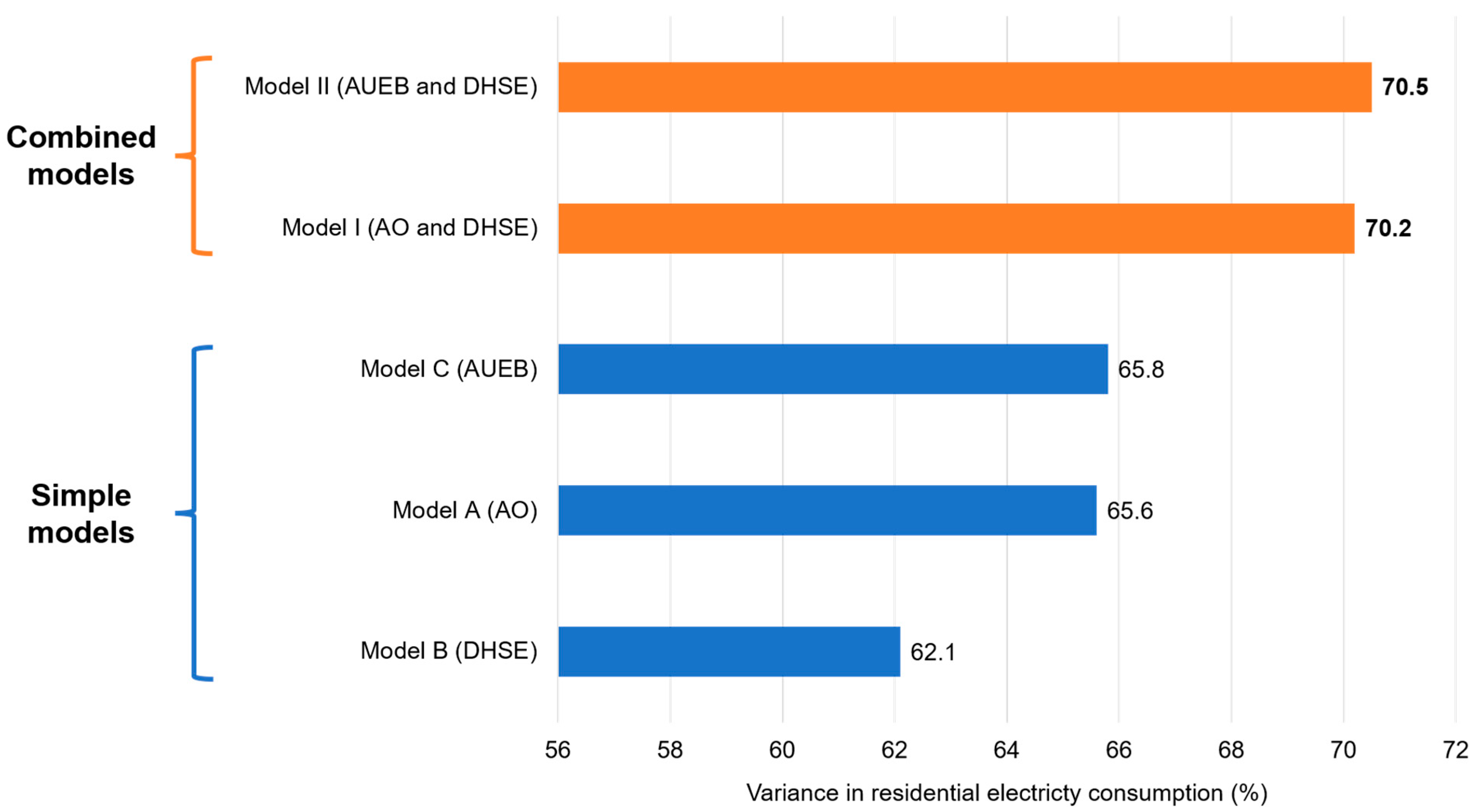
The statistical analyses were performed in this study to investigate the drivers of REC regarding DHSE characteristics, and the AO and AUEB factors. Three simple regression models were computed, after correlation analysis was performed, seeking to find the significantly correlated variables in regard to REC. The first model (Model A), constructed from the AO factors, explained 65.6% of the variance in the REC, with the most significant (p < 0.001) predictors of REC found to be the ownership of lighting, fridges and freezers and fans, followed by the ownership of air conditioners (p < 0.01), while the last group (p < 0.05) included the ownership of TV sets, microwaves and irons.

The second model, built with the DHSE characteristics, explained 62.1% of the variance in the REC. The most significant predictors (p < 0.001) for this model included the floor area, dwelling tenure type and household income, followed by the education level of the HRP and presence in the living room during the daytime (p < 0.01) and the overall presence in the bedroom (p < 0.05).

The last model, built using the AUEB factors, explained 65.8% of the variance in the REC. The use of lighting, TV sets, fridges, freezers, fans and air conditioners emerged as the most significant predictors (p < 0.001) of REC for this model, followed by the awareness of standby electricity consumption (SEC) and the use of games consoles (p < 0.05).

Finally, the significant factors from the three models were used to build two combined models (I and II) to investigate, separately, the effect of AO and AUEB factors on the REC when combined with the DHSE factors. On the one hand, the combined model I, which was built using the DHSE and AO factors, explained 70.8% of the variance in the REC, with significant predictors including household income, ownership of fridges and freezers (p < 0.001), followed by the dwelling tenure type and ownership of lighting, fans and air conditioners (p < 0.01), while the ownership of irons and the presence in rooms were found to be significant at the 5% level. On the other hand, the combined Model II, which was built using the DHES and AUEB factors, explained 70.5% of the variance in the REC. The most significant predictors in this model again included the household income and use of fridges and freezers, and also the use of TV sets (p < 0.001), while other significant predictors included the dwelling tenure type, use of lighting, use of air conditioners and the overall presence in the bedroom (p < 0.01).

Figure 4 summarises the variance in the REC explained by each model, while the significant factors are discussed below in comparison to the existing literature on determinants of REC and the policy implications and application of the research results.

5.1. DHSE Determinants of Residential Electricity Use

Three DHSE factors unanimously (found to be significant in all the models in which it was used as a predictor) emerged as significant predictors of residential electricity consumption (REC), namely household income, dwelling tenure type and overall presence in the bedroom (Table 5, Table 7, Table 8, Table A9, Table A10 and Table A11). The results demonstrate that households living in free (free rent households generally refers to occupiers that do not pay any fees for living in the dwelling, even if they are not the owner of the dwelling. Most of the time they are relatives or friends of the owner) and privately rented dwellings use up to 27% and 15% less electricity than those living in owner-occupied dwellings. These results are similar to those of Hamilton et al. [50], who found that owner-occupied homes use on average 25% more electricity than rented homes. Similarly, Wyatt [51] found that owner-occupied homes use on average 23% more electricity than housing association and council housing homes and 14% more than privately rented homes. Buying land and housing in urban areas in Burkina Faso is expensive, especially for recently built homes (after the 2000s). Therefore, most owner-occupied homes are owned by wealthy people, who can, therefore, also afford to purchase a large range of appliances and use them. Owner-occupied dwellings also tend to be larger than rented dwellings, and therefore consume more electricity, for the use of HVAC systems for example, where installed.

The results demonstrate that households with a monthly income of more than USD 1426 used 132%, 83% and 48% more electricity than incomes up to USD 168, USD 168–419 and USD 419–671, respectively. These findings are consistent with those of Yohanis et al. [23], Santamouris et al. [52] and Wyatt [51], who found that the highest-income households use 2.5, 1.9 and 1.6 times more electricity than the lowest-income households in Northern Ireland, the UK and Greece, respectively. This finding could be explained as the greater the household economic situation, the more the household can afford to purchase and use appliances.

The overall presence in the bedroom was also identified as a significant predictor of REC. A unit rise (hour) in the presence in the bedroom throughout the day results in an up to 3% increase in the annual REC. This finding is in line with that of Baker and Rylatt [53], who found that the weekly hours of presence in a dwelling positively affected the REC. Indeed, the presence of householders at home for a greater number of hours per week most likely implies the use of additional electricity for activities, such as homework, using a desktop or laptop, or the use of HVAC for comfort.

Some other factors were found to be significant but not unanimously (generally significant in the individual effect models (A–C), but not in the combined effect models (I and II)). Floor area was found to be significant only in Model B (individual effect of the DHSE factors), with a unit rise in floor area (m²) resulting in an increase in the REC of 0.2%. This complies with the findings by Sakah et al. [17], who found that an increase of 1 m² in the floor area increases the REC by 2.1%. Similarly, Zhou and Teng [33] reported an Increase in the REC of 0.6% for a 1% increase in the dwelling size.

Also, the education level of the HRP was also significant in model B. For example, homes with an HRP that completed university studies use 16% and 17% more electricity, respectively, than homes with an HRP that only completed secondary and primary school studies, and 22% more than those that never went to school. Similar results were reported by Zhou and Teng [33] and Leahy and Lyons [25] for Chinese and Irish families.

Finally, presence in the living room was significant only in Models B and I, with a unit rise in the daytime presence in the living room resulting in an increase in the REC of up to 2.5%.

5.2. AO Determinants of Residential Electricity Use

Significant predictors of REC concerning the AO factors include the ownership of common (appliances that demonstrated an ownership rate of at least 70%) appliances, like lighting fixtures, fans and fridges, but also less commonly owned but heavy appliances like irons, freezers and air conditioners (Table 4, Table 7 and Table A10). An additional unit of lighting fixtures, fans and fridges in the appliance stock increases the annual REC by 2%, 6% and 22%, respectively. A positive and significant effect on the REC was also previously reported by Sakah et al. [17] regarding the ownership of such appliances. They found that the REC increases, respectively, by 87 kWh (3%), 226 kWh (7%) and 649 kWh (20%) with a unit rise in the lighting fixtures, fridges and fans. The significant and positive effect of fridges on the REC has also been widely reported in other residential electricity use studies [26,32,33], with for example, Zhou and Teng [33], reporting that households with a fridge use 22% more electricity than those without.

The findings also show that a unit rise in irons, air conditioners and freezers in the appliance stock results in an increase in the REC of 12%, 10% and 29%. Here, freezers and air conditioners were also found to be significant predictors of REC in the literature [31,32]. For example, Sakah et al. [17] reported an increase in the annual REC by 886 kWh (27%) and 1990 kWh (61%), respectively, per unit increase in the ownership of freezers and ACs.

Finally, appliances like television sets and microwaves were significant in the model built using the AO factors only (Model A), but not in the combined effect model using the AO and DHSE factors. A unit rise in the ownership of TV sets was associated with an increase in the REC of 4%, while that of a microwave was associated with an increase in the REC of 15%. Televisions have been widely acknowledged as significant predictors, positively affecting electricity use [17,31,32,53]. To date microwaves have been investigated less, with existing studies reporting no effect on REC [25].

5.3. AUEB Determinants of Residential Electricity Use

Significant predictors of REC regarding the AUEB factors include the use of common appliances like lighting fixtures, TV sets and fridges, but also less common appliances like freezers and air conditioners (Table 6, Table 8 and Table A11). The use of lighting, TV sets and fridges has a positive effect on REC. A unit rise (1 h) in the duration of the use of lighting, TV sets and fridges increases the annual REC by 0.4%, 1% and 1.4%. Even though little research was found in the literature on the effect of appliance use on REC, such findings are similar to those of Bedir et al. [29], who explained 37% and 58%, respectively, of the variance in REC with models built on appliance use and presence factors, and appliance use and DHSE factors. TV use was also reported as having a significant and positive effect on REC within US households by Sanquist [54].

The findings also show a significant and positive effect of air conditioners and freezers on REC, with an increase in the annual REC of 5% and 1%, respectively, associated with a unit rise (1 h) in their daily use. Contrary to such findings, Bedir et al. [29] reported that cooking appliances in which freezers were classified did not affect REC, whilst extra ventilation appliances, including air conditioners, were not found to be correlated with REC in their study.

Other variables, including the use of fans and games consoles and the awareness of standby electricity consumption, were significant in the model built using only the AUEB factors, but not in the combined model using the AUEB and DHSE factors. A unit rise in the use of fans (1 h) is associated with an increase in annual REC by 1.1%. On the other hand, an increase in the use of games consoles (perhaps) unexpectantly resulted in a decrease in the REC by 5%. This finding warrants further investigation. It may be hypothesised that the increased use games consoles results in households avoiding other more electricity-consuming activities.

Also, it was demonstrated that households that are aware of standby electricity consumption use 9% more electricity. This finding may also be unanticipated as understanding that appliances consume electricity in standby mode would presumably lead to households’ switching off their appliances rather than using standby. However, this finding compares well to the authors’ previous research [20], which established that households headed by an HRP with a higher level of education are more informed of standby consumption, but equally, a higher level of education is associated with a higher economic level and, therefore, higher appliance ownership and use, and increased REC.

Finally, contrary to the opinion of Zhou and Teng [33], and the findings by Bedir et al. [29], who demonstrated that appliance use affects REC more than appliance ownership, the current study found very little difference between the effects of the two categories of factors on REC. Either individually (65.6 and 65.8% of the variance in the REC) or combined with the DHSE factors (70.2 and 70.5% of the variance in the REC), the AO and AUEB factors demonstrated almost the same effect on the REC. This may be explained by the fact that most of the appliances found to be significant predictors of REC had the highest ownership and use in the households’ appliance stock. This includes mainly lighting fixtures, fridges, TV sets, fans and ACs.

5.4. Policy Implications and Applications for Research

The current study used data collected from a survey of 387 households in the city of Ouagadougou to analyse the determinants of REC in urban households in Burkina Faso. The analysed determinants included DHSE characteristics, AO and AUEB factors.

Household income and tenure type were identified as unambiguous predictors of REC, affecting it positively. This suggests that the economic level is the main DHSE factor to consider for REC prediction and policy implementation. As a critical objective of countries in the Global South in the coming years, economic development can be expected to lead to an increase in REC. Future policies should, therefore, consider this economic dimension. For example, policy incentives could be used to encourage the purchase of more efficient appliances, or demand-side management (DSM) strategies like load curtailment programmes could also be used.

This study demonstrated similar findings to other studies on Global South countries concerning appliance ownership and use. Indeed, the ownership and use of a range of common domestic appliances were identified as significant predictors of REC, also affecting it positively. Such appliances, including lighting fixtures, TV sets, fans, fridges, freezers and ACs, which should serve as primary targets for energy efficiency/conservation policies and DSM strategies.

Unusually, households in this study that were aware of energy conservation used 9% more electricity. Significant effort is, therefore, needed to ensure energy efficiency information and campaigns are translated into expected demand reduction in future.

The results from this study should be of great interest to a range of stakeholders in the electricity sector, not only Burkina Faso, but also other countries that share common characteristics. Indeed, it should significantly help in estimating current and future residential electricity consumption due to changes in the socio-economic and dwelling characteristics of households, and the patterns of appliance ownership and use. In this sense, the findings should not only interest decisionmakers and policymakers in designing and implementing more tailored energy efficiency/conservation policies in the residential sector, but also (electricity) utility services for future planning concerning the demand on the electrical network in the country, as well as the implementation of DSM strategies, such as demand response programmes. It could also be of key importance to energy modellers and developers of integrated renewable energy systems for buildings as information on electricity use and its influencing factors were revealed. Also, the information could interest householders wishing to review their behaviour or patterns of use in order to reduce their electricity bills.

5.5. Limitations of the Study and Future Research

Aiming to reduce the paucity of information on REC in Burkina Faso and the Global South, this study provides several insights on the influence of household characteristics and behaviours on REC. However, the current findings are limited by some restrictions explained below.

First, the sample size is limited. In the current study, the sample size was designed due to constraints like the costs associated with data collection. Larger sample sizes are needed for future research to validate the results obtained in this study and to extend the research on REC to other areas in Burkina Faso.

Self-reported data provided by households during interviews may have caused bias. Some households may feel observed even after agreeing to participate, leading to differences between their actual characteristics and behaviours and those reported. A solution for future studies is in situ measurements of occupancy and usage patterns of appliances, which will also help conduct research on aspects like occupants’ behaviours.

Electricity bills were used for estimating the electricity consumption of households. However, future research could use direct measurements of electricity consumption using sensors. This would provide higher-resolution data, opening up more opportunities for analyses of domestic REC, such as the effects of appliance usage patterns on real-time REC.

Finally, other external factors concerning dwellings, including the effect of the environment, electricity price, policies and dwelling location, which were not part of this study’s scope could be investigated.

Although such limitations can be suggested, the current study’s findings stand, as the results can serve as a basis for forthcoming studies in Burkina Faso and other countries with similar characteristics. Also, it provides useful insights for energy planners, designers and policymakers as some information, like the prediction of REC with DHSE and appliance factors, is a valuable asset for all electricity sector actors.

6. Conclusions

This study used the data collected from 387 households in the city of Ouagadougou to provide insights into the effects of DHSE, AO and AUEB factors on urban REC in Burkina Faso. Three simple models (A to C) were built first to investigate the individual effects of the DHSE, AO and AUEB factors on REC. With the identified significant predictors of each model, two other models were built to assess the combined effects of the DHSE and AO factors (Model I), and the DHSE and AUEB factors (Model II), on REC. The key findings of the study were:

• The DHSE factors individually explained 62.1% of the variance in the REC and 70.2% and 70.5%, respectively, when combined with the AO and AUEB factors. The unambiguously significant DHSE predictors of REC were household income and dwelling tenure type, with the highest-income households using up to 1.32 times more electricity than the lowest-income households. Owner-occupied households use up to 34% more electricity than rented dwelling households.
• The AO factors individually explained 65.6% of the variance in the REC and 70.2% when combined with the DHSE factors. The unambiguously significant AO predictors of REC were the ownership of lighting fixtures, fans, fridges, irons, freezers and air conditioners. The ownerships of TV sets and microwaves were significant in the model built for the AO factors only.
• Alone, the AUEB factors explained 65.8% of the variance in the REC and 70.5% when combined with the DHSE factors. The unambiguously significant predictors of REC include the use of lighting fixtures, TV sets, fridges, freezers and air conditioners. The use of fans and games consoles and the awareness of standby electricity consumption were significant factors in the model using the AUEB factors only.
• No differences between the effects of appliance ownership and appliance use on REC were identified, contrary to previous studies. Individually or when combined with the DHSE factors, the AO and AUEB factors explained almost the same share of variance in the REC (up to 70.2% and 70.5%).

References

1. Mutumbi, U.; Thondhlana, G.; Ruwanza, S. Reported behavioural patterns of electricity use among low-income households in Makhanda, South Africa. Sustainability 2021, 13, 7271. [Google Scholar] [CrossRef]
2. Wassie, Y.T.; Adaramola, M.S. Socio-economic and environmental impacts of rural electrification with Solar Photovoltaic systems: Evidence from southern Ethiopia. Energy Sustain. Dev. 2021, 60, 52–66. [Google Scholar] [CrossRef]
3. UEMOA. Atlas de L’énergie dans L’espace UEMOA. 2020. Available online: https://www.ifdd.francophonie.org/publications/atlas-de-lenergie-dans-lespace-uemoa/ (accessed on 1 October 2021).
4. Wethe, J. Systèmes Énergétiques: Vulnérabilité—Adaptation—Résilience (VAR): Burkina Faso; HELIO International: Ho Chi Minh City, Vietnam, 2009; pp. 1–48. Available online: https://www.academia.edu/3567464/Burkina_Faso (accessed on 10 April 2022).
5. Jones, R.V.; Lomas, K.J. Determinants of high electrical energy demand in UK homes: Appliance ownership and use. Energy Build. 2016, 117, 71–82. [Google Scholar] [CrossRef]
6. Cabeza, L.F.; Ürge-Vorsatz, D.; Palacios, A.; Ürge, D.; Serrano, S.; Barreneche, C. Trends in penetration and ownership of household appliances. Renew. Sustain. Energy Rev. 2018, 82, 4044–4059. [Google Scholar] [CrossRef]
7. Le, V.T.; Pitts, A. A survey on electrical appliance use and energy consumption in Vietnamese households: Case study of Tuy Hoa city. Energy Build. 2019, 197, 229–241. [Google Scholar] [CrossRef]
8. Yoshida, A.; Manomivibool, P.; Tasaki, T.; Unroj, P. Qualitative study on electricity consumption of urban and rural households in Chiang Rai, Thailand, with a focus on ownership and use of air conditioners. Sustainability 2020, 12, 5796. [Google Scholar] [CrossRef]
9. Genjo, K.; Tanabe, S.; Matsumoto, S.; Hasegawa, K.; Yoshino, H. Relationship between possession of electric appliances and electricity for lighting and others in Japanese households. Energy Build. 2005, 37, 259–272. [Google Scholar] [CrossRef]
10. Singh, J.; Mantha, S.S.; Phalle, V.M. Analysis of technical and economic electricity saving potential in the urban Indian households. Sustain. Cities Soc. 2018, 43, 432–442. [Google Scholar] [CrossRef]
11. Kim, M.; Jung, S.; Kang, J.W. Artificial neural network-based residential energy consumption prediction models considering residential building information and user features in South Korea. Sustainability 2020, 12, 109. [Google Scholar] [CrossRef]
12. Williams, S.P.; Thondhlana, G.; Kua, H.W. Electricity use behaviour in a high-income neighbourhood in Johannesburg, South Africa. Sustainability 2020, 12, 4571. [Google Scholar] [CrossRef]
13. Bohlmann, J.A.; Inglesi-Lotz, R. Examining the determinants of electricity demand by South African households per income level. Energy Policy 2021, 148, 111901. [Google Scholar] [CrossRef]
14. Ye, Y.; Koch, S.F.; Zhang, J. Determinants of household electricity consumption in South Africa. Energy Econ. 2018, 75, 120–133. [Google Scholar] [CrossRef]
15. Diawuo, F.A.; Sakah, M.; Pina, A.; Baptista, P.C.; Silva, C.A. Disaggregation and characterization of residential electricity use: Analysis for Ghana. Sustain. Cities Soc. 2019, 48, 101586. [Google Scholar] [CrossRef]
16. Diawuo, F.A.; Sakah, M.; de la Rue du Can, S.; Baptista, P.C.; Silva, C.A. Assessment of multiple-based demand response actions for peak residential electricity reduction in Ghana. Sustain. Cities Soc. 2020, 59, 102235. [Google Scholar] [CrossRef]
17. Sakah, M.; de la Rue du Can, S.; Diawuo, F.A.; Sedzro, M.D.; Kuhn, C. A study of appliance ownership and electricity consumption determinants in urban Ghanaian households. Sustain. Cities Soc. 2019, 44, 559–581. [Google Scholar] [CrossRef]
18. Akrofi, M.M.; Okitasari, M. Beyond costs: How urban form could limit the uptake of residential solar PV systems in low-income neighborhoods in Ghana. Energy Sustain. Dev. 2023, 74, 20–33. [Google Scholar] [CrossRef]
19. Danlami, A.H. Determinants of Household Electricity Consumption in Bauchi State, Nigeria. Hyperion Econ. J. 2017, 5, 16–28. [Google Scholar]
20. Tete, K.H.S.; Soro, Y.M.; Sidibé, S.S.; Jones, R. V Urban domestic electricity consumption in relation to households’ lifestyles and energy behaviours in Burkina Faso: Findings from a large-scale, city-wide household survey. Energy Build. 2023, 285, 18. [Google Scholar] [CrossRef]
21. Mcloughlin, F. Characterising Domestic Electricity Demand for Customer Load Profile Segmentation. Ph.D. Thesis, Technological University Dublin, Dublin, Ireland, 2013. [Google Scholar] [CrossRef]
22. O’Doherty, J.; Lyons, S.; Tol, R.S.J. Energy-using appliances and energy-saving features: Determinants of ownership in Ireland. Appl. Energy 2008, 85, 650–662. [Google Scholar] [CrossRef]
23. Yohanis, Y.G.; Mondol, J.D.; Wright, A.; Norton, B. Real-life energy use in the UK: How occupancy and dwelling characteristics affect domestic electricity use. Energy Build. 2008, 40, 1053–1059. [Google Scholar] [CrossRef]
24. Jones, R.V.; Fuertes, A.; Lomas, K.J. The socio-economic, dwelling and appliance related factors affecting electricity consumption in domestic buildings. Renew. Sustain. Energy Rev. 2015, 43, 901–917. [Google Scholar] [CrossRef]
25. Leahy, E.; Lyons Sean, S. Energy use and appliance ownership in Ireland. Energy Policy 2010, 38, 4265–4279. [Google Scholar] [CrossRef]
26. Bartiaux, F.; Gram-hanssen, K. Socio-Political Factors Influencing Household Electricity Consumption: A Comparison between Denmark and Belgium; ECEEE Summer Study; ECEEE: Stockholm, Sweden, 2005; pp. 1313–1325. [Google Scholar]
27. Gram-Hanssen, K.; Kofod, C.; Petersen, K.N. Different Everyday Lives—Different Patterns of Electricity Use. In Proceedings of the 2004 ACEEE Summer Study on Energy Efficiency in Buildings, Pacific Grove, CA, USA, 22–27 August 2004; pp. 1–13. [Google Scholar]
28. Bartusch, C.; Odlare, M.; Wallin, F.; Wester, L. Exploring variance in residential electricity consumption: Household features and building properties. Appl. Energy 2012, 92, 637–643. [Google Scholar] [CrossRef]
29. Bedir, M.; Hasselaar, E.; Itard, L. Determinants of electricity consumption in Dutch dwellings. Energy Build. 2013, 58, 194–207. [Google Scholar] [CrossRef]
30. Esmaeilimoakher, P.; Urmee, T.; Pryor, T.; Baverstock, G. Identifying the determinants of residential electricity consumption for social housing in Perth, Western Australia. Energy Build. 2016, 133, 403–413. [Google Scholar] [CrossRef]
31. McLoughlin, F.; Duffy, A.; Conlon, M. Characterising domestic electricity consumption patterns by dwelling and occupant socio-economic variables: An Irish case study. Energy Build. 2012, 48, 240–248. [Google Scholar] [CrossRef]
32. Kavousian, A.; Rajagopal, R.; Fischer, M. Determinants of residential electricity consumption: Using smart meter data to examine the effect of climate, building characteristics, appliance stock, and occupants’ behavior. Energy 2013, 55, 184–194. [Google Scholar] [CrossRef]
33. Zhou, S.; Teng, F. Estimation of urban residential electricity demand in China using household survey data. Energy Policy 2013, 61, 394–402. [Google Scholar] [CrossRef]
34. Fan, H.; MacGill, I.F.; Sproul, A.B. Statistical analysis of drivers of residential peak electricity demand. Energy Build. 2017, 141, 205–217. [Google Scholar] [CrossRef]
35. MEMC/BF. Tableau de Bord 2020 du Ministère de L’energie, des Mines et des Carrières. 2020. Available online: http://cns.bf/IMG/pdf/tableau_de_bord_2020_memc.pdf (accessed on 12 October 2022).
36. INSD-BF. Cinquième Recensement Général de la Population et de L’habitation du Burkina Faso (5e RGPH): Synthèse des Résultats Définitifs. 2022. Available online: https://www.insd.bf/fr/file-download/download/public/2071 (accessed on 6 February 2023).
37. MEF/BF. Monographie de la Commune Urbaine de Ouagadougou. 2009. Available online: https://ireda.ceped.org/inventaire/ressources/bfa-2006-rec-o2_commune_urbaine_ouagadougou.pdf (accessed on 12 August 2022).
38. Kabore, B.; Kam, S.; Ouedraogo, G.W.P.; Bathiebo, D.J. Etude de l’evolution climatique au Burkina Faso de 1983 à 2012: Cas des villes de Bobo Dioulasso, Ouagadougou et Dori. Arab. J. Earth Sci. 2017, 4, 50–59. [Google Scholar]
39. Massieke Soma, A.A.R.; Tapsoba, F.W.; Kabore, D.; Seogo, I.; Tankoano, A.; Dicko, M.H.; Toguyeni, A.; Sawadogo-Lingani, H. Etude sur la capacité de production, du circuit de commercialisation et de la consommation du zoom-koom vendu dans la ville de Ouagadougou au Burkina Faso. Int. J. Biol. Chem. Sci. 2018, 11, 2294. [Google Scholar] [CrossRef]
40. Cochran, W.G. Sampling Techniques. 1977. Available online: https://fsapps.nwcg.gov/gtac/CourseDownloads/IP/Cambodia/FlashDrive/Supporting_Documentation/Cochran_1977_Sampling%20Techniques.pdf (accessed on 14 January 2021).
41. Uakarn, C. Sample size estimation using Yamane and Cochran and Krejcie and Morgan and Green formulas and Cohen statistical power analysis by G*power and comparisons. Apheit Int. J. 2021, 10, 76–88. [Google Scholar]
42. Adam, A.M. Sample Size Determination in Survey Research. J. Sci. Res. Rep. 2020, 26, 90–97. [Google Scholar] [CrossRef]
43. Sukarno, I.; Matsumoto, H.; Susanti, L. Household lifestyle effect on residential electrical energy consumption in Indonesia: On-site measurement methods. Urban Clim. 2017, 20, 20–32. [Google Scholar] [CrossRef]
44. Mohammad, A.; Shrestha, P.; Kumar, S. Urban residential energy use in Kandahar, Afghanistan. Cities 2013, 32, 135–142. [Google Scholar] [CrossRef]
45. Hong, T.; Yan, D.; D’Oca, S.; Chen, C.-f. Ten questions concerning occupant behavior in buildings: The big picture. Build. Environ. 2017, 114, 518–530. [Google Scholar] [CrossRef]
46. Carpino, C.; Mora, D.; De Simone, M. On the use of questionnaire in residential buildings. A review of collected data, methodologies and objectives. Energy Build. 2019, 186, 297–318. [Google Scholar] [CrossRef]
47. Aglina, M.K.; Agbejule, A.; Nyamuame, G.Y. Policy framework on energy access and key development indicators: ECOWAS interventions and the case of Ghana. Energy Policy 2016, 97, 332–342. [Google Scholar] [CrossRef]
48. Field, A. Discovering Statistics Using IBM SPSS Statistics; Sage Publications, Inc.: Thousand Oaks, CA, USA, 2018. [Google Scholar]
49. Cook, R.D.; Weisberg, S. Residuals and Influence in Regression. 1982, p. 230. Available online: http://conservancy.umn.edu/handle/11299/37076 (accessed on 12 December 2022).
50. Hamilton, I.G.; Steadman, P.J.; Bruhns, H.; Summerfield, A.J.; Lowe, R. Energy efficiency in the British housing stock: Energy demand and the Homes Energy Efficiency Database. Energy Policy 2013, 60, 462–480. [Google Scholar] [CrossRef]
51. Wyatt, P. A dwelling-level investigation into the physical and socio-economic drivers of domestic energy consumption in England. Energy Policy 2013, 60, 540–549. [Google Scholar] [CrossRef]
52. Santamouris, M.; Kapsis, K.; Korres, D.; Livada, I.; Pavlou, C.; Assimakopoulos, M.N. On the relation between the energy and social characteristics of the residential sector. Energy Build. 2007, 39, 893–905. [Google Scholar] [CrossRef]
53. Baker, K.J.; Rylatt, R.M. Improving the prediction of UK domestic energy-demand using annual consumption-data. Appl. Energy 2008, 85, 475–482. [Google Scholar] [CrossRef]
54. Sanquist, T.F.; Orr, H.; Shui, B.; Bittner, A.C. Lifestyle factors in U.S. residential electricity consumption. Energy Policy 2012, 42, 354–364. [Google Scholar] [CrossRef]
Figure 1. Map of Ouagadougou and its 12 districts (adapted from [39]).
Buildings 14 00683 g001
Figure 2. Background of the survey.
Buildings 14 00683 g002
Figure 3. Study framework: data processing methodology.
Buildings 14 00683 g003
Figure 4. Variance in REC explained by the variables in the studied models.
Buildings 14 00683 g004