Theoretical Model for the Stress–Strain Curve of CNT-Reinforced Concrete under Uniaxial Compression

Abstract

The incorporation of carbon nanotubes (CNTs) can enhance the mechanical properties of concrete. The stress–strain curves of CNT-reinforced concrete under uniaxial compression are investigated through an experimental program with different CNT and steel fiber proportions considered. The test results demonstrate that CNTs can increase both peak stress and peak strain, and steel fibers can further enhance the effect of CNTs. Additionally, steel fibers can effectively enhance both the strength and ductility. Theoretical models for the peak strain, initial elastic modulus, toughness index and relative absorbed energy are established. A theoretical model for the uniaxial compressive constitutive relationship of CNT-reinforced concrete considering CNT and steel fiber content is developed. Finite element (FE) modelling is developed to simulate the axial compression behavior of CNT-reinforced concrete.

1. Introduction

The brittleness of ordinary concrete materials has long been a subject of concern. Studies have revealed that reinforcing fibers, such as steel, glass, and polymer fibers, can effectively mitigate crack development in concrete and enhance the mechanical properties and durability of concrete [1,2,3,4]. However, the application of conventional fibers alone is insufficient to prevent the emergence and propagation of nanoscale cracks, which can lead to a decline in concrete strength during the later stages due to crack development [5]. The large specific surface area of nanomaterials enables them to fully interact with the cement matrix, and their minute size enables them to fill the nanoscale pores within the concrete, facilitating the formation of a denser microstructure and also the control of matrix cracks at the nanoscale level [6]. CNTs are typically envisioned as rolled single sheets of graphene and are classified as single-wall carbon nanotubes (SWCNTs) or multi-wall carbon nanotubes (MWCNTs) according to the number of graphene layers, as illustrated in Figure 1 [7]. The price of SWCNTs is USD 37,500 to USD 160,000 per kg and that for MWCNTs is USD 0600 to USD 15,000 per kg [8]. For other carbon-based materials, carbon nanofibers (CNFs) are quasi-one-dimensional carbon materials with diameters larger than CNTs, and graphene nanoplatelets (GNPs) consist of several graphene layers with an overall thickness in the nanometer scale. The tensile strength of CNFs and GNPs is 2.7–7 GPa and 10–25 GPa, respectively. Among these carbon-based materials, CNTs have the highest tensile strength of 10–500 GPa [9]. CNTs and CNFs are considered to be the most effective nanomaterials for improving the mechanical properties of concrete, exhibiting properties such as self-sensing [10]. Researchers have also reported that compared with other carbon-based materials like GNPs, which can also be used as nanoreinforcements in cement-based composites, CNTs can enhance the flexural strength of concrete more effectively due to their high aspect ratio and cylindrical structure, which enable CNTs to bridge nano-cracks more easily [11].

As a novel nanomaterial, CNTs exhibit exceptional mechanical properties and have the characteristics of a light weight and small sizes [12,13,14]. CNTs can improve the mechanical properties of concrete, such as its tensile strength, compressive strength, flexural strength and impact toughness, due to the bridging effect. CNTs can also fill the internal pores, reduce porosity and thus enhance durability. Additionally, CNTs can decrease the resistivity of materials effectively and work as conductive fillers in self-sensing concrete [5,15].

Jiang et al. investigated the strengthening effect of CNTs in cement-based material and compared it with three other nanomaterials, namely nano-SiO₂ (NS), nano-TiO₂ (NT), and CNFs [16]. The results show that the incorporation of 0.1% NS, 0.5% NT, 0.1% CNTs, and 0.5% CNFs increased the compressive strength of the concrete by 12.5%, 20.8%, 16.8%, and 21.4%, respectively, compared to concrete without nanomaterials. Additionally, CNTs and CNFs were found to enhance electrical conductivity in the composites. The impact of CNT content on the mechanical properties of cement-based composites was investigated [16,17,18,19,20,21]. It was confirmed that CNTs can enhance the mechanical properties of cement-based materials. However, excessive CNT content can diminish this improvement effect. Gillani et al. obtained the crack mouth opening displacement–bending stress curves of concrete with MWCNTs from experimental study [19]. Wang et al. examined the bending toughness of cement-based composites containing MWCNTs and observed a more uniform pore size distribution and reduced porosity after adding MWCNTs [21]. The large surface area and length-to-diameter ratio of CNTs may result in strong van der Waals forces between individual nanotubes, leading to agglomeration and clustering, and this may weaken their reinforcing effect [22]. Surfactants and ultrasonic treatment are commonly employed to disperse CNTs. Due to the presence of van der Waals forces, ultrasonic treatment can temporarily disperse CNTs [23], while surfactants prevent the reaggregation of CNTs [24]. Graphene oxide (GO) is an excellent hydrophilic material with excellent dispersion properties in aqueous solutions because of its oxygen-containing functional groups such as carbonyl, hydroxyl and carboxyl [25]. Researchers have reported that CNTs exhibit optimal dispersion in the GO solution due to the supramolecular interactions between CNTs and GO, and the electronegativity of the GO solution, which is caused by the ionization of the phenol hydroxyl and carboxyl groups [25,26]. Thus, GO was selected as the dispersant of CNTs in this study. Parveen et al. summarized the effects of different dispersion techniques on the microstructure and mechanical properties of cement-based materials enhanced by various types of CNT [27]. The research on the effect of CNTs on the mechanical properties of concrete is summarized in

Table 1. Relevant research on mechanical properties of CNT-reinforced concrete.

Literature	Amount of CNT (% of Cement)	Dispersion Technique	Properties	Increase (%)
Jiang et al. [16]	0.1, 0.5, 1.0	US 1	CS 2	16.8, 10.0, −3.5
Kumar et al. [17]	0.5, 0.75, 1.0	US	CS	13.7, 1.5, −25.7
			STS 3	16.7, 4.4, −21.8
Chaipanich et al. [18]	0.5, 1.0	US	CS	6.4, 4.1
			FS 4	2.9, 2.3
Gillani et al. [19]	0.05, 0.1	ST 5 and US	CS	19.1, 24.7
			STS	26.0, 18.0
Xu et al. [20]	0.025, 0.05, 0.1	ST and US	CS	6.3, 12.7, 14.6
	0.025, 0.05, 0.1, 0.2		STS	7.5, 15.0, 30.0, 40.0
Wang et al. [21]	0.05, 0.08, 0.10, 0.12, 0.15	ST and US	FTI 6	31.0, 57.5, 47.1, 31.6, 10.3
Nochaiya et al. [28]	1.0	US	TP 7	16.0
Li et al. [29]	0.5	HMF 8	CS	18.9
			FS	25.1
			TP	39.2
Musso et al. [30]	0.5	AS 9 and US	CS	10.6
Al-Rub et al. [31]	0.2	SP 10 and US	FS	269.0
			D 11	81.0
Konsta-Gdoutos et al. [32]	0.08	ST and US	YM 12	45.0
			FS	25.0
Luo et al. [33]	0.2	MS 13, ST and US	CS	29.5
			FS	35.4
Collins et al. [34]	0.5	MS, PCA 14 and US	CS	25.0
Cwirzen et al. [35]	0.045	CF 15, PAP 16 and US	CS	50.0

¹ US: ultrasonication; ² CS: compressive strength; ³ STS: splitting-tensile strength; ⁴ FS: flexural strength; ⁵ ST: surfactant; ⁶ FTI: flexural toughness index; ⁷ TP: total porosity; ⁸ HMF: HNO3/H2SO4 mixture functionalization; ⁹ AS: acetone solvent; ¹⁰ SP: superplasticizer; ¹¹ D: ductility; ¹² YM: Young’s modulus; ¹³ MS: magnetic stirring; ¹⁴ PCA: poly carboxylate admixture; ¹⁵ CF: carboxylic functionalization; ¹⁶ PAP: polyacrylic acid polymer.

[16,17,18,19,20,21,28,29,30,31,32,33,34,35].

Studies on the stress–strain behavior of CNT-reinforced concrete under uniaxial compression are limited, and no studies have been conducted on the theoretical model for the constitutive relationship of CNT-reinforced concrete to the authors’ knowledge to date. The compressive performance of CNT-reinforced concrete is investigated in this study. The influence of the CNT and steel fiber content on uniaxial compressive stress–strain curves is analyzed through an experimental program. The theoretical models for the peak strain, initial elastic modulus, toughness index, relative absorbed energy and also the stress–strain curves are developed, and finite element modeling is performed.

2. Experiment

2.1. Experimental Program

2.1.1. Materials

In this study, the materials could be divided into three parts. The first part consisted of cement, fine sand, silica fume, quartz powder, a water-reducing agent and an accelerator, constituting the cement-based component of CNT-reinforced concrete. The second part included CNTs and GO. The third part consisted of steel fibers.

P·O 42.5 cement was used, and the average particle size of cement was 17 μm. Natural sand with an average particle size of 487 μm was used. Silica fume with a bulk density of 350 kg/m³, an average particle size of 0.15 μm and a specific surface area of 21.658 m²/g was used. A quartz powder with a density of 2.3 g/cm³ and an average particle size of 44 μm was selected. A polycarboxylate-based superplasticizer with a solid content of 41% and a water reducing rate of 30% was used. A calcium chloride-based accelerator produced by Sakrete of North America LLC in the USA was used. NC7000^TM CNTs produced by Nanocyl SA in Belgium were used, and their physical properties are listed in

Table 2. Physical properties of CNTs.

Average Diameter of Outer Layer (nm)	Average Diameter of Inner Layer (nm)	Average Length (μm)	Surface Area (m2/g)	Loose Bulk Density (g/cm3)	Tapped Bulk Density (g/cm3)
>50	5~15	15	250~300	0.18	2.1

. The GO solution produced by Graphenea SA in Spain was used as a dispersant for CNTs, and its properties are provided in

Table 3. Physical and chemical properties of GO.

Particle Size (μm)	Solvent	Concentration (mg/mL)	pH	Proportion of Single-Layer GO Sheets (%)	Diameter of Single-Layer GO (μm)	Thickness (nm)
<10 μm	water	4	2.2~2.5	>95	0.5~5	0.8~12

. The physical and mechanical properties of the steel fibers used are listed in

Table 4. Physical and mechanical properties of steel fibers.

Length (mm)	Diameter (mm)	Length/ Diameter	Tensile Strength (MPa)	Number of Fibers (/kg)
13	0.22	60	2850	224,862

.

2.1.2. Mix Proportions

In this study, the mass fractions of CNTs were 0, 0.08%, and 0.5%. The volume fraction of steel fibers ranged from 0 to 2%. A total of 36 specimens were prepared, with 6 specimens for each mix proportion, and 3 specimens were tested at the ages of 7 days and 28 days, respectively, as summarized in

Table 5. Mix proportions.

Group	Cement	Silica Fume	Fine Sand	Quartz Powder	Water	Superplasticizer	Accelerator	CNT	GO	Steel Fiber *
C0S0	100	32.5	145	30	24	4.3	4.2	0	0	0
C0S2	100	32.5	145	30	24	4.3	4.2	0	0	2
C0.08S0	100	32.5	145	30	24	4.3	4.2	0.08	0.04	0
C0.08S2	100	32.5	145	30	24	4.3	4.2	0.08	0.04	2
C0.5S0	100	32.5	145	30	24	4.3	4.2	0.5	0.04	0
C0.5S2	100	32.5	145	30	24	4.3	4.2	0.5	0.04	2

* The steel fiber content is the volume fraction of the specimen, while contents of the other components are expressed as the weight ratio.

. In the group number, “C” and the number after it represent CNTs and their corresponding mass fraction (%), while “S” denotes steel fibers along with their volume fraction (%). For instance, “C0.08S2” refers to a mixture containing CNTs at a mass fraction of 0.08% and steel fibers at a volume fraction of 2%.

2.1.3. Specimen Fabrication

According to ASTM C39/C39M-17 [36], cylindrical specimens of Φ50 mm × 100 mm were fabricated. Prior to the mixing process, the dispersion of CNTs in the GO solution was conducted. The mixture of CNTs and the GO solution was stirred for 10 min, followed by ultrasonic treatment in a water bath at 25 ± 5 °C for 60 min. Then, the suspension was left to stand for 2 h, and it could be used if no precipitate was found. According to Qiu et al.’s study, CNTs can be well dispersed with a GO solution and ultrasonication for an hour [26].

Portland cement, fine sand, silica fume, and quartz powder were mixed for 2 min. The accelerator and half of the superplasticizer and CNT solution were slowly added within 30 s, and then stirred for 1 min. The remaining superplasticizer and CNT solution were then added and stirred for 15 min. Finally, the steel fibers were gradually introduced within 30 s followed by stirring for an additional 1 min. In accordance with ASTM C31/C31M-03 [37], half of the mixture was added into the mold and compacted and vibrated. Then, the remaining half was added and compacted and vibrated. According to ASTM C192/C192M-16a [38], the standard curing method was employed. Specimens were kept in the lab at 23 ± 2 °C for 24 h. After demolding, specimens were kept in the curing room with a temperature of 23 ± 2 °C and humidity above 90% until the tests.

2.1.4. Test Procedure

The MTS815.02 electro-hydraulic servo test system was employed. Following the calibration of axial load, the initial loading speed was 0.04 mm/min, and was reduced to 0.02 mm/min as the curve reached the gentle stage. The load was measured by the pressure sensor and deformation was measured using an Epsilon extensometer. All of the data were recorded. The test setup is shown in Figure 2.

2.2. Results and Discussion

2.2.1. Failure Modes

The influence of CNT content on the failure modes was investigated. As shown in Figure 3a–c for 7-day specimens without steel fibers, all specimens exhibited brittle failure, and no significant difference was observed in the failure modes as CNT content varied. Upon reaching the maximum stress, vertical cracks emerged abruptly and small fragments detached from the specimen surface, leading to all-through cracks and failure. CNT content had little influence on the failure process. As internal cracks propagated, CNTs could not mitigate millimeter-scale cracks, which resulted in brittle fracture.

Comparing Figure 3c and Figure 3d, the incorporation of steel fibers changed the failure mode from brittle failure to ductile failure. Unlike specimens without steel fibers, those containing 2% steel fibers exhibited the initial formation of small cracks at ultimate stress and still maintained certain load-bearing capacity. Cracks propagated gradually, and eventually all-through cracks formed. The presence of steel fibers at the crack interface played a crucial role in impeding crack growth.

Regarding the failure mode of specimens at different ages, no significant difference was observed.

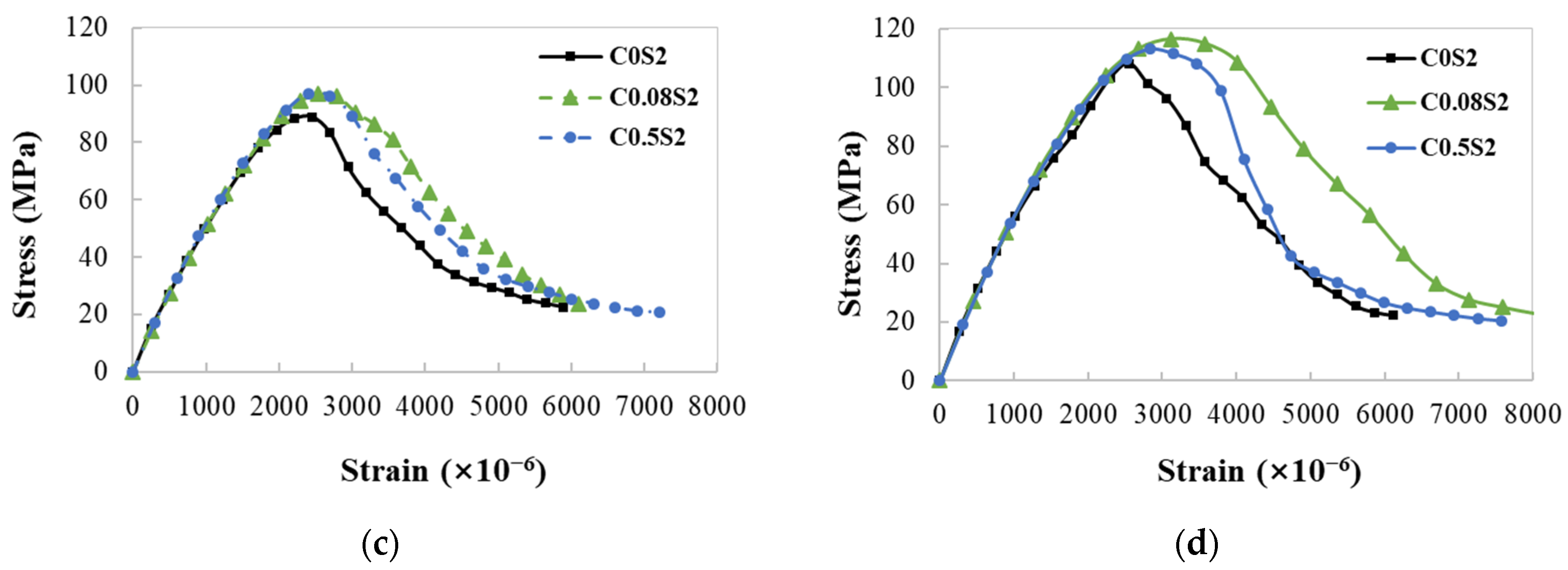
2.2.2. Stress–Strain Curve

According to the test results, the average stress–strain curves of each mixture were plotted, as illustrated in Figure 4.

The influence of CNT content on the stress–strain curves of specimens without steel fibers is limited, as depicted in Figure 4a,b. All of the specimens without steel fibers exhibited evident brittle failure, with a small descending section observed.

As shown in Figure 4c,d, specimens with 2% steel fibers exhibited ductile failure, indicating the significant influence of steel fibers on the stress–strain curve. The presence of CNTs can affect the descending section of the curve, and the inclusion of 0.08% CNTs resulted in a more gradual decline compared to specimens without CNTs and also those with 0.5% CNTs. This suggested that 0.08% CNTs can enhance the ductility, while excessive CNT contents can have adverse effects due to agglomeration [19]. The improvement of the descending section of the curve by CNTs can be attributed to their bridging effect on microcracks and the improvement in the microstructure and porosity of concrete [6].

2.2.3. Peak Stress and Peak Strain

Peak stress of different mixtures is compared, as shown in Figure 5a. Comparing specimens without steel fibers at 7 days of age, a 9% increase in peak stress was observed as the CNT content increased from 0 to 0.08%. With a further increase in CNT content to 0.5%, the peak stress was 5% higher than that of specimens without CNT. The addition of CNTs enhanced the peak stress, while excessive CNTs may weaken its effect on peak stress. This can be attributed to CNTs’ bridging effect for nano- and micron-scale cracks within the cement matrix. However, an excessive CNT content may lead to aggregation that weakens their strengthening effect. For specimens with 2% steel fibers, an increase in the CNT content from 0 to 0.08% resulted in elevation in peak stress by 11%. And as the CNT content further increased to 0.5%, there was an enhancement of 9% compared to specimens without CNT. Steel fibers can enhance the effect of CNTs on peak stress. The effect of CNTs and steel fibers on the peak stress remains consistent for the 28-day groups.

The peak strain of different mixtures is compared, as shown in Figure 5b. Comparing specimens without steel fibers at 7 days of age, the peak strain increased by 8% as the CNT content increased from 0 to 0.08%. With a further increase in the CNT content to 0.5%, the peak strain was 1% higher than that of specimens without CNT. Similar variations were observed for other groups with different ages and steel fiber contents. Similar to the pattern for peak stress, the addition of CNTs enhanced the peak strain, while excessive CNTs may weaken its effect on peak strain. In comparison with the C0S2, the peak strain of C0.08S2 and C0.5S2 increased by 10% and 8%, respectively. Similar to peak stress, steel fibers can enhance the effect of CNTs on peak strain.

The addition of steel fibers has a significant impact on the peak stress and peak strain, as shown in Figure 5. For instance, compared with C0.08S0, the peak stress of C0.08S2 increased by 50% at 7 days. This effect of steel fibers on peak stress was consistent for different ages and CNT contents. Similarly, there was also a noticeable improvement for the peak strain ranging from 33% to 48% for various age groups and CNT content levels as 2% steel fibers was added. This can be attributed to the ability of steel fibers to control crack development.

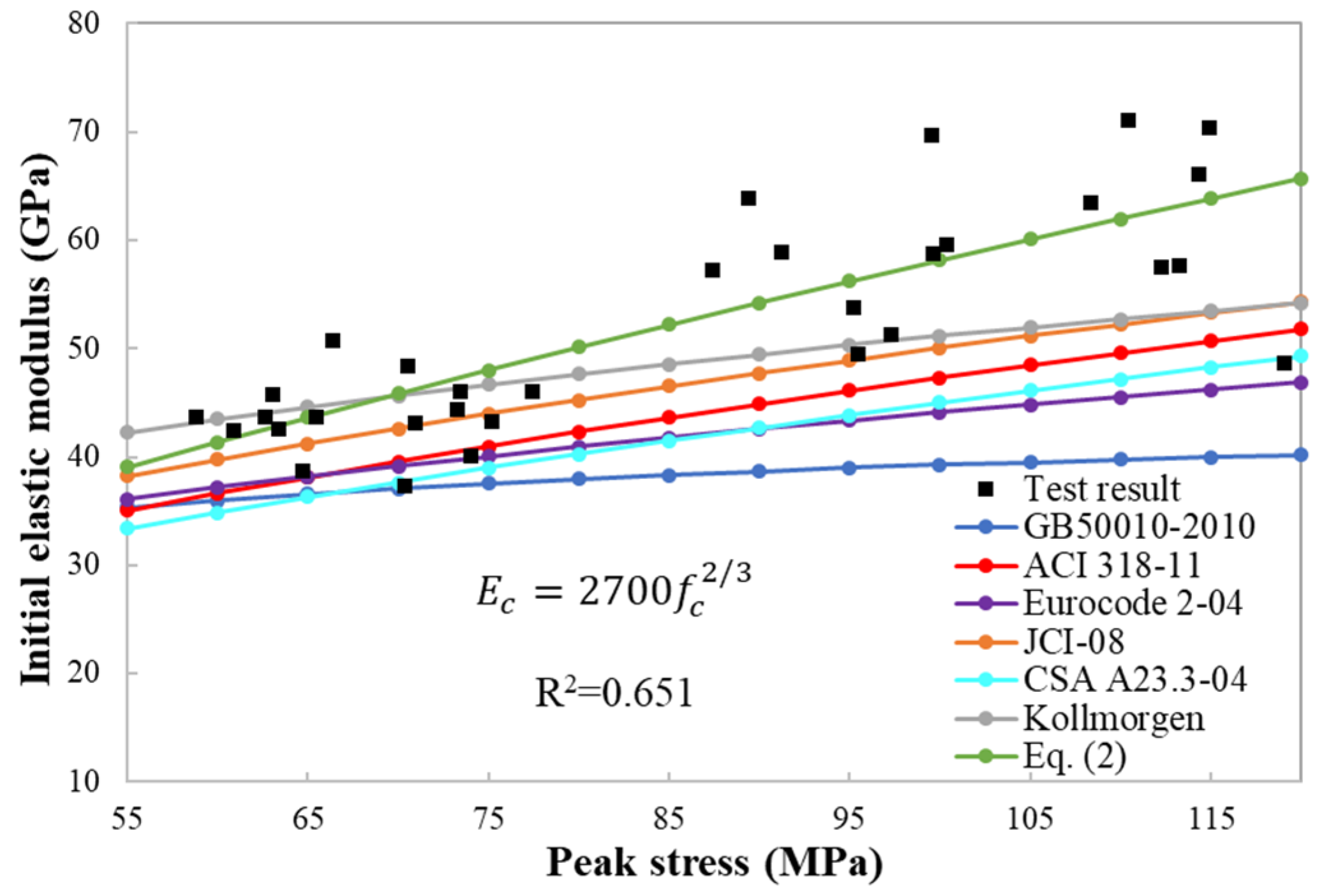
2.2.4. Elastic Modulus

The secant modulus at 80% of the peak stress in the stress–strain curve was calculated as the elastic modulus [39]. The average elastic modulus for each mixture proportion was calculated, as illustrated in Figure 6. Comparing different CNT contents, a small variation range of elastic modulus from −5% to 3% was observed, and there was no obvious variation pattern. CNTs’ bridging effect is for nanoscale and micron-scale cracks within the cement matrix, which have not yet formed and spread extensively at 80% of peak stress [39]. The addition of steel fibers enhanced the elastic modulus, with an increase ranging between 5% and 19%. The age exhibited no significant impact on elastic modulus.

2.2.5. Toughness Index

The toughness index, denoted as $T_r$, serves as an indicator for the ductility. It is determined as the ratio of the area enclosed by the stress–strain curve prior to a strain value of ${\epsilon }_{tr}=0.006$ and the coordinate axis and the rectangular area formed by the peak stress and ${\epsilon }_{tr}=0.006$, as shown in Figure 7, where $\sigma$ and $f_c$ represent the stress and peak stress, respectively.

The toughness index of different mix proportions was calculated, as illustrated in Figure 8. For mixtures without steel fibers, age and CNT content had no significant influence on the toughness index. For mixtures with 2% steel fibers, those with 0.08% CNTs exhibited the highest toughness index, which was 11% and 17% higher than those without CNTs at 7 days and 28 days of age, respectively. However, as the CNT content increased to 0.5%, the toughness index decreased and was 3% and 7% higher than those without CNTs. This suggests that CNTs can enhance the toughness index when steel fibers are used, and excessive amounts may diminish its effectiveness.

The toughness index of mixtures without steel fibers was less than 0.26, and it increased and ranged between 0.60 and 0.72 as 2% steel fibers were added. Steel fibers can significantly improve the toughness index by limiting crack propagation. Furthermore, the toughness index increased by 2% to 15% with the increase in age.

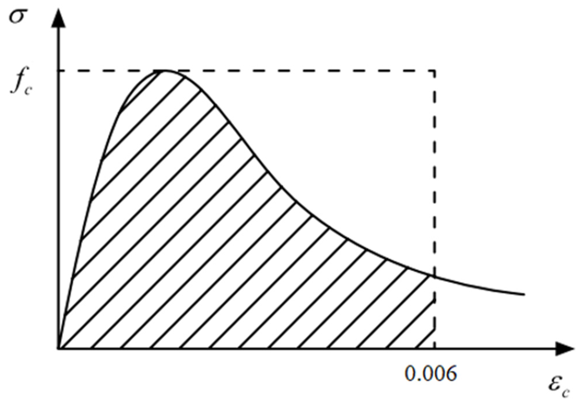
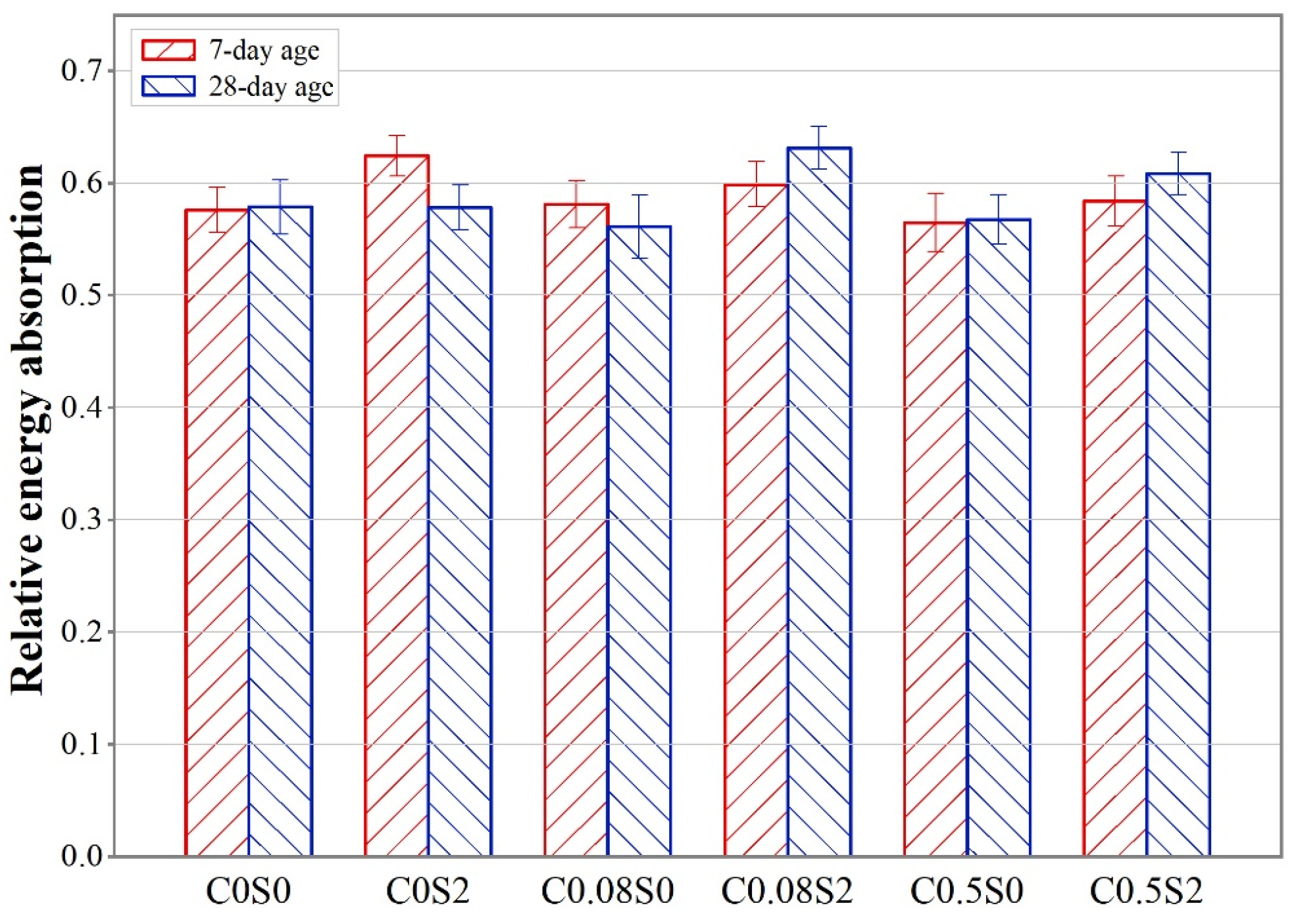
2.2.6. Relative Absorbed Energy

The energy absorption rate is defined as the area enclosed by the stress–strain curve and the transverse axis, spanning from the origin to the peak stress point [40]. The relative absorbed energy, denoted as $U_r$, refers to the energy absorption rate from the normalized stress–strain curve, which is obtained by dividing both stress and strain by their peak values. The brittleness of concrete can be represented by $U_r$. $U_r$ is 0.5 for a perfectly linear elastic material and 1.0 for a perfectly plastic material, as illustrated in Figure 9, where $\epsilon$ is the strain and ${\epsilon }_0$ is the peak strain.

The relative absorbed energy of different mix proportions was calculated, as illustrated in Figure 10. CNTs had negligible influence on the relative absorbed energy. Steel fibers can increase the relative absorbed energy, and the maximum increase was found at a CNT content of 0.08% and 28 days. No pattern can be found in the influence of age on the relative absorbed energy.

3. Theoretical Models

3.1. Theoretical Model for Peak Strain

The peak strain is a critical parameter that influences the characteristics of both the ascending and descending sections of the stress–strain curve.

Table 6. Theoretical equations for peak strain.

Literature	Theoretical Model
CEB/FIP [41]	${\epsilon }_0=0.0022$
Tadros [42]	${\epsilon }_0=\left(1.6+0.01f_c\right)\times {10}^{-3}$
Tomaszewicz [43]	${\epsilon }_0=700\times f_c^{0.31}\times {10}^{-6}$
Wee [44]	${\epsilon }_0=780\times f_c^{0.25}\times {10}^{-6}$
Lee [45]	${\epsilon }_0=f_c/\left(46.886+2.6f_c\right)$

presents the theoretical equations for peak strain proposed in various literatures.

Based on the test data in this study, a new theoretical model for peak strain is developed, as shown in Equation (1).

$${\epsilon }_0=120\times {f_c}^{2/3}\times {10}^{-6}$$

(1)

The test results of this study and the predicted results for the peak strain produced by different theoretical models are compared, as shown in Figure 11, and the model established in this study shows the best fit. The coefficient of determination (R²) of Equation (1) on the test result is 0.915. Equation (1) shows the best fit among the models.

3.2. Theoretical Model for Initial Elastic Modulus

The theoretical equations for the initial elastic modulus from previous studies are presented in

Table 7. Theoretical equations for initial elastic modulus.

Literature	Theoretical Model
GB50010–2010 [46]	$E_c=\frac{100000}{2.2+34.7/f_c}$
ACI 318-11 [47]	$E_c=4730\sqrt{f_c}$
Eurocode 2-04 [48]	$E_c=9500f_c^{1/3}$
JCI-08 [49]	$E_c=6300f_c^{0.45}$
CSA A23.3-04 [50]	$E_c=4500\sqrt{f_c}$
Kollmorgen [51]	$E_c=11800f_c^{1/3.14}$

$E_c$ represents the initial elastic modulus.

.

Based on the test data in this study, a new theoretical model for initial elastic modulus is proposed, as shown in Equation (2).

$$E_c=2700f_c^{2/3}$$

(2)

The test results of this study and the predicted results for the initial elastic modulus produced by different theoretical models are compared, as shown in Figure 12. The R² of Equation (2) on the test results of this study is 0.651. The model established in this study shows the best fit.

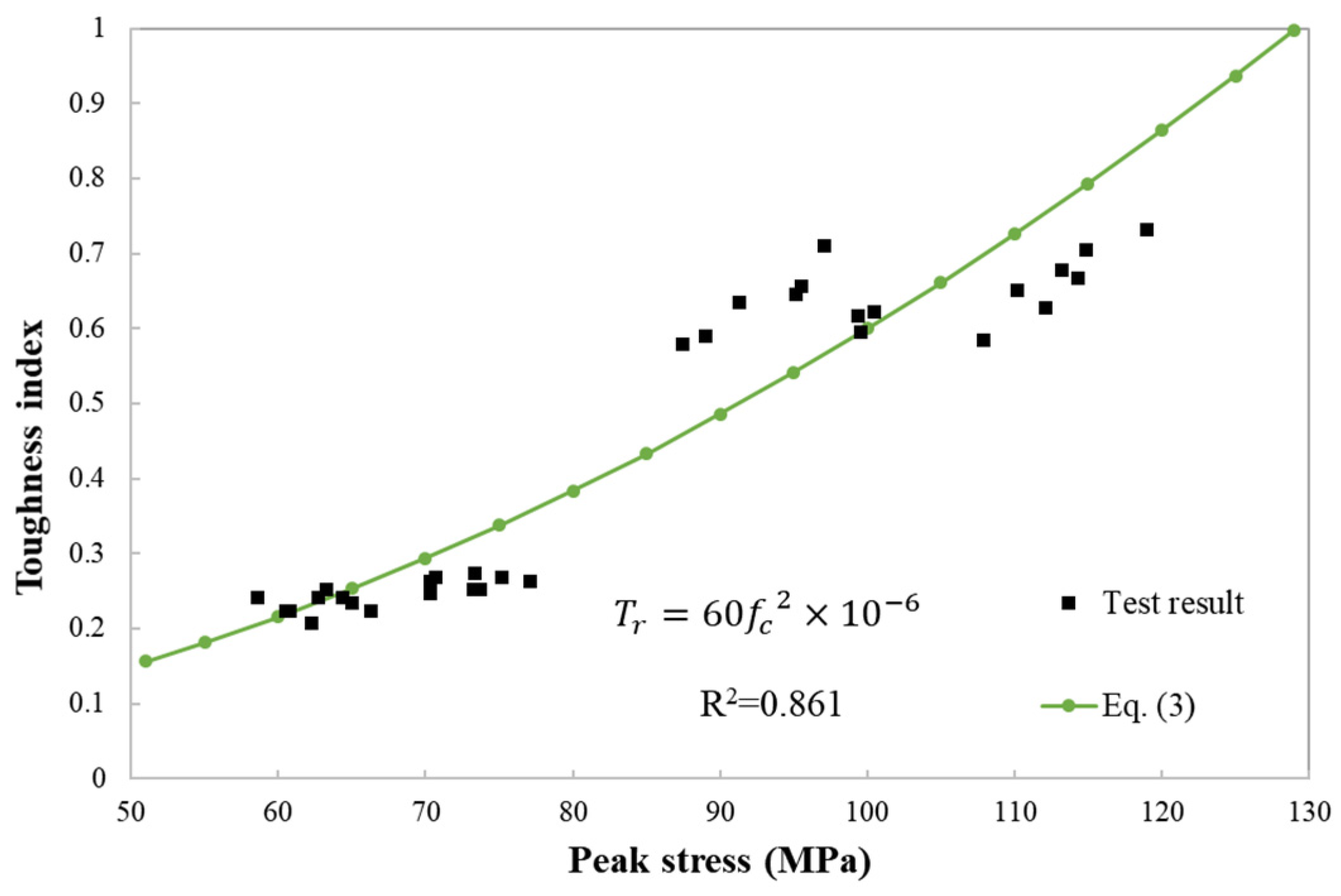
3.3. Theoretical Model for Toughness Index

Based on the test data in this study, a new theoretical model for toughness index is developed, as shown in Equation (3).

$$T_r=60{f_c}^2\times {10}^{-6}$$

(3)

The test results and predicted results for the toughness index are compared, as shown in Figure 13. The R² of Equation (3) is 0.861.

3.4. Theoretical Model for Relative Absorbed Energy

The theoretical equations for the relative absorbed energy from previous studies are presented in

Table 8. Theoretical equations for relative absorbed energy.

Literature	Theoretical Model
Tasdemir [40]	$U_r=1.038f_c^{-0.134}$
Nematzadeh [52]	$U_r=0.19f_c^{-0.17}$

.

Based on the experimental data in this study, a new theoretical model for relative absorbed energy is proposed, as shown in Equation (4).

$$U_r=0.38f_c^{0.1}$$

(4)

The test results and predicted results for the relative absorbed energy produced by different models are compared, as shown in Figure 14. The R² of Equation (4) is 0.723. Equation (4) shows the best fit.

3.5. Theoretical Model for Uniaxial Compressive Stress–Strain Curves

The theoretical models for stress–strain curves from the literature are presented in

Table 9. Theoretical models for stress–strain curves.

Literature	Theoretical Model
Smith and Young [53]	$y=x{e}^{1-x}$
Desayi and Krishnan [54]	$y=\frac{3x}{2+x^3}$
CEB/FIP [41]	$y=\frac{ax-x^2}{1+\left(a-2\right)x},a=\frac{E_c}{E_{sec}}$
Wee [44]	$y=\left\{\begin{array}{c}\frac{ax}{a-1+x^a},0\le x\le 1\\ \frac{kax}{ka-1+x^{na}},x>1\end{array},a=\frac{1}{1-\frac{E_{sec}}{E_c}},k={\left(\frac{50}{f_c}\right)}^3,n=\right.{\left(\frac{50}{f_c}\right)}^{1.3}$
GB50010-2010 [46]	$y=\left\{\begin{array}{c}\frac{ax}{a-1+x^a},0\le x\le 1\\ \frac{x}{k{\left(x-1\right)}^2+x},x>1\end{array},a=\frac{1}{1-\frac{E_{sec}}{E_c}},k=0.157\right.f_c^{0.785}-0.905$

$x=\frac{\epsilon }{{\epsilon }_0};y=\frac{\sigma }{f_c}$; and $E_{sec}$ is the secant modulus.

.

Based on the test data in this study, a new theoretical model is proposed.

A fourth-order polynomial is employed for the ascending section to consider the effect of CNTs and steel fibers, as shown in Equation (5).

$$y=ax+(4-3a)x^3+(2a-3)x^4$$

(5)

A fractional model is employed for the descending section, as shown in Equation (6).

$$y=\frac{x}{b{x}^3+(1-3b)x+2b}$$

(6)

To prevent overfitting, the coefficients $a$ and $b$ in the proposed model are taken as linear functions of the mass fraction of CNTs ($W_{cnt}$) and volume fraction of steel fibers ($V_{sf}$), as shown in Equations (7) and (8).

$$a={\alpha }_0+{\alpha }_1{W}_{cnt}+{\alpha }_2{V}_{sf}$$

(7)

$$b={\beta }_0+{\beta }_1{W}_{cnt}+{\beta }_2{V}_{sf}$$

(8)

By initializing the values of the linear coefficients ${\alpha }_0~{\alpha }_2$ and ${\beta }_0~{\beta }_2$ and applying the gradient descent method for the test results, the coefficients $a$ and $b$ for each mix proportion can be calculated, as presented in

Table 10. Coefficients $a$ and $b$ of the proposed model.

Age (Days)	Group	$\mathit{a}$	$\mathit{b}$
7	C0S0	1.162	0.256
	C0S2	1.402	0.384
	C0.08S0	1.239	0.235
	C0.08S2	1.415	0.335
	C0.5S0	1.076	0.281
	C0.5S2	1.320	0.371
28	C0S0	1.225	0.238
	C0S2	1.218	0.412
	C0.08S0	1.130	0.265
	C0.08S2	1.458	0.297
	C0.5S0	1.153	0.258
	C0.5S2	1.410	0.446

. The corresponding linear coefficients ${\alpha }_0~{\alpha }_2$ and ${\beta }_0~{\beta }_2$ can be determined based on Table 10, as listed in

Table 11. Coefficients ${\alpha }_0~{\alpha }_2$ and ${\beta }_0~{\beta }_2$ of the proposed model.

Coefficient	${\mathit{\alpha }}_0$	${\mathit{\alpha }}_1$	${\mathit{\alpha }}_2$	${\mathit{\beta }}_0$	${\mathit{\beta }}_1$	${\mathit{\beta }}_2$
value	1.18	−7.17	10.32	0.48	13.28	11.87

.

The test and predicted stress–strain curves produced by different theoretical models are compared, as shown in Figure 15 and Figure 16. The R² and root mean square error (RMSE) of different theoretical models are compared in Figure 17 and

Table 12. R² of prediction according to different theoretical models for stress–strain curves.

Model	7 Days Old						28 Days Old						Average
	C0S0	C0S2	C0.08 S0	C0.08 S2	C0.5S0	C0.5S2	C0S0	C0S2	C0.08 S0	C0.08 S2	C0.5S0	C0.5S2
Smith and Young [53]	0.748	0.052	0.764	0.440	0.701	0.352	0.767	0.079	0.717	0.484	0.744	0.101	0.496
Desayi and Krishnan [54]	0.956	0.550	0.962	0.822	0.933	0.785	0.961	0.598	0.936	0.808	0.951	0.568	0.819
CEB/FIP [41]	0.999	0.675	0.999	0.517	0.995	0.487	0.999	0.567	0.988	0.285	0.995	0.785	0.774
Wee [44]	0.997	0.903	0.996	0.862	0.985	0.897	0.991	0.841	0.970	0.799	0.982	0.799	0.919
GB50010-2010 [46]	0.997	0.991	0.996	0.892	0.985	0.949	0.991	0.939	0.970	0.947	0.982	0.966	0.967
Proposed model	0.999	0.912	0.999	0.995	0.995	0.991	0.999	0.945	0.995	0.987	0.999	0.935	0.979

and

Table 13. RMSE of prediction according to different theoretical models for stress–strain curves.

Model	7 Days Old						28 Days Old						Average
	C0S0	C0S2	C0.08 S0	C0.08 S2	C0.5S0	C0.5S2	C0S0	C0S2	C0.08 S0	C0.08 S2	C0.5S0	C0.5S2
Smith and Young [53]	9.54	24.06	9.85	20.81	10.68	22.41	10.90	29.02	12.97	27.06	12.14	33.64	18.59
Desayi and Krishnan [54]	4.01	16.58	3.96	11.72	5.05	12.91	4.44	19.17	6.18	16.49	5.34	23.33	10.77
CEB/FIP [41]	0.36	7.89	0.41	20.69	1.35	21.42	0.83	19.85	2.64	36.57	1.77	16.38	10.85
Wee [44]	1.08	7.71	1.23	10.35	2.42	8.92	2.08	12.07	4.25	16.89	3.21	15.92	7.18
GB50010-2010 [46]	1.08	2.30	1.23	9.12	2.42	6.26	2.08	7.49	4.25	8.67	3.21	6.59	4.56
Proposed model	0.65	7.34	0.66	1.98	1.42	2.36	0.66	7.07	1.75	4.22	0.78	9.06	3.16

. Furthermore, the R² and RMSE for the ascending and descending sections of the predicted stress–strain curves were calculated and compared, as depicted in Figure 18 and Figure 19 and

Table 14. R² of prediction according to different theoretical models for ascending section of stress–strain curves.

Model	7 Days Old						28 Days Old						Average
	C0S0	C0S2	C0.08 S0	C0.08 S2	C0.5S0	C0.5S2	C0S0	C0S2	C0.08 S0	C0.08 S2	C0.5S0	C0.5S2
Smith and Young [53]	0.748	0.898	0.764	0.845	0.701	0.819	0.767	0.779	0.717	0.927	0.744	0.874	0.799
Desayi and Krishnan [54]	0.956	0.997	0.962	0.985	0.933	0.973	0.961	0.954	0.936	0.999	0.951	0.991	0.967
CEB/FIP [41]	0.999	0.997	0.999	0.998	0.995	0.995	0.999	0.976	0.988	0.994	0.995	0.998	0.994
Wee [44]	0.997	0.999	0.996	0.987	0.985	0.981	0.991	0.945	0.970	0.999	0.982	0.986	0.985
GB50010-2010 [46]	0.997	0.999	0.996	0.987	0.985	0.981	0.991	0.945	0.970	0.999	0.982	0.986	0.985
Proposed model	0.999	0.997	0.999	0.999	0.995	0.995	0.999	0.981	0.995	0.993	0.999	0.998	0.996

,

Table 15. RMSE of prediction according to different theoretical models for ascending section of stress–strain curves.

Model	7 Days Old						28 Days Old						Average
	C0S0	C0S2	C0.08 S0	C0.08 S2	C0.5S0	C0.5S2	C0S0	C0S2	C0.08 S0	C0.08 S2	C0.5S0	C0.5S2
Smith and Young [53]	9.54	9.44	9.85	12.54	10.68	13.62	10.90	15.96	12.97	10.74	12.14	13.24	11.8
Desayi and Krishnan [54]	4.01	1.54	3.96	3.86	5.05	5.26	4.44	7.30	6.18	1.23	5.34	3.46	4.3
CEB/FIP [41]	0.36	1.72	0.41	1.38	1.35	2.33	0.83	5.29	2.64	3.05	1.77	1.61	1.89
Wee [44]	1.08	1.08	1.23	3.66	2.42	4.43	2.08	7.94	4.25	1.36	3.21	4.39	3.09
GB50010-2010 [46]	1.08	1.08	1.23	3.66	2.42	4.43	2.08	7.94	4.25	1.36	3.21	4.39	3.09
Proposed model	0.65	1.66	0.66	1.17	1.42	2.26	0.66	4.65	1.75	3.43	0.78	1.79	1.74

,

Table 16. R² of prediction according to different theoretical models for descending section of stress–strain curves.

Model	7 Days Old			28 Days Old			Average
	C0S2	C0.08 S2	C0.5S2	C0S2	C0.08 S2	C0.5S2
Smith and Young [53]	−0.981	0.062	0.097	−0.458	0.271	−0.371	−0.230
Desayi and Krishnan [54]	−0.005	0.663	0.675	0.313	0.715	0.303	0.444
CEB/FIP [41]	0.497	0.296	0.510	−2.486	−17.185	−0.599	−3.161
Wee [44]	0.783	0.739	0.850	0.765	0.701	0.682	0.753
GB50010-2010 [46]	0.982	0.801	0.933	0.943	0.922	0.954	0.923
Proposed model	0.807	0.991	0.992	0.919	0.985	0.896	0.932

and

Table 17. RMSE of prediction according to different theoretical models for descending section of stress–strain curves.

Model	7 Days Old			28 Days Old			Average
	C0S2	C0.08 S2	C0.5S2	C0S2	C0.08 S2	C0.5S2
Smith and Young [53]	29.99	24.63	25.31	34.89	31.07	40.72	31.1
Desayi and Krishnan [54]	21.36	14.77	15.18	23.95	19.42	29.04	20.62
CEB/FIP [41]	23.89	33.74	34.40	30.21	51.61	25.82	33.28
Wee [44]	9.92	12.99	10.32	14.02	19.89	19.60	14.45
GB50010-2010 [46]	2.82	11.35	6.88	6.88	10.17	7.47	7.59
Proposed model	9.37	2.35	2.34	8.21	4.41	11.24	6.32

.

As shown in Figure 15 and Figure 16, the model established in this study shows the best fit for most mixtures. The prediction provided by the proposed model has the highest R² and the lowest RMSE on average and also for most individual cases, as evident in Figure 17 and Table 12 and Table 13. For the ascending section, the models developed by Desayi and Krishnan [54], CEB/FIP [41], Wee [44], GB50010-2010 [46] and the one presented in this study show excellent fit, as evident in Figure 18 and Table 14 and Table 15. Among these five models, the proposed model has the highest R² and the lowest RMSE on average. For the descending section, only two models, the GB50010-2010 model [46] and that presented in this study, show good fit for all mixtures, as evident in Figure 19 and Table 16 and Table 17, and also the proposed model has the best fit for the descending section since it has the highest R² and the lowest RMSE on average and also in most cases. Thus, the theoretical model proposed here is the most accurate and can be selected.

4. Finite Element Analysis

4.1. General

Finite element analysis was conducted using the representative volume element (RVE) method. The software Ansys, version R18.0 was utilized. Steel fibers are distributed in a homogeneous RVE cylinder of Φ50 mm × 100 mm. The specimen consists of two components: steel fibers and RVE. The RVE is composed of a homogeneous cement-based material and distributed CNTs. Firstly, a 100 μm × 100 μm cube RVE was modeled as a composite material and its constitutive relationship was analyzed. Then, the cylinder specimen was modeled and the simulation results were compared with experimental data.

In the FE model, the CNTs and steel fibers are assumed to be distributed uniformly and randomly in the matrix, which was realized by the rand() function in Ansys. The total number of fibers is determined by dividing the overall fiber volume in the matrix by the volume of one individual fiber, as shown in Equation (9).

$$n=\left[\frac{V\times v_f}{v}\right]$$

(9)

where $n$ is the number of fibers, $\left[x\right]$ is the integer function, and $V$ is the volume of the matrix. For RVE, the matrix is a cube with side length of $100\mathsf{\mu }\mathrm{m}$, and for the specimen, the matrix is a cylinder of $\mathsf{\Phi }50\mathrm{m}\mathrm{m}\times 100\mathrm{m}\mathrm{m}.V_f$ is the volume fraction of the fiber, and $v$ is the volume of a single fiber. In this FE model, steel fibers and CNTs are regarded as slender round rods. The diameter and length of the steel fibers and CNTs are $d_{sf}=$ 0.22 mm, $l_{sf}=$ 13 mm, $d_{cnt}=$ 50 nm, $l_{cnt}=$ 15 μm, respectively. The distribution of CNTs in RVE and steel fibers in specimen was modelled, as shown in Figure 20 and Figure 21, respectively.

To enhance model convergence and computational efficiency, simplifications were implemented in this study. GO was solely employed as a surfactant and thus was not considered in modeling. The cement matrix in RVE was treated as a homogeneous entity with mechanical properties derived from control specimens without CNTs and steel fibers.

4.2. Modeling of RVE

4.2.1. Geometry and Material Models

A 100 μm cubic RVE matrix was simulated, and Solid65 unit was used. For the failure criterion, C1 was set to 0.5, C2 to 1.0, and C3 to −1, semi-brittle cracking behavior was considered for C9, and default values were used for other parameters. The multi-linear kinematic hardening model (KINH) was employed for the cement matrix, with the material properties determined by the test stress–strain curve of C0S0 specimens. CNTs within the RVE were simulated using Link10 elements and restricted to tension only. CNTs were considered as ideal elastic–plastic materials, and a bilinear kinematic model (BKIN) material model with an elastic modulus of 750 GPa and tensile strength of 50 GPa was adopted.

4.2.2. Meshing

The cement matrix had a partition density of 12 units along each side. Each CNT was divided into four segments. The meshing result of the RVE is illustrated in Figure 22.

4.2.3. Constraint and Loading

The CEINTF command was utilized to couple the cell nodes of CNTs and the cement matrix, with CNTs as the dense grid region and the cement matrix as the sparse grid region. A tolerance value of 25% (TOLER = 25%) was selected. All nodes on the bottom of the RVE cube were subjected to constraints in the X, Y, and Z directions. A displacement load was applied to the top surface. Force convergence criteria were employed with a convergence accuracy of 5%. The number of load steps was 1000.

4.3. Modeling of Specimens

4.3.1. Geometry and Material Models

The test specimen of Φ50 mm × 100 mm cylinder was modeled. The Link10 unit was employed for steel fibers, with only tension considered. The real constant of the Link10 unit was the cross-sectional area of steel fibers, 0.038 mm². The BKIN model was used for steel fibers, characterized by an elastic modulus of 200 GPa and a tensile strength of 2850 MPa.

4.3.2. Meshing

The steel fibers were meshed into two segments. The grid for the RVE matrix was a hexahedron, with a partition density of 20 units along the cylinder’s height and 24 units along the top and bottom surface circumferences. The meshing result is illustrated in Figure 23.

4.3.3. Constraints and Loading

The coupling between steel fibers and the RVE matrix was simulated through the CEINTF command, with the former considered as the dense grid region and the latter as the sparse one. A tolerance of 25% (TOLER = 25%) was selected. All element nodes on the bottom surface of the cylinder were subjected to constraints in the directions of X, Y, and Z, while a fixed vertical displacement load was applied to the top surface. Automatic load step adjustment was employed.

4.4. Results of FEA

4.4.1. Stress–Strain Curve

The stress–strain curves of C0.08S2 and C0.5S2 from the FE simulation are compared with the test results, as shown in Figure 24.

The stress–strain curves from the FE simulation exhibit good agreement with the measured curves in the ascending section, except that the FE curves show higher peak stress and peak strain values. For the descending section, enhanced ductility is demonstrated in the FE curves. These differences can be attributed to defects present in the test specimens compared with the ideal condition in the simulation. The actual effect of steel fibers on cracks is also limited compared with the ideal condition in FE modelling. Also, a simplification was made in the modelling, and refined models considering properties of CNTs at the nanoscale need be further studied.

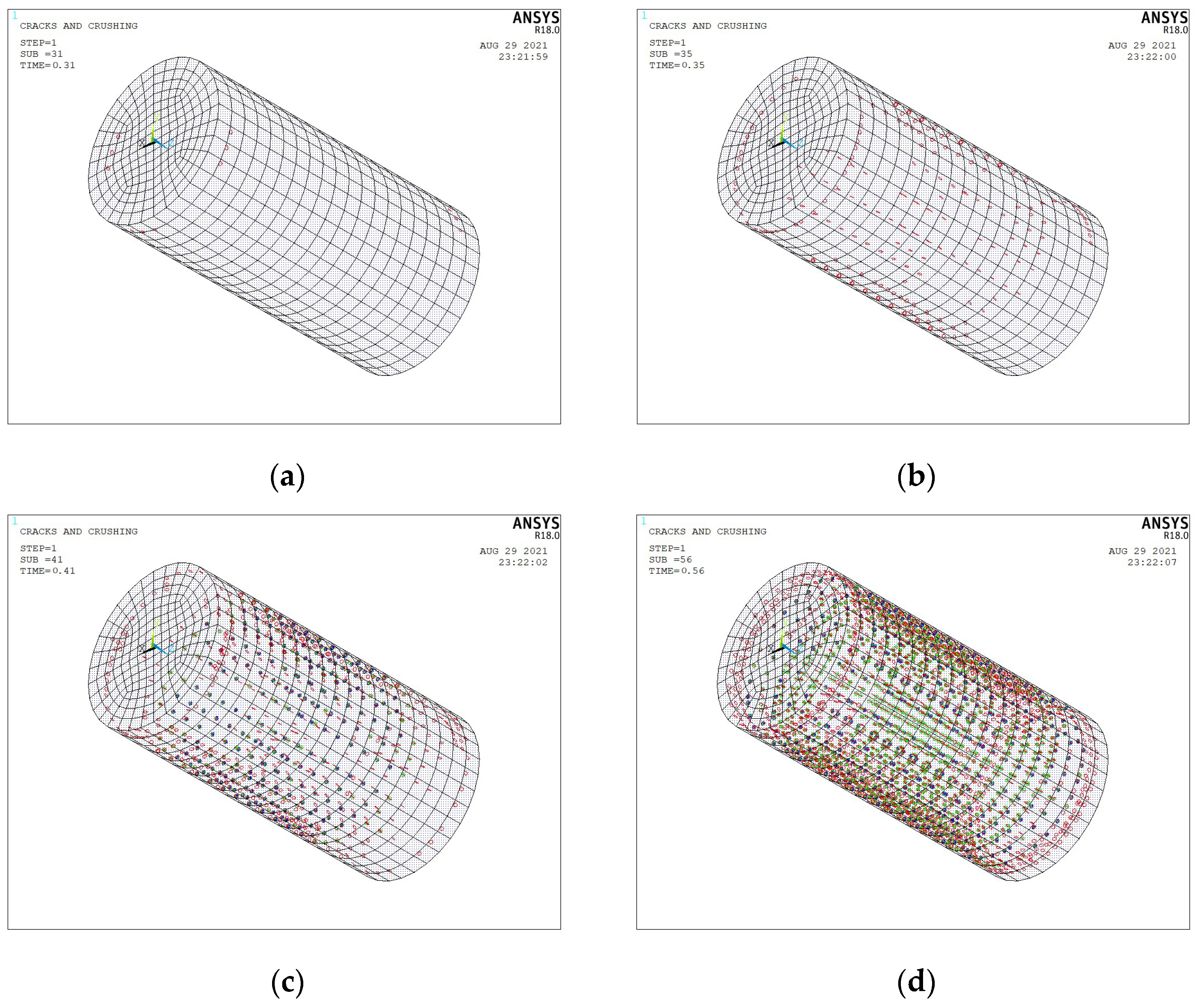
4.4.2. Crack Development

The crack development of the C0.08S2 specimen was analyzed using the FE modelling. The crack propagation under various load steps is shown Figure 25. The cracks were first observed after the 31st loading step near the top and bottom of the specimen, where displacement loads and constraint were applied. As the load increased, axial cracking on the side occurred, and previously observed cracks near the top and bottom developed. After the 41st loading step, cracks widely distributed on the surface of the specimen, which is consistent with the experiment.

5. Conclusions

The compressive properties of CNT-reinforced concrete were studied through an experimental investigation. The theoretical models of peak strain, elastic modulus, toughness index, relative absorbed energy and also compressive stress–strain curves of CNT-reinforced concrete were proposed. The following conclusions can be drawn:

(1)

CNT content had little influence on the failure process and elastic modulus. The incorporation of CNTs can enhance the peak stress and peak strain due to CNTs’ bridging effect for nano- and micron-scale cracks, while an excessive CNT content may weaken this effect due to CNTs’ aggregation. Steel fibers can enhance the effect of CNTs on peak stress and peak strain.

(2)

In the absence of steel fibers, CNTs had negligible influence on toughness index, while steel fibers can enhance the effect of CNTs on toughness index. Nevertheless, excessive CNTs diminished this enhancement effect.

(3)

Steel fibers can increase the peak stress, peak strain, elastic modulus, toughness index and relative absorbed energy of concrete, and can result in ductile failure.

(4)

Theoretical models for peak strain, initial elastic modulus, toughness index and relative absorbed energy were established. The models were in good agreement with experiment results.

(5)

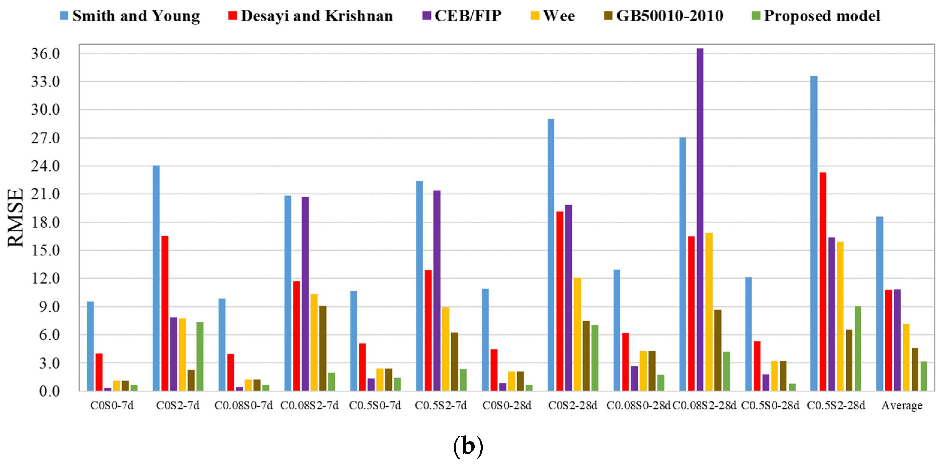
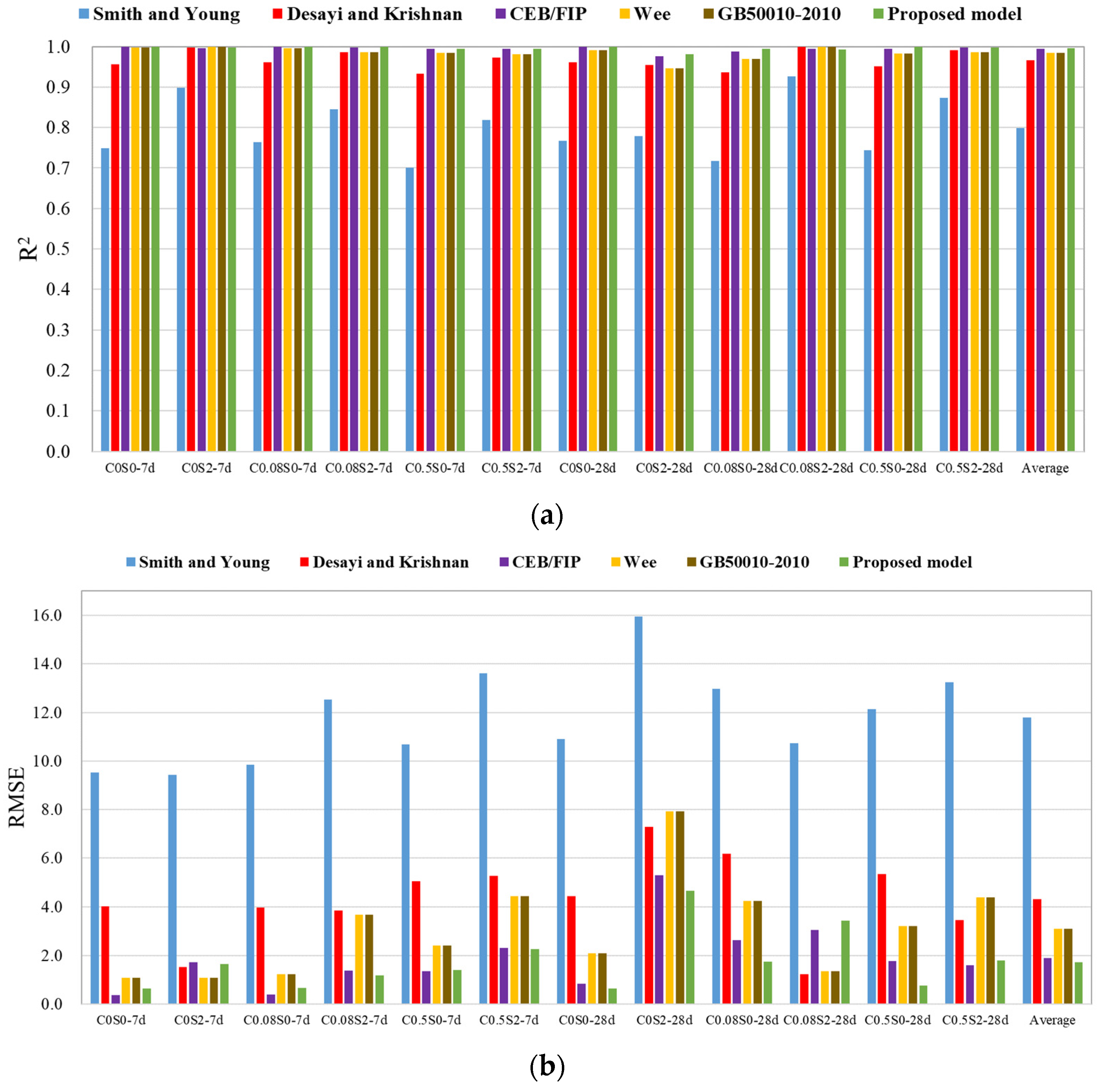
A theoretical model for the stress–strain curve of CNT-reinforced concrete was developed considering the content of CNTs and steel fibers. The proposed model demonstrated the best fit among the different theoretical models.

(6)

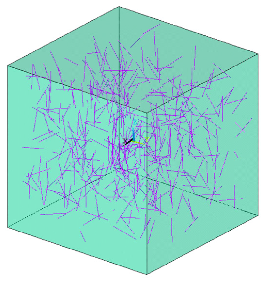
Considering the random distribution of CNTs and steel fibers, a simplified FE model was developed using the RVE method. The specimen was divided into two components: steel fibers and RVE with CNTs and cement-based material. There is agreement between the experimental and simulation results. The differences between the FE modelling and the experimental results can be attributed to defects in the test specimens compared with the ideal condition in the simulation. Refined models considering the properties of CNTs at the nanoscale need be further studied for better simulation accuracy.

(7)

Due to the high cost of the materials, the mixture proportions considered and tests performed in this study were limited. More tests are needed to study the influence of CNT on concrete properties. Additionally, a simplified FE model was developed, and refined FE models considering properties of CNTs at the nanoscale need be further studied for better simulation accuracy.

References

1. Yoo, D.Y.; Shin, H.O.; Yang, J.M.; Yoon, Y.S. Material and bond properties of ultra high performance fiber reinforced concrete with micro steel fibers. Compos. Part B Eng. 2014, 58, 122–133. [Google Scholar] [CrossRef]
2. Ates, A. Mechanical properties of sandy soils reinforced with cement and randomly distributed glass fibers (GRC). Compos. Part B Eng. 2016, 96, 295–304. [Google Scholar] [CrossRef]
3. Hambach, M.; Moeller, H.; Neumann, T.; Volkmer, D. Carbon fiber reinforced cement-based composites as smart floor heating materials. Compos. Part B Eng. 2016, 90, 465–470. [Google Scholar] [CrossRef]
4. Shah, S.P.; Ouyang, C. Mechanical behavior of fiber-reinforced cement-based composites. J. Am. Ceram. Soc. 1991, 74, 2727–2738. [Google Scholar] [CrossRef]
5. Tyson, B.M.; Abu Al-Rub, R.K.; Yazdanbakhsh, A.; Grasley, Z. Carbon Nanotubes and Carbon Nanofibers for Enhancing the Mechanical Properties of Nanocomposite Cementitious Materials. J. Mater. Civ. Eng. 2011, 23, 1028–1035. [Google Scholar] [CrossRef]
6. Pacheco-Torgal, F.; Jalali, S. Nanotechnology: Advantages and drawbacks in the field of construction and building materials. Constr. Build. Mater. 2011, 25, 582–590. [Google Scholar] [CrossRef]
7. Makar, J.; Beaudoin, J. Carbon nanotubes and their application in the construction industry. In Proceedings of the 1st International Symposium on Nanotechnology in Construction, Paisley, Scotland, 23–25 June 2003; Bartos, P., Ed.; [Google Scholar]
8. Wong, I.S. Effects of Ultra-Low Concentrations of Nanomaterials on the Piezoresistivity of Cementitious Composites. Master’s Thesis, University of California, Berkeley, CA, USA, 2015. [Google Scholar]
9. Han, B.; Sun, S.; Ding, S.; Zhang, L.; Yu, X.; Ou, J. Review of nanocarbon-engineered multifunctional cementitious composites. Compos. Part A Appl. Sci. Manuf. 2015, 70, 69–81. [Google Scholar] [CrossRef]
10. Onaizi, A.M.; Huseien, G.F.; Lim, N.H.A.S.; Amran, M.; Samadi, M. Effect of nanomaterials inclusion on sustainability of cement-based concretes: A comprehensive review. Constr. Build. Mater. 2021, 306, 124850. [Google Scholar] [CrossRef]
11. Jiang, Z.; Sevim, O.; Ozbulut, O.E. Mechanical properties of graphene nanoplatelets-reinforced concrete prepared with different dispersion techniques. Constr. Build. Mater. 2021, 303, 124472. [Google Scholar] [CrossRef]
12. Kaushik, B.K.; Goel, S.; Rauthan, G. Future VLSI interconnects: Optical fiber or carbon nanotube—A review. Microelectron. Int. 2007, 24, 53–63. [Google Scholar] [CrossRef]
13. Yu, M. Strength and breaking mechanism of multiwalled carbon nanotubes under tensile load. Science 2000, 287, 637–640. [Google Scholar] [CrossRef] [PubMed]
14. Walters, D.A.; Ericson, L.M.; Casavant, M.J.; Liu, J.; Colbert, D.T.; Smith, K.A.; Smalley, R.E. Elastic strain of freely suspended single-wall carbon nanotube ropes. Appl. Phys. Lett. 1999, 74, 3803–3805. [Google Scholar] [CrossRef]
15. Zhang, P.; Su, J.; Guo, J.; Hu, S. Influence of carbon nanotube on properties of concrete: A review. Constr. Build. Mater. 2023, 369, 13038. [Google Scholar] [CrossRef]
16. Jiang, S.; Zhou, D.C.; Zhang, L.Q.; Ouyang, J.; Yu, X.; Cui, X.; Han, B.G. Comparison of compressive strength and electrical resistivity of cementitious composites with different nano- and micro-fillers. Arch. Civ. Mech. Eng. 2018, 18, 60–68. [Google Scholar] [CrossRef]
17. Kumar, S.; Kolay, P.; Malla, S.; Mishra, S. Effect of multi-walled carbon nano tubes (CNT) on mechanical strength of cement paste. J. Mater. Civ. Eng. 2012, 24, 84–91. [Google Scholar] [CrossRef]
18. Chaipanich, A.; Rianyoi, R.; Nochaiya, T. The effect of carbon nanotubes and silica fume on compressive strength and flexural strength of cement mortars. Mater. Today Proc. 2017, 4, 6065–6071. [Google Scholar] [CrossRef]
19. Gillani, S.S.U.; Khitab, A.; Ahmad, S.; Khushnood, R.A.; Ferro, G.A.; Kazmi, S.M.S.; Qureshi, L.A.; Restuccia, L. Improving the mechanical performance of cement composites by carbon nanotubes addition. Procedia Struct. Integr. 2017, 3, 11–17. [Google Scholar] [CrossRef]
20. Xu, S.; Liu, J.; Li, Q. Mechanical properties and microstructure of multi-walled carbon nanotube-reinforced cement paste. Constr. Build. Mater. 2015, 76, 16–23. [Google Scholar] [CrossRef]
21. Wang, B.; Han, Y.; Liu, S. Effect of highly dispersed carbon nanotubes on the flexural toughness of cement-based composites. Constr. Build. Mater. 2013, 46, 8–12. [Google Scholar] [CrossRef]
22. Lourie, O.; Cox, D.; Wagner, H. Buckling and collapse of embedded carbon nanotubes. Phys. Rev. Lett. 1998, 81, 1638. [Google Scholar] [CrossRef]
23. Szleifer, I.; Yerushalmi-Rozen, R. Polymers and carbon nanotubes—Dimensionality, interactions and nanotechnology. Polymer 2005, 46, 7803–7818. [Google Scholar] [CrossRef]
24. Han, B.G.; Yu, X.; Ou, J.P. Multifunctional and smart carbon nanotube reinforced cement-based materials. In Nanotechnology in Civil Infrastructure: A Paradigm Shift; Springer: Berlin/Heidelberg, Germany, 2011; pp. 1–47. [Google Scholar]
25. Lu, Z.; Hou, D.; Meng, L.; Sun, G.; Lu, C.; Li, Z. Mechanism of cement paste reinforced by graphene oxide/carbon nanotubes composites with enhanced mechanical properties. RSC Adv. 2015, 5, 100598–100605. [Google Scholar] [CrossRef]
26. Qiu, L.; Yang, X.; Gou, X.; Yang, W.; Ma, Z.; Wallace, G.G.; Li, D. Dispersing Carbon Nanotubes with Graphene Oxide in Water and Synergistic Effects between Graphene Derivatives. Chem.-A Eur. J. 2010, 16, 10653–10658. [Google Scholar] [CrossRef] [PubMed]
27. Parveen, S.; Rana, S.; Fangueiro, R. A review on nanomaterial dispersion, microstructure, and mechanical properties of carbon nanotube and nanofiber reinforced cementitious composites. J. Nanomater. 2013, 2013, 3271–3283. [Google Scholar] [CrossRef]
28. Nochaiya, T.; Chaipanich, A. Behavior of multi-walled carbon nanotubes on the porosity and microstructure of cement-based materials. Appl. Surf. Sci. 2011, 257, 1941–1945. [Google Scholar] [CrossRef]
29. Li, G.Y.; Wang, P.M.; Zhao, X.H. Mechanical behavior and microstructure of cement composites incorporating surface-treated multi-walled carbon nanotubes. Carbon 2005, 43, 1239–1245. [Google Scholar] [CrossRef]
30. Musso, S.; Tulliani, J.M.; Ferro, G.; Tagliaferro, A. Influence of carbon nanotubes structure on the mechanical behavior of cement composites. Compos. Sci. Technol. 2009, 69, 1985–1990. [Google Scholar] [CrossRef]
31. Abu Al-Rub, R.K.; Ashour, A.I.; Tyson, B.M. On the aspect ratio effect of multi-walled carbon nanotube reinforcements on the mechanical properties of cementitious nanocomposites. Constr. Build. Mater. 2012, 35, 647–655. [Google Scholar] [CrossRef]
32. Konsta-Gdoutos, M.S.; Metaxa, Z.S.; Shah, S.P. Highly dispersed carbon nanotube reinforced cement based materials. Cem. Concr. Res. 2010, 40, 1052–1059. [Google Scholar] [CrossRef]
33. Luo, J.L.; Duan, Z.D.; Li, H. The influence of surfactants on the processing of multi-walled carbon nanotubes in reinforced cement matrix composites. Phys. Status Solidi A-Appl. Mater. Sci. 2009, 206, 2783–2790. [Google Scholar] [CrossRef]
34. Collins, F.; Lambert, J.; Duan, W.H. The influences of admixtures on the dispersion, workability, and strength of carbon nanotube-OPC paste mixtures. Cem. Concr. Compos. 2012, 34, 201–207. [Google Scholar] [CrossRef]
35. Cwirzen, A.; Habermehl-Cwirzen, K.; Penttala, V. Surface decoration of carbon nanotubes and mechanical properties of cement/carbon nanotube composites. Adv. Cem. Res. 2017, 29, 65–73. [Google Scholar] [CrossRef]
36. ASTM C39/C39M-17; Standard Test Method for Compressive Strength of Cylindrical Concrete Specimens. ASTM International: West Conshohocken, PA, USA, 2017.
37. ASTM C31/C31M-03; Standard Practice for Making and Curing Concrete Test Specimens in the Field. ASTM International: West Conshohocken, PA, USA, 2003.
38. ASTM C192/C192M-16a; Standard Practice for Making and Curing Concrete Test Specimens in the ASTM Laboratory. ASTM International: West Conshohocken, PA, USA, 2016.
39. Jin, L.; Yu, W.X.; Li, D.; Du, X.L. Numerical and theoretical investigation on the size effect of concrete compressive strength considering the maximum aggregate size. Int. J. Mech. Sci. 2021, 192, 106130. [Google Scholar] [CrossRef]
40. Tasdemir, M.A.; Tasdemir, C.; Akyüz, S.; Jefferson, A.D.; Lydon, F.D.; Barr, B.I.G. Evaluation of Strains at Peak Stresses in Concrete: A Three-Phase Composite Model Approach. Cem. Concr. Compos. 1998, 20, 301–318. [Google Scholar] [CrossRef]
41. Comite Euro-International du Benton (CEB). CEB Model Code 90; Bulletin D’information: Paris, France, 1990; No. 203. [Google Scholar]
42. Tadros, G.S. Plastic Rotation of Reinforced Concrete Members Subjected to Bending, Axial Load and Shear. Ph.D. Thesis, ADV DEG, Civil Engineering University of Calgary, Calgary, AB, Canada, 1970. [Google Scholar]
43. Tomaszewicz, A. Betongens Arbeidsdiagram; SINTEF Rep. No. STF 65A84605; The Foundation for Industrial and Technical Research: Trondheim, Norway, 1984. [Google Scholar]
44. Wee, T.H.; Chin, M.S.; Mansur, M.A. Stress-strain relationship of high-strength concrete in compression. J. Mater. Civ. Eng. 1996, 8, 70–76. [Google Scholar] [CrossRef]
45. Lee, I. Complete Stress-Strain Characteristics of High Performance Concrete. Ph.D. Thesis, New Jersey Institute of Technology, Newark, NJ, USA, 2002. [Google Scholar]
46. GB 50010-2010; Code for Design of Concrete Structures. National Standard of the People’s Republic of China: Beijing, China, 2010.
47. ACI 318-11; Building Code Requirements for Structural Concrete and Commentary, PCA Notes on ACI 318-11: With Design Applications. ACI International: Farmington Hills, MI, USA, 2011.
48. Comité Européen de Normalisation. Eurocode 2: Design of Concrete Structures: Part 1-1: General Rules and Rules for Buildings; British Standards Institution: London, UK, 2004. [Google Scholar]
49. Japanese Civil Institute. Guidelines for Control of Cracking of Mass Concrete; Japan Concrete Institute: Tokyo, Japan, 2008. [Google Scholar]
50. Canadian Standard, CSA, A23.3-04; Design of Concrete Structures. Canadian Standard Association: Toronto, ON, Canada, 2004.
51. Kollmorgen, G.A. Impact of Age and Size on the Mechanical Behavior of an Ultra High Performance Concrete. Master’s Thesis, Michigan Technological University, Houghton, MI, USA, 2004. [Google Scholar]
52. Nematzadeh, M.; Salari, A.; Ghadami, J.; Naghipour, M. Stress-strain behavior of freshly compressed concrete under axial compression with a practical equation. Constr. Build. Mater. 2016, 115, 402–423. [Google Scholar] [CrossRef]
53. Smith, G.M.; Young, L.E. Ultimate theory in flexure by exponential function. ACI J. Proc. 1955, 52, 349–359. [Google Scholar]
54. Desayi, P.; Krishnan, S. Equation for the Stress-Strain Curve of Concrete. ACI J. Proc. 1964, 61, 345–350. [Google Scholar]
Figure 1. SWCNT and MWCNT [7]: (a) SWCNT; (b) MWCNT.
Buildings 14 00418 g001
Figure 2. Test setup.
Buildings 14 00418 g002
Figure 3. Failure modes of specimens at 7 days of age: (a) C0S0; (b) C0.08S0; (c) C0.5S0; (d) C0.5S2.
Buildings 14 00418 g003
Figure 4. Stress–strain curves of different mixture proportions: (a) no steel fibers at 7 d; (b) no steel fibers at 28 d; (c) 2% steel fibers at 7 d; (d) 2% steel fibers at 28 d.
Buildings 14 00418 g004aBuildings 14 00418 g004b
Figure 5. Peak stress and peak strain of different mixture proportions: (a) peak stress; (b) peak strain.
Buildings 14 00418 g005
Figure 6. Elastic modulus of different mixture proportions.
Buildings 14 00418 g006
Figure 7. Calculation of toughness index.
Buildings 14 00418 g007
Figure 8. Toughness index of different mixture proportions.
Buildings 14 00418 g008
Figure 9. Calculation of relative absorbed energy: (a) perfectly linear elastic material; (b) perfectly plastic material.
Buildings 14 00418 g009
Figure 10. Relative absorbed energy of different mixture proportions.
Buildings 14 00418 g010
Figure 11. Test results and predicted results for the peak strain produced by different theoretical models [41,42,43,44,45].
Buildings 14 00418 g011
Figure 12. Test results and predicted results for the initial elastic modulus produced by different theoretical models [46,47,48,49,50,51].
Buildings 14 00418 g012
Figure 13. Test results and predicted results for the toughness index.
Buildings 14 00418 g013
Figure 14. Test results and predicted results for the relative absorbed energy produced by different theoretical models [40,52].
Buildings 14 00418 g014
Figure 15. Test and predicted stress–strain curves at 7 days produced by different theoretical models [41,44,46,53,54]: (a) C0S0; (b) C0S2; (c) C0.08S0; (d) C0.08S2; (e) C0.5S0; (f) C0.5S2.
Buildings 14 00418 g015aBuildings 14 00418 g015b
Figure 16. Test and predicted stress–strain curves at 28 days produced by different theoretical models [41,44,46,53,54]: (a) C0S0; (b) C0S2; (c) C0.08S0; (d) C0.08S2; (e) C0.5S0; (f) C0.5S2.
Buildings 14 00418 g016aBuildings 14 00418 g016b
Figure 17. The R2 and RMSE of prediction according to different theoretical models for stress–strain curves [41,44,46,53,54]: (a) R2; (b) RMSE.
Buildings 14 00418 g017aBuildings 14 00418 g017b
Figure 18. The R2 and RMSE of prediction according to different theoretical models for the ascending section of stress–strain curves [41,44,46,53,54]: (a) R2; (b) RMSE.
Buildings 14 00418 g018
Figure 19. The R2 and RMSE of prediction according to different theoretical models for the descending section of stress–strain curves [41,44,46,53,54]: (a) R2; (b) RMSE.
Buildings 14 00418 g019
Figure 20. Distribution of CNTs (0.5%) in RVE.
Buildings 14 00418 g020
Figure 21. Distribution of steel fibers (2%) in the specimen.
Buildings 14 00418 g021
Figure 22. Meshing of RVE: (a) cement matrix; (b) CNTs (0.5%).
Buildings 14 00418 g022
Figure 23. Meshing of the specimen: (a) RVE matrix; (b) steel fibers (2%).
Buildings 14 00418 g023
Figure 24. Stress–strain curves from experiment and FE modelling: (a) C0.08S2; (b) C0.5S2.
Buildings 14 00418 g024
Figure 25. Crack development of the C0.08S2 specimen at different load steps in the FE model: (a) the 31st step; (b) the 35th step; (c) the 41st step; (d) the 56th step.
Buildings 14 00418 g025