International Comparison of Weather and Emission Predictive Building Control

Abstract

Building operational energy alone accounts for 28% of global carbon emissions. A sustainable building operation promises enormous savings, especially under the increasing concern of climate change and the rising trends of the digitalization and electrification of buildings. Intelligent control strategies play a crucial role in building systems and electrical energy grids to reach the EU goal of carbon neutrality in 2050 and to manage the rising availability of regenerative energy. This study aims to prove that one can create energy and emission savings with simple weather and emission predictive control (WEPC). Furthermore, this should prove that the simplicity of this approach is key for the applicability of this concept in the built world. A thermodynamic simulation (TRNSYS) evaluates the performance of different variants. The parametrical study varies building construction, location, weather, and emission data and gives an outlook for 2050. The study showcases five different climate locations and reveals heating and cooling energy savings of up to 50 kWh/(m²a) and emission savings between 5 and 25% for various building types without harming thermal comfort. This endorses the initial statement to simplify building energy concepts. Furthermore, it proposes preventing energy designers from overoptimizing buildings with technology as the solution to a climate-responsible energy concept.

1. Introduction

With climate neutrality being the EU’s goal in 2050, dramatic changes in the building industry are more than necessary, as the sector accounts for 40% of global carbon emissions [1]. The building operation alone is responsible for 28% [2]. In addition to the renovation strategies addressing the building envelopes, the modern approach to electrifying the building operation using heat pumps promises energy savings and, thus, CO₂ reductions. However, not only the building but also the mobility industry is increasingly focusing on electric concepts. Combined with the increasing fluctuation in electrical energy production based on the rising share of regenerative sources in the grid, intelligent control strategies are essential [3]. Today, additional energy will be provided by a power plant that still has spare capacity. These marginal power plants usually run on fossil fuels and emit a high amount of CO₂ [4].

Various concepts and data-driven control strategies, based on model predictive control, deep learning, weather forecast, or artificial intelligence, have been developed in the last decade, outlining energy- and CO₂-saving potentials [3,5,6,7,8]. Thereby, a few hurdles make it difficult to transform the concept into practice: data-intense algorithms, the creation of digital twins, or the necessity of highly educated employees to manage building technology. Standard building users or building operation managers are not data science experts and cannot apply these concepts to the built world. In international norms and codes, it is standard to consider a continuous static emission factor over the year. Several studies show that this leads to substantial rebound effects and does not represent reality. These studies ask for an hourly-based, dynamic emission value to address the fluctuation in the emissions in the electrical energy grid in a correct manner and to open up the potential for intelligent control strategies [3,9,10,11]. As this phenomenon depends on the electrical energy grid and the local weather conditions of a building, this is not only a problem for Germany but demands international application, as presented in this contextual parametric study.

This introduction further outlines the objective of the topic by formulating an overall hypothesis and linked research questions. Further, the methodology explains the simulation structure and revises two previous individual simulation approaches that form its basis. The following section Data and Methods describes the simulation base case model and the considered simulation variants for the parameter study. Finally, this section illustrates the weather and the characteristics of the emission data of the electrical grid for all five climate locations. Section 3, Results and Evaluation, presents the main findings of the thermal simulations and prepares for Section 4 Discussion and 5 Conclusion, where the initially stated hypothesis and research questions are evaluated.

1.1. Objective

As previously outlined, the electric demand in the building and the electricity grid continues to play a significant role in mitigating the effects of ongoing climate change. Nevertheless, with these sustainable transformations in energy supply for buildings and mobility (e.g., using heat pumps or electric cars), the overall demand for electrical energy rises significantly and becomes less predictable. To account for this scenario, the share of renewable energy must be significantly increased. But, for renewable energies, especially for photovoltaics (PVs), the electrical output depends on the local weather conditions, leading to prominent fluctuations in supply. This situation plays a significant role in the transformation process of the overall goal of the European Union of climate neutrality in 2050 [12]. This momentum is further transformed into German law, called the Generation contract [12,13]. This leads to the main idea of this paper, which demands a simple approach, performing a weather-and-emission predictive control of building technology. This paper presents a parametric study of five different locations, considering the individual climate and electricity emission conditions. To evaluate the impact of the concept, this paper addresses the following hypothesis and the connected research questions for each climate location:

The simple concept of weather-and-emission predictive control improves the overall energy performance and emission balance of a building without harming thermal comfort.

• What impact does the insulation and thermal mass have on the performance of the WEPC?
• How does a photovoltaic system impact the emission balance using the WEPC with thermal and electrical storage?
• Does the WEPC improve a room’s energy performance and CO₂ balance without compromising thermal comfort?
• How does the WEPC perform in 2050, considering future weather and emission data that account for an increased share of regenerative energies?

1.2. Methodology

This study combines the concepts of a series of papers and summarizes the overall approach. The first paper validated the thermodynamic model using an in situ measurement room [14]. Both the second and third papers outlined a concept focusing on the impact of a CO₂-optimized and weather predictive control [3,15]. This paper combines the two building control approaches into one simulation model using a validated thermodynamic simulation model. Based on these assumptions, a parametric study focuses on the impact of thermal mass, insulation, and a thermal and electrical storage system with PV. This parametric study is completed with an outlook on the behavior of control strategies in the future, assuming weather and emission data for 2050. These parameters are varied for five different climate locations to evaluate the effect on an international level. Finally, based on this parametric study, the initial research question and the linked hypotheses are answered. The following two sections review the overall approaches of the previous studies and outline the main findings of the two individual concepts.

1.2.1. Review—Impact of a Dynamic Emission Factor Optimized Control

With the electrification of energy production for buildings and mobility, the electricity grid’s emission factor (EF) plays a significant role in evaluating sustainability. Currently, the calculation of the CO₂ emission footprint focuses on static EFs. However, with the increasing fluctuation in the electrical grid on both the demand and supply side, the EF behavior becomes more and more dynamic. On the one side, this enhances the criticism of the miscalculation of emission footprints. On the other side, it opens up enormous potential for CO₂ savings, going hand in hand with smart control strategies. The dynamic emissions are calculated accordingly to the following equation:

$${\mathrm{E}}_{\mathrm{d}\mathrm{y}\mathrm{n}}=\sum _{t=1}^{8760}\left(p_{net}\left(t\right)·\frac{ef\left(t\right)}{1000}\right)$$

(1)

This study suggests that the dynamic balance for different building system variants deviates considerably from the static approach and opens possibilities to decrease emissions [3]. The research gap, founded on the literature review, outlines that the emission balance of a building operation changes when using dynamic EFs that map fluctuations at an hourly resolution. The results show that the dynamic balance approach deviates from the static one. Further, this paper’s predictive loading strategies outperform standard control strategies. This increases with building systems with inert storage units and/or PV integration, where charging time plays a significant role. As this paper focuses on a German location, the authors motivate further research on an international level with different electricity grids and weather conditions. They add that a broader view of the concept, such as the predictive control of variables focusing on energy efficiency, could result in new possibilities and transform buildings in thermal and emission short-term storage.

1.2.2. Review—Impact of a Weather Predictive Control

With the ongoing digitalization and electrification trends in Germany, using electrical heat pumps, the energy supply for buildings follows that pass. This leads to the demand for smart control strategies, especially with inert building systems. This study deals with a simple weather predictive control (WPC) approach, using thermally activated building systems (TABSs) to create energy savings while providing thermal comfort [15]. The research gap of this paper is based on the phenomena of the performance gap [16], as well as on the energy-saving potentials of the concepts of thermal mass [17,18] and insulating additively manufactured façade elements [19], the availability of weather data [8,15], and the dynamic nature of thermal comfort perception [20,21,22,23]. It is apparent that various smart building control approaches are data-intensive and complex, which limits their implementation. The WPC instead uses the future ambient temperature and solar radiation that every office building usually measures. The heating, cooling, ventilation, and sun protection systems are addressed to increase thermal comfort and improve the energy performance of a Munich-based office building. Via a logarithmically mitted trend of future weather data, the building technology is adapted to the actual time step of the control algorithm. Using WPC for TABSs, this paper shows that thermal comfort improves without increasing the energy demand. In office buildings with high thermal mass, this trend is further improved. The overall goal of using a simple approach like WPC is to improve performance while sticking to the fundamentals of an easy application in the built environment. Finally, this paper concludes that a future parametric study can identify further possibilities for the impact of WPC. Furthermore, it is outlined that the approach should be extended to broader parameters such as CO₂ to evaluate the building operation. This supports the European carbon roadmap goal of climate neutrality in 2050 [12]. The following equations for the heating and cooling curve, sun shading, and natural ventilation control perform as the weather predictive control, using the future radiation and ambient temperature for optimization:

Heating and cooling curve

$${\mathrm{T}}_{\mathrm{s}\mathrm{u}\mathrm{p}\mathrm{p}\mathrm{l}\mathrm{y},\mathrm{H}\mathrm{T}}=\max \left(25.4-0.27·{\mathrm{T}\mathrm{a}\mathrm{m}\mathrm{b}}_{\mathrm{f}\mathrm{u}\mathrm{t}\mathrm{u}\mathrm{r}\mathrm{e}},22\right)-\mathsf{\delta }{\mathrm{T}}_{\mathrm{Q}\mathrm{s}\mathrm{o}\mathrm{l},\mathrm{f}\mathrm{u}\mathrm{t}\mathrm{u}\mathrm{r}\mathrm{e}}$$

(2)

$${\mathrm{T}}_{\mathrm{s}\mathrm{u}\mathrm{p}\mathrm{p}\mathrm{l}\mathrm{y},\mathrm{C}\mathrm{L}}=\min \left(25.4-0.27·{\mathrm{T}\mathrm{a}\mathrm{m}\mathrm{b}}_{\mathrm{f}\mathrm{u}\mathrm{t}\mathrm{u}\mathrm{r}\mathrm{e}},18\right)-\mathsf{\delta }{\mathrm{T}}_{\mathrm{Q}\mathrm{s}\mathrm{o}\mathrm{l},\mathrm{f}\mathrm{u}\mathrm{t}\mathrm{u}\mathrm{r}\mathrm{e}}$$

(3)

Sun Shading

$${\mathrm{s}\mathrm{i}\mathrm{g}\mathrm{n}\mathrm{a}\mathrm{l}}_{\mathrm{s}\mathrm{h}\mathrm{a}\mathrm{d}\mathrm{i}\mathrm{n}\mathrm{g}}=\mathrm{g}\mathrm{t}\left(\mathrm{T}\mathrm{a}\mathrm{m}\mathrm{b},14\right)·(\mathrm{g}\mathrm{t}\left({\mathrm{r}\mathrm{a}\mathrm{d}}_{\mathrm{s}\mathrm{u}\mathrm{r}},200\right)+\mathrm{g}\mathrm{t}\left({\mathrm{r}\mathrm{a}\mathrm{d}}_{\mathrm{s}\mathrm{u}\mathrm{r},\mathrm{f}\mathrm{u}\mathrm{t}\mathrm{u}\mathrm{r}\mathrm{e}},150\right))$$

(4)

Ventilation (daytime)

$${\mathrm{AC}}_{\mathrm{work}}=0.2·{\mathrm{s}\mathrm{i}\mathrm{g}\mathrm{n}\mathrm{a}\mathrm{l}}_{\mathrm{w}\mathrm{o}\mathrm{r}\mathrm{k}}·\mathrm{l}\mathrm{t}\left({\mathrm{A}\mathrm{C}}_{23},1.5\right)·\mathrm{l}\mathrm{t}\left({\mathrm{A}\mathrm{C}}_{25},3\right)·\mathrm{l}\mathrm{t}\left({\mathrm{A}\mathrm{C}}_{27},6\right)$$

(5)

$$\begin{gathered} {\mathrm{AC}}_{23}=1.5·\mathrm{g}\mathrm{t}\left(\mathrm{T}\mathrm{a}\mathrm{i}\mathrm{r},\mathrm{T}\mathrm{a}\mathrm{m}\mathrm{b}\right)·\mathrm{l}\mathrm{t}\left({\mathrm{A}\mathrm{C}}_{25},3\right)·\mathrm{l}\mathrm{t}\left({\mathrm{A}\mathrm{C}}_{27},6\right)·\mathrm{g}\mathrm{t}(\mathrm{g}\mathrm{t}\left(\mathrm{T}\mathrm{a}\mathrm{i}\mathrm{r},23\right) \\ +\mathrm{g}\mathrm{t}\left({\mathrm{T}\mathrm{a}\mathrm{m}\mathrm{b}}_{\mathrm{f}\mathrm{u}\mathrm{t}\mathrm{u}\mathrm{r}\mathrm{e}},23),0\right) \end{gathered}$$

(6)

$${\mathrm{AC}}_{25}=3·\mathrm{g}\mathrm{t}\left(\mathrm{T}\mathrm{a}\mathrm{i}\mathrm{r},\mathrm{T}\mathrm{a}\mathrm{m}\mathrm{b}\right)·\mathrm{l}\mathrm{t}\left({\mathrm{A}\mathrm{C}}_{27},6\right)·\mathrm{g}\mathrm{t}(\mathrm{g}\mathrm{t}\left(\mathrm{T}\mathrm{a}\mathrm{i}\mathrm{r},25\right)+\mathrm{g}\mathrm{t}\left({\mathrm{T}\mathrm{a}\mathrm{m}\mathrm{b}}_{\mathrm{f}\mathrm{u}\mathrm{t}\mathrm{u}\mathrm{r}\mathrm{e}},25\right),0)$$

(7)

$${\mathrm{AC}}_{27}=6·\mathrm{g}\mathrm{t}\left(\mathrm{T}\mathrm{a}\mathrm{i}\mathrm{r},\mathrm{T}\mathrm{a}\mathrm{m}\mathrm{b}\right)·\mathrm{g}\mathrm{t}(\mathrm{g}\mathrm{t}\left(\mathrm{T}\mathrm{a}\mathrm{i}\mathrm{r},27\right)+\mathrm{g}\mathrm{t}\left({\mathrm{T}\mathrm{a}\mathrm{m}\mathrm{b}}_{\mathrm{f}\mathrm{u}\mathrm{t}\mathrm{u}\mathrm{r}\mathrm{e}},27\right),0)$$

(8)

2. Data and Methods

This section outlines the fundamental data used to perform the thermodynamic simulation. The section on thermodynamic simulation describes the overall workflow, software structure, and the tools used to perform the two-step simulation. The following subsections detail the base case model Solarstation and the simulation variants. The last section explains the weather and emission data of the five different climate and electricity grid locations to prepare for the results of the following section.

2.1. Thermodynamic Simulation

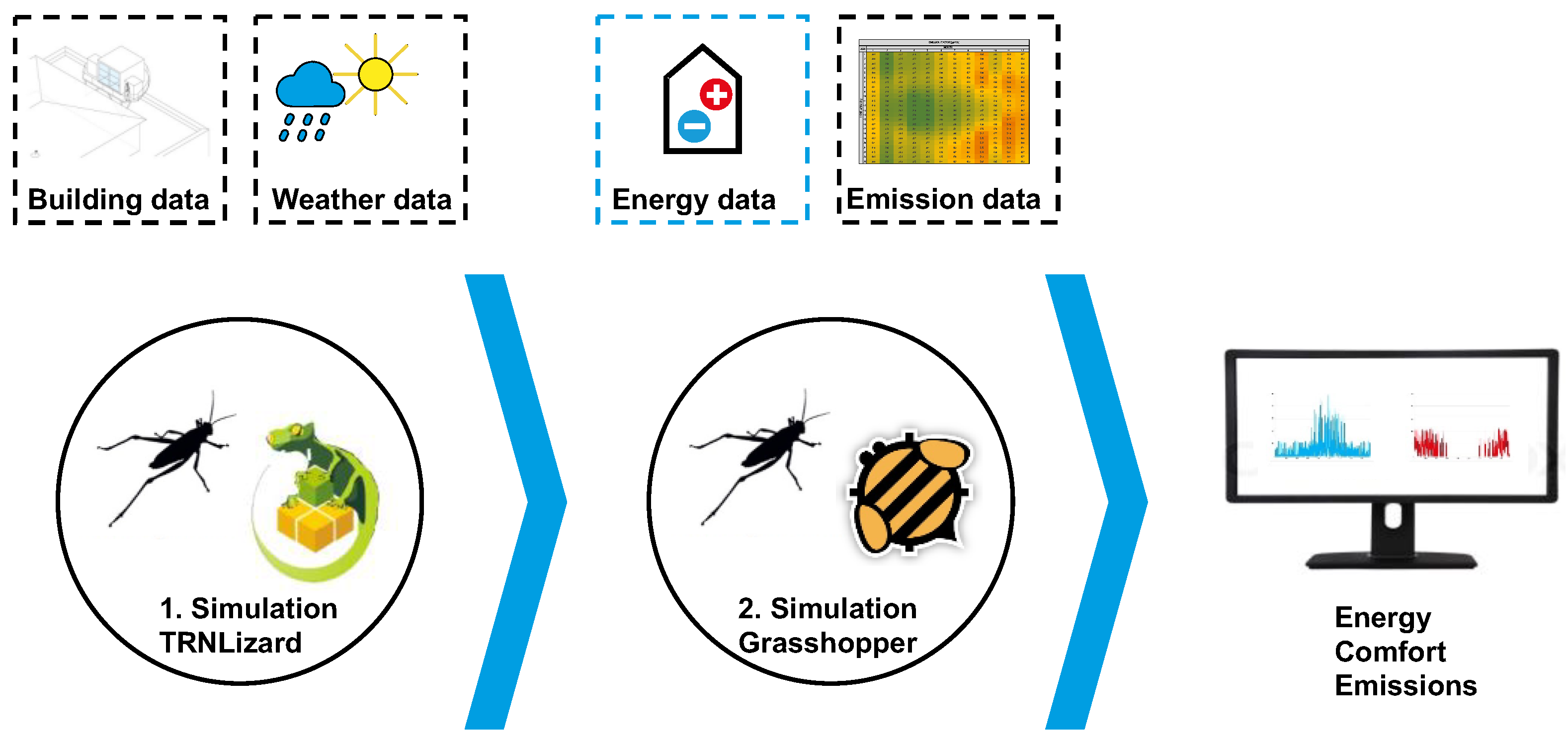
This paper uses three simulation software tools. The fundamental thermodynamic building simulation is performed in TRNLizard, representing the parametric version of TRNSYS 18 in the software environment of Rhino 3D [24,25]. TRNLizard is illustrated in the visual programming interface Grasshopper. Here, the building and weather data are implemented. HoneyBee [26], the second simulation software, performs the radiation simulation for the PV system. The third (static) simulation is performed in Grasshopper only. Here, the previously generated building energy data, radiation data, and the hourly emission data of the electrical grid evaluate the emission balance, focusing on the building operation.

Figure 1 displays the workflow of the thermal simulation. The first simulation step in TRNLizrad uses weather- and building-related data to generate annual energy and comfort data for the building. The weather predictive control uses the logarithmically mitted trend of local weather data. In the second step, a radiation analysis with HoneyBee is performed. Combined with the previously generated building energy data and the annual emission factor, these data evaluate the impact on emission performance using the Grasshopper software tool. Here, the previously outlined CO₂ predictive control can be applied, focusing on the 24 h minima of CO₂ emissions. In general, this paper uses thermal comfort, energy demand, and emission balance as evaluation parameters.

2.1.1. Base Case Model

The basic building model represents an in situ test facility, the Solarstation, a 23° southwest-oriented office room located on a rooftop in the urban environment of Munich. The room has a length of 4.30 m, a width of 4.30 m, a height of 3.30 m, and a large glass façade with a window-to-wall ratio of 90%. Venetian blinds, manually and automatically operable windows, and TABS represent the building technology. This covers a shading, ventilation, heating, and cooling system. The thermal characteristics of the building constructions are as follows: roof U-value 0.222 W/(m²K), external wall U-value 0.175 W/(m²K), floor U-value 0.266 W/(m²K), internal wall U-value 0.437 W/(m²K), window U-value 0.68 W/(m²K), thermal bridges 0.1 W/(m²K), and infiltration air change rate 0.2 1/h. In a previous study, the digital, thermodynamic model was validated with local weather and building measurement data, following the criteria of the ASHRAE guideline 14:2002 [14,27]. The validation can be confirmed using the normalized mean bias error, the coefficient of variation of the root mean square error, and the coefficient of determination for four type weeks.

The building system model displays the thermal and electrical storage in combination with a photovoltaic system. In general, the electrical power of the PV system is used to charge the storage. In that case, in practice, the thermal storage uses a heat pump to charge up. The discharging capacity is equivalent to the simulated energy demand of the building simulation without transportation losses (e.g., cables or ducts). The details of the system configuration and the prioritization of energy usage are outlined in detail in a previous paper [3].

The control strategy of the building technology has two modes: with and without predictive control (WEPC On/Off). In the predictive mode, the control strategy consists of two parts. The weather predictive control uses a 24 h logarithmically mitted trend of the future ambient temperature and solar radiation. This means that time steps closer to the present are weighted higher, but all 24 time steps have an impact. The control parameters of sun shading, ventilation, heating, and cooling systems are adapted compared to a standard control strategy. The detailed equations of the concepts about weather predictive control are outlined in a previous paper [15]. The second part of the predictive mode addresses the energy supply when filling the storage. Therefore, the minima of the next 24 h time steps of the emissions are identified in every time step to create a five-hour period to load up the storage system. The following parameters are adapted to the building model: storage capacity, rated charging capacity, unloading capacity, control strategy for charging, limit temperature for charging, storage losses, and storage efficiency. The standard loading strategy instead comprises a constant period to set the storage from 10 a.m. to 4 p.m. to use the PV energy production during the daytime.

2.1.2. Simulation Variants

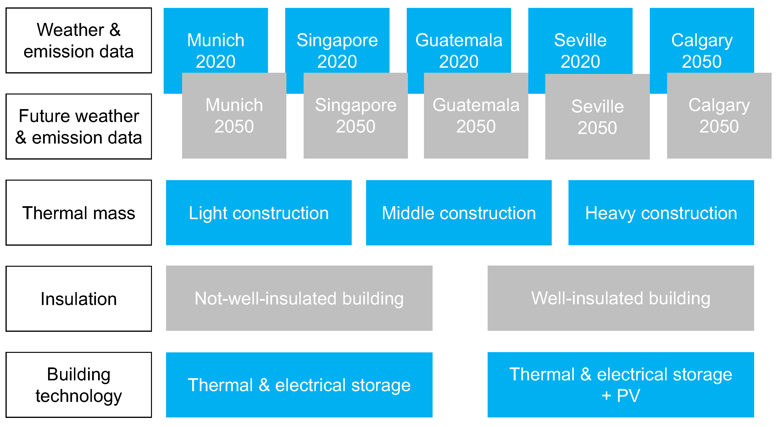
This paper uses a parametric study to answer the initially stated research questions and the hypothesis. The simulation is performed various times with slight changes in the assumptions to identify the impact. These changes are divided into simulation variant categories.

The first simulation variant category focuses on the impact of the climate location. Thereby, five different locations in different climate zones according to Köppen–Geiger are chosen, representing a moderate, tropical, subtropical, dry, and cold climate. This simulation variant category not only varies the climate location but also compares the concept’s impact on different levels of the electricity grid system, as the locations, by nature, are connected to their countries’ national electricity grid.

One of the primary outcomes of both previous studies was that the intelligent control strategies’ energy and CO₂-saving potentials could be much higher with poorly insulated buildings. This forms the second simulation variant category. Hence, the U-values of the measurement room, which fulfill the thermal requirements of the German building code [28], are increased for the external wall from 0.22 to 1.0 (W/m²K) and the window from 0.7 to 1.7 (W/m²K). These buildings could have more saving potential and represent the not-refurbished, primary building stock worldwide, not only in Western countries like Germany.

As mentioned in both previous studies, the third simulation category, thermal mass, considerably impacts Munich’s energy and CO₂ performance. Again, this paper analyzes the effect of light, middle, and heavy constructions. According to Din 4108-2, thermal mass quality is evaluated with the specific heat capacity Cw/A. These are the categories as follows: heavy: (Cw/A > 130 (K m²)), middle (Cw/A between 130 (K m²) and 50 (K m²)), and light (Cw/A > 50 (K m²)) [29]. This is especially interesting in combination with well- and not-well-insulated buildings, as it analyses the effect of traditional and non-traditional building styles in the various climate locations.

As emission and energy storage are two of the main objectives of this concept, the fourth category focuses on building technology. One simulation represents a thermal and electrical storage building system and an ideal heat pump. The second variant adds a photovoltaic system, enlarging the concept. The building technology is sized according to the previous studies. The thermal storage has a capacity of 2.52 kWh and a loading power of 0.37 kW, while the electrical storage comprises a capacity of 0.9 kWh and holds 0.25 kW loading power. The office is connected to a 1 m² PV area, and the COP for the air-to-air heat pump for heating is 5.24, while the COP for cooling accounts for 4.0, representing a ground-floor system. This analysis can help to understand the impact of a building as an energy or potential CO₂ storage.

The last variant category focuses on the outlook and future behavior of the built world. Thereby, weather data for the year 2050 following the IPCC scenario RCP 8.5 are assumed to estimate the impact of the predictive control strategy [30]. In addition, the emission factor is lowered in all locations by 50%. While this assumption is rather simple and will only give a small insight into future behavior, predicting future emission factors depends on many factors, e.g., politics, society, funding for regenerative energies, and local conditions, to extend the regenerative powers. These factors are highly unpredictable. Developing a more precise prediction method for the emission factor is beyond the scope of this paper. Figure 2 illustrates an overview of the simulation variant categories that result in 240 simulation variants.

2.2. Weather Data and Emission Data

The following subsections outline the weather and emission data of the five climate locations. To generate an overall, worldwide impression of the impact of the energy- and emission-saving potential of the control strategy, the first criterion in the sections of the location is the climate category according to Köppen–Geiger: Munich, Germany (moderate—Cfb), Singapore City, Singapore (tropical—Af), Guatemala City, Guatemala (subtropical—Cwa), Sevilla, Spain (hot/dry summer—Csa), and Calgary, Canada (cold—Dfc). At the same time, each location is connected to its national electricity grid, with a different dynamic composition and behavior regarding emissions, mainly based on the share of integrated regenerative energies.

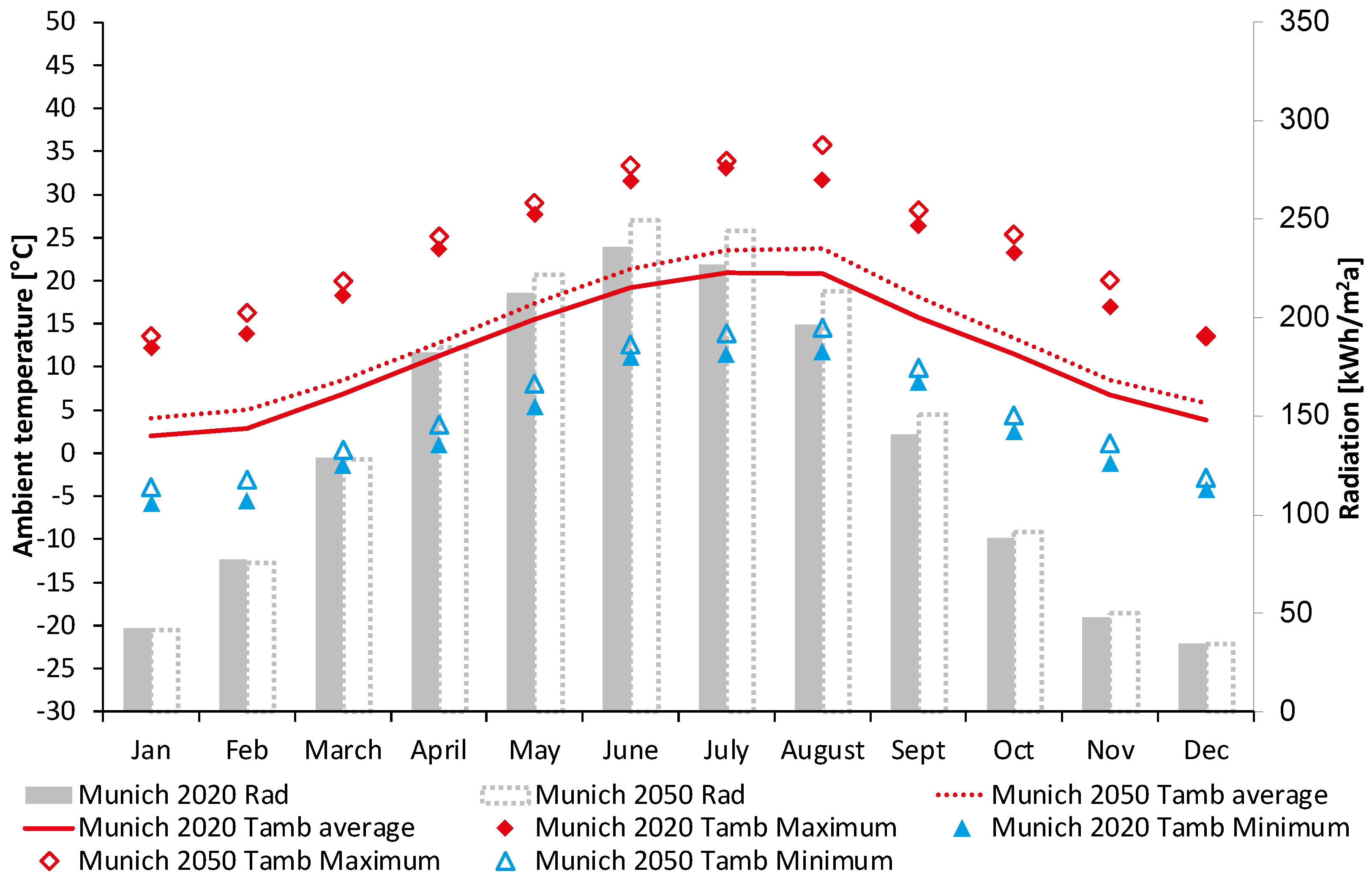
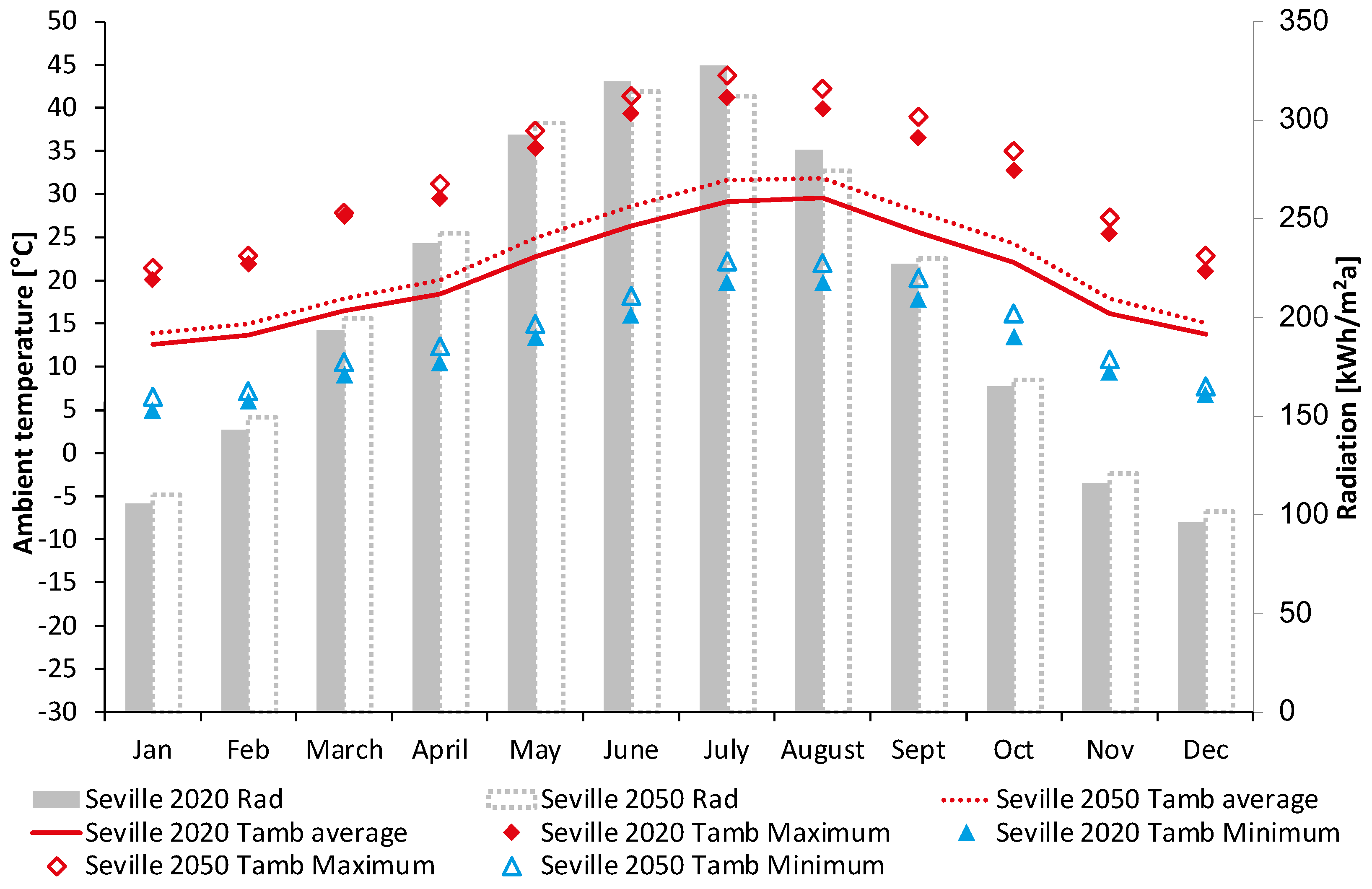
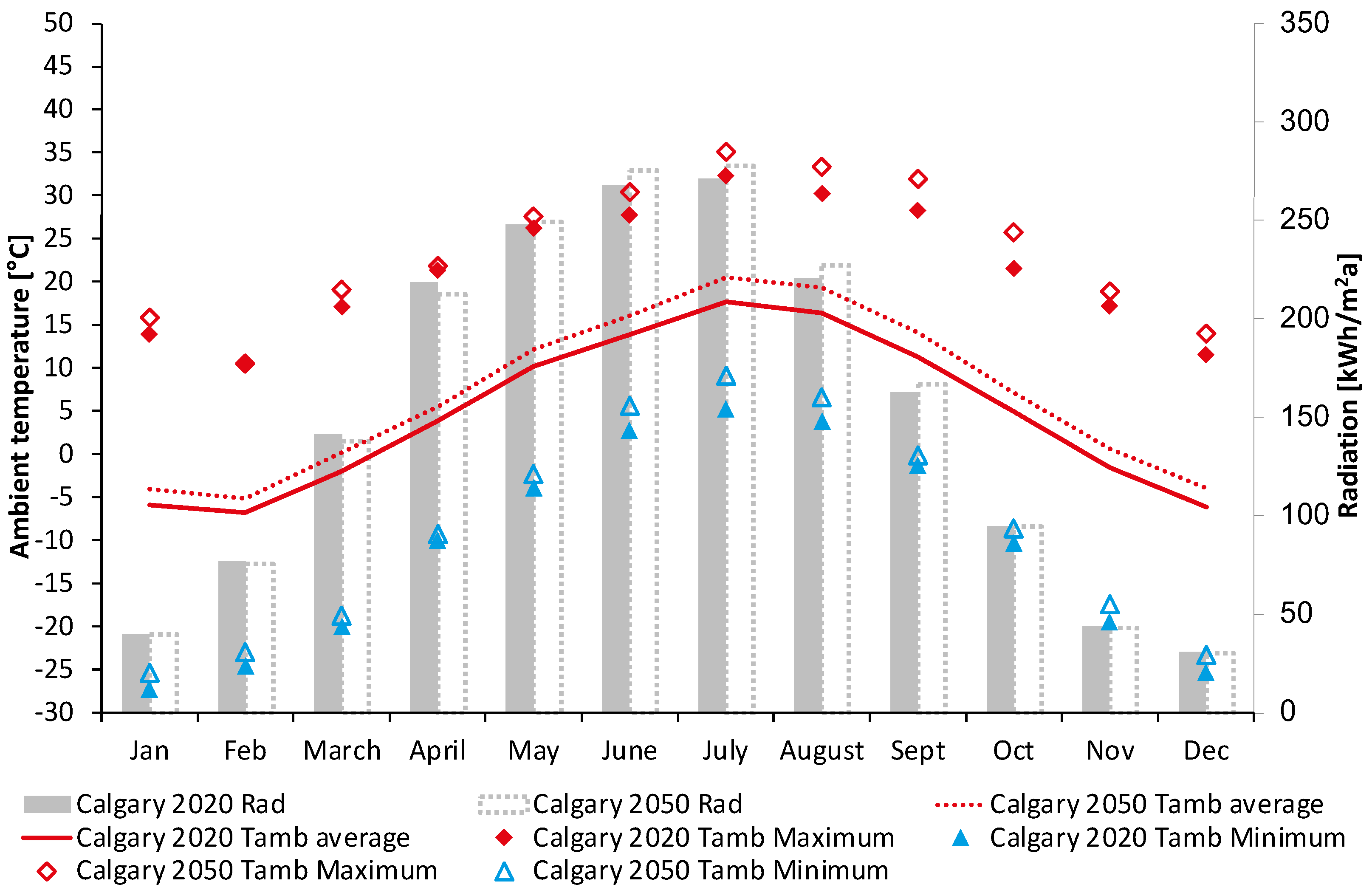
Two types of graphs are used to analyze the individual climate locations. The first focuses on the weather data, displaying the temperature and radiation. The minimum and maximum temperature of the month and the dynamic annual dry bulb temperature are outlined in °C, linked to the left y-axis. The right axis displays the monthly radiation in kWh/m². Solid lines show the weather data for 2020, whereas dashed lines represent the future weather data for 2050. The weather data found in each location’s typical meteorological year (TMY) data set is interpolated for 2050 using the IPCC RCP 8.5 scenario [30,31]. The thresholds for the axis are identical for all climates to maintain comparability, even though it sometimes reduces the readability of the graphs.

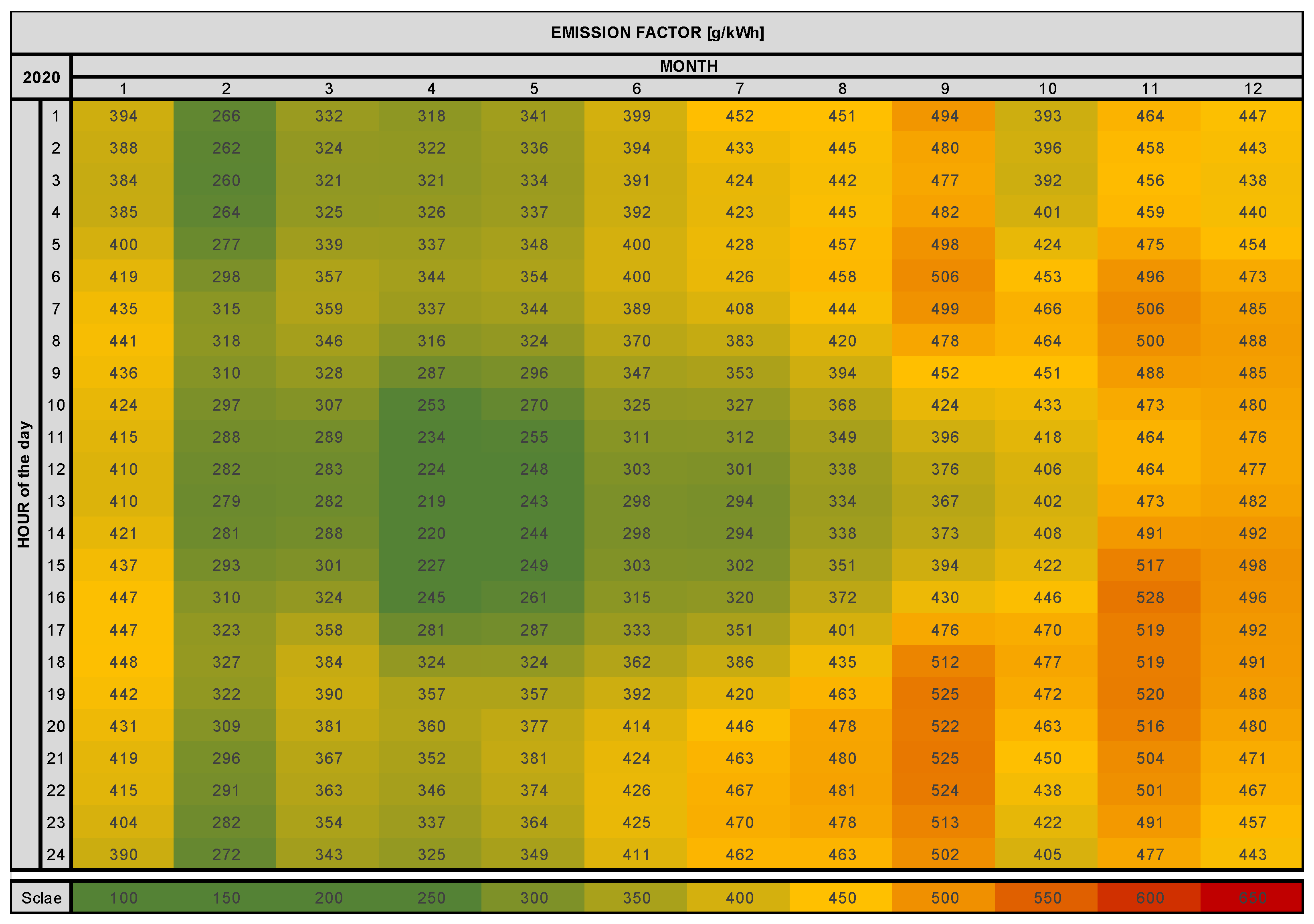
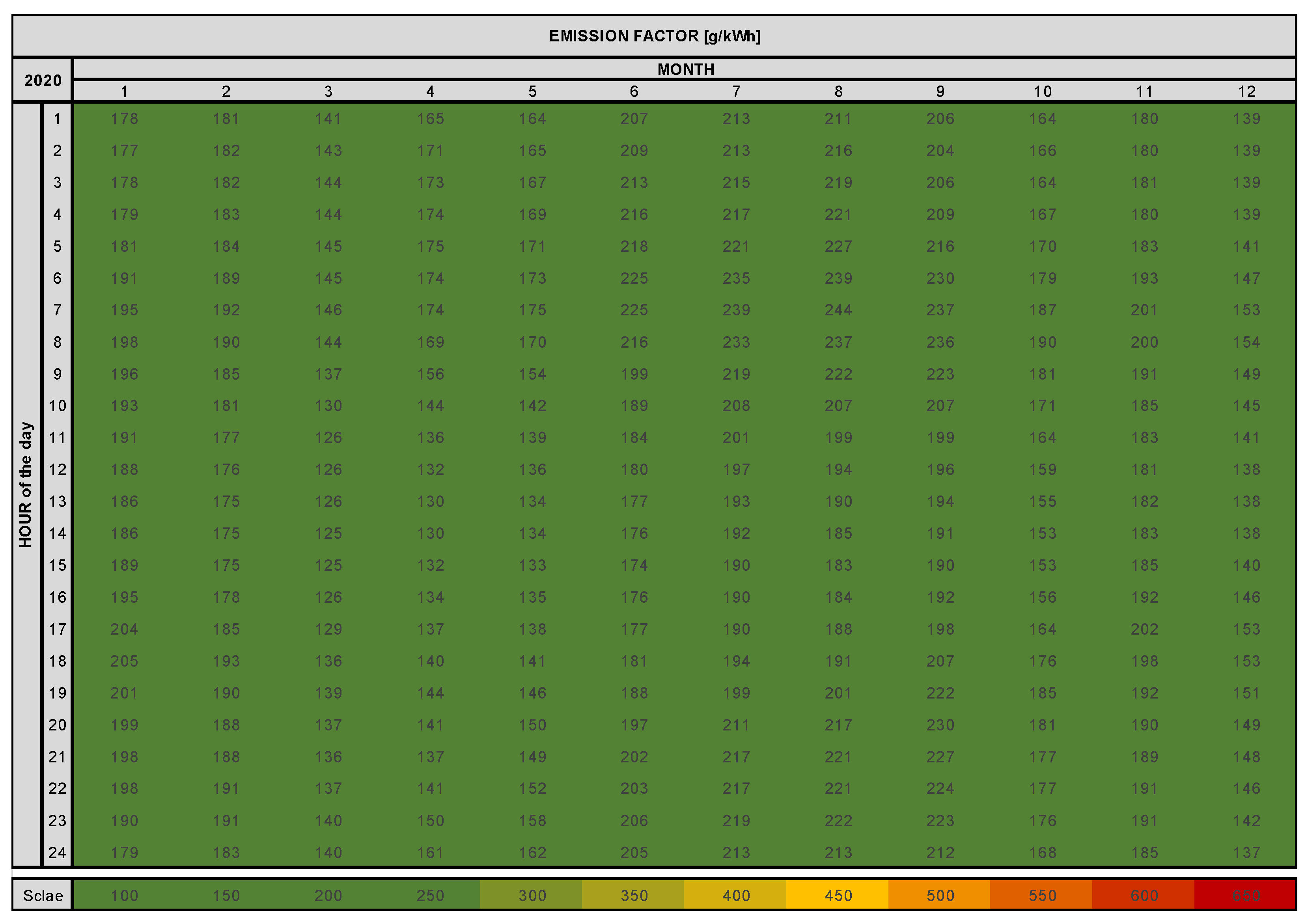
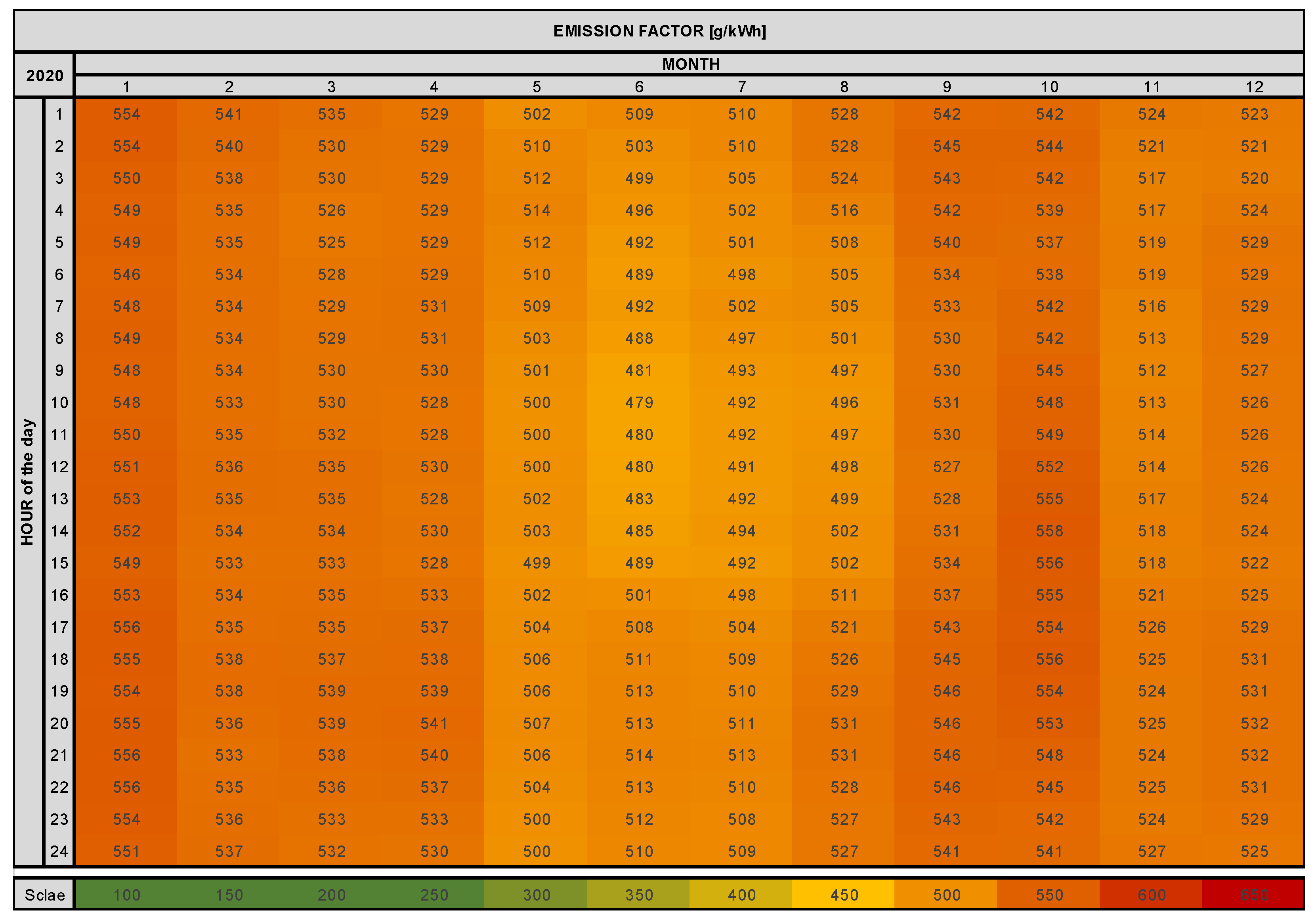
The second figure outlines the annual dynamic emission data of the location. The carpet plot follows the daily 24 h on the y-axis, while on the x-axis, the months of the year are listed. This forms an overview of the hourly emission factor averaged each month, with high emission values in red and low values in green. The data use the production capacity, level of consumption, electricity import and export, and the electricity price of the power grid to calculate an hourly emission value [32]. The thresholds of the color scale are kept constant for all five locations to maintain comparability, even though it reduces the data quality for each site.

2.2.1. Moderate Climate—Munich

Munich is in southern Germany and has a humid continental climate with cold winters and mild summers (Köppen–Geiger: Cfb). In 2020, the city had an average ambient temperature (Tamb) of 10.4 °C, with maximum temperatures reaching 36.5 °C and minimum temperatures dropping to −7.6 °C (Figure 3) [33]. The primary solar radiation hits in the summer, but in the spring and fall seasons, solar radiation can cause overheating. Heating systems are standard, while cooling units, for the most part, are only used in formal offices.

Figure 4 illustrates the overall annual CO₂ emissions [32]. During the day, emissions are generally lower based on photovoltaics, especially in summer. In the cold periods, including spring, emissions are lower all across the day, as wind energy dominates the emission value. The overall average value of 392 g/kWh is still relatively high and leaves room for improvement.

Looking ahead to 2050, climate models predict Munich will experience an overall warming trend, with average temperatures increasing by 2–3 °C [34]. This increase in temperature is likely to be accompanied by more frequent and intense heat waves, as well as an increase in the frequency and severity of extreme weather events such as heavy rainfall and flooding. Based on the urban heat island effect, these numbers could even be exceeded in a city like Munich [35]. However, several measures could be taken to mitigate the impacts, including implementing green roofs, creating urban parks and green spaces, and installing water areas. As Germany is part of the EU and committed to climate neutrality, a significant increase in renewable energies and lower emissions all across the year can be expected.

2.2.2. Tropical Climate—Singapore

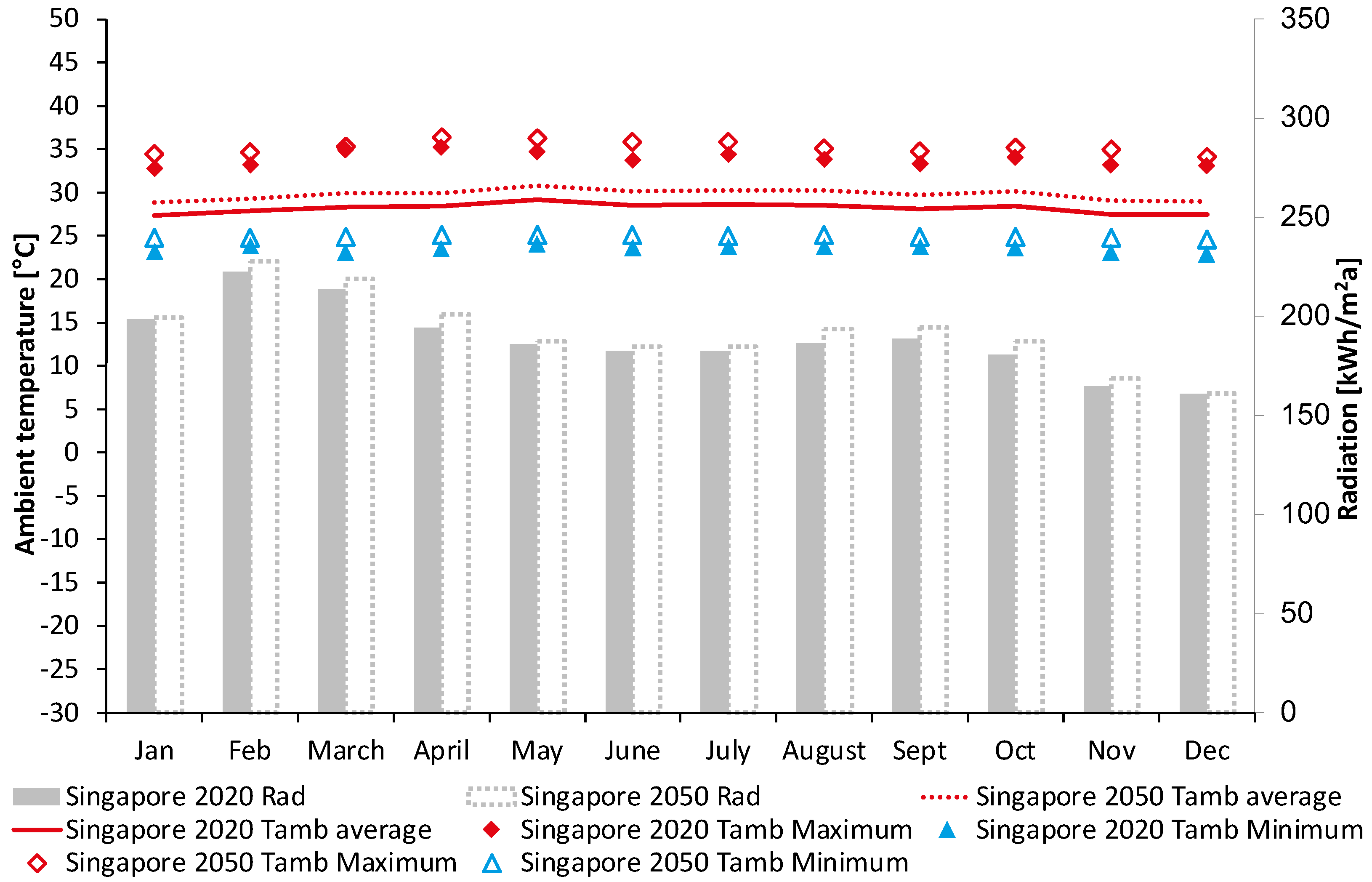
In 2020, Singapore experienced warm and humid weather conditions throughout the year, categorized by Af by Köppen–Geiger. Figure 5 shows that Singapore’s ambient temperature remains consistent, with average highs from 29 to 33 °C and lows from 23 to 27 °C, with heavy rainfalls in the rainy season. The city-state is near the equator, resulting in a tropical climate with minimal seasonal variations, as illustrated in Figure 5. However, the humidity levels often make the perceived temperature feel higher than the actual readings. Singapore also receives significant solar radiation throughout the year due to its proximity to the equator. The city experiences around 1900 to 2200 h of sunshine annually [36].

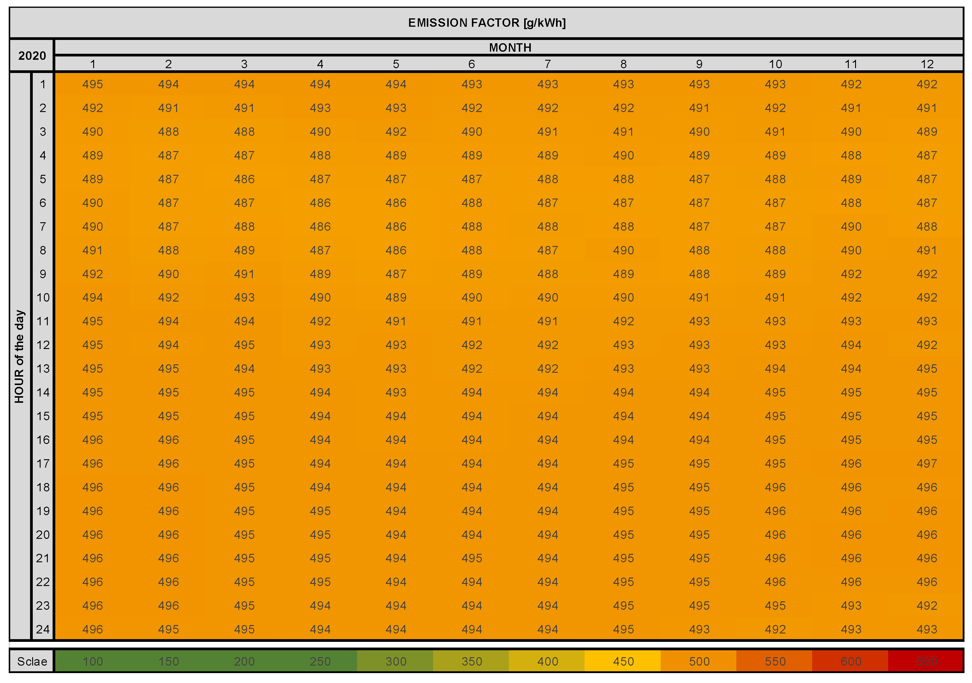
As a small, densely populated city-state with limited land resources, Singapore heavily relies on imported energy sources, mainly natural gas, to generate electricity. Natural gas is a cleaner fossil fuel than coal and oil, resulting in lower but nearly constant yearly emissions, as shown in Figure 6. But, of course, the state needs to use its very high potential for regenerative energies in the future, as high solar radiation is present all year long.

Climate change in Singapore is having a significant effect on both the environment and architecture of the city. Elevated temperatures and increased rainfall patterns are already being observed in Singapore, which could lead to increased air pollution, rising seas, and compromised biodiversity in the region [37]. Furthermore, changes in the climate, from extended rainfall periods to more extreme and frequent storms, present the city many challenges in adapting building styles to withstand climatic conditions [38]. In order to remain sustainable, Singapore has to gradually adapt its urban infrastructure to become more climate resilient [39]. Therefore, regenerative energies could play a significant role. Solar radiation is very high, and there are several potentials for hydropower. The government has set ambitious goals and outlined strategies to integrate renewable or regenerative energies into its energy mix, such as the 2030 Green Plan or the SolarNova Program, with the aim to have 2 GWp by 2030.

2.2.3. Subtropcial Climate—Guatemala

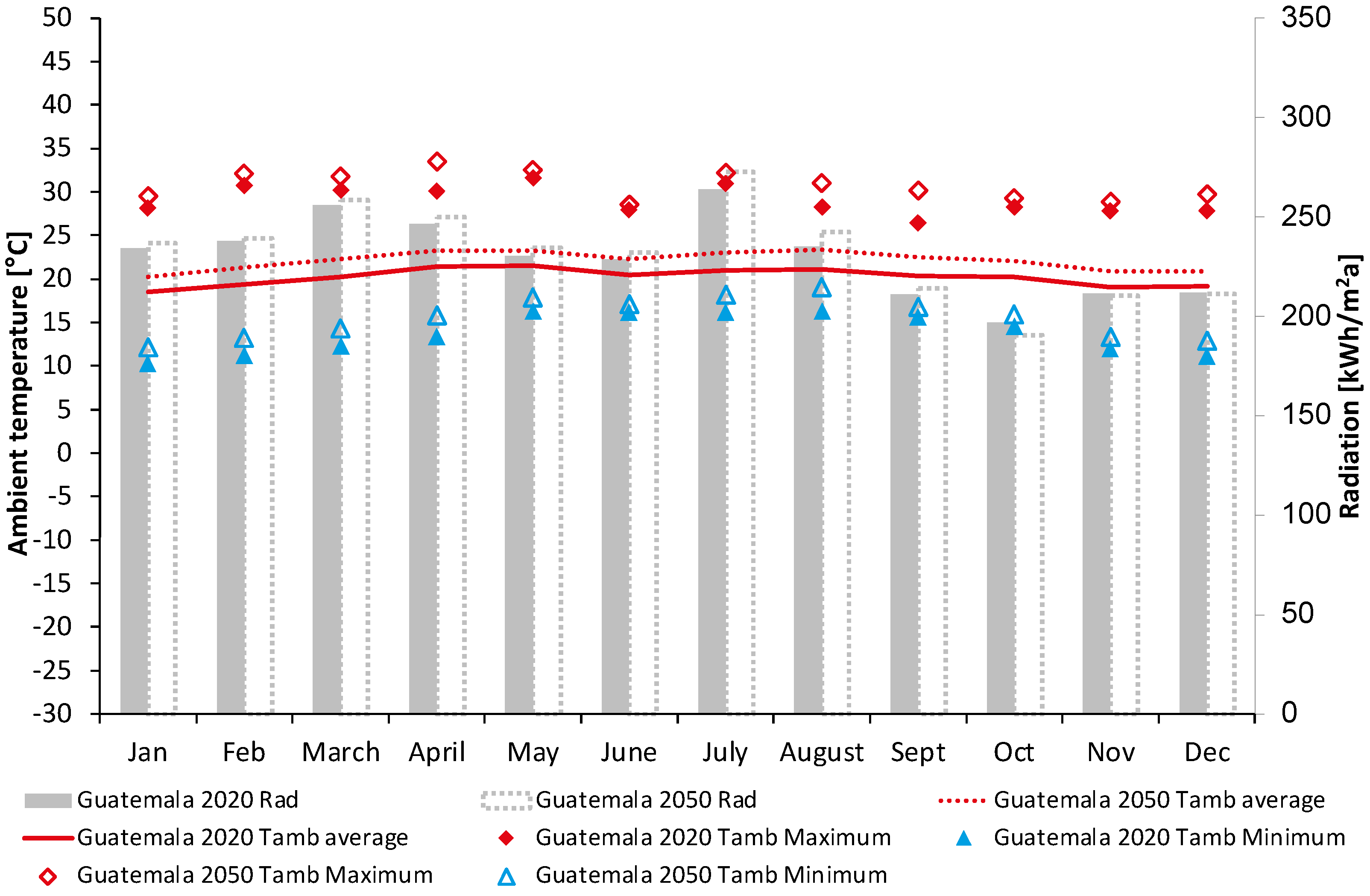
The capital of Guatemala (Köppen–Geiger: Cwa) is situated in a valley at an elevation of approximately 1500 m above sea level. The ambient temperature in Guatemala City remains relatively stable throughout the year, with average highs ranging from 25 to 28 °C and average lows ranging from 13 to 16 °C, as displayed in Figure 7. Due to its altitude, the city enjoys a temperate climate characterized by mild temperatures, especially in the evenings and early mornings. The rainy season, from May to October, brings occasional heavy downpours, while the dry season, from November to April, experiences sunny days with limited rainfall. In terms of solar radiation, Guatemala City benefits from abundant sunlight. Being close to the equator, the city experiences a consistent day length throughout the year, resulting in substantial solar exposure and, therefore, allowing ample opportunities for solar energy utilization and solar power generation.

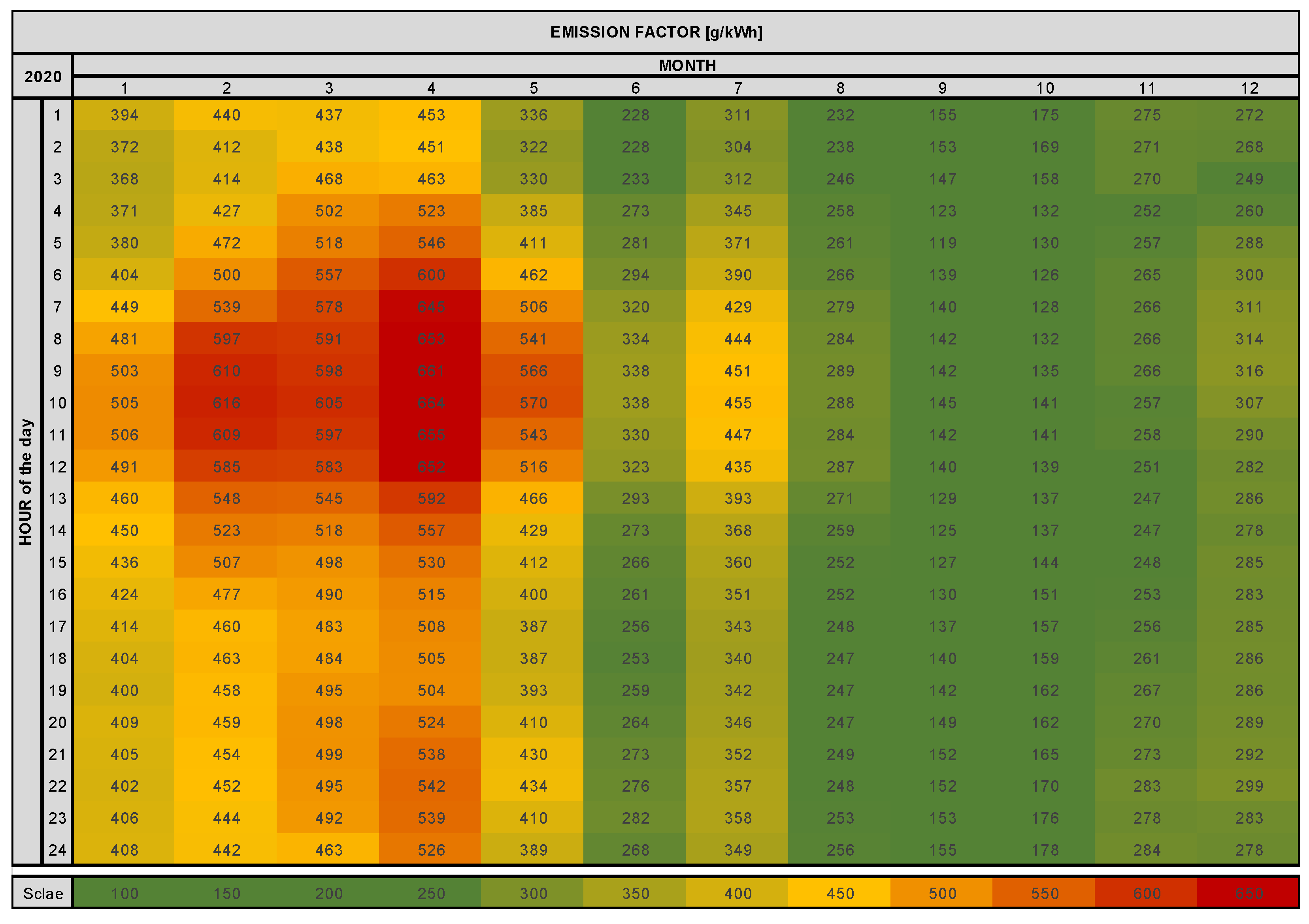
The electricity grid in Guatemala is a complex system that plays a significant role in meeting the country’s energy needs. Guatemala’s electricity generation primarily relies on renewable and non-renewable energy sources. As Figure 8 outlines, the emission factor in Guatemala’s electricity grid is relatively low compared to many other countries. Hydropower is Guatemala’s dominant renewable energy source, accounting for a substantial portion of electricity production. However, Guatemala has significant potential for expanding its use of renewable energies beyond hydropower. The country has untapped resources for solar energy and wind power. It is essential to note that Guatemala also relies on fossil fuels such as oil and coal for electricity generation.

Predicting the exact weather conditions in Guatemala City in 2050 is challenging, but climate projections suggest increasing ambient temperatures. According to the Guatemalan National Institute of Seismology, Volcanology, Meteorology, and Hydrology [40], temperatures are expected to rise due to global climate change. This could lead to more frequent and intense heat waves, affecting public health, agriculture, and water resources, mainly due to the urban heat island effect and urbanization. Based on the already sufficient climate potential for regenerative energies, the future emission factor primarily depends on financial and political decisions. To promote renewable energy, Guatemala has implemented policies and incentives to encourage private investments in renewable energy projects [41]. Neighboring countries like Costa Rica have already proved that a complete regenerative energy grid is possible in that climate.

2.2.4. Hot Mediterranean Climate—Seville

Seville, a city in southern Spain, experiences a Mediterranean climate with dry, hot summers and mild winters (Köppen–Geiger: Csa). The ambient temperature in Seville during 2020 remained consistently high, especially in the summer months. Average highs ranged from 30 to 40 °C, with occasional heatwaves leading to even higher temperatures. As shown in Figure 9, winters are relatively mild, with average lows ranging from 4 to 8 °C. Like most of Spain, Seville benefits from solar radiation throughout the year. Rainfall is scarce during the summer, with occasional strong showers in the winter months. The relatively dry conditions and high solar radiation levels contributed to Seville’s reputation as one of Europe’s hottest cities [42].

The emission factor in the electricity grid of Spain is influenced by the energy sources used for power generation. Historically, the region has relied on fossil fuels, such as natural gas and coal, contributing to greenhouse gas emissions. However, there has been a growing emphasis on reducing emissions and transitioning to cleaner energy sources in recent years all over Spain. With its high mountains in the middle and the overall high solarization, hydropower, wind, and solar power generation are easily accessible in the area. The country has been actively transitioning to renewable energy sources, with a considerable share of over 50% of its electricity coming from wind, solar, and hydroelectric power [43]. As a result, Spain’s electricity grid already has a low annual emission value of 178 g/kWh compared to countries heavily reliant on coal-fired power plants, as shown in Figure 10.

Climate projections suggest a continuation of rising ambient temperatures in Seville. According to the Spanish Meteorological Agency, Seville is expected to experience an increase in average temperatures due to climate change and even less frequent but heavier rainfalls [42,44]. This could lead to more intense heat waves, with the summer climate transforming into desert-like scenarios. Spain is actively promoting the integration of regenerative energies into its electricity grid to combat climate change and enhance sustainability. Renewable energy sources such as hydropower, solar photovoltaic systems, wind farms, and biomass facilities are gaining traction. Solar power is abundant in Seville, making it an attractive option for clean energy production. Based on the Western standard and the holistic potentials in various regenerative energy sources, Spain has all the measures to follow the European roadmap of climate neutrality in 2050 [12].

2.2.5. Cold Climate—Calgary

As a city in a continental, cold climate (Köppen–Geiger: Dfc), Calgary’s weather is characterized by distinct seasons. Figure 11 presents that the ambient temperature in Calgary during 2020 varied significantly across the seasons. Winters were cold, with average highs ranging from −5 to −2 °C, while average lows dropped from −13 to −9 °C. Spring and fall brought milder temperatures, with average highs around 10 to 15 °C, and summers were warm, with average highs ranging from 20 to 25 °C. The weather in Calgary is also influenced by periodic weather systems, such as Chinook winds, which can lead to rapid temperature fluctuations in winter months. Solar radiation in Calgary sees considerable variation throughout the year. Summers experience long daylight hours, providing solar exposure, while winters have shorter daylight periods [45].

Alberta’s electricity grid has historically relied on fossil fuels, especially coal and natural gas. This dependence on fossil fuels leads to high greenhouse gas emissions. However, in recent years, the province of Alberta and the state of Canada have been making significant strides in incorporating regenerative energies into their electricity grid, e.g., with the International Airport of Calgary founding on a geothermal heat pump [46]. Renewable energy sources, such as wind, solar, and hydroelectric power, have been integrated into the grid but still comprise a small share. The city’s solar potential is moderate compared to more sun-exposed regions, but solar energy remains a viable option for electricity generation and other applications. This results in an annual high emission value with an average of 525 g/kWh, as shown in Figure 12.

Climate projections suggest an increase in ambient temperatures. According to the Government of Canada’s Climate Atlas, Calgary is expected to experience warmer temperatures due to ongoing climate change [45]. By 2050, average temperatures may rise by several degrees Celsius, leading to more frequent summer heat. These warmer conditions could impact various sectors, including agriculture, water resources, and public health, and increase the potential of solar radiation. Incentives and policies have been put in place to support the growth of regenerative energies. The transition to regenerative powers in Canada’s electricity grid aligns with global efforts to combat climate change and promote more sustainable energy. As renewable energy technology advances, Alberta is poised to expand its clean energy capacity further and reduce its reliance on fossil fuels in the coming years [47]. One big advantage of Canada is the ratio between population and land area. Furthermore, Alberta has abundant renewable energy potential, including wind and hydroelectric power. Considering these potentials, in combination with the wealth of the state, under the right political circumstances, the energy transition for Canada can be performed straightforwardly.

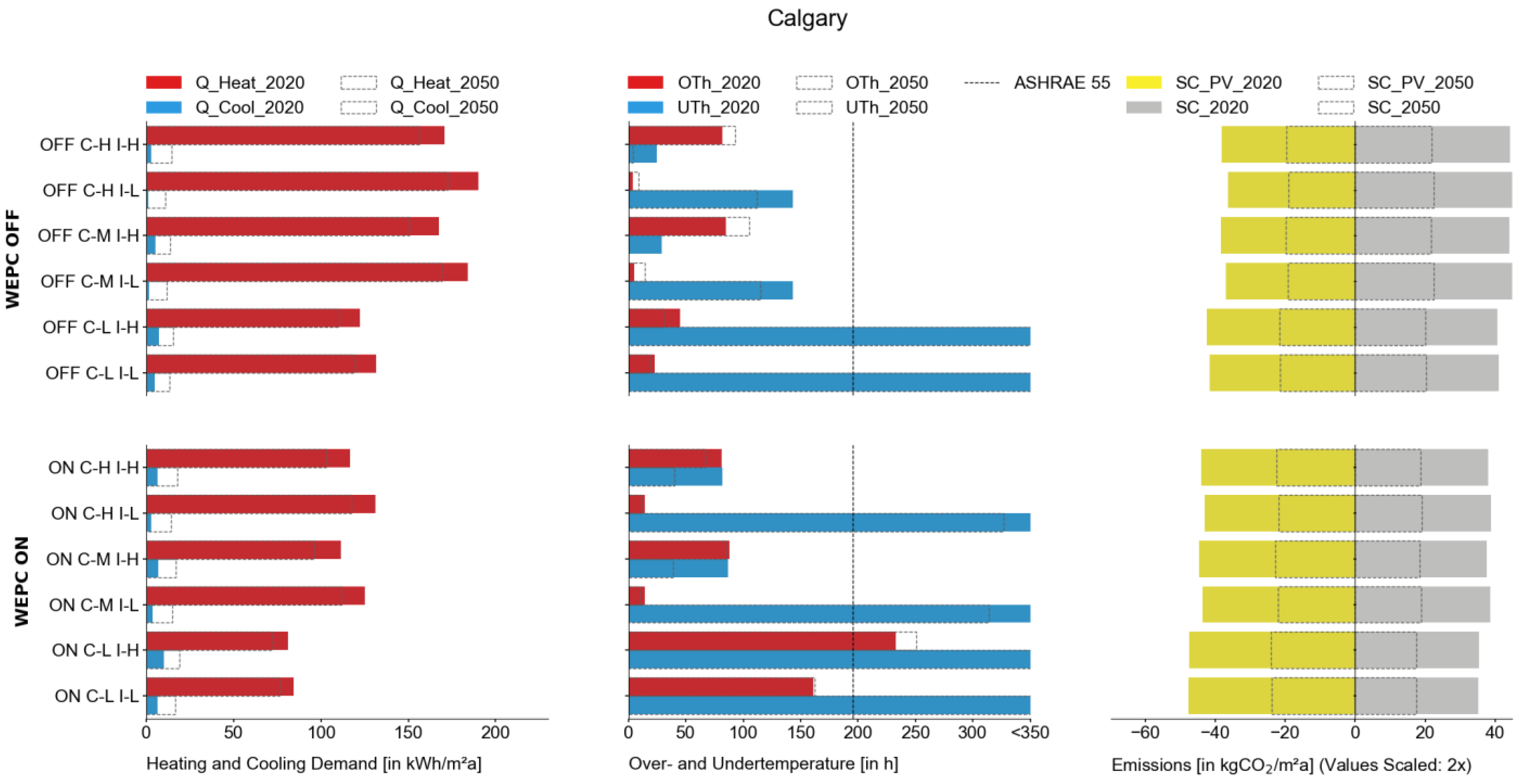
3. Results and Evaluation

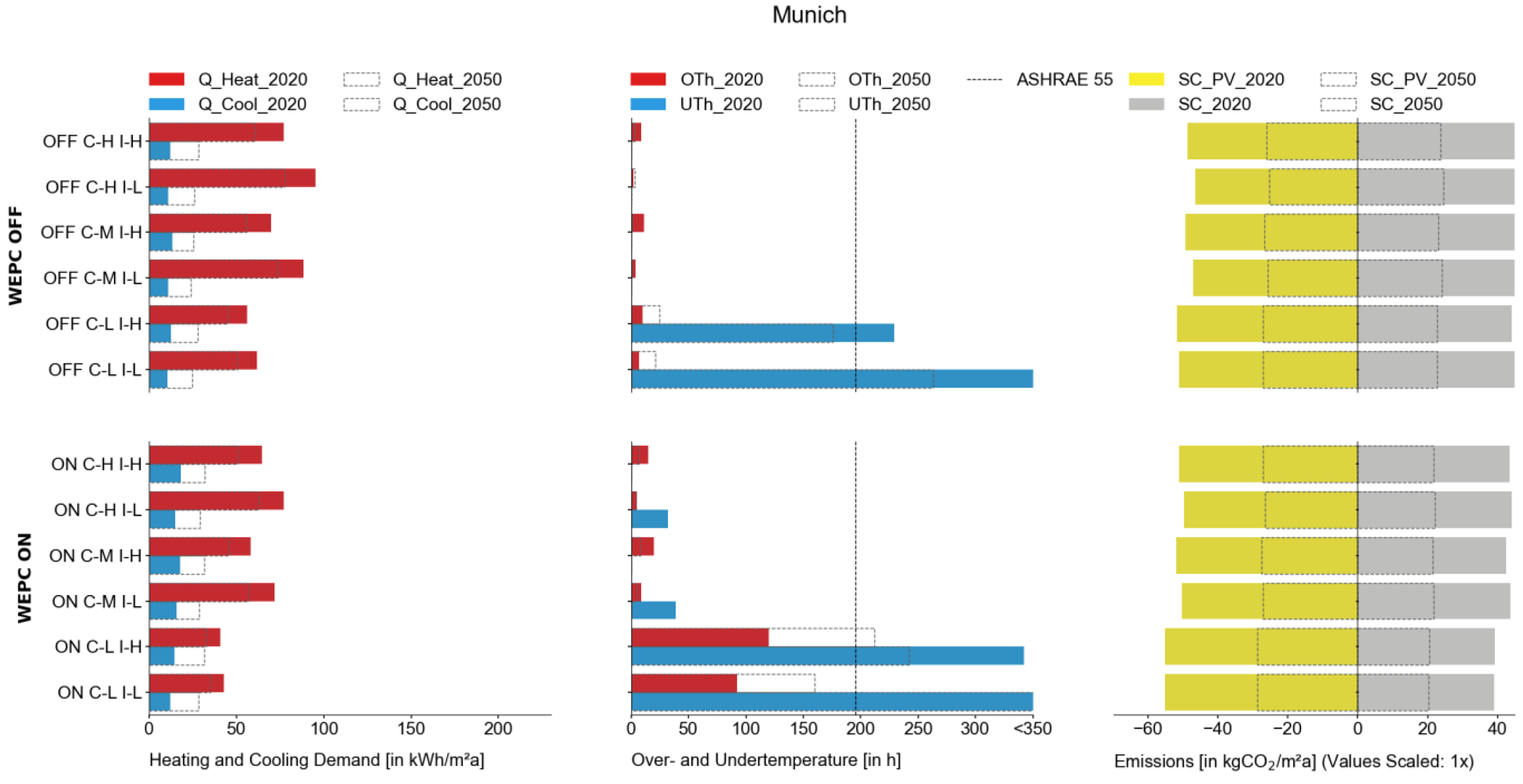
Following the fundamental data structure, this section outlines the thermodynamic simulation results for each climate location. Three graphs per location illustrate the three evaluation categories for the previously outlined simulation variants for 2020: energy demand, thermal comfort, and emission balance. The energy demand on the left shows the annual heating and cooling demand in kWh/(m²a) (Q_heat, Q_cool). The thermal comfort in the middle graph analyzes the over- and undertemperaturehours according to ASHRAE 55 2004 (OTh; UTh) [48]. The graph on the right shows the emission performance in kgCO₂/m². Please pay attention to the scaling factor for the emissions. In each variant section, the dashed line presents the future scenario using the weather and emission data for 2050, while the full color illustrates the simulation variants for 2020. The simulation variant abbreviations are as follows: On/Off—weather predictive control or standard control; C-L, C-M, C-H—construction light, middle, or heavy; I-L, I-H—insulation light or heavy; and SC, SC_PV—system configuration with thermal storage or with thermal and electrical storage and PV. With these simulation results, the previously mentioned research questions are evaluated for each climate location. The first paragraph of each section addresses the general findings of the simulation results, followed by the influence of the thermal mass, insulation, and storage capacity in the second paragraph. The last paragraph features the overall functionality of the WEPC and gives an outlook of 2050, using the future scenario. Lastly, it is to be noted that simulation variants are only considered to perform well when fulfilling the thermal comfort requirements.

3.1. Moderate Climate—Munich

The heating demand in all simulation variants in Munich varies between 40 and 100 kWh/(m²a), and the cooling demand is significantly lower from 10 to 30 kWh/(m²a). The highest heating demand is recognized with WEPC Off, which has a high thermal mass and low insulation, and it is performed lowest with WEPC On, which has a middle thermal mass and high insulation. The highest cooling demand is necessary for WEPC On, with a high thermal mass and insulation, and is lowest for WEPC Off, with a middle thermal mass and low insulation. In general, one can see that the light construction variants do not fulfill the thermal comfort requirements. The emissions in Munich are quite constant. The simulation variants with PV create energy savings in a range of −50 kgCO₂/(m²a), while without PV, the emissions vary around +40 kgCO₂/(m²a).

Tackling the impact of the WEPC, one can see in Figure 13 that with WEPC, the heating demand decreases drastically (up to 50%), while the cooling demand in absolute numbers only slightly increases. This is also true for the over- and undertemperaturehours for the middle and heavy construction variants that are below the threshold. Independent of the control strategy, it is clearly visible that the higher the insulation, the lower the heating demand. On top of that, it is also true that the lower the thermal mass, the lower the heating and cooling demand. The emissions only slightly vary for the individual simulation categories. The lighter the construction for ESC with PV, the more energy savings increase. Furthermore, it shows that for SC1 with PV, the emission savings are higher with thermal insulation. The simulation variants without a PV system show constant values for emission performance, except for the light simulation variants.

Overall, the WEPC works very well in Munich’s moderate climate. The heating demand, particularly for massive constructions, is improved significantly without harming thermal comfort. The cooling demand only increases slightly in absolute numbers and confirms the fact that cooling demand was not generally necessary in Munich in 2020. The future scenarios show a small decrease in heating and a significant decrease in cooling demand, particularly for heavy constructions. But, again, the simulation variants with WEPC reduce the increase compared to those without WEPC. The emissions decrease overall with the future scenario in 2050 by up to 50%. The SC only with storage systems reduces with and without WEPC by 50%. In contrast, the emission savings for the simulation variants with PV only decrease by 45%, as the photovoltaic system still improves the emission performance and solar radiation changes slightly in 2050.

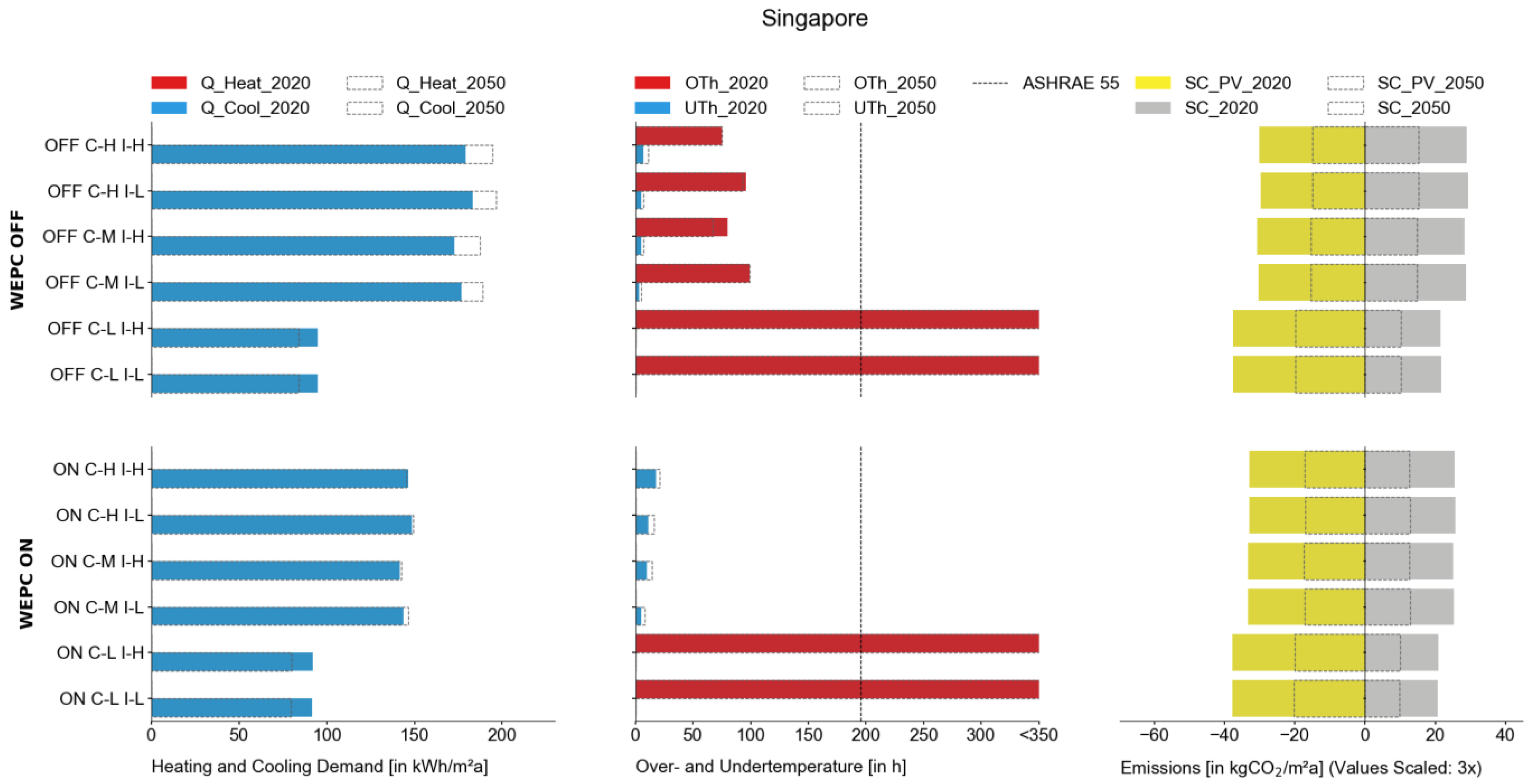
3.2. Tropical Climate—Singapore

In the tropical climate of Singapore, no heating energy is needed, while cooling dominates the energy balance with 80 to 200 kWh/(m²a) for the individual simulation variants. This very high cooling demand indicates that thermal comfort can be provided for the middle and heavy construction variants. In contrast, the light simulation variants cannot stay below the threshold in all cases. In some rare moments, UThs exist that can be linked to an overcooling of the building by the powerful cooling system. Considering the scaling factor, the emissions for SC are in a range of up to +80 kgCO₂/(m²a). For the simulation variants with PV, the saving reaches values up to −110 kgCO₂/(m²a).

The increase in thermal mass leads to a decrease in the cooling energy demand and does not have a big effect on the OThs. Higher thermal insulation slightly increases the cooling energy. Thermal mass only slightly decreases the emission savings with PV around 2–4 kgCO₂/(m²a), while thermal mass and insulation do not have a noticeable impact. Overall, the emission balances for the simulation categories stay on a similar level that can be linked to the constantly high level of emissions in Singapore’s electricity grid all day and year.

Figure 14 illustrates all WEPC variants that have cooling demands up to 40 kWh/(m²a) lower than with a standard control. In addition to that, the results show that the WEPC variants have no OThs anymore. The small increase in the UThs is a small sign of over-cooling in the morning hours when WEPC anticipates office users. For the standard control, the future cooling demand in 2050 rises with ~10 kWh/(m²a), whereby with the WEPC, the cooling demand nearly stays at the same level. Overall, simulation variants with WEPC have around 10 kgCO₂/(m²a) fewer emissions with SC and the same amount of emission savings with PV. The future variants show that the emission savings for SC_PV are reduced by 50%, while the system configurations without PV show a decrease until 2050 of around 55% on average.

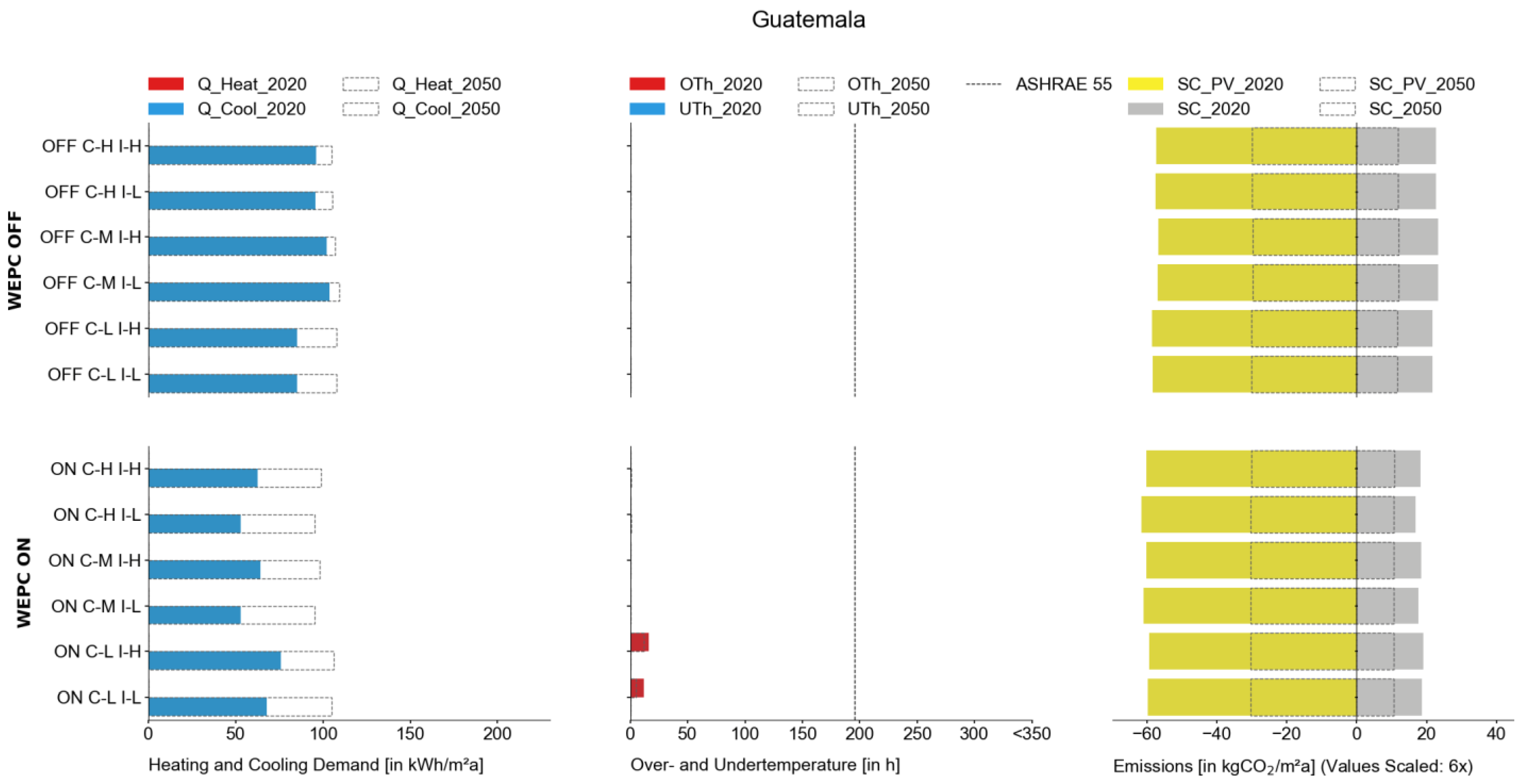
3.3. Subtropical Climate—Guatemala City

The very pleasant and constant temperature of subtropical Guatemala City leads to no heating demand and no OThs and UThs. Further, it is a location where light construction variants can fulfill the thermal comfort conditions. The cooling energy demand varies between 50 and 100 kWh/(m²a). The lowest cooling demand, 52 kWh/(m²a), occurs for a simulation variant with WEPC On, middle–heavy construction, and with low thermal insulation. The emission savings with PV stay consistently at a very high level of −340 kgCO₂/(m²a), which can be linked to the constantly high solar yields in the diurnal climate of Guatemala. In contrast, the emission performances without using solar electrical energy vary on medium–high between +100 and +120 kgCO₂/(m²a) for the year 2020, considering the scaling factor of 6. The previously described low emission values for Guatemala’s electricity grid are responsible for this good performance.

In a subtropical climate, the effect of thermal mass is not consistently visible in the considered simulation variants. For the standard control, there is no trend noticeable for the thermal mass, but more thermal insulation for the middle and light variants leads to a small increase in cooling energy. In the cases of WEPC being active, more thermal mass leads to a lower cooling energy demand. Furthermore, the cooling energy demand decreases by 10–15% with less thermal insulation for the predictive control. With WEPC active, the emission savings for SC_PV increase from −340 to up to −360 kgCO₂/(m²a), as well as the emission performances for SC decrease from +120 to the lowest of +100 kgCO₂/(m²a) for the light construction variant.

Figure 15 shows that simulation variants with WEPC generally perform better with up to 50% less cooling energy than their standard control equivalents. This especially works well for simulation variants with high thermal mass. In 2050, the cooling energy demand will increase for all variants, especially for the WEPC active with up to 30 kWh/(m²a), but there are still no noticeable OThs. For SC, the emissions with WEPC decrease by 20%, and the emission savings with PV increased by up to 25 kgCO₂/(m²a). This proves the impact of predictive control in 2020. In 2050, both SC and SC_PV will be reduced to 50%, connected to the lower emission values of the electricity grid.

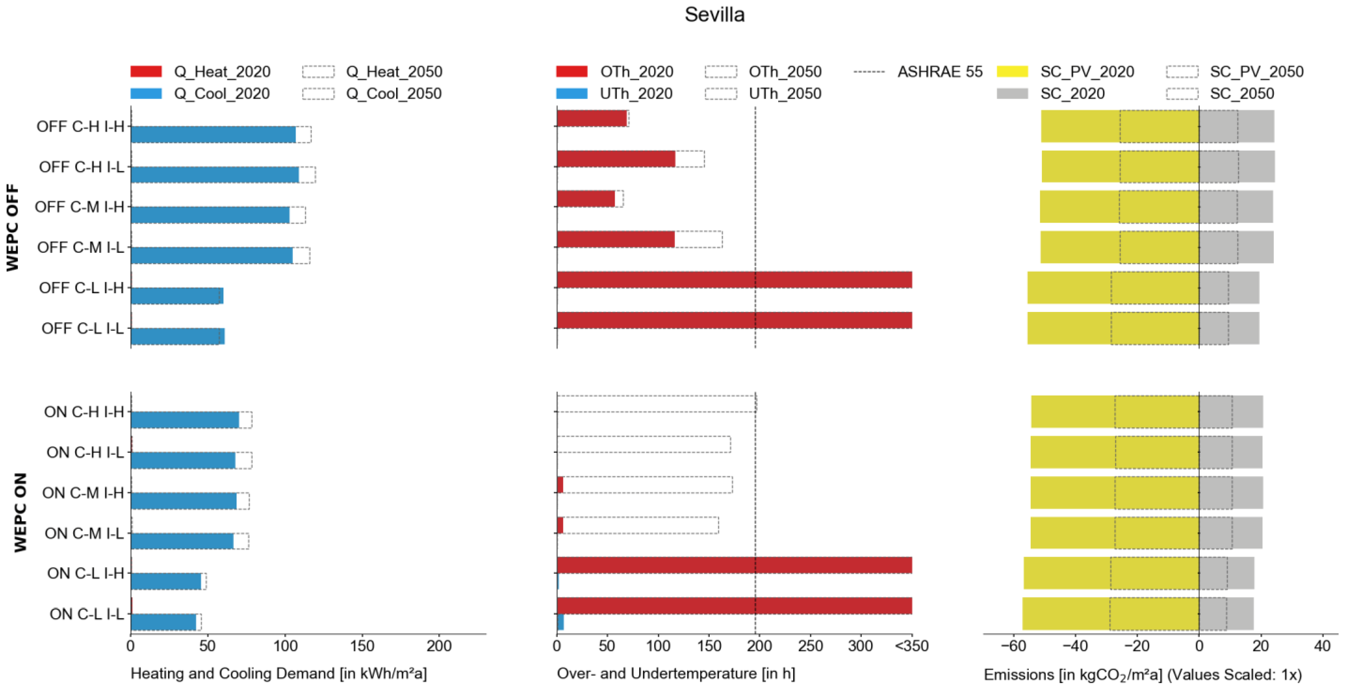
3.4. Hot Mediterranean Climate—Seville

In Andalusia’s hot climate, no heating demand is necessary, while cooling demand dominates with 40 to 110 kWh(m²a). Thus, all simulation variants have no noticeable UThs, while OThs exist in all cases. The light constructions cannot stay below the thermal comfort threshold. The highest cooling demand is needed with a standard control, high thermal mass, and low insulation, while the best-performing variant that fulfills the comfort is WEPC, middle–heavy, and low insulation. The middle and heavy constructions show only slight OThs based on the night cooling potentials of Seville. The permanently low EFs in the Spanish electricity grid lead to very few differences in emission performances, with SC +20 kgCO₂/(m²a), while the photovoltaics variants create energy savings around −55 kgCO₂/(m²a).

A decrease in thermal mass leads Seville to lower cooling demands, while a decrease in thermal insulation only slightly increases the cooling demand. The OThs are higher with less insulation but stay in range except for the light constructions. The emissions do not show a variation in the simulation variant categories. But, again, the overall trend of energy savings only exists with a PV and electrical storage and thermal storage system.

Overall, the WEPC variants perform better than their standard equivalent with 20–40 kWh/(m²a) less cooling demand and up to 50 h less OTHs, as displayed in Figure 16. In 2050, nearly all simulation variants show an increase of up to 10 kWh(m²a) in cooling energy demand and an increase in OThs. For the WEPC variants, the increase is slightly smaller. For heavy construction, the cooling energy demand rises more in absolute values. Future scenarios for SC and SC_PV decrease their permeances by ~50%. This is connected to the overall lower emission values in the Spanish electrical grid.

3.5. Cold Climate—Calgary

Calgary’s heating and cooling demands vary between 190 and 70 kWh/(m²a), with the highest variant with WEPC Off and a high thermal mass and low insulation, and the lowest with WEPC with a middle thermal mass and increased insulation. The cooling demand for all variants is between 5 and 15-kWh/(m²a) and therefore is neglectable. Thermal comfort can mainly be fulfilled except for the light construction variants and the simulation variant with WPC active, high thermal mass, and low thermal insulation, where the UThs are too high. The emissions in 2020 without PV showed similar results, differing around +80 kgCO₂/(m²a). The system configuration with PV presents emission savings of up to −90 kgCO₂/(m²a).

The less insulated simulation variants in Calgary show an increase in heating demand, while variants with a lower thermal mass show a decrease in heating demand. The cooling demand at 5–15 kWh/(m²a) is neglectable and stable for all simulation variants. Again, the trend of outperforming the WEPC is visible, as all WEPC variants use around 30–40 kWh/(m²a) less heating energy demand than their standard counterpart, especially for variants with heavy constructions. This reduction in energy results in an increase in UThs for the WEPC variants, but they mostly stay in the ASHRAE comfort range. The emissions with WEPC show around 10% less emissions, which results in around 12 kgCO₂/(m²a) less for SC and more emission savings for SC_PV.

The WEPC shows significant heating energy savings for the cold climate of Calgary and only in one case impairs thermal comfort. All future variants for 2050 show less heating demand based on the increasing temperatures in Alberta. This also decreases the UThs. Even with a slight increase in cooling energy and the OThs in the future, the authors consider a cooling system unnecessary. With more thermal mass, the heating demand will decrease more in the future. The emission savings decrease with the lower future EFs and increase the emission saving effect by 50%. All results are illustrated in the Figure 17.

4. Discussion

This discussion starts with the main findings of this work. First, an overview of the simulation results that prepares for the summarizing hypothesis is given, followed by answers to the individual research questions. Several universal validity trends can be observed based on the initially stated research questions and during this international parametric study. Finally, this section outlines the limitations of this work.

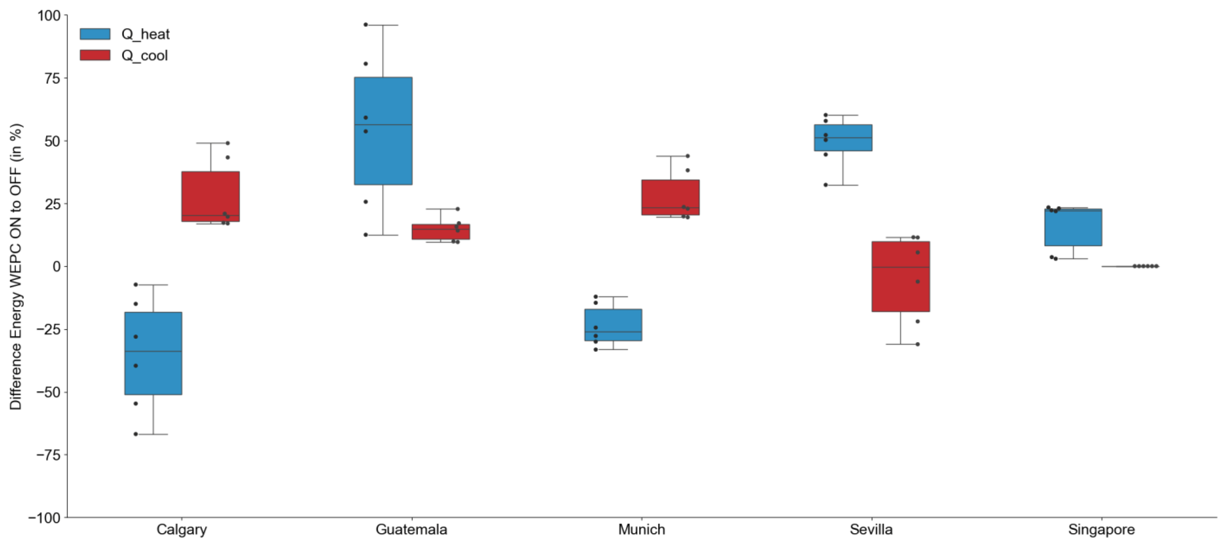
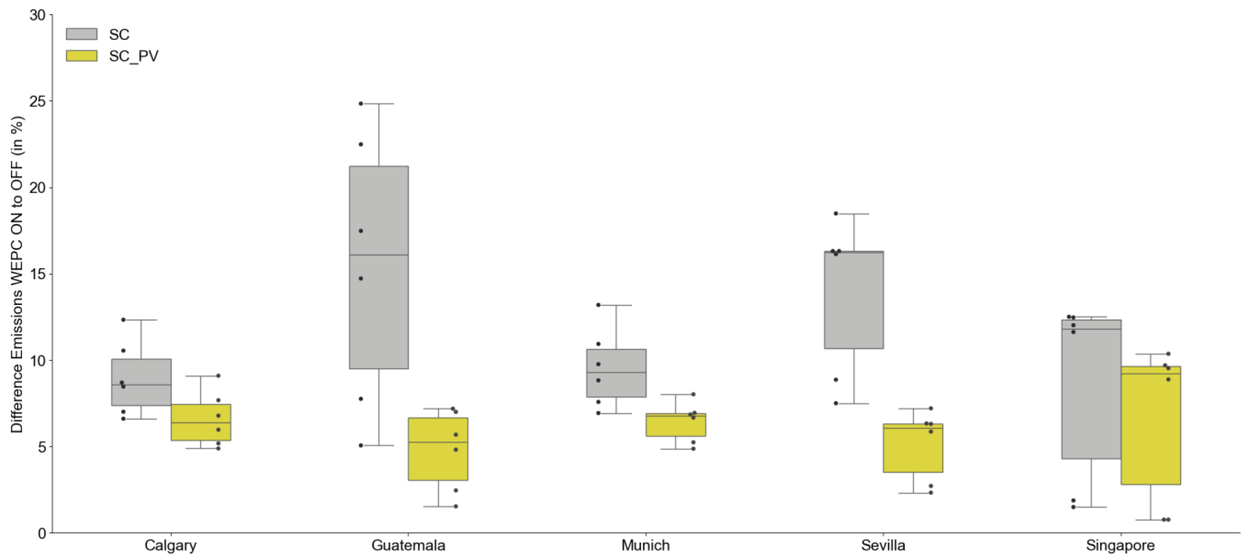
4.1. Main Findings

The ensuing two box plots show an overview of the simulation results, outlining the difference in energy and emissions between the equivalent simulation variants with WEPC On and Off for the five climate locations. Overall, one can see that the WEPC impacts heating, cooling, and emission performance. The single box elements of the graphs illustrate the range of the different performances for each climate location. The small, black dots represent the individual simulation variants.

Considering the energy performance in Figure 18, one can see that in all locations, but especially in Guatemala, where the variation in performance is very large, energy savings of around 50–100% can be archived with the WEPC. The emission performances in Figure 19 show similar results but with smaller ranges between 5 and 25%. Therefore, it is clearly visible that emission performances are more optimized without a PV system. This is linked to the personal use of solar energy with the PV system, which lowers the effect of the WEPC.

Summarizing the results for the individual climate locations shows that the overall hypothesis that a weather-and-emission predictive control of buildings improves the energy performance and the emission balance without limiting thermal comfort can be answered with yes, in many parts. Not all simulation results can archive improvements in all evaluation categories simultaneously, but an improvement is mostly detectable. These savings are sometimes represented in the energy or the emission savings. However, it is also clearly visible that energy savings do not always result in the same amount of emission savings and vice versa. This overall outcome proves that a simple control strategy, without a complex, data-intense approach, already creates energetic and emission improvements and protects from rebound effects and overengineering buildings.

• What impact does insulation and thermal mass have on the performance of the WEPC?

With increases in thermal mass, the heating and cooling energy demand rises. But, it prevents OThs and UThs, especially in the mornings when the building technology often cannot fulfill the thermal comfort requirements, according to ASHRAE 55 2004. The light construction variants mostly cannot fulfill the thermal comfort requirements except for the subtropical climate in Guatemala. Thus, one can see that TABSs does not perform well with light building constructions, except for the very pleasant subtropical climate. Increasing thermal insulation leads to a noticeable decrease in heating energy and often mildly decreases the cooling energy demand. This potentially results in fewer UThs but can also lead to more OThs.

• How does a photovoltaic system impact the emission balance using the WEPC with thermal and electrical storage?

For the system configuration with thermal and electrical storage, the emission factor is mainly determined by the emission values of the electrical grid. Negative emission values, thus emission savings, are only possible with owner occupancy of a photovoltaic system. However, the WEPC positively impacts the emission performances of both system configurations. The performances of SC and SC_PV can be improved by ~10% using the intelligent control WEPC.

• Does the WEPC improve a room’s energy performance and CO₂ balance without compromising thermal comfort?

In heating-dominant climate locations, WEPC creates significant energy savings. This also leads to improvements in emission performance compared to a standard control. The cooling demand can noticeably be lowered for Spain and Guatemala, but only small savings can be achieved in Singapore. This is found in the constantly high temperatures in the tropical climate without the possibility for night cooling or seasonal temperature decreases. Generally, a variation in the different simulation categories can only be achieved with fluctuating emission grids, as in Germany and Guatemala. Energy savings cannot always be transferred into emission savings, as storage systems also need to be controlled in an intelligent manner. Only small differences can be achieved in stable conditions, as is the case for Canada, Singapore, and Spain. With a flexible comfort concept like ASHRAE 55 2004, energy and, thus, emission savings are possible. The authors claim that more flexibility in thermal comfort in office buildings enlarges the saving potential.

• How does the WEPC perform in 2050, considering future weather and emission data that account for an increased share of regenerative energies?

In 2050, nearly all simulation variants show an increase of up to 20 kWh/(m²a) in cooling energy demand and an increase in OThs. The future heating demand will be lowered by up to 20% compared to 2020. This also decreases the UThs. The emission savings with photovoltaic systems decrease with the lower future EFs. This also reflects on the emission performances without photovoltaics and leads to a decrease of up to 50% in emissions. Overall, simulation variants with WEPC will show better emission and energy performance in the future than their standard equivalent. This strengthens the initial approach to simplify the control algorithms and proves that optimization with a simple approach like the WEPC is possible. It also creates advantages in future weather and emission scenarios.

4.2. Limitations

During the calculation and analysis, the authors had to set boundary conditions and make assumptions to complete this study. The ensuing paragraphs present the limitations of this approach, separated into building, comfort, emission, and weather aspects that should motivate further research. Still, overall, it must be noted that this study only analyses potentials and theoretical savings where further research has to put this concept into practice.

To fulfill the parametric study, several building assumptions had to be drawn to define the base case and the individual simulation variants. The very exposed office room set the base with its single façade, orientation, and very high window-to-wall ratio. Furthermore, the room’s geometry, infiltration, building technology system TABS, fixed PV area on the roof, and natural ventilation are set. A holistic parametric study needs to be conducted to identify the impact of each parameter. In addition, the quality of the simulation of the building technology and ventilation system is standard. Still, it could be extended with a detailed model of the building energy systems or a computational fluid dynamic simulation for the ventilation.

Furthermore, this study uses over- and undertemperaturehours, according to ASHRAE 55 2004, to evaluate thermal comfort conditions accurately. Further comfort concepts, such as a time-dependent thermal comfort, have other advantages that this study could not show. Other building uses, like residential or educational buildings with varying hours of occupancy and dress codes, could also be the focus of further research. In addition to that, it compromises the adaptive comfort band of ASHRAE, a wide range that supports the concept of WEPC, whereby other thermal comfort concepts would harm the results.

The dynamic emissions for this paper represent hourly values for the whole country, whereby, with an increase in renewable energies, the values can vary significantly in different regions of a country. Furthermore, the dynamic emission values are not integrated directly into the thermal simulation, as they are used in a second, separated simulation step. Predicting the emission values is found on a fixed decrease of emissions by 50%. This is a hard assumption and gives only a very-low-level prediction of emissions in the future. Overall, the boundary conditions of this study only comprise the emissions in the operational phase of the buildings, while constructive manners like thermal mass influence and demand for a holistic life cycle analysis of all building phases.

Finally, the weather data of the five climate locations use the TMY data sets to represent the general circumstances of a zone. Still, within the individual zones, various climates exist that could be represented with measured data. The findings of this study give an overall tendency for each climate zone but do not prevent further, detailed analysis. Lastly, the weather data prediction is based on the official IPCC scenario RPC 8.5. This represents a moderate baseline emission prediction scenario, whereby more extreme conditions can be expected with the ongoing trend of climate change.

5. Conclusions

This section outlines a conclusion of the concept of weather-and-emission predictive control. The underlying hypothesis is evaluated and analyzed in the following subsections: localization, utilization, and transformation of the potential. The authors of this paper reprise the hypothesis and present an outlook of this approach for future work.

5.1. Localization of the Potential

People use weather and emission data daily, preparing for their work life or planning a weekend trip into nature. As this paper outlines, weather and emission data hold great potential to optimize building operations. Previous studies also mention the possibility and the lack of application of such concepts that, in the authors’ opinions, are based on the complexity and inertness of data-intense control algorithms [9,10,11]. Building operation managers and even more building users are not experts in building data science and do not accept complex and expensive control algorithms. This opens the potential for this simplified building control approach for an application in the built world only found on simple calculations and an internet connection. Small devices like smartphones, Raspberry Pi, and thermostats can apply this. This simplicity is the basis for the potential of this approach, and this paper proves on a theoretical level the international energy and emission savings in various climates, especially when equipped with thermal mass and electrical storage systems in fluctuating electricity grids.

5.2. Utilization of the Potential

Using the WEPC for TABSs creates various energy and emission savings building variants in all five considered climate locations. Massive buildings, especially in heating-dominant places like Munich or Calgary, can save heating operational energy while fulfilling thermal comfort requirements. These savings increase with more thermal mass and less insulation. However, in Guatemala City, Sevilla, or Singapore, where a lot of cooling energy is required, the WEPC can slightly lower the energy and emission balance. Furthermore, this study confirms that locations with a higher variability when switching between heating and cooling modes (mainly within the transition from summer to winter) will increase the saving potential compared to the standard control for TABSs. In locations with a fluctuating emission factor with higher amounts of regenerative energies, like Germany or Guatemala, the WEPC with PV and an electrical storage system can decrease the operational emission balance. In locations with steady (high or low) emission factors, the WEPC only slightly outperforms a standard control strategy. Overall, the simple approach can decrease emissions and energy demand.

5.3. Transformation of the Potential

Ongoing climate change, in combination with the rising share of renewable energies, leads to a significant increase in the fluctuation of the energy price and emissions in the electrical energy grid. As the building energy supply is increasingly electrified, this rising fluctuation holds excellent potential for emission savings. This paper proves the necessity of innovative control strategies for building operations and the demand for more local storage systems. With the WEPC, buildings can be transformed into short-term energy and emission storages to support the concept of decentralization. The simulation variant with high thermal mass, an electrical storage system, and PV shows promising emission savings when using WEPC. But, also, Seville, representing an electrical grid with an all-year-long steady low emission, shows that with a low carbon emission still, an optimization using an intelligent control strategy is possible. To transform the potential of this study into the building stock, innovative control strategies have to focus on simplicity and be detached from high-tech solutions. Furthermore, the future scenarios with a substantial increase in renewable energy, especially in photovoltaics, outline that under ongoing climate change, the demand for storage systems will increase, and intelligent control strategies can enhance the saving potential. This strengthens the overall approach to simplify the optimization algorithms.

5.4. Outlook

Based on the broad findings and statements of this study, the authors identify steps to further develop the simple concept of WEPC and strengthen its application in the built world:

• Extend and reevaluate weather data prediction to further parameters to strengthen energy optimization.
• Extend the concept to the building design and the dimensioning of building technology to prepare for a whole life-cycling analysis considering emissions in all building phases.
• Develop and apply a more detailed future scenario algorithm for emission data to generate a better understanding of emission savings in the future.
• Apply the concept to a built energy system for revalidation.