Article

Advancing Fault Detection in Building Automation Systems through Deep Learning

1
AI Graduate School, Gwangju Institute of Science and Technology (GIST), Gwangju 61005, Republic of Korea
2
Aerospace Systems Design Laboratory, School of Aerospace Engineering, Georgia Institute of Technology, 275 Ferst Dr. NW, Atlanta, GA 30332, USA
*
Author to whom correspondence should be addressed.
Buildings 2024, 14(1), 271; https://doi.org/10.3390/buildings14010271
Submission received: 14 November 2023 / Revised: 19 December 2023 / Accepted: 9 January 2024 / Published: 19 January 2024
(This article belongs to the Topic Advances in Building Simulation)

Abstract

:
This study proposes a deep learning model utilizing the BACnet (Building Automation and Control Network) protocol for the real-time detection of mechanical faults and security vulnerabilities in building automation systems. Integrating various machine learning algorithms and outlier detection techniques, this model is capable of monitoring and learning anomaly patterns in real-time. The primary aim of this paper is to enhance the reliability and efficiency of buildings and industrial facilities, offering solutions applicable across diverse industries such as manufacturing, energy management, and smart grids. Our findings reveal that the developed algorithm detects mechanical faults and security vulnerabilities with an accuracy of 96%, indicating its potential to significantly improve the safety and efficiency of building automation systems. However, the full validation of the algorithm’s performance in various conditions and environments remains a challenge, and future research will explore methodologies to address these issues and further enhance performance. This research is expected to play a vital role in numerous fields, including productivity improvement, data security, and the prevention of human casualties.

1. Introduction

In today’s increasingly complex and interconnected world, the architecture of buildings and industrial facilities has undergone significant changes [1,2]. Not only have these structures expanded in scale, but the systems that manage them have become very complex [3,4]. This is driving the demand for sophisticated building automation and control systems [5,6,7]. BACnet is an essential component among the various protocols that drive this. It plays an indispensable role in seamlessly integrating and managing various subsystems, including heating, ventilation, air conditioning (HVAC), lighting control, and safety and security systems [8,9,10,11,12]. However, the complexity of these integrated systems creates a number of problems that are difficult to overlook [13]. Among them are mechanical anomalies and security vulnerabilities that can seriously compromise the reliability and efficiency of the entire system [14]. These problems can have a series of serious consequences, including productivity degradation, data leakage, and in extreme cases, loss of life [15,16]. Therefore, the main objective of this study is to develop a robust algorithm that can quickly and accurately detect mechanical anomalies and security vulnerabilities in building automation systems using the BACnet protocol. For this purpose, we utilized state-of-the-art machine learning algorithms and data analysis methodologies. These tools are used to design algorithms that can be monitored in real-time by learning anomalies and patterns of anomaly behavior. The second goal of this study is to extend the applicability of the findings. In addition to building management, we believe that this algorithm can be applied to various industries such as manufacturing, energy management, and smart grids [17,18,19]. This can greatly improve the universality of our findings. The main contribution of this thesis is the development and evaluation of a deep learning model for the real-time detection of mechanical faults in building network systems.
  • First, this research leveraged deep learning to develop a model that achieves significantly higher accuracy and efficiency than traditional fault detection methods, particularly through the process of adding noise to the data to improve the model’s generalization performance.
  • Second, the paper goes beyond simply detecting a single defect and presents a strategy that can cope with many different defect situations. This allows for high performance not only for single faults but also for complex multi-fault situations. This is of great practical significance as it provides concrete suggestions on how to maintain high performance in these various situations.
  • Third, the model developed in this study is designed for practicality and scalability. The model can be easily applied to real building network systems, allowing building managers or system engineers to make faster and more accurate decisions. This is expected to improve the reliability and efficiency of the overall building network system. Our model is designed to operate smoothly with the addition of new HVAC and AHU equipment to building network systems. This ensures efficient operation, even as the complexity and size of the system increase.
This paper consists of six chapters in total. Section 1, the ‘introduction’, details the background, necessity, and purpose of the study. In Section 2, ‘Related Work’, we review existing studies on anomaly detection and BACnet to explain how this work provides new value. Section 3 details the research ‘Methodology’ used in this study. One can learn more about how to collect and preprocess data, and how to design and implement the model. Section 4 focuses on ‘Experiments and Results’. It analyzes the various experiments conducted in this study and their results to assess whether the study objectives have been achieved. Section 5 ‘Discussion’ the limitations of the study results and the direction of future research. Through this, we would like to recognize the limitations of this study and suggest future research directions. Finally, Section 6 summarizes the main findings and ‘Conclusion and Future Work’ of this study. This paper proposes a new way to increase the reliability, efficiency, and scalability of building automation and control systems through this configuration and verifies its practical applicability.

2. Related Work

2.1. Machine Anomaly Detection Research

Machine anomaly detection continues to be a hot research topic in both industry and academia. In its early stages, anomaly identification was primarily based on statistical methodologies, analyzing simple characteristics and patterns in the data to identify anomalies [20,21]. While these approaches were effective for detecting simple and obvious anomalies, they were limited when it came to complex or unexpected anomalies. However, with the advancement of machine learning algorithms, various techniques such as Support Vector Machines (SVM), K-Nearest Neighbors (K-NN), and Decision Trees began to be increasingly applied to anomaly detection [22,23,24,25]. More recently, deep learning techniques, especially various forms of neural networks, have been excelling in anomaly detection [26,27]. These deep learning models are highly capable of handling high-dimensional and complex data and are also useful for real-time monitoring and prediction [28]. Machine anomaly detection is being used in a wide variety of applications, including industrial robots, manufacturing processes, and energy systems, which further emphasizes its importance [29,30,31,32,33]. Furthermore, anomaly detection is also an important research topic in network security and information security [34]. Initially, intrusion detection systems (IDS) primarily used rule-based methods to detect known attack patterns based on predefined rules [35]. While these methods performed well against known attack types, they were vulnerable to new types of attacks or complex attack patterns. Typically, there are “Zero-Day Attacks” using unknown vulnerabilities, or “Multi-Vector Attacks” that attempt multiple attacks simultaneously. To address this, new technologies such as anomaly-based analysis and state protocol analysis are being researched, and these approaches can identify more diverse and complex anomaly patterns by incorporating machine learning algorithms. These techniques, which perform well even on real-time data streams, can be utilized in a variety of applications and systems.

2.2. Research with BACnet
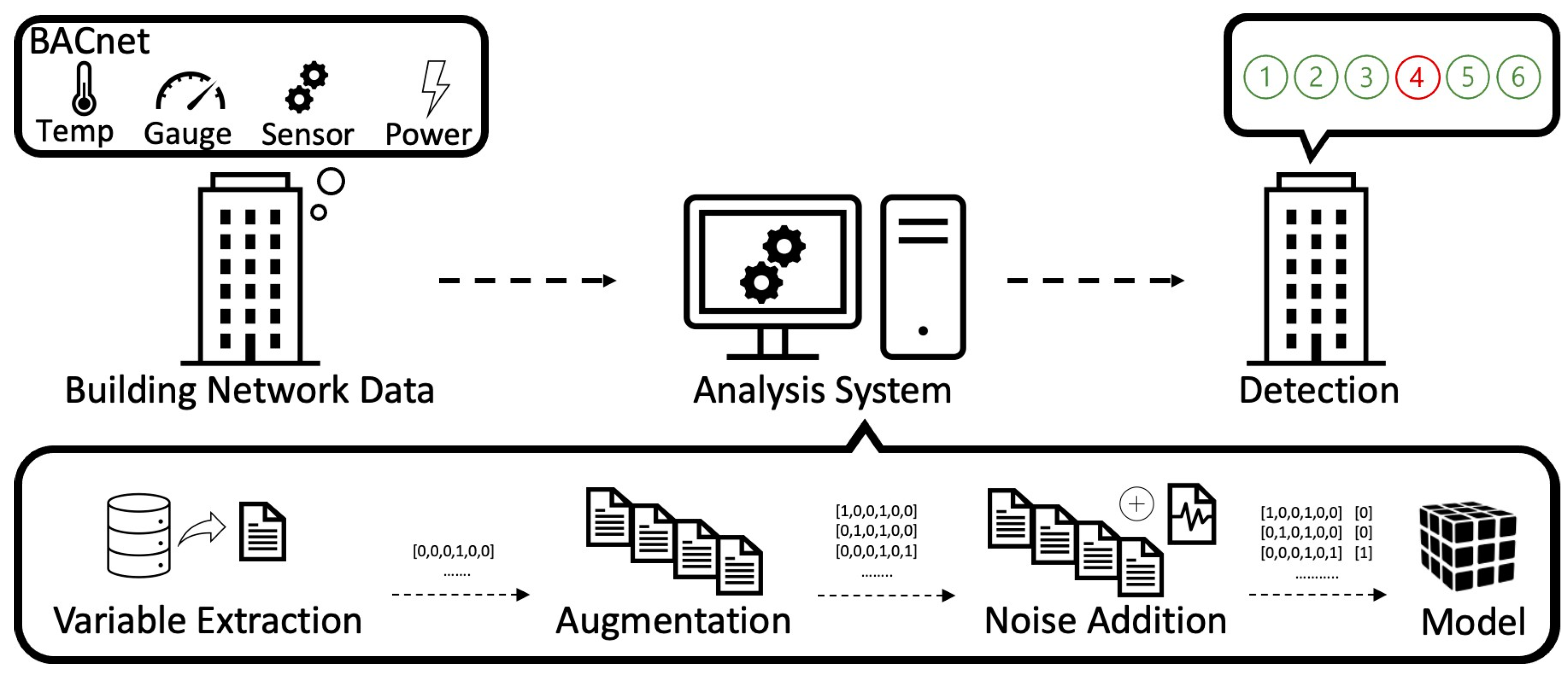
BACnet is a widely used protocol for building automation and control, initially focused on HVAC and lighting control [36]. It has since expanded to include energy management, smart grid connectivity, and Internet of Things (IoT) integration [37,38]. Kaur et al. focus on the BACnet protocol and list several possible attacks that can occur on BACnet networks, such as network flooding, traffic redirection, and rerouting [39]. Holmberg aims to raise awareness of the threats involved when connecting building control systems (especially BACnet systems) to a wider network. He presents countermeasures to combat security threats and provides information on current BACnet security and planned developments to improve security. The work also provides an overview of the use of firewalls, VPNs, intrusion detection systems, and security policies [40]. However, there is a relative lack of research on the security and anomaly detection aspects of BACnet. Most research focuses on the communication efficiency, compatibility, and scalability of BACnet, while the anomaly detection and security aspects are relatively neglected. Against this background, research on anomaly detection using BACnet is becoming increasingly important and requires the development of new approaches and algorithms.

3. Methodology

As shown in Figure 1, this study aims to develop a model that predicts and detects possible mechanical defects in real time within the building’s automation system and network. We focus on various types of mechanical faults that may occur in HVAC systems, Air Handling Units (AHU), and energy management systems. These faults can have catastrophic consequences, such as the inefficient use of energy or, in severe cases, damage to the system, making their prevention and rapid response critical. To build the model, we first collect health information on the building network and mechanical devices at 10 min intervals using high-performance sensors and data collection devices. The collected data are stored in a local database and used as the source data for further analysis. Based on this data, data preprocessing and feature engineering are performed to transform the data into a form that is easy to analyze.
As shown in Figure 2, this study demonstrates a model design that can detect mechanical failures using a total of 60 min of data, and this is performed by resampling and analyzing six consecutive data points every 10 min. The reason is that if failure occurs in an actual building operation situation, the impact accumulates over a period of time, so it is more accurate to comprehensively analyze the data over a period of time than to analyze simple instantaneous data. Because a minimum detection time of 10 min is set for each rule and interval A and interval B are compared, the fault lasts for a total of 60 min if the same fault occurs in six successive intervals (three A intervals and three B intervals). The maximum allowable time for the scenario set in this study is 1 h, and the time required to restore the system to its original state after the failure proposed by NREL is 2 h. In this study, we would like to use this methodology to propose a practical model for detecting mechanical failures in building networks that are expected to have a positive effect on the energy efficiency of buildings.

3.1. The Dataset

In this study, a special simulation platform was used to analyze the impact of cybersecurity threats on the building’s mechanical systems. The simulation is based on a reference building model from the U.S. Department of Energy (DOE), reproducing a cyberattack scenario through a log device. Network data and building physical health data obtained in this process provide great help in a clear understanding the real impact of cyberattacks and their causes. ‘A dataset of cyber-induced mechanical faults on buildings with network and buildings data’ [41] provided by NREL was first utilized. This dataset contains various mechanical conditions and network data for the building and has the advantage of reproducing complex real-world situations. Given these characteristics, it was considered a suitable dataset for the purpose of this study.
The simulation was run through a tool called ‘Alfalfa’, which not only allows you to query various pieces of state information of the building but also provides an interface function that applies external inputs to the model. This Alfalfa tool, in conjunction with the Building Automation System (BAS), centrally manages building health information and delivers necessary control commands to other BACnet devices. For example, BAS receives data from Alfalfa, such as building temperature, humidity, and energy usage, and controls BACnet devices such as air conditioners and dampers.
The dataset in this study comprehensively includes various variables and state changes that occur during these simulations, as well as the impact of malicious attackers on the system. Specifically, it contains detailed information about how an attacker distorts or interferes with BAS control commands and what mechanical faults occur in the building system as a result.
Table 1 is the ‘Experimental Scenario’ dataset provided by NREL that describes the various failure situations that occur in a building’s HVAC systems, and which includes the following key columns.
Table 2 shows that ‘Experimental Scenarios’ provides detailed information about various experimental conditions and variables. First, “Fault Expression” according to “Scenario Name” is also described in detail. Not only does this information help in a clear understanding of the situation each scenario is trying to simulate, but it also explains why it is important to predict the likelihood of failure conditions. Next, the item “Impact” analyzes in depth the potential impact of each failure situation on the building’s mechanical system. This analysis provides a credible basis for which cyberattacks can have a catastrophic impact on building systems. Finally, the “Cool Down” section specifies the time required to stabilize the system before applying the failure. In addition to designing experiments, this information serves as an important reference for developing effective response strategies to real-world cyber threat situations.

3.2. Data Analysis

As you can see in Table 3, each of the six Fault Names identified through data analysis has a different Fault Description, and they are categorized by relying on certain Variables. These ‘Variables’ are variables that are directly measured or monitored in the dataset to analyze the nature and cause of the fault. Therefore, the accurate measurement and monitoring of these variables plays a very important role in the correct detection and classification of faults. Therefore, the main objective of this research is the detection of six different ‘Fault Names’.

3.3. Variable Selection

In this study, only 13 important variables were selected from a total of 96 columns and used for analysis. This choice was based on several key reasons. First, high-dimensional data reduced the number of variables because they increased computational complexity and increased the risk of overfitting the model. Second, to clearly interpret the analysis results, we chose only the variables most directly related to the purpose of the analysis, excluding non-critical variables. Third, the fewer variables selected, the shorter the model’s learning and prediction time, resulting in more computational efficiency. Finally, to increase the reliability of the analysis, we removed unnecessary variables that could be noise. In this way, we were able to increase the efficiency and accuracy of our research at the same time.
Table 4 lists the 13 variables required for this study and their descriptions. These selected variables consider the building’s HVAC system, weather conditions, and various mechanical factors, and we believe they are well suited to the objectives of this study. The variable selection process was an important step in improving the predictive performance and computational efficiency of this study.

3.4. Characteristic Engineering

To determine the variables in the model, we focused on characteristic engineering. In this step, we selected and combined existing variables based on 13 previously selected variables. This can be valid for understanding the correlation between each variable and for various situations and conditions in complex building systems.
Table 5 adds extra variables, focusing on characteristic engineering. For example, we introduced a binary property that returns 1 if the value of a particular property exceeds a predefined threshold, or 0 otherwise. The new characteristics created in this way contributed to improving the predictive performance of the model.

3.5. Poisson Distribution

We calculated the probability of occurrence of each rule using Poisson distribution. This distribution quantitatively assessed the frequency and importance of the rules. The parameters of the distribution were set by referring to the characteristics of the dataset. The probability of k events in the interval, P X = k , is expressed as follows:
P X = k = λ k · e λ k !
where λ is the average rate of events per interval (also known as the rate parameter) and k! is the factorial of k.
The use of the Poisson distribution in our study is particularly justified due to its suitability in modeling the frequency of events in complex systems like building networks. This distribution is a perfect fit for several reasons. Firstly, the Poisson distribution is ideal for situations where events occur independently. In the context of building network systems, this is a crucial factor since faults and vulnerabilities, such as failures of “cooling coil valve fails” or “outside air damper is open”, usually occur without any direct correlation to one another. The Poisson distribution captures this aspect of independence effectively, allowing for a more accurate representation and analysis of these events. Secondly, the randomness of event occurrences in building networks is another critical aspect well-handled by the Poisson distribution. These systems are subject to a variety of faults and vulnerabilities that appear at unpredictable intervals. The Poisson distribution, with its ability to model random occurrences within a defined time frame, offers a reliable way to predict the frequency of these events. This ability to handle randomness is especially important for creating models that can anticipate and prepare for a wide range of potential issues. Additionally, the Poisson distribution is beneficial in quantitatively assessing the frequency and importance of different rules or events within the system. By setting the parameters of the distribution based on the characteristics of the dataset, it becomes possible to obtain a nuanced understanding of how often certain types of faults or vulnerabilities might occur. In summary, the choice of the Poisson distribution aligns well with the nature of building network systems, where faults and vulnerabilities occur independently and randomly. It provides a statistically sound method to handle the complexity of these systems and offers a way to estimate the probability of each event occurring more accurately. This makes the Poisson distribution an invaluable tool in our analysis, enhancing the overall reliability and effectiveness of our modeling approach.

3.6. Noise Addition

Adding noise is an important way to increase the generalization power of a machine learning model. Generalization means that the model is not limited to the training data, but also performs well on new data. This is very important because it determines how useful the model will be in the real world. Preventing overfitting is one of the main goals of adding noise. Overfitting typically results in poor performance, with new input as a model is excessively fitted by training data, resulting in poor performance on new data. By adding noise to prevent this, the model is forced to pay more attention to the general characteristics of the training data. Data augmentation is also an important purpose of adding noise. In situations where data are sparse, adding noise artificially increases the amount of data available, allowing the model to learn different patterns. Adding noise also has the effect of making the model more robust. Real-world data is often noisy, and training a model with noisy data improves the model’s robustness to that noise. In this study, we added a normally distributed noise with a mean of 0.5 to the training data to add noise similar to the distribution of the original data and a standard deviation of 0.001 to prevent the noise from overfitting the model without significantly affecting the original data. We also added noise by setting 5% of the total data as outliers, which allows the model to cope well with outliers and minor noise. This strategy has multiple benefits: it improves the model’s generalization ability, prevents overfitting, and makes it more robust to real-world data.

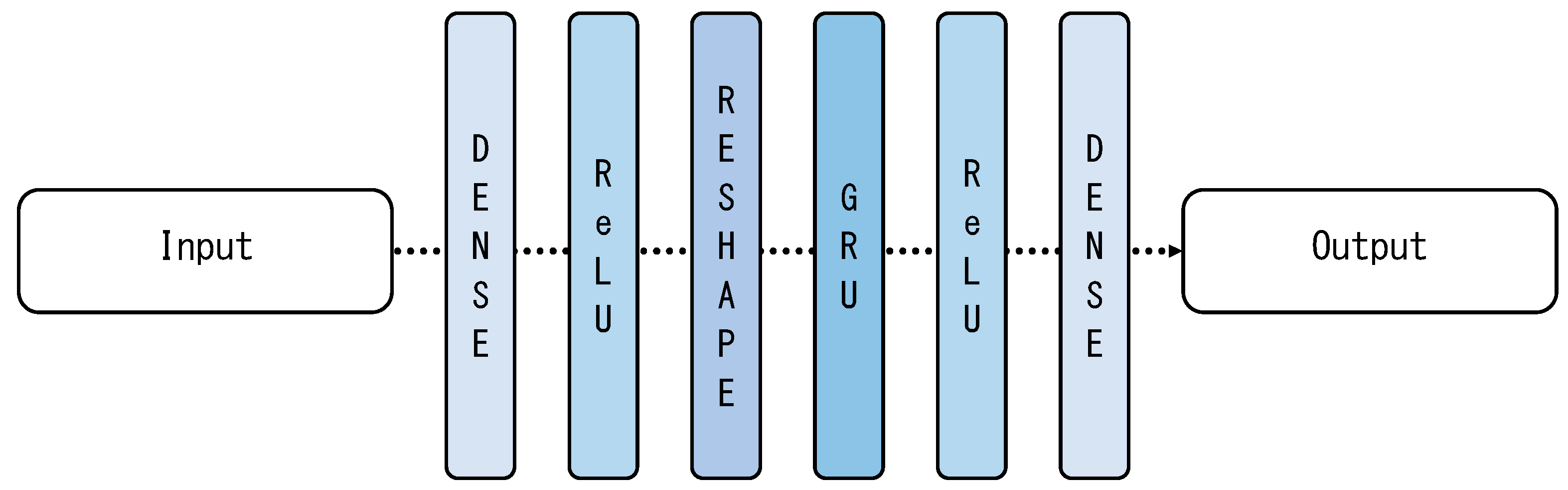
3.7. Detection Algorithm Model

As shown in Figure 3, this study contains the design of a deep learning model to effectively detect mechanical defects. First of all, we chose the most basic and widely used ‘simple random segmentation’ method as the data segmentation method. This method splits the entire dataset into training and test sets at random. Specifically, 80% of all data were allocated as training data and the remaining 20% as test data. This segmentation is known to help evaluate the generalization ability of the model by leveraging randomness to segment datasets evenly. We selected a model that combines multilayer perceptron (MLP), Gated Recurrent Unit (GRU), and Rectified Linear Unit (ReLU) as appropriate algorithms. This algorithm was deemed very suitable for the purpose of this study for several reasons. First, the multilayer structure allows the model to learn even complex patterns. This allows it to accurately model the various variables and interactions in the building network. Second, GRU cells can reflect the characteristics of time series data well. GRU efficiently utilizes historical information to predict current and future conditions, so it can accurately determine the impact of historical data on current mechanical faults. Third, enabling ReLU speeds up computation. This saves time in the training and inference phases of the model and can be applied to real-time flaw detection systems. Finally, the Adam optimization algorithm allows us to optimize the performance of the model quickly and accurately. For these reasons, we chose a deep-learning model based on this algorithm.
We chose Adam as the optimizer and used “categorical_crossentropy” as the loss function. The learning rate of the Adam optimizer was set to 0.005, which was deemed to be the most appropriate for the purpose of this study, as well as previous studies. To avoid overfitting the model and to achieve optimal performance, we also applied an early stopping technique, which automatically stops learning if the model’s performance does not improve over 20 epochs.

3.8. Model Performance Validation Metrics

3.8.1. Confusion Matrix

Table 6 is the Confusion Matrix. A confusion matrix is a visual representation of how well a model classifies. It is a fundamental tool for evaluating a model’s performance, providing basic elements such as True Positive, True Negative, False Positive, and False Negative. These elements provide the foundational information needed to calculate other performance metrics.
  • True Positive (TP): It’s Actually Positive, and the model classified it as Positive.
  • True Negative (TN): Actually Negative, and the model also classified it as Negative.
  • False Positive (FP): Actually Negative, but the model classified it as Positive.
  • False Negative (FN): Actually Positive, but the model classified it as Negative

3.8.2. Performance Metrics

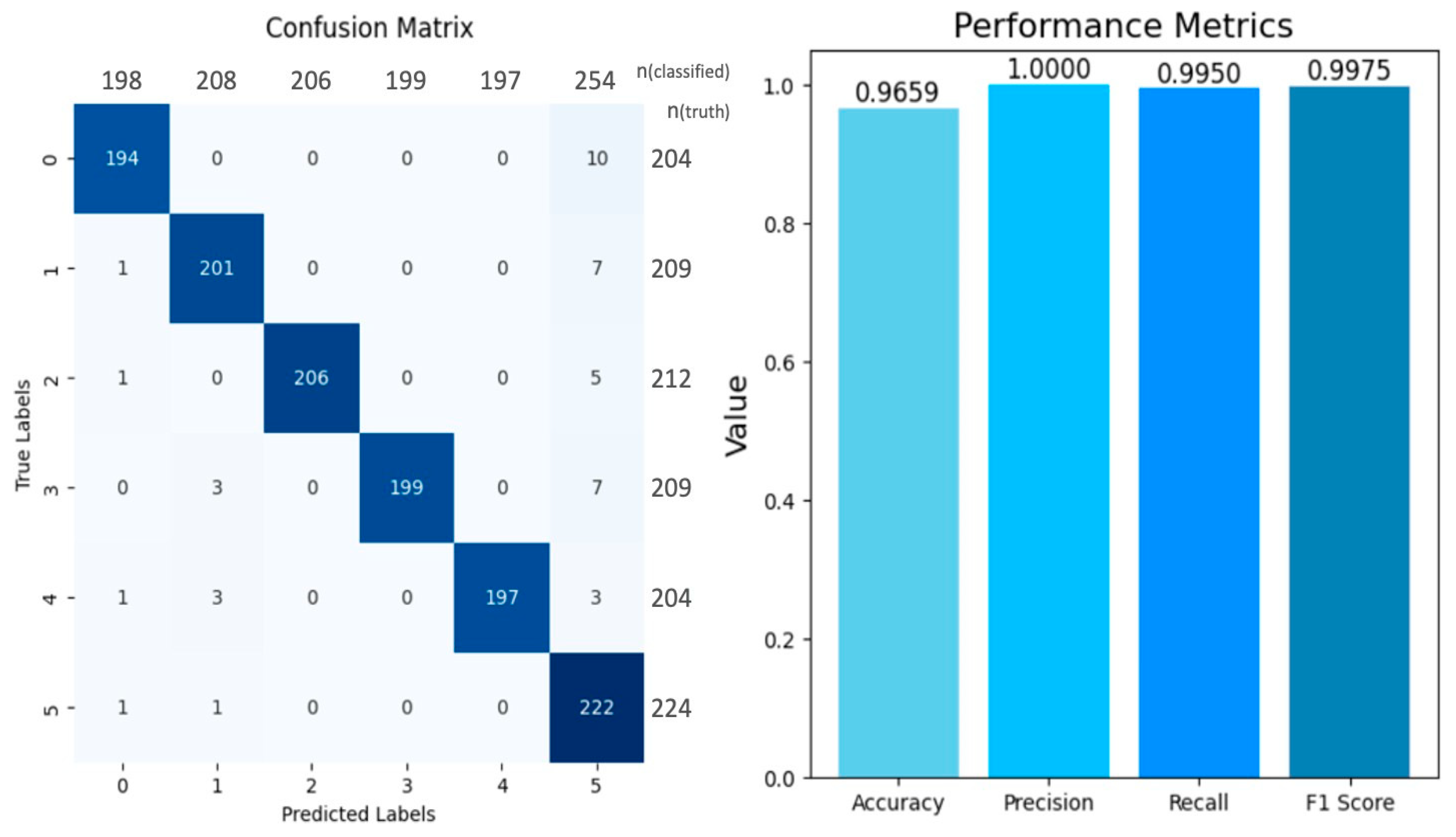
  • Accuracy is a metric that indicates how much of the total data the model correctly classified. This is the most intuitive metric to understand model performance, but it requires caution as it can be misleading if there is an imbalance in the data.
A c c u r a c y = T P + T N T P + T N + F P + F N
  • Precision refers to the percentage of data that the model classifies as positive that is actually positive. This metric is useful when it is important to reduce the number of false positives.
P r e c i s i o n = T P T P + F P
  • Recall indicates the percentage of data classified as positive by the model that is actually positive. This metric is useful when reducing the number of false negatives is important.
R e c a l l = T P T P + F N
  • F1 Score is the harmonic mean of precision and recall. This metric is used in situations where both precision and recall are important. When the two metrics are balanced, the F1 Score is higher.
F 1   S c o r e = 2 · P r e c i s i o n · R e c a l l P r e c i s i o n + R e c a l l
These performance metrics allow us to evaluate different aspects of how well our model actually works. Especially when it comes to the problem of detecting mechanical faults in building network systems in real time, these metrics are very useful for measuring the reliability and efficiency of our model.

4. Experiment and Results

In this study, we developed deep learning models to detect mechanical faults in building network systems in real-time. The experiments were based on data resampled every 10 min and successfully detected faults from a variety of situations and data. We used a Confusion Matrix and several Performance Metrics to evaluate and interpret the performance of these models.

4.1. Confusion Matrix and Performance Metrics

As shown in Figure 4, the performance of the deep learning model developed in this study for detecting mechanical faults in building network systems can be considered very high. From the confusion matrix, we can see that all the classes were classified very well: almost all the samples in each class were classified correctly. The performance metric also shows very high values. The accuracy is 96.59%, which means that the model made correct predictions in most cases. A precision score of 1 indicates that all the cases that the model classified as positive were actually positive. The recall and F1 scores were also near perfect. This high performance is likely due to the impact of adding noise to the data. Adding noise can contribute to improved performance because it improves the model’s ability to generalize and prevents overfitting.
As can be seen from Table 7, defect detection was performed for each of the six classes, and the results confirmed the high performance of the model. Accuracy, precision, recall, and F1 scores for each class were all high. These high-performance indicators suggest that the model can effectively detect even complex defect patterns. However, particularly noteworthy is the model’s performance in Class 6. In this class, precision was measured as relatively low, which makes it more likely that the model is over-detecting defects for Class 6. In fact, the number of samples classified by the model was significantly higher than the actual number of samples. This point indicates that the model may tend to overreact to Class 6. In addition, when viewed through the F1 score, the model maintains a good balance between precision and recall. This means that the model will show a stable performance even in real-world situations. In conclusion, although the model in this study shows high performance, it was confirmed that there is a need to improve the model in the future due to the relatively low precision of Class 6.

4.2. One Type of Defect Is Detected

This study is specifically designed to assume excessive situations. Specifically, while normal conditions remain in place for 60 h (3600 min), we model scenarios in which abnormal or malicious behavior occurs for a continuous hour (60 min). This design involves a class imbalance problem, but it was a deliberate choice. One of the main objectives of this study was to measure how quickly our model can detect anomalies in these excessive and realistic situations. This approach is significant for increasing model applicability in a variety of systems and applications where fast responsiveness in production environments is important.
In Figure 5, models specifically designed for experiments are set to detect only certain types of defects, and if a specific defect, such as “Cooling Coil Valve Stuck Closed”, is detected out of a total of six rules, it means that the cooling coil valve is operating in a closed state, which may not receive adequate cooling and therefore requires a prompt response. Because our model sets a detection time of at least 10 min for each rule, the actual detection time for the entire rule set is 60 min. In particular, if there are six successive sections (section A and section B), the fault lasts for a total of 60 min. If a defect in “Cooling Coil Valve Stuck Closed” is detected, ‘0’ in the variable column indicates that the rule or condition is inactive or undetected, whereas if only four columns display ‘1’, it means that those four conditions are active or detected.
If you detect only one type of fault, as shown in Table 8, you can create a response plan that is specific to that fault. This allows building managers or system engineers to take quicker and more accurate actions, contributing to a more reliable and efficient system.

4.3. Multiple Defects Detected

As shown in Figure 6, the model can detect multiple faults simultaneously, including ‘Cooling Coil Valve Stuck Closed’, ‘Heat Cool Operation without Min OA Damper’, and ‘OA Damper Stack Open’. This experimental setup is intended to simulate a situation where the cooling coil valve, the hot water valve, and the outside air damper are simultaneously causing problems. The model can accurately detect situations in which the same fault persists for 60 min in six successive sections with a slight lag (three A sections and three B sections that will occur in the future).
When three faults occur simultaneously, as shown in Table 9, they can have a very large impact on the building’s HVAC system. Therefore, it is essential to detect and analyze various faults simultaneously, especially since one fault is likely to trigger another. Therefore, such multi-fault situations require more thorough monitoring and a faster response, and it is important to analyze each fault independently and understand their interaction as much as possible. To this end, the model developed in this study is designed to provide detailed information about each fault, enabling effective responses in real-world operations.

4.4. Multiple Defects and One Insufficient Score Detected

In Figure 7, a number of defects, including ‘Cooling Coil Valve Stuck Closed’, ‘Cooling Coil Valve Stuck Open’, ‘OA Damper Stack Open’, ‘Low Supply Fan Speed’, and ‘High Supply Fan Speed’, occurred simultaneously with high probability. However, ‘Heat Cool Operation without Min OA Damper’ assumes a fault with a relatively low probability. The model can accurately detect situations in which a number of defects except one persist for a total of 60 min, even if the same defect occurs in six successive sections with a slight lag (three A sections and three B sections to occur). In addition, if one fault signal occurs during one unit of time (10 min), it can accurately detect at least six faults in 60 min.
These situations, like the one in Table 10, require particular attention. A fault detected with a high score indicates that a clear problem is occurring within the system and may require an immediate response. However, a fault detected with a low score, such as “Heat Cool Operation without Min OA Damper”, may be easy to ignore, but it may indicate that the cooling and hot water valves are not being regulated properly. This low score may be caused by the interaction with other faults or the influence of other system variables, which may lead to an increasingly large impact on the overall system. Therefore, these low scores are also significant and should be utilized in the evaluation of the overall system health. The model developed in this study is designed to flexibly respond to these different fault situations and score distributions. This will enable more accurate and efficient mechanical fault detection.

4.5. Not Detected

For Figure 8, we assume that a number of faults are rare with low probability over a unit of time (10 min). This can occur when the model collects data or when the equipment is switched. Because of this, it is highly likely that defects will not be detected in these situations.
If no failures are detected, as shown in Table 11, this can mean two possibilities. The system could be stable and fault-free. This is when the model is working correctly and has correctly determined that there are no faults. This situation can be a good indicator of the stability of the system. The system could be faulty but has not detected any faults. This situation requires attention. A situation where the model fails to detect a defect can be caused by a number of things. For example, a new type of fault might occur and the model might not recognize it. Or the model might misjudge the fault due to noise or the influence of other variables. Even when faults are not detected, periodic system checks and further analysis are still required, especially to ensure that the model’s performance is constantly monitored and updated as needed to ensure that no faults are missed.

5. Discussion

The deep learning model developed in this study showed very high accuracy in detecting mechanical defects in real time in building network systems. As a result of evaluation based on the confusion matrix and performance indicators, the model achieved an excellent accuracy of 96.59%. This indicates that the model performed accurate predictions in most situations. In addition, the precision, reproducibility, and F1 scores were all almost perfect, suggesting that the model has effectively learned different patterns of the data. The model demonstrated the ability to effectively detect not only single defects but also multiple defects. This is an important characteristic that allows us to respond quickly to complex problems that may arise in building network systems. In particular, with a detailed analysis by each class, the model showed excellent performance in distinguishing between different types of defects. According to the study results, the model maintained high performance even in the presence of noise added to the data, indicating that it could prevent overfitting and improve generalization capabilities in real-world environments.
However, since all results were limited to specific experimental conditions and datasets, further validation of the model’s performance in various real-world environments is needed. This study represents an important advance in the field of mechanical defect detection using deep learning, laying the foundation for a wider range of applications and performance improvements in the future.

6. Conclusions and Future Work

6.1. Conclusions

This study developed and evaluated a deep learning model to detect mechanical failures quickly and accurately in building network systems. Our model demonstrates the effectiveness of real-time defect detection with a high accuracy of 96.59% and an excellent F1 score, and in particular, it reduced the proposed ‘Cool-Down’ time by 50% compared to 2 h in the dataset provided by NREL, enabling anomaly detection within 1 h. This is a breakthrough that can significantly improve the efficiency of building management systems and quickly address potential risks. These results will be useful information for building managers. This means that shortening the failure detection process from 2 h to 1 h by applying the proposal in the dataset provided by NREL.

6.2. Future Work

Considerations for future research directions include the following. Model generalization and data extension considering data diversity are needed. The robustness of the model should be checked by verifying its performance in the real world as well as its performance in the experimental environment. In addition, the applicability of the model in other fields should be explored and the applicability in smart cities, manufacturing, etc., should be investigated. We expect that these studies will increase the practicality and field applicability of the model.

Author Contributions

Conceptualization, J.-H.L.; Methodology, W.-H.C. and J.-H.L.; Software, W.-H.C.; Validation, W.-H.C. and J.-H.L.; Formal analysis, W.-H.C.; Investigation, W.-H.C.; Resources, W.-H.C.; Data curation, W.-H.C.; Writing—original draft, W.-H.C.; Writing—review & editing, J.-H.L.; Visualization, W.-H.C.; Supervision, J.-H.L.; Project administration, J.-H.L.; Funding acquisition, J.-H.L. All authors have read and agreed to the published version of the manuscript.

Funding

This research was supported by the MOTIE (Ministry of Trade, Industry, and Energy) in Korea, under the Human Resource Development Program for Industrial Innovation (Global) (P0017311) supervised by the Korea Institute for Advancement of Technology (KIAT).

Data Availability Statement

This dataset, identified by ID 210 and accessible via DOI 10.7799/1922641, is publicly available and was last updated on 12 December 2023. It adheres to open data principles, ensuring transparency and availability for research and analysis purposes. The dataset is maintained and updated regularly, reflecting the latest findings and developments related to its scope. For further information, inquiries, or access requests, users are encouraged to refer to the dataset’s DOI link or contact the dataset’s custodian.

Conflicts of Interest

The authors declare no conflict of interest.

References

  1. Rivas Pellicer, M.; Tungekar, M.Y.; Carpitella, S. Where to Place Monitoring Sensors for Improving Complex Manufacturing Systems? Discussing a Real Case in the Food Industry. Sensors 2023, 23, 3768. [Google Scholar] [CrossRef]
  2. Waqar, A.; Skrzypkowski, K.; Almujibah, H.; Zagórski, K.; Khan, M.B.; Zagórska, A.; Benjeddou, O. Success of Implementing Cloud Computing for Smart Development in Small Construction Projects. Appl. Sci. 2023, 13, 5713. [Google Scholar] [CrossRef]
  3. Pan, Y.; Zhang, L. Integrating BIM and AI for smart construction management: Current status and future directions. Arch. Comput. Methods Eng. 2023, 30, 1081–1110. [Google Scholar] [CrossRef]
  4. Kor, M.; Yitmen, I.; Alizadehsalehi, S. An investigation for integration of deep learning and digital twins towards Construction 4.0. Smart Sustain. Built Environ. 2023, 12, 461–487. [Google Scholar] [CrossRef]
  5. Mishra, P.; Singh, G. Energy Management Systems in Sustainable Smart Cities Based on the Internet of Energy: A Technical Review. Energies 2023, 16, 6903. [Google Scholar] [CrossRef]
  6. Hepf, C.; Overhoff, L.; Koth, S.C.; Gabriel, M.; Briels, D.; Auer, T. Impact of a Weather Predictive Control Strategy for Inert Building Technology on Thermal Comfort and Energy Demand. Buildings 2023, 13, 996. [Google Scholar] [CrossRef]
  7. Dzyuba, A.; Solovyeva, I.; Semikolenov, A. Raising the Resilience of Industrial Manufacturers through Implementing Natural Gas-Fired Distributed Energy Resource Systems with Demand Response. Sustainability 2023, 15, 8241. [Google Scholar] [CrossRef]
  8. Graveto, V.; Cruz, T.; Simões, P. A Network Intrusion Detection System for Building Automation and Control Systems. IEEE Access 2023, 11, 7968–7983. [Google Scholar] [CrossRef]
  9. Apanavičienė, R.; Shahrabani, M.M.N. Key Factors Affecting Smart Building Integration into Smart City: Technological Aspects. Smart Cities 2023, 6, 1832–1857. [Google Scholar] [CrossRef]
  10. Márquez-Sánchez, S.; Calvo-Gallego, J.; Erbad, A.; Ibrar, M.; Fernandez, J.H.; Houchati, M.; Corchado, J.M. Enhancing Building Energy Management: Adaptive Edge Computing for Optimized Efficiency and Inhabitant Comfort. Electronics 2023, 12, 4179. [Google Scholar] [CrossRef]
  11. Skała, A.; Grela, J.; Latoń, D.; Bańczyk, K.; Markiewicz, M.; Ozadowicż, A. Implementation of Building a Thermal Model to Improve Energy Efficiency of the Central Heating System—A Case Study. Energies 2023, 16, 6830. [Google Scholar] [CrossRef]
  12. Almusaed, A.; Yitmen, I.; Almssad, A. Enhancing Smart Home Design with AI Models: A Case Study of Living Spaces Implementation Review. Energies 2023, 16, 2636. [Google Scholar] [CrossRef]
  13. Gao, Y.; Miyata, S.; Akashi, Y. Energy saving and indoor temperature control for an office building using tube-based robust model predictive control. Appl. Energy 2023, 341, 121106. [Google Scholar] [CrossRef]
  14. Jaramillo-Alcazar, A.; Govea, J.; Villegas-Ch, W. Anomaly Detection in a Smart Industrial Machinery Plant Using IoT and Machine Learning. Sensors 2023, 23, 8286. [Google Scholar] [CrossRef] [PubMed]
  15. Himeur, Y.; Elnour, M.; Fadli, F.; Meskin, N.; Petri, I.; Rezgui, Y.; Bensaali, F.; Amira, A. AI-big data analytics for building automation and management systems: A survey, actual challenges and future perspectives. Artif. Intell. Rev. 2023, 56, 4929–5021. [Google Scholar] [CrossRef] [PubMed]
  16. El-Kady, A.H.; Halim, S.; El-Halwagi, M.M.; Khan, F. Analysis of Safety and Security Challenges and Opportunities Related to Cyber-physical Systems. Process Saf. Environ. Prot. 2023, 173, 384–413. [Google Scholar] [CrossRef]
  17. Saleem, M.U.; Shakir, M.; Usman, M.R.; Bajwa, M.H.T.; Shabbir, N.; Shams Ghahfarokhi, P.; Daniel, K. Integrating smart energy management system with internet of things and cloud computing for efficient demand side management in smart grids. Energies 2023, 16, 4835. [Google Scholar] [CrossRef]
  18. Jafari, M.; Kavousi-Fard, A.; Chen, T.; Karimi, M. A review on digital twin technology in smart grid, transportation system and smart city: Challenges and future. IEEE Access 2023, 11, 17471–17484. [Google Scholar] [CrossRef]
  19. Giglio, E.; Luzzani, G.; Terranova, V.; Trivigno, G.; Niccolai, A.; Grimaccia, F. An efficient artificial intelligence energy management system for urban building integrating photovoltaic and storage. IEEE Access 2023, 11, 18673–18688. [Google Scholar] [CrossRef]
  20. Nakamura, T.; Imamura, M.; Mercer, R.; Keogh, E. Merlin: Parameter-free discovery of arbitrary length anomalies in massive time series archives. In Proceedings of the 2020 IEEE International Conference on Data Mining (ICDM), Sorrento, Italy, 17–20 November 2020; pp. 1190–1195. [Google Scholar]
  21. Hu, W.; Xiao, X.; Fu, Z.; Xie, D.; Tan, T.; Maybank, S. A system for learning statistical motion patterns. IEEE Trans. Pattern Anal. Mach. Intell. 2006, 28, 1450–1464. [Google Scholar]
  22. Piciarelli, C.; Micheloni, C.; Foresti, G.L. Trajectory-based anomalous event detection. IEEE Trans. Circuits Syst. Video Technol. 2008, 18, 1544–1554. [Google Scholar] [CrossRef]
  23. Akpinar, K.O.; Ozcelik, I. Analysis of machine learning methods in EtherCAT-based anomaly detection. IEEE Access 2019, 7, 184365–184374. [Google Scholar] [CrossRef]
  24. Tonkal, Ö.; Polat, H.; Ba¸saran, E.; Cömert, Z.; Kocaoglŭ, R. Machine learning approach equipped with neighbourhood component analysis for DDoS attack detection in software-defined networking. Electronics 2021, 10, 1227. [Google Scholar] [CrossRef]
  25. Olu-Ajayi, R.; Alaka, H.; Sulaimon, I.; Sunmola, F.; Ajayi, S. Building energy consumption prediction for residential buildings using deep learning and other machine learning techniques. J. Build. Eng. 2022, 45, 103406. [Google Scholar] [CrossRef]
  26. Copiaco, A.; Himeur, Y.; Amira, A.; Mansoor, W.; Fadli, F.; Atalla, S.; Sohail, S.S. An innovative deep anomaly detection of building energy consumption using energy time-series images. Eng. Appl. Artif. Intell. 2023, 119, 105775. [Google Scholar] [CrossRef]
  27. Chakraborty, D.; Elzarka, H. Advanced machine learning techniques for building performance simulation: A comparative analysis. J. Build. Perform. Simul. 2019, 12, 193–207. [Google Scholar] [CrossRef]
  28. Chung, S.H.; Ma, H.L.; Hansen, M.; Choi, T.M. Data science and analytics in aviation. Transp. Res. Part E Logist. Transp. Rev. 2020, 134, 101837. [Google Scholar] [CrossRef]
  29. Aldahiri, A.; Alrashed, B.; Hussain, W. Trends in using IoT with machine learning in health prediction system. Forecasting 2021, 3, 181–206. [Google Scholar] [CrossRef]
  30. Formosa, N.; Quddus, M.; Ison, S.; Abdel-Aty, M.; Yuan, J. Predicting real-time traffic conflicts using deep learning. Accid. Anal. Prev. 2020, 136, 105429. [Google Scholar] [CrossRef]
  31. Morariu, C.; Morariu, O.; Řaileanu, S.; Borangiu, T. Machine learning for predictive scheduling and resource allocation in large scale manufacturing systems. Comput. Ind. 2020, 120, 103244. [Google Scholar] [CrossRef]
  32. Castellani, A.; Schmitt, S.; Squartini, S. Real-world anomaly detection by using digital twin systems and weakly supervised learning. IEEE Trans. Ind. Inform. 2020, 17, 4733–4742. [Google Scholar] [CrossRef]
  33. Dairi, A.; Harrou, F.; Bouyeddou, B.; Senouci, S.M.; Sun, Y. Semi-supervised deep learning-driven anomaly detection schemes for cyber-attack detection in smart grids. In Power Systems Cybersecurity: Methods, Concepts, and Best Practices; Springer: Berlin/Heidelberg, Germany, 2023; pp. 265–295. [Google Scholar]
  34. Komisarek, M.; Kozik, R.; Pawlicki, M.; Choraś, M. Towards Zero-Shot Flow-Based Cyber-Security Anomaly Detection Framework. Appl. Sci. 2022, 12, 9636. [Google Scholar] [CrossRef]
  35. Zhang, J.; Zulkernine, M.; Haque, A. Random-forests-based network intrusion detection systems. IEEE Trans. Syst. Man Cybern. Part C (Appl. Rev.) 2008, 38, 649–659. [Google Scholar] [CrossRef]
  36. Kastner, W.; Neugschwandtner, G.; Soucek, S.; Newman, H.M. Communication systems for building automation and control. Proc. IEEE 2005, 93, 1178–1203. [Google Scholar] [CrossRef]
  37. Granzer, W.; Praus, F.; Kastner, W. Security in building automation systems. IEEE Trans. Ind. Electron. 2009, 57, 3622–3630. [Google Scholar] [CrossRef]
  38. Wetter, M. Co-simulation of building energy and control systems with the Building Controls Virtual Test Bed. J. Build. Perform. Simul. 2011, 4, 185–203. [Google Scholar] [CrossRef]
  39. di Vimercati, S.D.C.; Martinelli, F. ICT Systems Security and Privacy Protection. In Proceedings of the 32nd IFIP TC 11 International Conference, SEC 2017, Rome, Italy, 29–31 May 2017; Springer: Berlin/Heidelberg, Germany, 2017; Volume 502. [Google Scholar]
  40. Holmberg, D.G. Enemies at the gates: Securing the BACnet (R) building. ASHRAE J. 2003, 45, B24. [Google Scholar]
  41. Balamurugan, S.P.; Granda, S.; Haile, S.; Petersen, A. A Dataset of Cyber-Induced Mechanical Faults on Buildings with Network 537 and Buildings Data; Technical Report, National Renewable Energy Laboratory-Data (NREL-DATA); National Renewable Energy Laboratory: Golden, CO, USA, 2023. [Google Scholar]
Figure 1. Research overview.
Buildings 14 00271 g001
Figure 2. Anomaly detection models with resampled data.
Buildings 14 00271 g002
Figure 3. Algorithm model.
Buildings 14 00271 g003
Figure 4. Confusion matrix and performance metrics.
Buildings 14 00271 g004
Figure 5. One type of defect detected.
Buildings 14 00271 g005
Figure 6. Multiple defects detected.
Buildings 14 00271 g006
Figure 7. Multiple defects and one insufficient score detected.
Buildings 14 00271 g007
Figure 8. Not detected.
Buildings 14 00271 g008
Table 1. Description of columns in ‘Experimental Scenarios’.
Column NameDescription
ModelBuilding model name
WeatherSource of weather data
System LoopSystem loop (e.g., air side)
EquipmentRelated equipment (e.g., AHU)
Scenario NumberScenario number
Scenario NameName of the scenario
Fault ExplanationExplanation of the fault
Fault ExpressionLogical conditions to activate the fault
Required VariablesVariables required to determine the fault
Equivalent Point NameColumn name in the actual dataset corresponding to the required variables
ImpactPotential impact of the fault
WarmupTime required to stabilize the system before applying the fault
Attack Run TimeDuration the fault lasts
CooldownTime required to restore the system to its original state after the fault
Scenario SeasonSeason in which the fault occurs
Fault Injecting ScenarioMethod of injecting the fault
Expected ResponseExpected system response to the fault
Attack TypeType of attack causing the fault
Table 2. Part of the ‘Experimental Scenarios’.
Scenario NameImpactCool DownFault Expression
Cooling Coil Valve Stuck ClosedInsufficient cooling,
occupant thermal discomfort
2 hx = IF outside air temp > 35
& Supply air flowrate > 0
& Chilled water Valve Command > 50 pct
& (discharge air temperature
> discharge air temperature setpoint + 5)
for 30 min THEN 1 ELSE 0
Heat Cool Operation without Min OA DamperEnergy waste2 hx = IF Supply air flowrate > 0 is ON
& hot water valve command > 0
& chilled water valve command > 0)
for 15 min THEN 1 ELSE 0
Cooling Coil Valve Stuck OpenSpace over cooling,
occupant thermal discomfort, energy waste
2 hx = If Supply air flowrate > 0
& Chilled water Valve command = 0
& (discharge air temperature
< discharge air temperature setpoint - 5)
for 30 min THEN 1 ELSE 0
OA Damper Stack OpenEnergy waste2 hx = If unit is ON or Supply air flowrate > 0
& outside air damper command is CLOSED
& (abs (Return air temperature
- Mixed air temperature) > 5)
for 30 min THEN 1 ELSE 0
Low Supply Fan SpeedUnder heating/cooling2 hx = If Discharge Air Flows > 0
& Supply fan Speed command < 100%
& (discharge air Static Pressure
< discharge air Static pressure setpoint - 0.25)
for 1 h THEN 1 ELSE 0
High Supply Fan SpeedEnergy waste2 hx = If Discharge Air Flows > 0
& Supply fan Speed command = 100%
& (discharge air Static Pressure
> discharge air Static pressure setpoint + 0.25)
for 1 h THEN 1 ELSE 0
Table 3. Fault analysis table.
Rule_IdScenario_NameFault DescriptionVariables
1Cooling Coil Valve Stuck ClosedThis fault occurs when the cooling coil valve is closed, leading to insufficient cooling.weaSta_reaWeaTDryBul_y
hvac_oveAhu_yCoo_y
hvac_oveAhu_TSupSet_y
hvac_reaAhu_TSup_y
hvac_reaAhu_V_flow_sup_y
2Heat Cool Operation without Min OA DamperThis fault occurs when the cooling valve and hot water valve are both open, leading to energy waste.hvac_oveAhu_yCoo_y
hvac_oveAhu_yHea_y
hvac_oveAhu_yOA_y
hvac_reaAhu_V_flow_sup_y
3Cooling Coil Valve Stuck OpenThis fault occurs when the cooling coil valve is open, leading to excessive cooling.hvac_oveAhu_yCoo_y
hvac_reaAhu_TSup_y
hvac_oveAhu_TSupSet_y
hvac_reaAhu_V_flow_sup_y
4OA Damper Stack OpenThis fault occurs when the outdoor air damper is open, leading to energy waste.hvac_reaAhu_TMix_y
hvac_oveAhu_yOA_y
hvac_reaAhu_TRet_y
hvac_reaAhu_V_flow_sup_y
5Low Supply Fan SpeedThis fault occurs when the supply fan speed is too low, leading to insufficient airflow.hvac_oveAhu_dpSet_y
hvac_reaAhu_dp_sup_y
hvac_oveAhu_yFan_y
hvac_reaAhu_V_flow_sup_y
6High Supply Fan SpeedThis fault occurs when the supply fan speed is too high, leading to energy waste.hvac_oveAhu_dpSet_y
hvac_reaAhu_dp_sup_y
hvac_oveAhu_yFan_y
hvac_reaAhu_V_flow_sup_y
Table 4. Selected variables.
Variable NameExplanation
TimeTime Stamp of the Data
weaSta_reaWeaTDryBul_yOutside Dry Bulb Temperature from Weather Station
hvac_reaAhu_V_flow_sup_ySupply Air Flow Rate from AHU (Air Handling Unit)
hvac_oveAhu_yCoo_yCooling Command from AHU
hvac_reaAhu_TSup_ySupply Air Temperature from AHU
hvac_oveAhu_TSupSet_ySetpoint for Supply Air Temperature from AHU
hvac_oveAhu_dpSet_ySetpoint for Differential Pressure from AHU
hvac_oveAhu_yFan_yFan Status from AHU
hvac_oveAhu_yHea_yHeating Command from AHU
hvac_oveAhu_yOA_yOutside Air Command from AHU
hvac_reaAhu_TMix_yMixed Air Temperature from AHU
hvac_reaAhu_TRet_yReturn Air Temperature from AHU
hvac_reaAhu_V_flow_ret_yReturn Air Flow Rate from AHU
Table 5. Final variables.
Variable NameExplanation
TimeTime Stamp of the Data
weaSta_reaWeaTDryBul_yOutside Dry Bulb Temperature from Weather Station
hvac_reaAhu_V_flow_sup_ySupply Air Flow Rate from AHU (Air Handling Unit)
hvac_oveAhu_yCoo_yCooling Command from AHU
hvac_oveAhu_yFan_yFan Status from AHU
hvac_oveAhu_yHea_yHeating Command from AHU
hvac_oveAhu_yOA_yOutside Air Command from AHU
Extra_1hvac_reaAhu_TSup_y > hvac_oveAhu_TSupSet_y +5
Extra_2hvac_reaAhu_TSup_y < hvac_oveAhu_TSupSet_y - 5
Extra_3hvac_reaAhu_TRet_y - hvac_reaAhu_TMix_y > 5
Extra_4hvac_oveAhu_dpSet_y < hvac_reaAhu_dp_sup_y - 0.25
Extra_5hvac_oveAhu_dpSet_y > hvac_reaAhu_dp_sup_y - 0.25
Table 6. Confusion Matrix.
Prediction
PositiveNegative
ActualPositiveTPFN
NegativeFPTN
Table 7. Multi-class classification performance assessment metrics.
Classn (Truth)n (Classified)AccuracyPrecisionRecallF1 Score
020419898.89%0.980.950.97
120920898.81%0.970.960.96
221220699.52%1.00.970.99
320919999.21%1.00.950.98
420419799.45%1.00.970.98
522425497.31%0.870.990.93
Table 8. One type of defect detection result.
AnalysisExplanation
Predict_rule_id[1]
Detected FaultCooling Coil Valve Stuck Closed
Analysis_score[0.99994]
Sum_of_analysis_score0.99993997812227112
Table 9. Multiple defects detected result.
AnalysisExplanation
Predict_rule_id[1, 2, 4]
Detected FaultCooling Coil Valve Stuck Closed
Detected FaultHeat Cool Operation without Min OA Damper
Detected FaultOA Damper Stack Open
Analysis_score[0.99997, 0.9999, 0.99996]
Sum_of_analysis_score2.9998300075531006
Table 10. Multiple defects and one insufficient score detected result.
AnalysisExplanation
Predict_rule_id[1, 2, 3, 4, 5, 6]
Detected FaultCooling Coil Valve Stuck Closed
Detected FaultHeat Cool Operation without Min OA Damper
Detected FaultCooling Coil Valve Stuck Open
Detected FaultOA Damper Stack Open
Detected FaultLow Supply Fan Speed
Detected FaultHigh Supply Fan Speed
Analysis_score[0.99997, 0.71518, 0.99996, 0.99996, 0.99999, 0.99998]
Sum_of_analysis_score5.715039968490601
Table 11. ‘Not detected’ result.
AnalysisExplanation
Predict_rule_id[1, 2, 3, 4, 5, 6]
Analysis_score[0.0019, 0.117, 0.21459, 0.04307, 0.01659, 0.58922]
Sum_of_analysis_score0.9823699831031263
Disclaimer/Publisher’s Note: The statements, opinions and data contained in all publications are solely those of the individual author(s) and contributor(s) and not of MDPI and/or the editor(s). MDPI and/or the editor(s) disclaim responsibility for any injury to people or property resulting from any ideas, methods, instructions or products referred to in the content.

