1. Introduction
Since the last decade, the securitized real estate, which includes publicly traded real estate companies and real estate investment trusts, has yielded high returns for its investors, largely driven by the expansionary monetary policy with very low policy interest rates and large-scale open market bond purchases through quantitative easing programs [
1,
2,
3,
4]. Further, the underlying direct real estate market, as the world’s most significant store of wealth with a total value equating to more than all global equities and debt securities combined, plays a critically important role for the whole financial system and economy [
5]. Therefore, modeling and forecasting the risk of real estate is crucial for the stability of the financial and economic system [
6]. Volatility forecasting is a critically important step in investment, portfolio selection, security and derivatives valuation, risk management, and monetary policy making [
7,
8]. Therefore, modeling and forecasting real estate’s return volatility has been the subject of a large body of empirical and theoretical research, because volatility reflects and quantifies risk and uncertainty.
Further, the existing literature has found evidence of co-movements between securitized real estate and the underlying real estate market regarding their valuation, risk, and return [
9,
10]. More importantly, Ling and Naranjo [
11] find that securitized real estate leads direct real estate, since securitized real estate reacts to fundamental economic information faster than direct real estate does. In addition, long-term performance and securitized real estate are strongly related to direct real estate performance [
12] and volatility [
13]. Thus, modeling the securitized real estate index could inform and predict the risk of the whole real estate sector. However, most of the current real estate risk analyses that are carried out by both the media and policy makers are based on monthly data or even quarterly data of real estate transactions, which are highly lagged and do not effectively reflect the fundamentals of the real estate market in time. A securitized real estate index on a daily level is not used, mainly due to the complexity of the modeling and volatility pattern. This paper aims to address this problem by empirically testing the securitized real estate daily index in Sweden to understand the volatility pattern of return over time and identifying the most appropriate modeling framework for a developed real estate market.
Since the Scandinavian banking crisis of the early 1990s, the Swedish real estate industry has experienced three major economic crashes: the U.S. housing market crash and the breakdown of the subprime mortgage market which resulted in the 2007–2008 global financial crisis (GFC), the 2009–2012 European (sovereign) debt crisis (EDC), and the ongoing global COVID-19 pandemic. These crises have negative impacts on the financial market and economy. In this paper, we focus on the dynamic volatility behavior of the daily Swedish Real Estate Sector Index and analyze the existence and the degree of a long-range dependence or asymmetric news effect from January 2003 to June 2021, with a special focus on these extreme events. We follow the literature to adopt a wide array of approaches based on the standard Generalized Autoregressive Conditional Heteroscedasticity (GARCH) approach [
14] and its popular extensions to model the volatility pattern of the daily returns of the Swedish Real Estate Sector Index. Then, we compare and evaluate the (out-of-sample) volatility forecasting performance of the various estimated GARCH models to identify the optimal model for the real estate sector in Sweden. As far as we know, this is the first paper that investigates the volatility behavior of the Scandinavian real estate sector.
Our results show that the volatility of the Swedish Real Estate Sector Index is time-varying and highly volatile. The impacts of the global financial crisis, European debt crisis, and COVID-19 pandemic are noticeable. Moreover, the volatility pattern during the COVID-19 period displays significant time-varying long-range dependence and an asymmetrical news impact, which lead to market inefficiency. The volatility pattern shows a tendency towards increasing leverage effects and less persistent behavior. This indicates that market stakeholders are highly sensitive to negative returns and respond to market changes much quicker. Moreover, we have applied a comprehensive model selection criterion and concluded that the most suitable method during the in-sample period does not have the same accuracy during the forecasting process, which has enriched the current empirical literature.
This article starts with a comprehensive literature review on applying various GARCH models to financial assets.
Section 3 introduces the theoretical framework of basic GARCH models, asymmetric GARCH models, and long-memory GARCH models with distribution functions, model diagnostics, and analysis for both the fitting and prediction phases.
Section 4 describes the data and presents the in-sample results.
Section 5 provides the out-of-sample forecasting results (including VaR backtesting). Finally,
Section 6 summarizes our findings and offers a conclusion.
3. Methodology
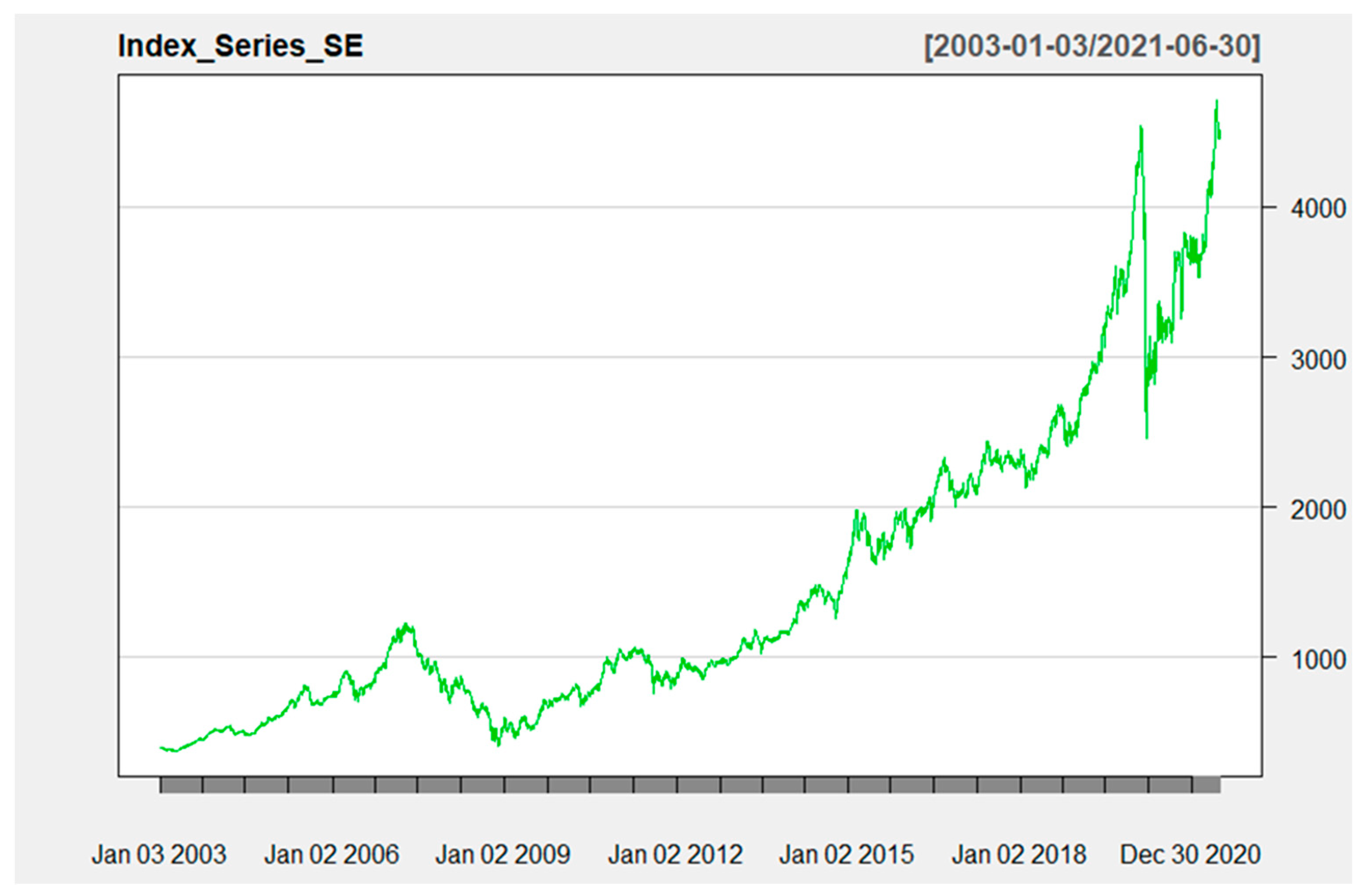
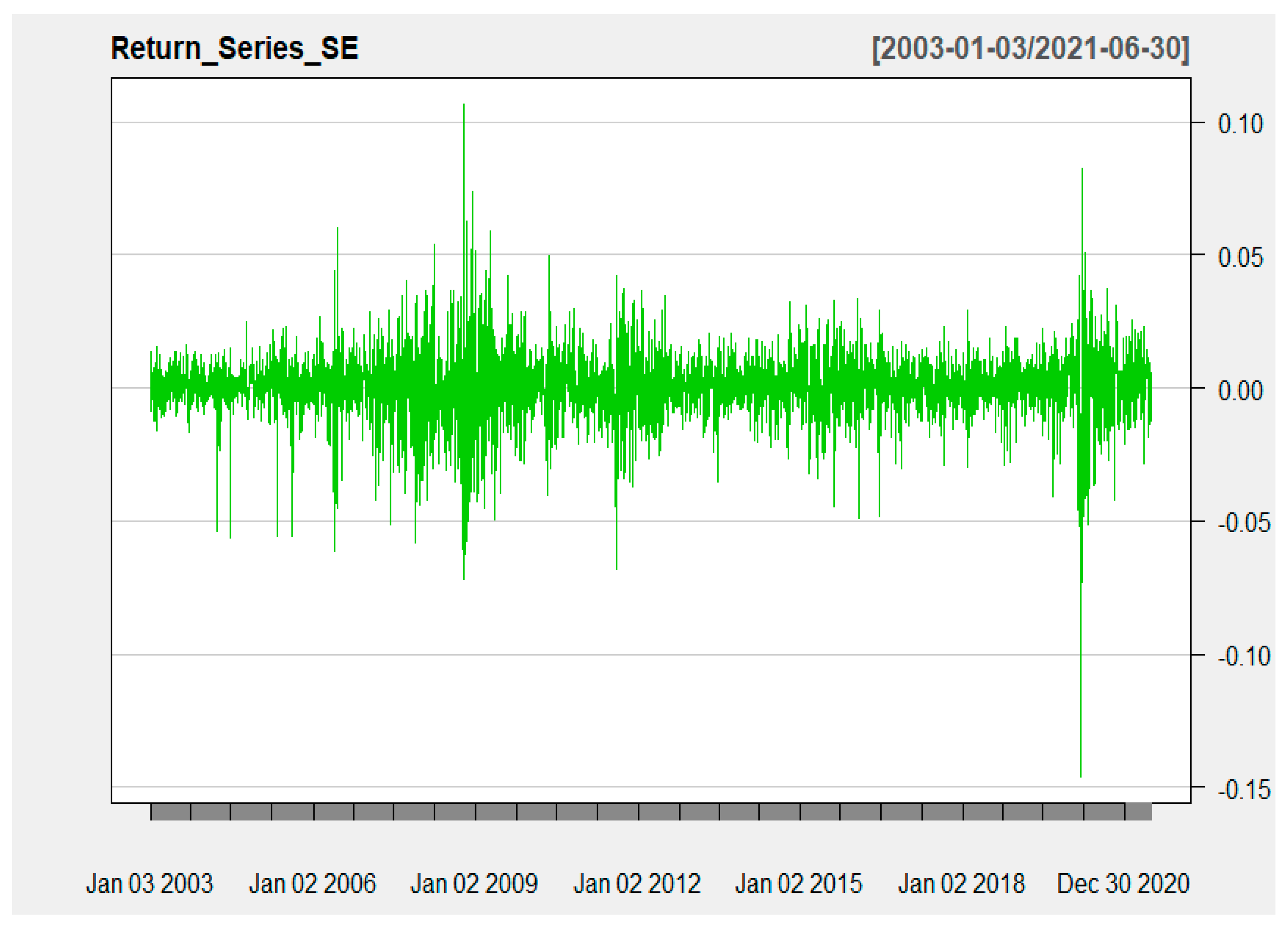
The time series data of Swedish Real Estate Sector Index daily returns shows clear evidence of time-varying volatility and clustering, as shown in
Figure 1 and
Figure 2. In some time periods, the volatility is mostly low (e.g., 2003–2006 and 2016–2019), while the volatility is much higher during the 2007–2008 financial crisis and during 2020, when the world economy and the financial markets were hit by the COVID-19 pandemic. Also, the volatility is higher during the 2009–2012 European debt crisis. Thus, the data show that periods with smaller return volatility are followed by further small changes in volatility, and periods with larger return volatility are followed by further large volatility. It is this pattern that is typical for time-varying volatility, as well as volatility clustering.
GARCH models are very popular because they are useful for modeling time-varying volatility. In this methodology section, we briefly summarize the econometric specifications of the time-varying volatility models, that is, the various GARCH models that are assessed in this paper. For a more detailed introductory explanation of the GARCH models and their specifications, see, e.g., [
6]. In short, the GARCH models capture the evidence of volatility changes and clustering via lagged-return news or shocks and the momentum of such shocks (e.g., the initial COVID-19 return shocks resulted in higher return volatility not only in the first days but also in the coming days).
3.1. Basic GARCH Model
The benchmark model is the Generalized Autoregressive Conditional Heteroscedastic (GARCH) model that was proposed by Bollerslev [
14] in 1986. Specifically, a GARCH (p, q) model is defined as follows:
The GARCH model reflects that the variance at time t, changes with both the lagged effect of news or shocks via the squared return error term, for j = 1,…, p lags, and via the lagged variance for i = 1,…, q lags. In this model, α is the random influence from the previous period, and β measures the lagged past variance. A large α reflects a significant reaction to market movement, while a large β indicates the shock of the fact that conditional variance takes a longer time to die out (i.e., news or shocks have a momentum effect, implying that news are persistent). Given the variance equation, expresses the conditional volatility of the return series at time t.
Since the standard GARCH (1, 1) model, where p = 1 and q = 1, is the most extensively applied and examined model in the literature, we have used this model as our benchmark. Regarding the mean equation, denotes the return of the sector index at time t, and is the mean of given the information from the past period t − 1,…,. m is the order of the autoregressive process (AR-process) with k = 1,…, m lags of returns, and n is the order of the moving average process (MA-process), with l = 1,…, n lags of the error term.
Volatility model parameters are assumed to follow the restriction and the constraints are applied to ensure that σ2 is strictly positive; meanwhile, holds.
The return of a financial time series may depend on its volatility or variance. To model this phenomenon, the Generalized Autoregressive Conditional Heteroscedastic-in-Mean (GARCH-M) model could be applied.
The GARCH-m equation has an extra heteroscedasticity term as , where γ is called the risk premium parameter and is the ARCH-in-mean effect, and k = 1 for volatility in mean and k = 2 for variance in mean. A positive τ indicates that the return is positively related to its volatility or variance. In other words, the rise in the financial time series means that the return is caused by the increase in the conditional variance. The modified ARMA process allows for volatility feedback on conditional expected returns and shows the influence of volatility on mean.
3.2. Asymmetric Conditional Volatility Models
During the volatility-generating process, the impact of the negative and positive information of the series could be critical and asymmetric. However, the basic GARCH (p, q) model is unable to capture the asymmetric volatility reaction towards good news (returns being higher than expected) and bad news (returns being lower than expected). The EGARCH model (Exponential GARCH (p, q) model) is improved by Nelson [
43] to consider the leverage effect, with a special variable to distinguish the negative and positive impacts, as per the following form:
where
is the conditional volatility of the return series at time t,
measures the sign effect—if
is negative, bad news shocks will have a greater impact on volatility—and
captures the size effect. Thus, the persistence of the autocorrelation in the GARCH (p, q) model is measured by α + β, while only β in the EGARCH (p, q) model reflects the decay rate.
The GJR-GARCH model developed by Glosten et al. [
44] models good news and bad news as follows:
where
And is the leverage term, while all other parameters are as previously defined.
Another commonly used volatility model is the asymmetric power ARCH model developed by Ding et al. in 1993.
where
> 0, and −1 <
< 1 is the leverage parameter. If
, the positive shock and the negative shock will have the same effect on conditional volatility. A positive
value indicates that leverage presents, and negative returns increase, while σ indicates more negative returns than positive returns.
3.3. Long-Memory Volatility Models
For short-memory models, the correlation of the series and its lag converge to a constant when the lag becomes large. On the other hand, the effects of volatility shocks decay slowly in long-memory models. Financial assets tend to display a high persistence in terms of their volatility, where autocorrelation exists over long lags. But a long memory in financial time series is subject to further theoretical and empirical research. The above mean and variance models are for short-memory processes in order to study whether long-memory processes produce better explanations and forecasts. We have selected the integrated GARCH (IGARCH) model, which is specified by Engle and Bollerslev [
45] and Baillie et al.’s [
46] Fractionally Integrated GARCH, or FIGARCH:
where L denotes the lag or backshift operator, and where 0 ≤ d ≤ 1. When the fractional differencing parameter d gets closer to 1, the memory of the FIGARCH increases; when d = 0, the FIGARCH is reduced to standard GARCH; and when d = 1, FIGARCH transforms to an integrated GARCH (IGARCH) model. In the IGARCH model, the unique feature of the model specification is the infinite memory, which means that the volatility shock is permanent and affects all horizons. However, a never die out assumption seems unrealistic. Thus, FIGARCH employs a more flexible class of processes for the conditional variance and captures the long-memory features of financial volatility through parameter d.
3.4. Model Evaluation Using Loss Functions
To estimate the parameters, the maximum likelihood (MLE) technique is applied under the assumption that the residual
follows a conditional Gaussian (normal) distribution. We have chosen a normal distribution as our default, which other distribution assumptions, for example, Student’s-t distribution, skewed Student’s-t distribution, and GED distribution, will replace. Quasi-maximum likelihood (QML) is applied when normality is violated to yield consistent parameter estimates [
47,
48]. To evaluate the suitable density function, we used the Bayesian information criterion (BIC) and Akaike information criterion (AIC) together with the value of log-likelihood. Furthermore, the BIC and AIC criteria are also applied in mean and variance models to select different orders of p and q. Models with the smallest AIC and BIC values are considered to have the best fit.
To evaluate the forecasting ability that different models produce, we have selected both mean absolute error (MAE) and mean square error (MSE) methods. The two approaches are calculated as follows:
where
is the forecasted volatility,
represents the true volatility, and n is the total number of forecasts. The model with the lowest MAE and MSE value implies the most accurate forecasts.
3.5. Model Evaluation by Backtesting Value-at-Risk (VaR)
It is common that GARCH models are used to estimate Value-at-Risk (VaR) models. VaR calculations are performed by financial institutions to quantify the risk of investments and therefore used as a risk management tool [
6]. Since volatility, and above all, time-varying volatility, of investment returns, are important determinants of the level of risk of investments, the use of various GARCH models to estimate VaR is popular. Furthermore, it is common that financial institutions backtest VaR calculations (using historical return data) to analyze whether their VaR calculations are accurate. Therefore, we also evaluate GARCH model specifications by backtesting VaR. The test procedures are from Kupiec’s test [
49], which is used to evaluate GARCH specifications for conditional coverage tests, and the independence test (conditional coverage test) introduced by Christoffersen [
50].
The indicator variable
is used to measure whether there is an observed actual VaR that exceeds the VaR estimations:
where
follows the binomial distribution. Let α be the significance level, sample size T, and N is the sum of
, which counts actual days of failure. The failure rate can be expressed as
.
Based on Kupiec’s proposal in 1995 [
49], the likelihood ratio test (
can be performed with
, and the statistic is given as
where
under the null hypothesis, the 95% confidence level has a critical value of 3.84. Thus, H_0 is rejected if the
value is larger than 3.84 with a
p-value of
that is smaller than 5%, indicating a less appropriate model specification.
VaR estimation is based on the assumption that failures are independently distributed over time. Assuming that the model is well specified, today’s violation does not depend on yesterday’s conditions, which means that these variables should be independent and identically distributed (i.i.d.) over time. However, Kupiec’s LR test focuses mainly on the number of violations. Thus, Christoffersen proposed the conditional coverage test in 1998 [
50], which can test both frequency and independence through a likelihood ratio test (
). The test statistic is given as
where
is the probability of observing a violation at time t when
occurred at t−1.
is the number of days where
followed by
.
follows the χ
2 (2) distribution under the null hypothesis with a critical value of 5.99 at a 5% significance level. Given a 95% confidence level, the null hypothesis is rejected if the
p-value of the
statistic is smaller than 5%. This section may be divided by subheadings. It should provide a concise and precise description of the experimental results, their interpretation, as well as the experimental conclusions that can be drawn.
4. Data
Most of Sweden’s largest real estate companies are listed on Nasdaq OMX Stockholm. This section presents the descriptive statistics of the daily index values and returns in the OMX Real Estate Sector Price Index, designed to track the listed real estate companies in Sweden. The dataset consists of 4642 daily observations, which have been obtained from Nasdaq Global Indexes.
The total sample period spans from January 2003 to June 2021 and covers three substantial financial and economic crises, namely, the global financial crisis (GFC), the European debt crisis (EDC), and the COVID-19 pandemic (COVID-19). Therefore, the index series has been divided into five subsamples: before the global financial crisis (the pre-GFC) period (January 2003 to June 2007), during the GFC (July 2007 to September 2009) [
51,
52,
53,
54], during the European debt crisis period (October 2009 to December 2012) [
55,
56,
57,
58,
59], the post-EDC period (January 2013 to January 2020), and the COV19 (January 2020 to present) period.
The first 90% of each period is selected as an in-sample, while the remaining 10% is an out-of-sample. We use the in-sample period for volatility estimation and the out-of-sample period to analyze the forecasting ability of competing models.
The daily returns are calculated as the first difference of the log index, given by
where
is the return of index i at time t, and
and
denote index i at time t and time t − 1, respectively.
Figure 1 shows the daily real estate index price trend (top graph) and daily log returns (bottom graph) of the OMX Real Estate Sector Index from January 2003 to June 2021.
Descriptive log return statistics for the indices are given in
Table 1.
Table 1 gives an overview of the return and risk levels of the full sample and five subsamples. Apart from the GFC sample, all samples have a very small positive mean return compared to the standard deviation, which is unconditional volatility. Similar to other financial assets, the full sample series exhibits negative skewness and excess kurtosis. As for subsample COVID-19, the return series displays the highest uncertainty level and kurtosis. The minimum value of the daily return is −14.6%, which is on Black Thursday, 12 March 2020.
The null hypothesis of the Jarque Bera Test shows that returns are distributed normally, which is rejected at a 1% significance level in all cases. The ARCH-test results confirm that heteroscedasticity is inherent in all series, where periods of high volatility tend to follow periods of high volatility, and periods of low volatility are also clustered.
5. Empirical Results
5.1. Estimation of Volatility Measurements
We firstly adopt the ARMA (p, q) process to estimate the residual as the measures of volatility.
Table 2 displays the estimated ARMA (p, q) process, and AIC is applied to detect preferred lag orders.
As we can see in
Table 2, the preferred order for ARMA (p, q) differs for each sample. Thus, ARMA (2, 0), ARMA (1, 1), ARMA (1, 0), ARMA (1, 2), ARMA (1, 0), and ARMA (1, 1) are selected for mean equations correspondingly.
Table 3 presents the result of each sample’s density function selection of the ARMA (p, q)-GARCH (1, 1) model. Normal distribution assumptions are not fulfilled for all series. Skewed functions outperformed non-skewed functions in all series except for the GFC subsample.
5.2. In-Sample Estimation and Evaluation for the Full Sample
We used the first 90% of the Swedish Real Estate Sector Index observations from the full sample, January 2003 to June 2021, to fit with the 12 GARCH family models (original and GARCH-M) with the selected density functions. The 90% sample covers the period from January 2003 to August 2019. The ARMA order was selected as ARMA (2, 0) based on the results from
Table 2, and the density function choice is based on
Table 3. The GARCH (p, q) order for each GARCH-type model is evaluated through AIC with maximum lag orders up to 2. The degree of fit for each GARCH-type model with final order is evaluated through log-likelihood value, AIC, and BIC criteria. Models with the highest log-likelihood and smallest AIC and BIC values are the best-fitting models. We present the diagnostic statistics comparisons between models in
Table 4, and the results from the parameter estimation are displayed in
Supplementary Materials.
Bollerslev–Wooldridge robust standard errors are presented within parentheses. The Ljung–Box portmanteau statistic Q(9) is to the ninth order serial dependence in the standardized residual, and the null hypothesis of no serial correlation is failed to reject at the 5% level for the GARCH, FIGARCH, and IGARCH models and the corresponding modified models. The Ljung–Box test () result for squared residuals indicates that the GARCH specification is suitable and confirms that all models take the heteroscedasticity into account.
Further,
Table 4 reports the sign bias test by Engle and Ng [
60]. The test results show that, for the GARCH (1, 1) model, there is a significant leverage effect, which implies that negative shocks tend to cause a significantly larger impact on volatility than positive shocks. Thus, three commonly used asymmetric models are selected: EGARCH, GJR-GARCH, and APARCH. Considering the leverage effect, the asymmetric models’ sign bias tests are statistically insignificant, indicating that the asymmetric model specifications are well specified. The AIC values for all asymmetric models are lower and show better fitness than the basic GARCH (1, 1) model. The modified GARCH-M model is estimated by Equations (2) and (3), which allows the mean equation of the return series to depend on the conditional variance. However, as displayed in
Table 4, the estimated risk premium τ is insignificant in most of the model modifications.
In the conditional variance equation, the ARCH effects are represented by the estimated coefficient of α, and the estimated β is the GARCH effect. The volatility persistence is expressed as the sum of α + β (β only for EGARCH model) at a value of 0.986 from the ARMA (2, 0)-GARCH-(1, 1) model and shows a mean-reverting behavior (as in
Table S1). The persistence in volatility is further demonstrated in the FIGARCH model; the estimated fractional long-memory parameter is close to 0.5, indicating the presence of stationary long-range dependence in conditional volatility. Another method to measure volatility persistence is the half-life period (HLP) by Chou [
61], where HLP = log (0.5)/[log (α + β)]. In our results, for example, ARMA (2, 0)-GARCH (1, 1), it takes 49 days for the previous volatility shocks to decompose to half. Chaudhuri and Wu, in 2003, studied the stock returns in 17 emerging markets and detected the mean-reverting behavior [
62]. They concluded that it took on average 30 months in emerging markets to revert to the average mean. As for developed market indices, Nikkei took 44 days to revert to mean return during the study period from 2000 to 2016 [
63].
In summary, asymmetric models outperformed other models, followed by long-memory models and the standard GARCH model. The result is similar to Alberg et al. [
19]; they estimated the stock market using both the basic GARCH model and asymmetric GARCH models and concluded that the EGARCH, APARCH, and GJR models performed better in estimating the return series of the Tel Aviv Stock Exchange (TASE) indices than the traditional GARCH.
Further, for the full sample, the volatility of the return series is time-varying and highly volatile, and the conditional volatility displays both a leverage effect and long persistent dynamics. Specifically, our findings show that the return series that is generated from the Swedish Real Estate Sector Index over 18 years is negatively skewed and has low unconditional volatility at 1.2%. GARCH, asymmetric GARCH models, long-memory GARCH models, and their corresponding GARCH-in-mean models present similar results, indicating that the market valuation of the listed real estate firms is more sensitive to bad news than to good news. This finding indicates that it is important for investors of listed real estate to have investment strategies in place to hedge against negative shocks. The financial institution, as the lenders of the listed real estate, should be more cautious in handling the financial agreements with listed real estate firms, especially during and after a shock, to alleviate financial risk. Regulators should be more mindful of the stock price volatility of the listed real estate during the shocks to enhance the stability of the financial market and economy. Finally, the Swedish Real Estate Sector Index’s average mean-reverting half-life period is 49 days. Compared with Nikkei (44 days) [
63], the mean-reverting process is slightly slower but much faster than indices of emerging markets (30 months) [
62].
5.3. In-Sample Estimation and Evaluation for the Five Subsample Periods
We further conduct in-sample estimation for each subsample period: the pre-GFC period (before the global financial crisis period, January 2003 to June 2007); during the GFC period (July 2007 to September 2009); the EDC period (during the European debt crisis period, October 2009 to December 2012); the post-EDC period (January 2013 to January 2020); and the COVID-19 period (January 2020–June 2021). We present the diagnostic statistics comparisons between models in
Table 5 and display the parameter estimations for each subsample in
Supplementary Materials.
The first 90% of each observation is used and estimated via original GARCH models and modified GARCH models, with a density function based on
Table 3. An ARMA (p, q) order is selected based on the results from
Table 2, and a GARCH (p, q) order for each model is evaluated through the log-likelihood value, AIC, and BIC criteria. In total, 12 GARCH-type models have been evaluated for each subsample.
Table 5 only presents the models with the lowest AIC values and significant parameters for simplification.
As shown in
Table 5 and
Supplementary Materials, the sign bias test failed to reject the null hypothesis for the basic GARCH model for the pre-GFC sample, and the estimated gamma statistics for the asymmetric models are not significant at the 5% level. Thus, before the GFC, we cannot reject the notion that positive and negative news have the same effect on conditional volatility. This result indicates that before the global financial crisis, the leverage effect did not present itself in the return series. The basic GARCH model is generally preferable for explaining the volatility pattern among the 12 models. The half-life period is calculated as log (0.5)/log (0.094 + 0.842), which means that it takes only ten days for the earlier shock to decompose to half, indicating a less persistent behavior. But if we look at BIC criteria, both the GARCH and IGARCH models have the same explanatory power. Frimpong and Oteng-Abayie [
64] studied the volatility behavior of the Ghana Stock Exchange using random walk (R.W.), GARCH (1,1), EGARCH (1,1), and TGARCH (1, 1) models. The index series was from 1994 to 2004; before the global financial crisis started, they concluded that the basic GARCH (1, 1) model outperformed all other models.
However, since the global financial crisis started, the conditional volatility of the return index exhibits both a leverage effect and persistent dynamics. Moreover, modified GARCH-m models outperformed the corresponding original GARCH models, which indicates the existence of a positive risk premium. The expected return is correlated with the past variance and positively affected by the current variance. Although the diagnostic statistics’ log-likelihood and AIC value suggests an asymmetric model, while the BIC value suggests a long-memory model, both outperformed the basic GARCH model, indicating that during a complex situation, such as the GFC period, the basic GARCH is unable to capture the special volatility characteristics. This also indicates market inefficiency and high uncertainty. The half-life period increased dramatically from 10 days before the global financial crisis to almost perpetual during the crisis. Similar results could be found in Abdalla and Suliman’s study [
65], which applied various GARCH models to the Saudi Stock Exchange index from 2007 to 2011. They confirmed the presence of both a leverage effect and long persistency. Oberholzer and Venter applied univariate GARCH models to JSE/FTSE stock indices during the global financial crisis and concluded that GJR-GARCH was the best fit.
Since the start of the European debt crisis period, conditional volatility has still presented a leverage effect, and the GJR-GARCH model outperformed the other 11 models. Additionally, we did not detect signs of a long memory process. If we look at the sum of
and
in the GJR-GARCH model for the EDC period (0.912) in
Supplementary Materials, the half-life period was reduced to 7.5 days, which is even lower than it was before the crisis. This means that the market moves more efficiently, and stakeholders respond much quicker to the market information. The sharp drops in the measure of volatility persistency were also discussed by Tamakoshi and Hamori [
66], who mentioned that for the Greek sovereign bond index, the long memory effect reduced sharply from April 2010 to March 2012; in their research, AR (1)-EGACRCH (1, 1) specifications were preferred. Furthermore, the conditional volatility during this period was very sensitive to bad news. This is reflected by the estimated
value in the GJR-GARCH model. More particularly, bad news have an additional 13.5% impact compared to good news.
As for the post-EDC period, asymmetric models outperform the traditional GARCH and long-memory models. The model evaluation criteria suggested the GJR-GARCH model again. The sum of and further reduced to 0.83, the half-life period was only 3.9 days, and the value in the GJR-GARCH increased to 15.8%. Although “bad news” still have more influence, the market responds much faster.
Unfortunately, the coronavirus outbreak has completely ended the recovery from the European debt crisis, and the sector index has entered an era of unprecedented change. During this period, the unconditional volatility has grown by up to 2%, and the conditional volatility displays the most notable leverage effect, which is 20.6%, suggested by the EGARCH model. The market is fearful and uncertain, and stakeholders are very sensitive to “bad news”. A value of 0.963 indicates a half-life period of 18 days. Although under the COVID-19 pandemic, the sector index presents extraordinary economic crash and volatility clustering compared with the global financial crisis, and the value of the half-life period has increased from 3.9 days to 18 days, unlike in the GFC period, in which it increased from 10 days to almost perpetual. These changes indicate that the experience and lessons learned from both crises have accelerated the market response and efficiency. This finding is consistent with the hypothesis that the market efficiency level of the Swedish real estate sector should have been improving over time, and that it is taking a shorter time to recover from each negative shock. This finding indicates that even though there is improvement over time, the long-range dependence persists for the listed real estate firms’ return. Therefore, it is important for listed real estate firms to adopt conservative financing strategies and reserve greater buffers for longer periods of dealing with shocks like COVID-19 and the financial crisis.
5.4. Out-of-Sample Forecasting
For each sample period, we used the remaining 10% of the observations to perform the one-day-ahead forecasts using the rolling window method and re-estimating the parameters. Forecasting is estimated through various GARCH-type models.
As displayed in
Table 6, we have compared the best-performing models from the in-sample section via a loss function to select the model with the most accurate forecasts. Secondly, a VaR backtesting approach (unconditional and conditional coverage tests) was also implemented to select the models.
Table 6 displays the volatility models’ evaluation diagnostics, MSE and MAE, with results from one-day-ahead rolling re-estimation approaches. As discussed by Lopez [
67], it is not obvious which loss function is more appropriate for evaluating volatility models. Thus, two loss functions are considered to assess the predictive accuracy of volatility models, namely, MSE and MAE. To define the most accurate forecast, models should have the minimum MSE and MAE statistics, and
Table 6 presents only the models with minimum MSE and MAE in each subperiod.
We find that for the full sample period from January 2003 to June 2021, the APARCH model performed the best for both in-sample and out-of-sample. If we look at the BIC criteria, the basic GARCH and IGARCH models have similar explanatory accuracy, but IGARCH showed better prediction performance before the global financial crisis started.
The conditional volatility is influenced by both the leverage effect and long memory during the GFC period. The evaluation result from the model forecasting shows a similar pattern. For the in-sample explanation stage, the log-likelihood and AIC value diagnostic statistics suggest an asymmetric model. In contrast, the BIC value suggests a long-memory model. Both outperformed the basic GARCH model, and the modified GARCH-in-mean approach has more accurate predicting power than the original GARCH-type models. As for the out-of-sample forecasting process, the long-memory IGARCH model outperformed again, indicating uncertainty and a persistently high level of volatility during the GFC period.
However, for the European debt crisis period, although the volatility displayed a leverage effect during the out-of-sample forecasting process, the symmetric GARCH model still outperformed. This result is similar to Srinivasan [
68], who performed volatility forecasting of the S&P 500 and found that EGARCH captured the leverage effect. However, the traditional GARCH model still outperformed during forecasting. Similarly, we draw the same conclusion for COVID-19 subsample. EGARCH reflected that “bad news” influenced conditional volatility more than “good news,” and the AIC value of the EGARCH model suggests that EGARCH best explained the in-sample period of COVID-19. Still, according to the result of the loss function evaluation, the GARCH model outperformed out-of-sample forecasting.
Moreover, we performed a recursive out-of-sample forecasting exercise to evaluate the performance of the GARCH through a Values-at-Risk approach [
30,
69], which represents tail quantiles of the return densities. The VaR estimates that are calculated from the volatility forecasting models are evaluated using Kupiec’s unconditional coverage test and Christoffersen’s independence test. We present the results of the models with best Kupiec’s test and Christoffersen’s test in each subperiod in
Table 7, for which the results align with the conclusion drawn from
Table 6.
It specifies that long-memory models have better forecasting ability when the strong long-memory behavior is detected during the in-sample period. Although the GARCH model did not reflect the asymmetric effect during the European debt crisis, it still outperformed during forecasting. The findings are similar to Harrison and Moore [
70], who concluded that although the simple GARCH model did not capture the asymmetric effects, it still performed relatively well among the 12 volatility models regarding forecasting ability.
6. Conclusions
The volatility of asset returns, which reflects risk or uncertainty, plays a central role in finance and economics. It is a well-known stylized fact that asset return volatility is time-varying and exhibits a characteristic that is referred to as volatility clustering. Since the Scandinavian banking crisis of the early 1990s, the Swedish real estate industry has experienced three major economic crashes: the U.S. housing market crash and the breakdown of the subprime mortgage market, which resulted in the 2007–2008 global financial crisis (GFC), the 2009–2012 European (sovereign) debt crisis (EDC), and the COVID-19 pandemic. All three crises have had a tremendous impact on both the financial economy and the real economy.
Real estate as an asset class, both listed and direct, is considered the most important alternative investment class among institutional investors, such as pension funds. It is, therefore, important to study real estate return and risk characteristics from different angles. This paper aims to model and compare volatility dynamics of the daily listed real estate stock sector index before, during, and after the financial crisis periods.
We have applied standard GARCH models, asymmetric GARCH models, and long-memory GARCH models with various error distributions to identify the most accurate volatility models for the daily returns of the Swedish Real Estate Sector Index for the full sample period, which runs from January 2003 to June 2021, and for five separate periods: before the global financial crisis (January 2003 to June 2007), during the global financial crisis (July 2007 to September 2009), during the European debt crisis (October 2009 to December 2012), the recovery from the crisis (January 2013 to January 2020), and the ongoing COVID-19 pandemic (January 2020 to present). Besides commonly used loss function criteria, we calculated a 5% Value-at-Risk (VaR) to evaluate forecasting abilities using Kupiec’s test and Christoffersen’s test as backtesting methods using rolling window estimations.
Our results show that the volatility of the Swedish Real Estate Sector Index is time-varying and highly volatile. The return series shows significant evidence of non-normality and the presence of heteroscedasticity in the residual series. The impacts of the global financial crisis, European debt crisis, and COVID-19 are noticeable. Moreover, the volatility pattern during COVID-19 displays significant time-varying long-range dependence and an asymmetrical news impact, which lead to market inefficiency. The volatility pattern shows a tendency towards increasing leverage effects and less persistent behavior, indicating that market stakeholders are highly sensitive to negative returns and respond to market changes much more quickly. Moreover, we have applied a comprehensive model selection criterion and concluded that the most suitable method during the in-sample period does not have the same accuracy during the forecasting process, which has enriched the current empirical literature.
We compare the test results to previous studies which adopted similar empirical strategies on Scandinavian stock markets, and find that the volatility pattern of the Swedish real estate sector—leverage effect and long-range dependence specifically—follow similar movement of the stock market as a whole [
34,
35,
36,
37]. Further, the Swedish Real Estate Sector Index’s average mean-reverting half-life period is 49 days, which is longer than other developed markets such as NYSE Composite and Nikkei [
63], but faster than emerging markets such as the Saudi Stock Exchange (30 months) [
62]. In comparison to similar studies on the real estate sector, the asymmetry and long-range dependence identified in the Swedish real estate sector are consistent with other markets like the U.S, Australia, Canada, France, and the Netherlands [
38,
39,
40]. However, the volatility pattern of the Swedish real estate sector is different to emerging markets like Hong Kong, where an asymmetric effect does not exist [
71], and South Africa, where the effect of positive news outrides the effect of negative ones [
72]. It is also important to notice that the listed real estate sector is different from other sectors because listed real estate is affected by both occupier sentiment and investor sentiment which, could exhibit a different asymmetric volatility pattern to the market shock [
73,
74]. Our study further extends current knowledge by testing how the volatility pattern changes over time, responding to different market shocks with gradual improvements in market efficiency. The market efficiency level reflects how quickly and accurately the market reacts to the news, and thus, it can be measured by the symmetric reaction to the negative and positive shocks and the speed of the mean-reverting process of the market [
75,
76]. Our findings show that even though the asymmetric effects persist through our sample period, the mean-reverting process has been shortened over the four market shocks, indicating the improvement of market efficiency over time.
The findings have the following practical implications: First, our findings can help listed real estate firms improve their risk management strategy. Listed real estate firms are usually highly leveraged. Our findings show that the market valuation of the listed real estate firms is more sensitive to bad news than to good news, meaning that the market value of the listed real estate is more susceptible to negative market shocks like the COVID-19 pandemic, leading to a higher financial risk (debt ratio and financing cost). Also, the long-range dependence that was found for the listed real estate index indicates that listed real estate firms take longer than originally expected to recover from the shocks. It is therefore important for listed real estate firms to adopt more conservative financing strategies and reserve greater buffers for dealing with shocks like COVID-19 and the financial crisis. Further, the real estate industry is one of the most leveraged sectors in the economy, and it is therefore important for the financial institutions and regulators to consider this risk-prone attribute of listed real estate firms in operating and regulating the lending business to maintain the stability of the financial market and economy. Finally, listed real estate takes up a substantial proportion in the portfolios of institutional investors like pension funds, superannuation, insurance, etc. Our findings can benefit these investors by enhancing the understanding of the volatility pattern of listed real estate and help them improve their investment strategies for managing risks, rebalancing their portfolios, and preparing effective hedging strategies.
Finally, one of the aims of this paper is to identify the most appropriate GARCH-type models to analyze the return volatility of listed real estate, and we do not have sufficient page space to further develop the existing GARCH-type model in this paper. To address this limitation, we encourage future research to develop the existing GARCH-type models for analyzing the volatility pattern of listed real estate by taking the risk–return characteristics of the real estate industry into consideration.


