A New Proposal for the Interpretation of the Diagonal Compression Test on Masonry Wallettes: The Identification of Young’s Modulus, Poisson’s Ratio, and Modulus of Rigidity

Abstract

This paper is the continuation of a previous study, which highlighted some inconsistencies in the RILEM guidelines for the interpretation of the diagonal compression test. Although improved compared to the ASTM guidelines, in fact, the RILEM guidelines underestimate the state of hydrostatic stress induced by the diagonal compression test at the center of the wallette. The new interpretation of the diagonal compression test proposed in this article shows that the RILEM guidelines actually underestimate both the hydrostatic and the deviatoric stress states at the center of the wallette. The new formulation complies with the linear elastic theory and allows us to use the diagonal compression test to identify the three elastic coefficients of masonry. In particular, it allows the identification of the Poisson ratio, which instead takes on a conventional value in the RILEM and ASTM guidelines. The difference of one order of magnitude between the conventional and proposed Poisson’s ratio is in agreement with the experimental results on another brittle material, namely concrete. Finally, the new proposal fills the gap between the results provided by the two tests usually performed to identify the shear behavior of masonry: the diagonal compression test and the shear-compression test.

1. Introduction

The diagonal compression test on masonry wallettes (Figure 1) has always been a source of conflicting interpretations [1,2,3,4,5,6,7,8]. In fact, although it is a common idea that the crisis begins from the center of gravity of the masonry wallette (point $A$ in Figure 1), there is no agreement on what the stress state is in the infinitesimal neighborhood of $A$.

With reference to the symbols in Figure 1 (for a complete explanation of the symbols, see Table S1), the American Standard [9] assumes a uniform distribution of shear stresses inside the masonry wallette, with the center of gravity in a state of pure shear stress:

$${\sigma }_x={\sigma }_y=0,$$

(1)

$${\tau }_{xy}=\frac{\left|P\right|\mathrm{c}\mathrm{o}\mathrm{s}\left(\vartheta \right)}{A_n},$$

(2)

where $A_n$ is the net transversal area of the masonry wallette of width $w$, height $h$, and thickness $t$:

$$A_n=\frac{w+h}{2}tn,$$

(3)

$n$ being the percent of the gross area of the brick that is solid—for solid bricks and ungrouted hollow bricks—expressed as a decimal.

In the Mohr plane, the assumption ${\sigma }_x={\sigma }_{y }=0$ results in a Mohr circle centered at the origin [10].

Following the results of linear elastic theory and some photoelastic experiments on square plates made of an elastic isotropic material—provided by Frocht in 1931 [11]—the RILEM guidelines [12] instead decompose the stress state at $A$ into the sum of a pure shear stress state and a hydrostatic stress state. The stress values at point $A$ for the RILEM guidelines are:

$${\sigma }_x\cong -0.56\frac{\left|P\right|}{A_n},$$

(4)

$${\sigma }_y\cong -0.56\frac{\left|P\right|}{A_n},$$

(5)

$${\tau }_{xy}={\tau }_{yx}\cong 1.06\frac{\left|P\right|}{A_n},$$

(6)

with $A_n$ expressed by Equation (3).

Due to the presence of a hydrostatic stress state at point $A$ (${\sigma }_x={\sigma }_y\ne 0$), the center of the Mohr circle in the RILEM interpretation of the diagonal compression test is not on the origin of the Mohr plane.

The analysis of the experimental results in Reference [10] showed that the RILEM proposal is actually an improvement of the ASTM standard. However, some inconsistencies in the identification of the Young modulus, $E$, the diagonal compressive strength, $f_{dc}$, and the diagonal tensile strength, $f_{dt}$, led us to conclude that the RILEM approach underestimates the hydrostatic stress state at point $A$ [10]. In other words, the center of the Mohr circle does not actually lie on the origin of the Mohr plane, but its translation with respect to the origin is larger than it is for the RILEM standard.

This article presents a new proposal for the interpretation of the diagonal compression test (Section 3), in order to overcome the inconsistencies highlighted in the RILEM standard. The comparison with the experimental results for unreinforced masonry (URM) in Reference [10] shows that the new formulation actually provides more consistent values of $E$, $f_{dc}$, and $f_{dt}$ (Section 5).

2. Problem Setting

To allow a synthetic representation of the coordinates of the stress points in the Mohr plane, in the remainder of this article the axes ${\sigma }_n$ and ${\tau }_n$, of common origin at the point $B$ in the Mohr plane, will undergo a normalization with respect to the ratio $\left|P\right|/A_n$ (Figure 2):

$${\widehat{\sigma }}_n=\frac{{\sigma }_n}{\frac{\left|P\right|}{A_n}}={ \sigma }_n\frac{A_n}{\left|P\right|},$$

(7)

$${\widehat{\tau }}_n=\frac{{\tau }_n}{\frac{\left|P\right|}{A_n}}={\tau }_n\frac{A_n}{\left|P\right|},$$

(8)

with $A_n$ expressed by Equation (3).

The stress components in the modified Mohr plane are therefore:

$${\widehat{\sigma }}_i={\sigma }_i\frac{A_n}{\left|P\right|},$$

(9)

$${\widehat{\tau }}_{ij}={\tau }_{ij}\frac{A_n}{\left|P\right|}, i\ne j.$$

(10)

Figure 2 shows the RILEM Mohr circle in the modified Mohr plane, where:

$${\widehat{\sigma }}_{I,II}=\frac{{\widehat{\sigma }}_x+{\widehat{\sigma }}_y}{2}\pm \sqrt{{\left(\frac{{\widehat{\sigma }}_x-{\widehat{\sigma }}_y}{2}\right)}^2+{\widehat{\tau }}_{xy}^2},$$

(11)

are the first and second normalized principal normal stresses (the two normalized principal stresses):

$${\widehat{\sigma }}_I\cong 0.5,$$

(12)

$${\widehat{\sigma }}_{II}\cong -1.62.$$

(13)

According to the maximum-principal-stress criterion [13,14], the diagonal tensile strength is the maximum value attained at point $A$ by the maximum principal stress, ${\sigma }_I$ (the tensile stress) [15,16,17,18,19]:

$$f_{dt}={\sigma }_{I_{max}}={\widehat{\sigma }}_{I_{max}}\frac{\left|P\right|}{A_n},$$

(14)

and the diagonal compressive strength is the maximum value attained at point $A$ by the minimum principal stress, ${\sigma }_{II}$ (the compressive stress), in absolute value:

$$f_{dc}={\left|{\sigma }_{II}\right|}_{max}={\left|{\widehat{\sigma }}_{II}\right|}_{max}\frac{\left|P\right|}{A_n}.$$

(15)

It is worth noting that it is possible to establish equalities between stresses at the ultimate state ($f_{dt}$ and $f_{dc}$) and stresses calculated in the assumption of material in the linear elastic state (${\sigma }_{I_{max}}$ and ${\left|{\sigma }_{II}\right|}_{max}$) because the stress redistribution that occurs in nonlinear range does not affect the values of the maximum principal stresses computed with the linear elastic solution [7].

Due to the value assumed by the ratio ${\widehat{\sigma }}_I/\left|{\widehat{\sigma }}_{II}\right|$ in the RILEM interpretation of the diagonal compression test, with ${\widehat{\sigma }}_I$ and ${\widehat{\sigma }}_{II}$ expressed by Equations (12) and (13):

$$\frac{{\widehat{\sigma }}_I}{\left|{\widehat{\sigma }}_{II}\right|}\cong 0.31,$$

(16)

the ratio $f_{dt}/f_{dc}$ also takes on the value $0.31$ in the RILEM approach:

$$\frac{f_{dt}}{f_{dc}}\cong 0.31.$$

(17)

Equation (17) does not conform to experimental evidence, which provides a ratio between tensile strength, $f_t$, and compressive strength, $f_c$, usually lower than $0.1$ [20]. In fact, although the diagonal compression test induces a biaxial stress state at point $A$ while the tensile and compression characterization tests are uniaxial tests, it is reasonable to expect an $f_{dt}/f_{dc}$ ratio not very different from the $f_t/f_c$ ratio.

Furthermore, the RILEM approach leads to identifying elastic moduli in tension, $E_t$, different from the elastic moduli in compression, $E_c$, which is not physically acceptable [10]. The inconsistencies on the values of $f_{dt}/f_{dc}$ and $E_t/E_c$ indicate that Equations (4)–(6) need appropriate redefinition.

3. Problem Solving in Parametric Form

3.1. Stress State at Point $A$

Since the analysis carried out in the modified Mohr plane revealed inconsistencies in the RILEM proposal (Section 2), we will address the problem precisely in the modified Mohr plane, where the stress points $Q_x^{\prime }$ and $Q_y^{\prime }$ have coordinates $\left({\widehat{\sigma }}_x,-{\widehat{\tau }}_{xy}\right)$ and $\left({\widehat{\sigma }}_y,{\widehat{\tau }}_{yx}\right)=\left({\widehat{\sigma }}_y,{\widehat{\tau }}_{xy}\right)$, respectively (for sign conventions, see Reference [10]). The solution will proceed in parametric form, making use of the Pole Method [10].

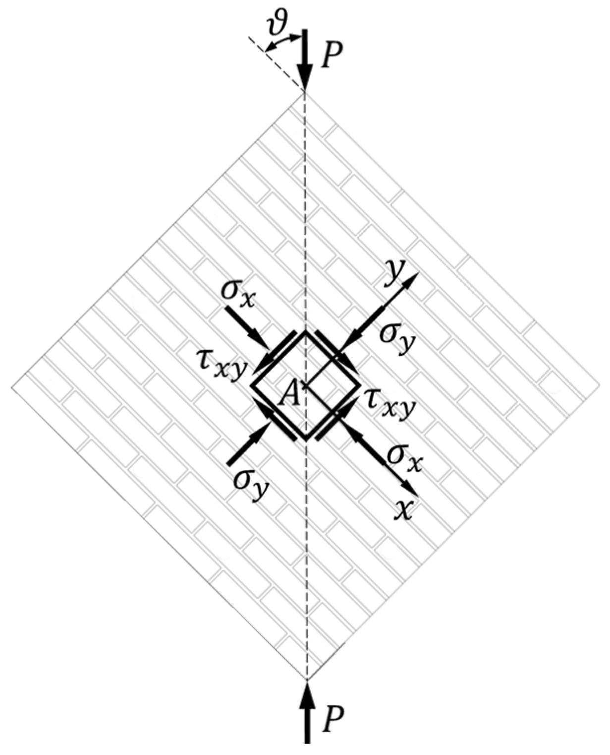
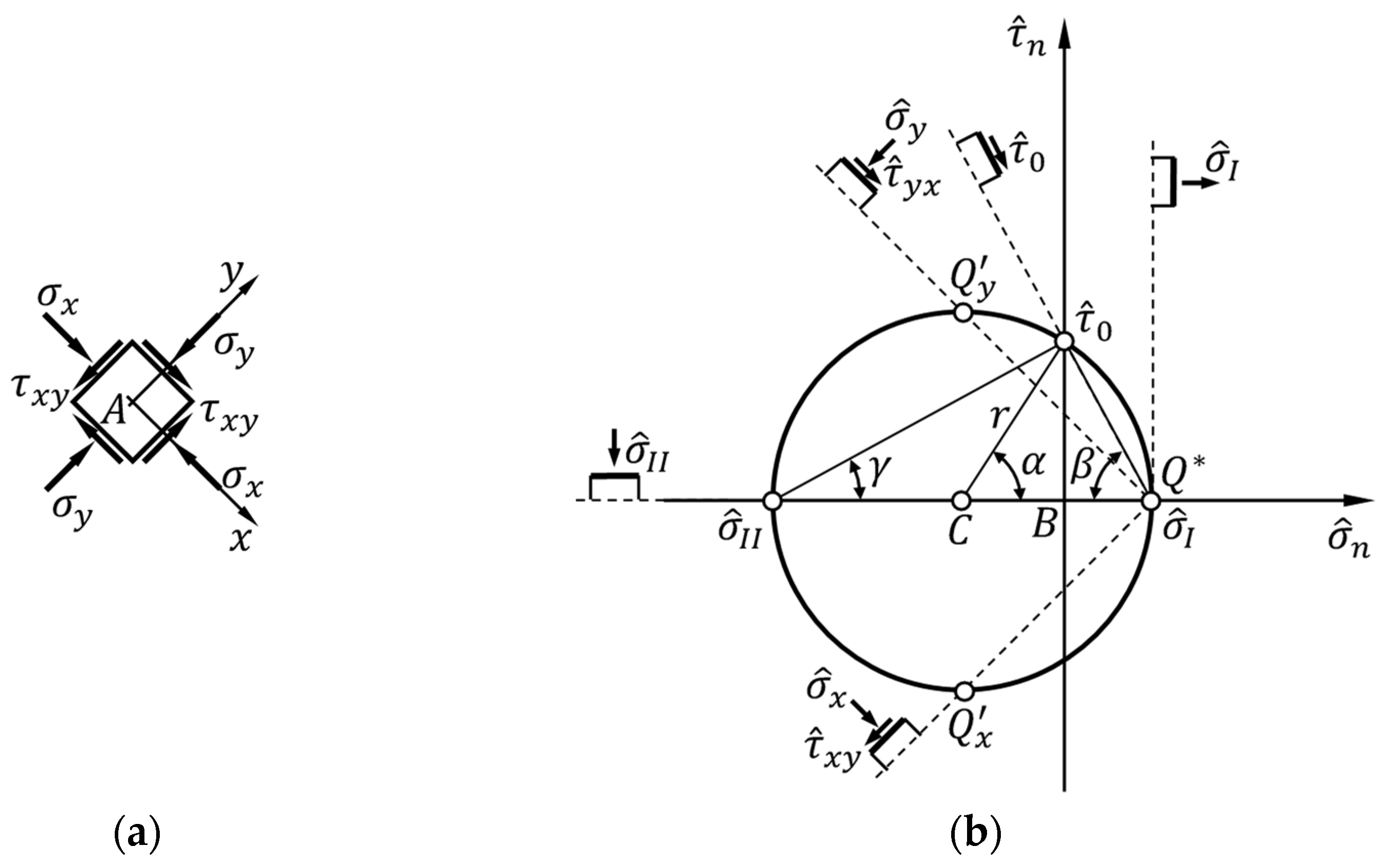
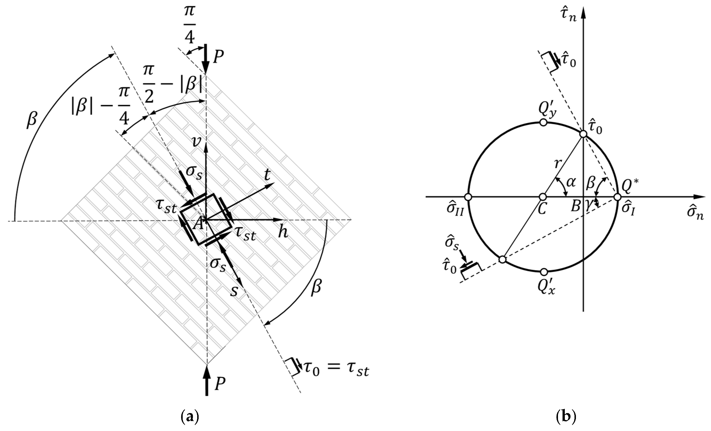
For the stress state and reference frame of Figure 1, also drawn in Figure 3a for convenience, the Pole Method leads to identifying the Mohr pole, $Q^{\ast }$, at the coordinate point $\left({\widehat{\sigma }}_I,0\right)$ of Figure 3b. This is a direct consequence of the Mohr pole property for the stress state, which constitutes the statement of Theorem 1.

Theorem 1. 

The Mohr pole is the only point of the Mohr circle such that the point of intersection of the Mohr circle with a straight line drawn from the Mohr pole with any inclination angle, $\phi$, with respect to the horizontal provides the stress state on the plane inclined at the angle $\phi$ with respect to the horizontal plane [21].

Remembering that the line of intersection of a plane with another plane is the trace of the first plane on the second plane, we can also define the Mohr pole according to the statement of Theorem 2, where the trace is the intersection between a plane parallel to $z$ (the outgoing axis in Figure 3a) and the $x/y$ plane.

Theorem 2. 

The Mohr pole is the only point of the Mohr circle such that the point of intersection of the Mohr circle with a straight line drawn from the Mohr pole with any inclination angle, $\phi$, with respect to the horizontal provides the stress state on the plane whose trace forms an angle of amplitude $\phi$ with respect to the horizontal direction.

Through the condition of parallelism between lines traced by the Mohr pole and traces of the planes on which we want to know the stress components, Theorem 2 establishes a one-to-one relationship between the Mohr pole and the other points of Mohr’s circle. This allows us to find the Mohr pole when we know the coordinates of at least one point on the Mohr circle. To find the Mohr pole, it is therefore sufficient to intersect the Mohr circle with the straight line parallel to the trace of the plane on which the normal stress takes on the value ${{\sigma }_n=\sigma }_x$ and the shear stress takes on the value ${\tau }_n={\tau }_{xy}$ (Figure 3a), plotted from the stress point $Q_x^{\prime }\equiv \left({\widehat{\sigma }}_x,-{\widehat{\tau }}_{xy}\right)$ (Figure 3b). Alternatively, it is possible to intersect the Mohr circle with the straight line parallel to the trace of the plane on which ${{\sigma }_n=\sigma }_y$ and ${\tau }_n={\tau }_{xy}$ (Figure 3a), plotted from the stress point $Q_y^{\prime }\equiv \left({\widehat{\sigma }}_y,{\widehat{\tau }}_{xy}\right)$ (Figure 3b).

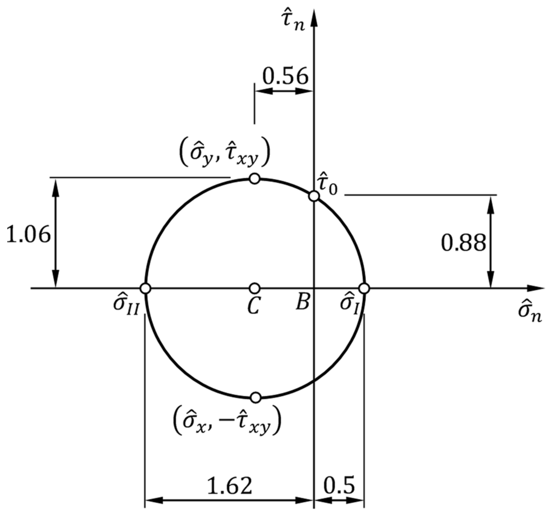
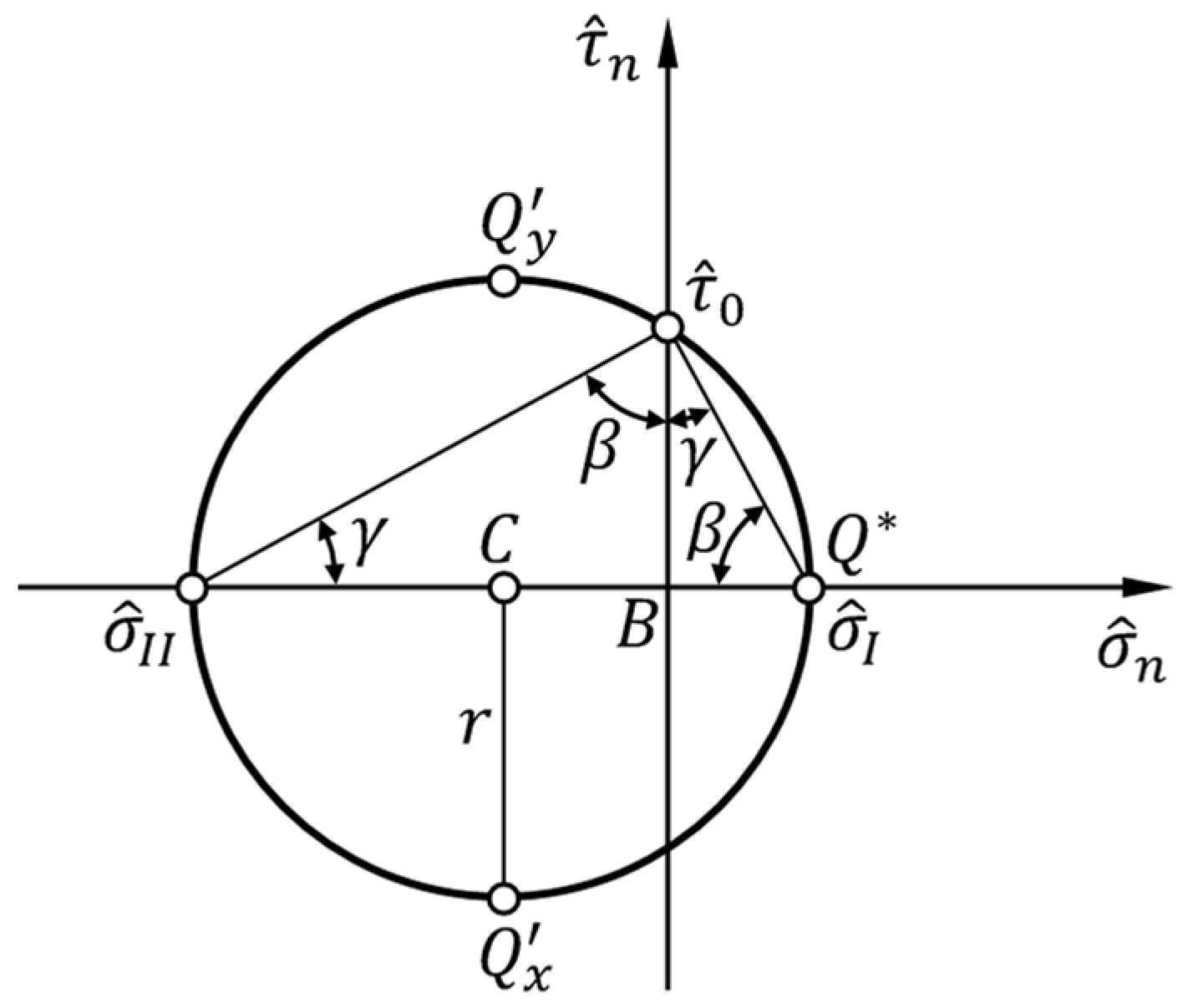
With reference to the symbols introduced in Figure 3b, it is then possible to find a relationship between the two normalized principal stresses and the radius, $r$, of the normalized Mohr circle:

$${\widehat{\sigma }}_I=r-r\mathrm{c}\mathrm{o}\mathrm{s}\left(\alpha \right)=r\left(1-\mathrm{c}\mathrm{o}\mathrm{s}\left(\alpha \right)\right),$$

(18)

$${\widehat{\sigma }}_{II}=-\left(r+r\mathrm{c}\mathrm{o}\mathrm{s}\left(\alpha \right)\right)=-r\left(1+\mathrm{c}\mathrm{o}\mathrm{s}\left(\alpha \right)\right).$$

(19)

The angle $\alpha$ also relates $r$ to ${\widehat{\tau }}_0$, the normalized pure shear stress:

$${\widehat{\tau }}_0=r\mathrm{s}\mathrm{i}\mathrm{n}\left(\alpha \right).$$

(20)

The parameter of the analytical solution proposed in this article is $k$, defined as the ratio between $f_{dc}$ and $f_{dt}$:

$$k=\frac{f_{dc}}{f_{dt}},$$

(21)

which also fixes the ratio (in absolute value) between the two normalized principal stresses:

$$k=\frac{\left|{\widehat{\sigma }}_{II}\right|}{{\widehat{\sigma }}_I},$$

(22)

$${\widehat{\sigma }}_I=\frac{1}{k}\left|{\widehat{\sigma }}_{II}\right|.$$

(23)

By substituting Equations (18) and (19) into Equation (23):

$$r\left(1-\mathrm{c}\mathrm{o}\mathrm{s}\left(\alpha \right)\right)=\frac{1}{k}r\left(1+\mathrm{c}\mathrm{o}\mathrm{s}\left(\alpha \right)\right),$$

(24)

we can therefore express the angle $\alpha$ as a function of the parameter $k$:

$$\alpha =\mathrm{a}\mathrm{r}\mathrm{c}\mathrm{c}\mathrm{o}\mathrm{s}\left(\frac{k-1}{k+1}\right).$$

(25)

Similarly, for the angle $\beta$ in Figure 3b:

$$\beta =\mathrm{a}\mathrm{r}\mathrm{c}\mathrm{t}\mathrm{a}\mathrm{n}\left(\frac{{\widehat{\tau }}_0}{{\widehat{\sigma }}_I}\right)=\mathrm{a}\mathrm{r}\mathrm{c}\mathrm{t}\mathrm{a}\mathrm{n}\left(\frac{\mathrm{s}\mathrm{i}\mathrm{n}\left(\alpha \right)}{1-\mathrm{c}\mathrm{o}\mathrm{s}\left(\alpha \right)}\right),$$

(26)

where we used Equations (18) and (20) to express $\beta$ as a function of $\alpha$. Substituting Equation (25) into Equation (26) then gives the expression of $\beta$ as a function of $k$:

$$\beta =\mathrm{a}\mathrm{r}\mathrm{c}\mathrm{t}\mathrm{a}\mathrm{n}\left(\frac{k+1}{2}\mathrm{s}\mathrm{i}\mathrm{n}\left(\mathrm{a}\mathrm{r}\mathrm{c}\mathrm{c}\mathrm{o}\mathrm{s}\left(\frac{k-1}{k+1}\right)\right)\right).$$

(27)

On the other hand, the relationships established by the angles $\beta$ and $\gamma$ in Figure 3b between the pure shear stress and the principal stresses:

$${\widehat{\tau }}_0={\widehat{\sigma }}_I\mathrm{t}\mathrm{a}\mathrm{n}\left(\beta \right),$$

(28)

$${\widehat{\tau }}_0=-{\widehat{\sigma }}_{II}\mathrm{t}\mathrm{a}\mathrm{n}\left(\gamma \right),$$

(29)

allows us to equate the second terms in Equations (28) and (29):

$$-{\widehat{\sigma }}_{II}\mathrm{t}\mathrm{a}\mathrm{n}\left(\gamma \right)={\widehat{\sigma }}_I\mathrm{t}\mathrm{a}\mathrm{n}\left(\beta \right),$$

(30)

which provides a new expression for the ratio $\left|{\widehat{\sigma }}_{II}\right|/{\widehat{\sigma }}_I$:

$$\frac{\left|{\widehat{\sigma }}_{II}\right|}{{\widehat{\sigma }}_I}=\frac{\mathrm{t}\mathrm{a}\mathrm{n}\left(\beta \right)}{\mathrm{t}\mathrm{a}\mathrm{n}\left(\gamma \right)}.$$

(31)

Moreover, noting that the triangle with vertices at the coordinate points $\left({\widehat{\sigma }}_I,0\right)$, $\left({\widehat{\sigma }}_{II},0\right)$, and $\left(0,{\widehat{\tau }}_0\right)$ is a right-angled triangle—because inscribed in a semicircle (Figure 3b)—$\gamma$ turns out to be the complementary angle of $\beta$:

$$\gamma =\frac{\pi }{2}-\beta .$$

(32)

Therefore, by comparison between Equations (22) and (31), with $\gamma$ expressed by Equation (32):

$$k=\frac{\left|{\widehat{\sigma }}_{II}\right|}{{\widehat{\sigma }}_I}=\frac{\mathrm{t}\mathrm{a}\mathrm{n}\left(\beta \right)}{\mathrm{t}\mathrm{a}\mathrm{n}\left(\frac{\pi }{2}-\beta \right)}={\left(\mathrm{t}\mathrm{a}\mathrm{n}\left(\beta \right)\right)}^2,$$

(33)

which gives a more compact expression of $\beta$ as a function of $k$:

$$\beta =\mathrm{a}\mathrm{r}\mathrm{c}\mathrm{t}\mathrm{a}\mathrm{n}\left(\sqrt{k}\right).$$

(34)

Likewise for the angle $\gamma$:

$$k=\frac{\left|{\widehat{\sigma }}_{II}\right|}{{\widehat{\sigma }}_I}=\frac{\mathrm{t}\mathrm{a}\mathrm{n}\left(\frac{\pi }{2}-\gamma \right)}{\mathrm{t}\mathrm{a}\mathrm{n}\left(\gamma \right)}=\frac{1}{{\left(\mathrm{t}\mathrm{a}\mathrm{n}\left(\gamma \right)\right)}^2},$$

(35)

gives a compact expression of $\gamma$ as a function of $k$:

$$\gamma =\mathrm{a}\mathrm{r}\mathrm{c}\mathrm{t}\mathrm{a}\mathrm{n}\left(\frac{\sqrt{k}}{k}\right).$$

(36)

Finally, noting that $\alpha$ is a central angle subtended by the same arc that subtends the angle at the circumference $\gamma$, we obtain that:

$$\alpha =2\gamma =2\mathrm{a}\mathrm{r}\mathrm{c}\mathrm{t}\mathrm{a}\mathrm{n}\left(\frac{\sqrt{k}}{k}\right),$$

(37)

because the angle subtended by an arc at the center of the circle is double the angle subtended by the same arc at any other point on the circumference of the circle (the central angle theorem).

By expressing the Mohr circle equation in parametric form (in the ${\widehat{\sigma }}_n/{\widehat{\tau }}_n$ plane) using the $\omega$ anomaly:

$${\widehat{\sigma }}_n=\frac{{\widehat{\sigma }}_I+{\widehat{\sigma }}_{II}}{2}+\frac{{\widehat{\sigma }}_I-{\widehat{\sigma }}_{II}}{2}\mathrm{c}\mathrm{o}\mathrm{s}\left(2\omega \right),$$

(38)

$${\widehat{\tau }}_n=\frac{{\widehat{\sigma }}_I-{\widehat{\sigma }}_{II}}{2}\mathrm{s}\mathrm{i}\mathrm{n}\left(2\omega \right),$$

(39)

$\alpha$ is the value of the central angle to assign to the parameter $2\omega$ to reach the coordinate point $\left(0,{\widehat{\tau }}_0\right)$ starting from the coordinate point $\left({\widehat{\sigma }}_I,0\right)$, which represents the stress state on the (vertical) planes (in the neighborhood of $A$) with horizontal normal unit vector:

$${\widehat{\sigma }}_n\left(2\omega =\alpha \right)=\frac{{\widehat{\sigma }}_I+{\widehat{\sigma }}_{II}}{2}+\frac{{\widehat{\sigma }}_I-{\widehat{\sigma }}_{II}}{2}\mathrm{c}\mathrm{o}\mathrm{s}\left(\alpha \right)={\widehat{\sigma }}_x+r\mathrm{c}\mathrm{o}\mathrm{s}\left(\alpha \right)=0,$$

(40)

$${\widehat{\tau }}_n\left(2\omega =\alpha \right)=\frac{{\widehat{\sigma }}_I-{\widehat{\sigma }}_{II}}{2}\mathrm{s}\mathrm{i}\mathrm{n}\left(\alpha \right)=r\mathrm{s}\mathrm{i}\mathrm{n}\left(\alpha \right)={\widehat{\tau }}_0,$$

(41)

where $\alpha$ is a positive angle if it represents a counterclockwise rotation starting from the coordinate point $\left({\widehat{\sigma }}_I,0\right)$. Due to the relationship between the angles $\alpha$ and $\gamma$ (Equation (37)), we can also write:

$${\widehat{\sigma }}_n\left(\omega =\gamma \right)=0,$$

(42)

$${\widehat{\tau }}_n\left(\omega =\gamma \right)={\widehat{\tau }}_0.$$

(43)

The value $\omega =0$ is associated with the vertical trace (in the neighborhood of $A$), which represents the reference trace in the parametric study of the stress state starting from the principal stress values.

Having fixed the ratio between the coordinates of the diametrically opposite points $\left({\widehat{\sigma }}_{II},0\right)$ and $\left({\widehat{\sigma }}_I,0\right)$, to find $r$ and draw the Mohr circle it is sufficient to know the coordinates of at least one point on the Mohr circle. Therefore, it is necessary to relate at least one point of the Mohr circle to the applied load, $P$, in Figure 1.

By the statement of Theorem 2 (for further details see Reference [10]), a pure shear stress, ${\pm \tau }_0$, acts on the planes in the neighborhood of point $A$ whose traces form angles of amplitude $\beta \lessgtr 0$ with the horizontal direction in the $x/y$ plane (Figure 4):

$${\tau }_0=\frac{\left|P\right|}{A_n}{\widehat{\tau }}_0.$$

(44)

For reasons of clarity of representation, Figure 3b shows only the straight line parallel to the trace rotated clockwise ($\beta <0$) with respect to the horizontal direction, which is the same trace in Figure 4, with positive pure shear stress (${+\tau }_0$). However, the property of the Mohr pole identifies a second plane with pure shear stress (${-\tau }_0$) on the Mohr circle, rotated counterclockwise ($\beta >0$) with respect to the horizontal direction. The trace of this second plane in the $x/y$ plane is parallel to the straight line joining the Mohr pole to the coordinate point $\left(0,-{\widehat{\tau }}_0\right)$, not shown in Figure 3b.

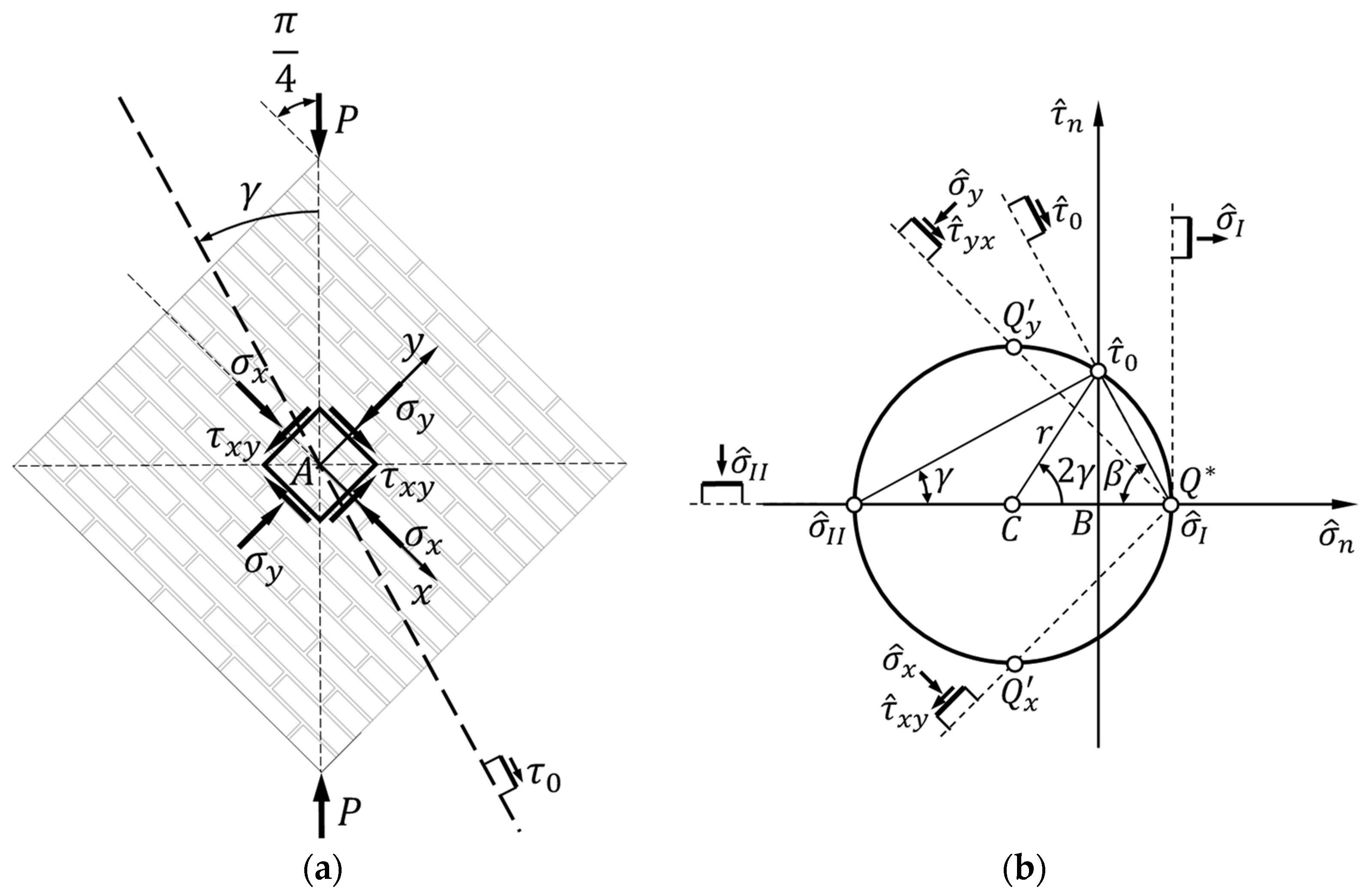
Since the reference trace is vertical, the rotation of the trace with positive pure shear stress,${+\tau }_0$, is the angle $\pi /2-\beta$ in Figure 4, formed with the vertical diagonal. Using Equation (32), the rotation angle $\gamma$—counterclockwise, therefore positive—then identifies the position of the trace with positive pure shear stress (Figure 5a). Since the anomaly of the parametric Mohr circle equations (Equations (38) and (39)) is $2\omega$, $\gamma$ is half the rotation at the center of the Mohr circle needed to reach the coordinate point $\left(0,{\widehat{\tau }}_0\right)$, starting from the coordinate point $\left({\widehat{\sigma }}_I,0\right)$ (Figure 5b). Moreover, the two rotation angles in the reference frame of Figure 5a and in the Mohr circle for the stress state (Figure 5b) have the same direction of rotation.

The ASTM standard [9] decomposes $P$ along the direction of the presumed pure shear stress (the mortar bed joints) and its orthogonal direction (the mortar head joints). Similarly to what the ASTM standard does, we will therefore indicate by $P_s$ the component of $P$ along the traces (in the $x/y$ plane) that form angles of amplitude $\pm \beta$ with the horizontal direction.

Since the standards specify that the specimens for the diagonal compression test must have a square shape [9,12] (Figure 4):

$$\vartheta =\frac{\pi }{4},$$

(45)

$$P_s=\left|P\right|\mathrm{c}\mathrm{o}\mathrm{s}\left(\frac{\pi }{2}-\beta \right).$$

(46)

The area of the wallette intersected by a plane inclined at an angle $\beta$ (Figure 4) is:

$$A_{ns}=\frac{A_n}{\mathrm{c}\mathrm{o}\mathrm{s}\left(\beta -\frac{\pi }{4}\right)}.$$

(47)

The pure shear stress (in absolute value) on the planes inclined at angles $\pm \beta$ is therefore:

$${\tau }_0=\frac{P_s}{A_{ns}}=\frac{\left|P\right|}{A_n}\mathrm{s}\mathrm{i}\mathrm{n}\left(\beta \right)\mathrm{c}\mathrm{o}\mathrm{s}\left(\beta -\frac{\pi }{4}\right),$$

(48)

which provides the normalized pure shear stress on the planes inclined at angles $\pm \beta$, as a function of $\beta$:

$${\widehat{\tau }}_0=\frac{A_n}{\left|P\right|}{\tau }_0=\mathrm{s}\mathrm{i}\mathrm{n}\left(\beta \right)\mathrm{c}\mathrm{o}\mathrm{s}\left(\beta -\frac{\pi }{4}\right).$$

(49)

After substituting Equation (34) into Equation (49), the expression of ${\widehat{\tau }}_0$ as a function of the parameter $k$ is:

$${\widehat{\tau }}_0=\mathrm{s}\mathrm{i}\mathrm{n}\left(\mathrm{a}\mathrm{r}\mathrm{c}\mathrm{t}\mathrm{a}\mathrm{n}\left(\sqrt{k}\right)\right)\mathrm{c}\mathrm{o}\mathrm{s}\left(\mathrm{a}\mathrm{r}\mathrm{c}\mathrm{t}\mathrm{a}\mathrm{n}\left(\sqrt{k}\right)-\frac{\pi }{4}\right).$$

(50)

Remembering the trigonometric relationships between $\mathrm{s}\mathrm{i}\mathrm{n}\left(\phi \right)$ and $\mathrm{t}\mathrm{a}\mathrm{n}\left(\phi \right)$ and between $\mathrm{c}\mathrm{o}\mathrm{s}\left(\phi \right)$ and $\mathrm{t}\mathrm{a}\mathrm{n}\left(\phi \right)$ (derived from the defining relation for $\mathrm{t}\mathrm{a}\mathrm{n}\left(\phi \right)$ and the Pythagorean formula for sines and cosines):

$$\mathrm{s}\mathrm{i}\mathrm{n}\left(\phi \right)=\pm \frac{\mathrm{t}\mathrm{a}\mathrm{n}\left(\phi \right)}{\sqrt{1+{\mathrm{t}\mathrm{a}\mathrm{n}}^2\left(\phi \right)}},$$

(51)

$$\mathrm{c}\mathrm{o}\mathrm{s}\left(\phi \right)=\pm \frac{1}{\sqrt{1+{\mathrm{t}\mathrm{a}\mathrm{n}}^2\left(\phi \right)}},$$

(52)

and using Ptolemy’s identity that gives the difference formula for cosine:

$$\mathrm{c}\mathrm{o}\mathrm{s}\left(\phi -\theta \right)=\mathrm{c}\mathrm{o}\mathrm{s}\left(\phi \right)\mathrm{c}\mathrm{o}\mathrm{s}\left(\theta \right)+\mathrm{s}\mathrm{i}\mathrm{n}\left(\phi \right)\mathrm{s}\mathrm{i}\mathrm{n}\left(\theta \right).$$

(53)

we can rewrite Equation (50) in the form:

$${\widehat{\tau }}_0=\frac{\sqrt{2}}{2}\frac{\sqrt{k}\left(1+\sqrt{k}\right)}{1+k},$$

(54)

where we chose the positive sign for $\mathrm{s}\mathrm{i}\mathrm{n}\left(\beta \right)$, with $\beta =\mathrm{a}\mathrm{r}\mathrm{c}\mathrm{t}\mathrm{a}\mathrm{n}\left(\sqrt{k}\right)$, because $\beta$ is a positive scalar in Figure 4 (as in Figure 3b), not the value of an oriented angle. Moreover, since:

$$0\le \beta \le \frac{\pi }{2},$$

(55)

the sign of $\mathrm{c}\mathrm{o}\mathrm{s}\left(\beta \right)$ is also positive.

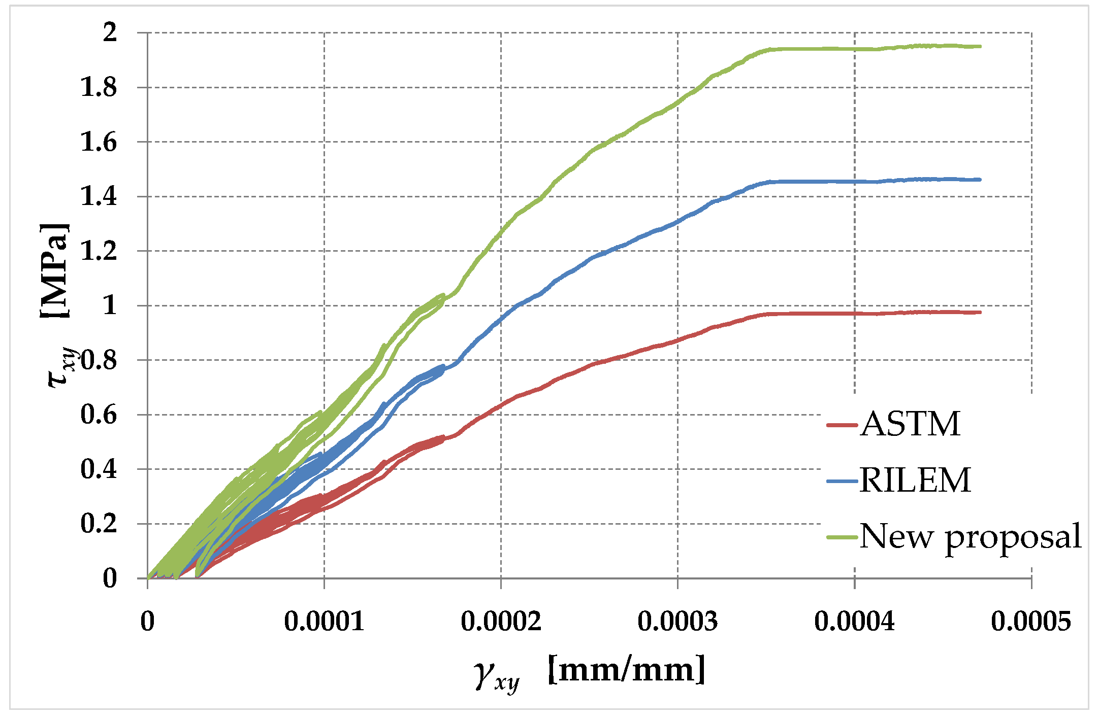
Equation (54) allows a direct comparison between the value that ${\widehat{\tau }}_0$ takes in the new proposal and ${\widehat{\tau }}_0^{ASTM}$, the normalized pure shear stress in the ASTM interpretation of the diagonal compression test:

$${\widehat{\tau }}_0^{ASTM}=\frac{\sqrt{2}}{2}.$$

(56)

In fact, by recognizing the value of ${\widehat{\tau }}_0^{ASTM}$ in the multiplicative factor of Equation (54), we can define $c_{{\tau }_0}$:

$$c_{{\tau }_0}=\sqrt{k}\frac{1+\sqrt{k}}{1+k},$$

(57)

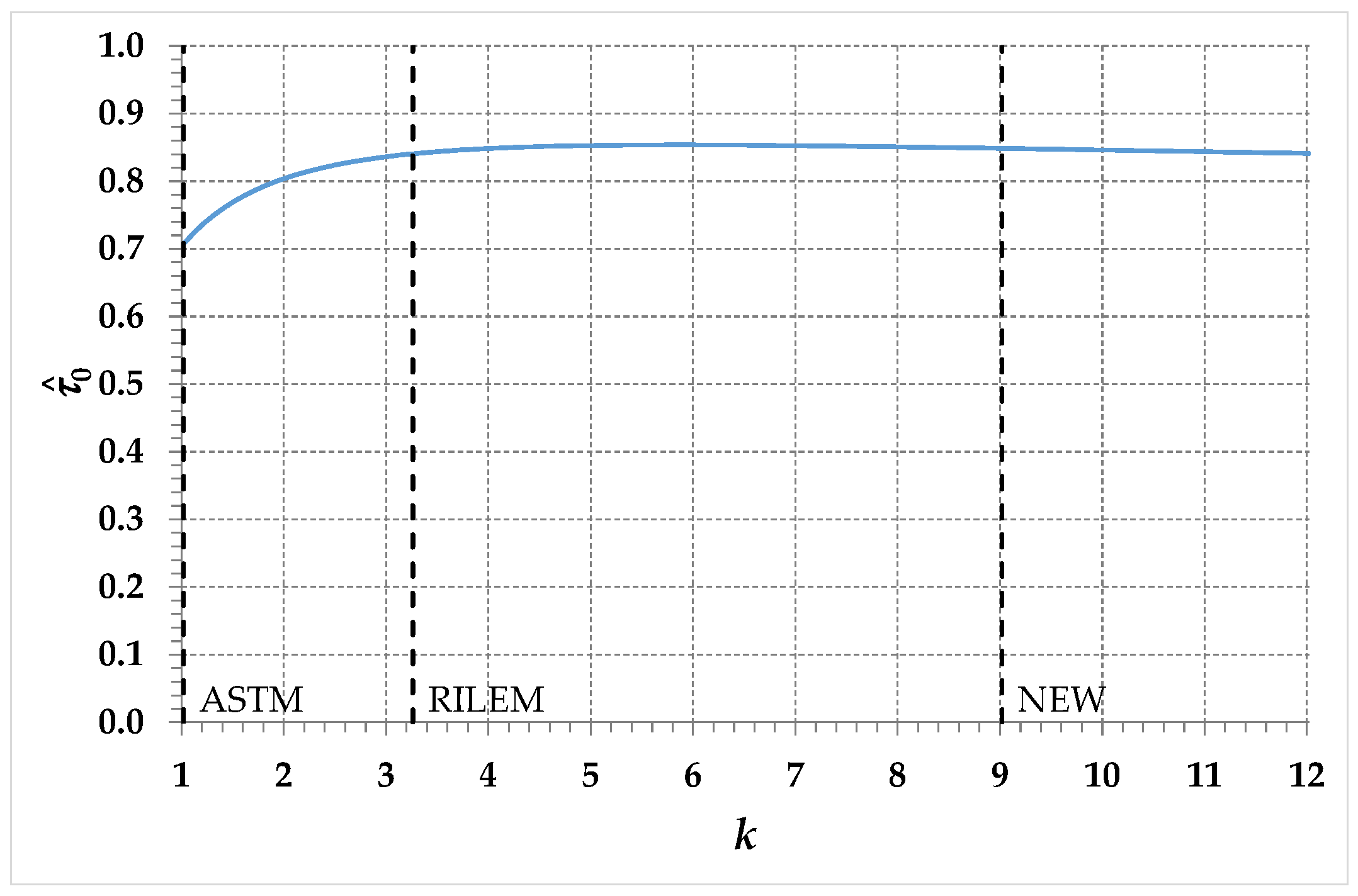
as the correction factor of the normalized pure shear stress, with respect to the ASTM interpretation of the diagonal compression test:

$${\widehat{\tau }}_0=c_{{\tau }_0}{\tau }_0^{ASTM}.$$

(58)

Since the right-angled triangle with vertices at the coordinate points $\left({\widehat{\sigma }}_I,0\right)$, $\left(\mathrm{0,0}\right)$, and $\left(0,{\widehat{\tau }}_0\right)$ is similar to the right-angled triangle with vertices at the coordinate points $\left(\mathrm{0,0}\right)$, $\left({\widehat{\sigma }}_{II},0\right)$, and $\left(0,{\widehat{\tau }}_0\right)$ (Figure 6), ${\widehat{\sigma }}_I$ and ${\widehat{\sigma }}_{II}$ are directly proportional to ${\widehat{\tau }}_0$ through the tangents of the angles $\gamma$ and $\beta$, respectively:

$$\begin{array}{cc}\hfill {\widehat{\sigma }}_I={\widehat{\tau }}_0\mathrm{t}\mathrm{a}\mathrm{n}\left(\gamma \right)& =\frac{\sqrt{k}}{k}{\widehat{\tau }}_0=\frac{\sqrt{k}}{k}\mathrm{s}\mathrm{i}\mathrm{n}\left(\mathrm{a}\mathrm{r}\mathrm{c}\mathrm{t}\mathrm{a}\mathrm{n}\left(\sqrt{k}\right)\right)\mathrm{c}\mathrm{o}\mathrm{s}\left(\mathrm{a}\mathrm{r}\mathrm{c}\mathrm{t}\mathrm{a}\mathrm{n}\left(\sqrt{k}\right)-\frac{\pi }{4}\right)\hfill \\ & =\frac{\sqrt{2}}{2}\frac{1+\sqrt{k}}{1+k},\hfill \end{array}$$

(59)

$$\begin{array}{cc}\hfill {\widehat{\sigma }}_{II}=-{\widehat{\tau }}_0\mathrm{t}\mathrm{a}\mathrm{n}\left(\beta \right)& =-\sqrt{k}{\widehat{\tau }}_0=-\sqrt{k}\mathrm{s}\mathrm{i}\mathrm{n}\left(\mathrm{a}\mathrm{r}\mathrm{c}\mathrm{t}\mathrm{a}\mathrm{n}\left(\sqrt{k}\right)\right)\mathrm{c}\mathrm{o}\mathrm{s}\left(\mathrm{a}\mathrm{r}\mathrm{c}\mathrm{t}\mathrm{a}\mathrm{n}\left(\sqrt{k}\right)-\frac{\pi }{4}\right)\hfill \\ & =-\frac{\sqrt{2}}{2}k\frac{1+\sqrt{k}}{1+k},\hfill \end{array}$$

(60)

where we made use of Equations (34) and (36).

The half-sum between ${\widehat{\sigma }}_I$ and ${\widehat{\sigma }}_{II}$ then gives the first coordinate of the center of the circle, $C$, which is equal to the first coordinates of the points $Q_x^{\prime }$ and $Q_y^{\prime }$ (Figure 6):

$$\begin{array}{cc}\hfill {\widehat{\sigma }}_x={\widehat{\sigma }}_y& =\frac{{\widehat{\sigma }}_I+{\widehat{\sigma }}_{II}}{2}=\frac{1-k}{2k}\sqrt{k}{\widehat{\tau }}_0\hfill \\ & =\frac{1-k}{2k}\sqrt{k}\mathrm{s}\mathrm{i}\mathrm{n}\left(\mathrm{a}\mathrm{r}\mathrm{c}\mathrm{t}\mathrm{a}\mathrm{n}\left(\sqrt{k}\right)\right)\mathrm{c}\mathrm{o}\mathrm{s}\left(\mathrm{a}\mathrm{r}\mathrm{c}\mathrm{t}\mathrm{a}\mathrm{n}\left(\sqrt{k}\right)-\frac{\pi }{4}\right)\hfill \\ & =\frac{\sqrt{2}}{4}\left(1+\sqrt{k}\right)\frac{1-k}{1+k},\hfill \end{array}$$

(61)

while the half-difference between ${\widehat{\sigma }}_I$ and ${\widehat{\sigma }}_{II}$ provides the radius, $r$, which is equal to the second coordinates (in absolute value) of the points $Q_x^{\prime }$ and $Q_y^{\prime }$ (Figure 6):

$$\begin{array}{cc}\hfill {\widehat{\tau }}_{xy}=r=\frac{{\widehat{\sigma }}_I-{\widehat{\sigma }}_{II}}{2}& =\frac{1+k}{2k}\sqrt{k}{\widehat{\tau }}_0\hfill \\ & =\frac{1+k}{2k}\sqrt{k}\mathrm{s}\mathrm{i}\mathrm{n}\left(\mathrm{a}\mathrm{r}\mathrm{c}\mathrm{t}\mathrm{a}\mathrm{n}\left(\sqrt{k}\right)\right)\mathrm{c}\mathrm{o}\mathrm{s}\left(\mathrm{a}\mathrm{r}\mathrm{c}\mathrm{t}\mathrm{a}\mathrm{n}\left(\sqrt{k}\right)-\frac{\pi }{4}\right)\hfill \\ & =\frac{\sqrt{2}}{4}\left(1+\sqrt{k}\right).\hfill \end{array}$$

(62)

Equations (61) and (62) therefore replace the normalizations of Equations (4)–(6). Having expressed the solution of the new formulation as a function of a single parameter, $k$, the knowledge of $k$ directly provides the stress state at point $A$. Seen in these terms, the coefficient $k$ becomes an unknown of the problem of determining the stress state at point $A$. To find $k$, it is necessary to couple Equations (61) and (62) with an additional condition (Section 4).

As a further observation, the comparison between Equations (20) and (62) provides an expression of the angle $\alpha$ as a function of both $k$ and $\sqrt{k}$:

$$\alpha =\mathrm{a}\mathrm{r}\mathrm{c}\mathrm{s}\mathrm{i}\mathrm{n}\left(\frac{2\sqrt{k}}{1+k}\right).$$

(63)

3.2. Strain State at Point $A$

As known, strain analysis deals with the study of continuum deformation, which is a geometric problem and has nothing to do with the properties of materials. The description of the deformation therefore requires the introduction of some geometric quantities and algebraic operators [22].

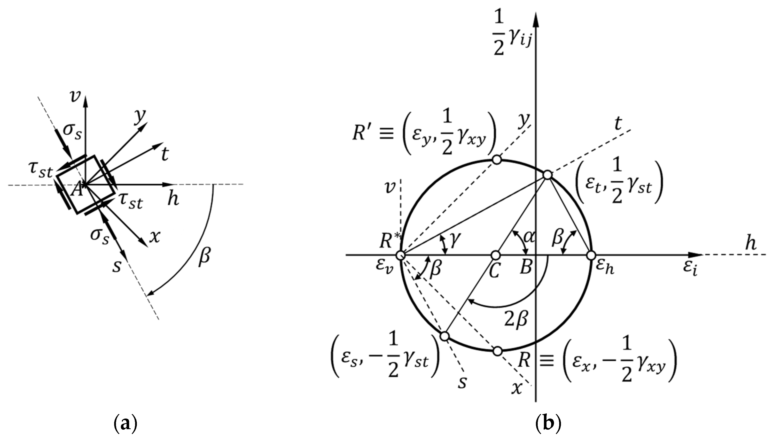
Denoted as $h$ and $v$, respectively, the horizontal and vertical axes of the reference system of origin $A$ (Figure 7a), let $\left[\epsilon \right]$ be the infinitesimal strain tensor in the neighborhood of point $A$ (infinitesimal strain theory):

$$\left[\epsilon \right]=\left[\begin{array}{ccc}{\epsilon }_h& \frac{1}{2}{\gamma }_{hv}& \frac{1}{2}{\gamma }_{hz}\\ \frac{1}{2}{\gamma }_{hv}& {\epsilon }_v& \frac{1}{2}{\gamma }_{vz}\\ \frac{1}{2}{\gamma }_{hz}& \frac{1}{2}{\gamma }_{vz}& {\epsilon }_z\end{array}\right],$$

(64)

where $z$ indicates the direction orthogonal to the $h/v$ plane.

It is worth noting that $\beta$ is no longer a positive scalar in Figure 7a, because it is the amplitude of an oriented angle, which indicates the angle of rotation of the positive $s$ half-axis relative to the positive $h$ half-axis. Since positive values of an angle of rotation correspond to counterclockwise rotations, $\beta$ is a negative rotation angle in Figure 7a.

The positive $s$ half-axis lies on the trace of one of the two planes of pure shear stress, ${\tau }_0$ (Figure 7b). Therefore, there are no normal stresses on the planes (in the neighborhood of $A$) parallel to $s$ (Figure 7a):

$${\sigma }_t=0.$$

(65)

On the planes perpendicular to $s$, however, both normal and shear stresses are present, ${\sigma }_s$ and ${\tau }_{st}={\tau }_0$, respectively (Figure 7a). In fact, a straight line drawn from the Mohr pole, $Q^{*}$, in a direction perpendicular to the $s$-axis (the line that forms an angle of amplitude $\gamma$ with the horizontal direction in Figure 7b) intersects the Mohr circle at a point with first coordinate ${\sigma }_s<0$ (Figure 7b). This means that the stress state at point $A$ is the sum of a pure shear stress and a uniaxial compressive stress state in the $s$-axis direction.

In linear elasticity, the principal directions of stress coincide with the principal direction of strain. This cancels out the change in the angles between the axes $h$, $v$, and $z$, since $h$ and $v$ lie along the principal directions of stress found in Section 3.1 ($z$ is one of the principal directions of stress as a result of the stress state at point $A$, which is a plane stress state):

$${\gamma }_{hv}={\gamma }_{hz}={\gamma }_{vz}=0,$$

(66)

$$\left[\epsilon \right]=\left[\begin{array}{ccc}{\epsilon }_h& 0& 0\\ 0& {\epsilon }_v& 0\\ 0& 0& {\epsilon }_z\end{array}\right].$$

(67)

The transformation of the strain components from the reference system $(A,h,v,z)$ to the reference system $(A,s,t,z)$ respects the typical transformation law of double symmetric tensors:

$$\left[\begin{array}{ccc}{\epsilon }_s& \frac{1}{2}{\gamma }_{st}& \frac{1}{2}{\gamma }_{sz}\\ \frac{1}{2}{\gamma }_{st}& {\epsilon }_t& \frac{1}{2}{\gamma }_{tz}\\ \frac{1}{2}{\gamma }_{sz}& \frac{1}{2}{\gamma }_{tz}& {\epsilon }_z\end{array}\right]=\left[\begin{array}{ccc}{a}_h& a_v& a_z\\ b_h& b_v& b_z\\ c_h& c_v& c_z\end{array}\right]\left[\begin{array}{ccc}{\epsilon }_h& 0& 0\\ 0& {\epsilon }_v& 0\\ 0& 0& {\epsilon }_z\end{array}\right]\left[\begin{array}{ccc}{a}_h& b_h& c_h\\ a_v& b_v& c_v\\ a_z& b_z& c_z\end{array}\right],$$

(68)

where $a_h$, $a_v$, $a_z$, $b_h$, $b_v$, $b_z$, $c_h$, $c_v$, and $c_z$ are the direction cosines of the three positive coordinate axes $s$, $t$, and $z$ with respect to the three positive coordinate axes $h$, $v$, and $z$ (Appendix A).

The transformation law therefore reads:

$$\left[\begin{array}{ccc}{\epsilon }_s& \frac{1}{2}{\gamma }_{st}& \frac{1}{2}{\gamma }_{sz}\\ \frac{1}{2}{\gamma }_{st}& {\epsilon }_t& \frac{1}{2}{\gamma }_{tz}\\ \frac{1}{2}{\gamma }_{sz}& \frac{1}{2}{\gamma }_{tz}& {\epsilon }_z\end{array}\right]=\left[\begin{array}{ccc}\mathrm{c}\mathrm{o}\mathrm{s}\left(\beta \right)& \mathrm{s}\mathrm{i}\mathrm{n}\left(\beta \right)& 0\\ -\mathrm{s}\mathrm{i}\mathrm{n}\left(\beta \right)& \mathrm{c}\mathrm{o}\mathrm{s}\left(\beta \right)& 0\\ 0& 0& 1\end{array}\right]\left[\begin{array}{ccc}{\epsilon }_h& 0& 0\\ 0& {\epsilon }_v& 0\\ 0& 0& {\epsilon }_z\end{array}\right]\left[\begin{array}{ccc}\mathrm{c}\mathrm{o}\mathrm{s}\left(\beta \right)& -\mathrm{s}\mathrm{i}\mathrm{n}\left(\beta \right)& 0\\ \mathrm{s}\mathrm{i}\mathrm{n}\left(\beta \right)& \mathrm{c}\mathrm{o}\mathrm{s}\left(\beta \right)& 0\\ 0& 0& 1\end{array}\right].$$

(69)

From Equations (68) and (69), it follows that the normal strain along the $s$-axis direction is a quadratic form of the direction cosines:

$${\epsilon }_s={\epsilon }_h{a}_h^2+{\epsilon }_v{a}_v^2={\epsilon }_h{\mathrm{c}\mathrm{o}\mathrm{s}}^2\left(\beta \right)+{\epsilon }_v{\mathrm{s}\mathrm{i}\mathrm{n}}^2\left(\beta \right).$$

(70)

Since from Equations (51) and (52) it follows that:

$${\mathrm{c}\mathrm{o}\mathrm{s}}^2\left(\beta \right)=\frac{1}{1+{\mathrm{t}\mathrm{a}\mathrm{n}}^2\left(\beta \right)}=\frac{1}{1+k},$$

(71)

$${\mathrm{s}\mathrm{i}\mathrm{n}}^2\left(\beta \right)=\frac{{\mathrm{t}\mathrm{a}\mathrm{n}}^2\left(\beta \right)}{1+{\mathrm{t}\mathrm{a}\mathrm{n}}^2\left(\beta \right)}=\frac{k}{1+k},$$

(72)

where we made use of Equation (34), ${\epsilon }_s$ also reads:

$${\epsilon }_s=\frac{1}{1+k}\left({\epsilon }_h+{k\epsilon }_v\right).$$

(73)

The Double-Angle Formulas then allow us to write the terms ${\mathrm{c}\mathrm{o}\mathrm{s}}^2\left(\beta \right)$ and ${\mathrm{s}\mathrm{i}\mathrm{n}}^2\left(\beta \right)$ in Equation (70) as functions of $\mathrm{c}\mathrm{o}\mathrm{s}\left(2\beta \right)$:

$${\mathrm{c}\mathrm{o}\mathrm{s}}^2\left(\beta \right)=\frac{1+\mathrm{c}\mathrm{o}\mathrm{s}\left(2\beta \right)}{2},$$

(74)

$${\mathrm{s}\mathrm{i}\mathrm{n}}^2\left(\beta \right)=\frac{1-\mathrm{c}\mathrm{o}\mathrm{s}\left(2\beta \right)}{2},$$

(75)

which gives the expression of ${\epsilon }_s$ as a function of the angle $2\beta$, after substituting Equations (74) and (75) into Equation (70):

$${\epsilon }_s=\frac{{\epsilon }_h+{\epsilon }_v}{2}+\frac{{\epsilon }_h-{\epsilon }_v}{2}\mathrm{c}\mathrm{o}\mathrm{s}\left(2\beta \right).$$

(76)

Similarly for the normal strain along the $t$-axis direction:

$${\epsilon }_t={\epsilon }_h{b}_h^2+{\epsilon }_v{b}_v^2={\epsilon }_h{\mathrm{s}\mathrm{i}\mathrm{n}}^2\left(\beta \right)+{\epsilon }_v{\mathrm{c}\mathrm{o}\mathrm{s}}^2\left(\beta \right),$$

(77)

we can find the relationship between ${\epsilon }_t$ and $k$:

$${\epsilon }_t={\epsilon }_h\frac{{\mathrm{t}\mathrm{a}\mathrm{n}}^2\left(\beta \right)}{1+{\mathrm{t}\mathrm{a}\mathrm{n}}^2\left(\beta \right)}+{\epsilon }_v\frac{1}{1+{\mathrm{t}\mathrm{a}\mathrm{n}}^2\left(\beta \right)}=\frac{1}{1+k}\left(k{\epsilon }_h+{\epsilon }_v\right),$$

(78)

while the Double-Angle Formulas provide the expression of ${\epsilon }_t$ in function of the angle $2\beta$:

$${\epsilon }_t=\frac{{\epsilon }_h+{\epsilon }_v}{2}-\frac{{\epsilon }_h-{\epsilon }_v}{2}\mathrm{c}\mathrm{o}\mathrm{s}\left(2\beta \right).$$

(79)

The shear strain ${\gamma }_{st}$ is defined as positive if it causes the right angle of the first quadrant (between the $+s$ and $+t$-axes) to decrease. Its expression, given by Equation (68), is a bilinear form of the direction cosines:

$$\frac{1}{2}{\gamma }_{st}={\epsilon }_h{a}_h{b}_h+{\epsilon }_v{a}_v{b}_v=-{\epsilon }_h\mathrm{c}\mathrm{o}\mathrm{s}\left(\beta \right)\mathrm{s}\mathrm{i}\mathrm{n}\left(\beta \right)+{\epsilon }_v\mathrm{s}\mathrm{i}\mathrm{n}\left(\beta \right)\mathrm{c}\mathrm{o}\mathrm{s}\left(\beta \right).$$

(80)

By rewriting Equation (80) in the form:

$$\frac{1}{2}{\gamma }_{st}=-2\frac{{\epsilon }_h-{\epsilon }_v}{2}\mathrm{s}\mathrm{i}\mathrm{n}\left(\beta \right)\mathrm{c}\mathrm{o}\mathrm{s}\left(\beta \right),$$

(81)

and recognizing the sine of the angle $2\beta$ in the double product $2\mathrm{s}\mathrm{i}\mathrm{n}\left(\beta \right)\mathrm{c}\mathrm{o}\mathrm{s}\left(\beta \right)$:

$$2\mathrm{s}\mathrm{i}\mathrm{n}\left(\beta \right)\mathrm{c}\mathrm{o}\mathrm{s}\left(\beta \right)=\mathrm{s}\mathrm{i}\mathrm{n}\left(2\beta \right),$$

(82)

we finally obtain:

$$\frac{1}{2}{\gamma }_{st}=-\frac{{\epsilon }_h-{\epsilon }_v}{2}\mathrm{s}\mathrm{i}\mathrm{n}\left(2\beta \right).$$

(83)

In the assumption of a generic rotation angle, $\delta$, between the two reference systems of Figure 7a (redrawn, for convenience, in Figure 8a), the functions of the angle $2\beta$ provided by Equations (76) and (83) allow a parametric plot in the parameter $2\delta$ of the strain state at point $A$, in the plane defined by the axes ${\epsilon }_i$ and ${1/2\gamma }_{ij}$:

$${\epsilon }_i=\frac{{\epsilon }_h+{\epsilon }_v}{2}+\frac{{\epsilon }_h-{\epsilon }_v}{2}\mathrm{c}\mathrm{o}\mathrm{s}\left(2\delta \right),$$

(84)

$$\frac{1}{2}{\gamma }_{ij}=-\frac{{\epsilon }_h-{\epsilon }_v}{2}\mathrm{s}\mathrm{i}\mathrm{n}\left(2\delta \right).$$

(85)

As with the stress state (Equations (38) and (39)), the parametric plot of the strain state at point $A$ is a circle centered on the horizontal axis (Figure 8b). By analogy with the stress state, we can denote this graph as the Mohr circle for the strain state and the plane of the graph as the Mohr plane for the strain state. The center of the Mohr circle for the strain state is point $C$, as for the stress state.

Equations (84) and (85) allow us to reach the coordinate point $\left({\epsilon }_s,-1/2{\gamma }_{st}\right)$ after a rotation at the center, $C$, equal to $2\beta$, starting from the coordinate point $\left({\epsilon }_h,0\right)$ (Figure 8b):

$${\epsilon }_i\left(\delta =\beta \right)=\frac{{\epsilon }_h+{\epsilon }_v}{2}+\frac{{\epsilon }_h-{\epsilon }_v}{2}\mathrm{c}\mathrm{o}\mathrm{s}\left(2\beta \right)={\epsilon }_s,$$

(86)

$$\frac{1}{2}{\gamma }_{ij}\left(\delta =\beta \right)=-\frac{{\epsilon }_h-{\epsilon }_v}{2}\mathrm{s}\mathrm{i}\mathrm{n}\left(2\beta \right)=\frac{1}{2}{\gamma }_{st}.$$

(87)

Since ${\epsilon }_h>0$ and ${\epsilon }_v<0$, it follows from Equation (87) that ${\gamma }_{st}>0$ for $\beta <0$ (clockwise rotation, as in Figure 8a) and ${\gamma }_{st}<0$ for $\beta >0$ (counterclockwise rotation). Consequently, after a rotation at the center, $C$, equal to $-\pi /2$ (the angle that is double the clockwise rotation, around point $A$, which causes the $h$-axis to overlap with the $x$-axis), we reach the coordinate point $\left({\epsilon }_x,-1/2{\gamma }_{xy}\right)$, with ${\gamma }_{xy}>0$ (Figure 8b):

$$\frac{1}{2}{\gamma }_{xy}=\frac{1}{2}{\gamma }_{ij}\left(\delta =-\frac{\pi }{4}\right)=\frac{{\epsilon }_h-{\epsilon }_v}{2},$$

(88)

which is the same expression provided by the ASTM guidelines and adopted by all other standards.

Due to the presence of a uniaxial compressive stress state in the $s$-axis direction (the normal stress ${\sigma }_s$ in Figure 8a), the normal strain in the $t$-axis direction is positive, because of the Poisson effect:

$${\epsilon }_t=-\nu {\epsilon }_s>0,$$

(89)

where $\nu$ is the Poisson ratio. This causes the coordinate point $\left({\epsilon }_t,1/2{\gamma }_{st}\right)$ not to be on the vertical axis of Figure 8b.

Furthermore, the point $R^{*}$ in Figure 8b is the only point on the Mohr circle that enjoys the property stated in Theorem 3.

Theorem 3. 

A straight line drawn from $R^{*}$ in the direction of the $i$-axis intersects the Mohr circle at a point whose coordinates are ${\epsilon }_i$ and $-1/2{\gamma }_{ij}$ where $j$ is the axis rotated by $\pi /2$ in a counterclockwise direction with respect to $i$.

We will denote $R^{*}$ as the Mohr pole of the strain state. Due to the property of $R^{*}$, the coordinate point $\left({\epsilon }_t,1/2{\gamma }_{st}\right)$ lies on the straight line drawn from $R^{*}$ in the direction of the $t$-axis (Figure 8b). Since ${\epsilon }_t>0$, the strain state on planes (in the neighborhood of $A$) perpendicular to $t$ is not a state of pure shear strain, although the stress state on those planes is a state of pure shear stress. Therefore, it is not possible to use the shear strain ${\gamma }_{st}$ together with the shear stress ${\tau }_{st}={\tau }_0$ to plot the shear stress–shear strain curves for masonry.

It is worth noting that the coordinates ${\epsilon }_i$ and $-1/2{\gamma }_{ij}$ in the Mohr plane take on a specific meaning for the point $P$ of the $i$-axis that is at a unit distance from point $A$:

• ${\epsilon }_i=u_i$, where $u_i$ is the displacement component of point $P$ in the direction of the $i$-axis (normal component of the displacement, or normal displacement);
• $1/2{\gamma }_{ij}=u_j$, where $u_j$ is the displacement component of point $P$ in the direction of the $j$-axis (tangential component of the displacement, or tangential displacement).

This justifies the use of the letter $R$ for the points in the Mohr plane for the strain state, as $R$ is the capital letter in the Western alphabet that corresponds to $\rho$, the Greek letter used to denote the displacement vector.

3.3. Elastic Coefficients

Since the elementary cube (in the neighborhood of point $A$) with faces perpendicular to the $s$- and $t$-axes is subjected to both pure shear stress and uniaxial compression in the direction of the $s$-axis (Figure 8a), we can calculate the Young modulus as the ratio of the normal stress ${\sigma }_s$ and the normal strain ${\epsilon }_s$ (linear elastic theory):

$$E=\frac{{\sigma }_s}{{\epsilon }_s}.$$

(90)

In fact, the shear stress does not involve any component of normal strain in homogeneous and isotropic linear elastic materials (pure shear stress and normal stress are decoupled problems), which allows us to calculate $E$ as if the elementary cube were in uniaxial compression. By noting (in Figure 7b) that ${\sigma }_s$ is double the first coordinate of the center, $C$, of the Mohr circle, given by Equation (61):

$${\sigma }_s={\sigma }_I+{\sigma }_{II}=2{\sigma }_x=\frac{\sqrt{2}}{2}\left(1+\sqrt{k}\right)\frac{1-k}{1+k}\frac{\left|P\right|}{A_n},$$

(91)

and using Equation (73) for the value of ${\epsilon }_s$, we obtain:

$$E=\frac{\sqrt{2}}{2}\frac{\left(1+\sqrt{k}\right)\left(1-k\right)}{{\epsilon }_h+{k\epsilon }_v}\frac{\left|P\right|}{A_n}.$$

(92)

Equations (73), (78) and (89) then allow us to find a relationship between the Poisson ratio, $k$, and the principal strains along the diagonals:

$$\nu =-\frac{{\epsilon }_t}{{\epsilon }_s}=-\frac{k{\epsilon }_h+{\epsilon }_v}{{\epsilon }_h+{k\epsilon }_v}.$$

(93)

It is worth noting that we could obtain the result in Equation (92) using Hooke’s laws with ${\sigma }_z=0$ (plane stress state), to find ${\epsilon }_h$ and ${\epsilon }_v$:

$${\epsilon }_h=\frac{1}{E}\left[{\sigma }_I-\nu {\sigma }_{II}\right],$$

(94)

$${\epsilon }_v=\frac{1}{E}\left[{\sigma }_{II}-\nu {\sigma }_I\right].$$

(95)

By solving Equations (94) and (95) for the unknown $E$:

$$E=\frac{{\sigma }_I-\nu {\sigma }_{II}}{{\epsilon }_h},$$

(96)

$$E=\frac{{\sigma }_{II}-\nu {\sigma }_I}{{\epsilon }_v},$$

(97)

and using Equations (59), (60) and (93) to simplify the two expressions, in both cases we reobtain Equation (92).

The decoupling between the pure shear stress and normal stress problems also allows us to express the modulus of rigidity, $G$, as the ratio between ${\tau }_{st}$ and ${\gamma }_{st}$:

$$G=\frac{{\tau }_{st}}{{\gamma }_{st}}=\frac{{\tau }_0}{{\gamma }_{st}},$$

(98)

where ${\tau }_0$ comes from Equation (54):

$${\tau }_0=\frac{\sqrt{2}}{2}\frac{\sqrt{k}\left(1+\sqrt{k}\right)}{1+k}\frac{\left|P\right|}{A_n},$$

(99)

and ${\gamma }_{st}$ comes from Equation (81), with:

$$\mathrm{c}\mathrm{o}\mathrm{s}\left(\beta \right)=\mathrm{c}\mathrm{o}\mathrm{s}\left(\mathrm{a}\mathrm{r}\mathrm{c}\mathrm{t}\mathrm{a}\mathrm{n}\left(\sqrt{k}\right)\right)=\frac{1}{\sqrt{1+k}},$$

(100)

$$\mathrm{s}\mathrm{i}\mathrm{n}\left(\beta \right)=\mathrm{s}\mathrm{i}\mathrm{n}\left(\mathrm{a}\mathrm{r}\mathrm{c}\mathrm{t}\mathrm{a}\mathrm{n}\left(\sqrt{k}\right)\right)=-\frac{\sqrt{k}}{\sqrt{1+k}},$$

(101)

because $\beta$ is a negative rotation angle (Figure 8a):

$$\beta <0.$$

(102)

After simplification, the shear modulus is therefore:

$$G=\frac{\sqrt{2}}{4}\frac{1+\sqrt{k}}{{\epsilon }_h-{\epsilon }_v}\frac{\left|P\right|}{A_n}.$$

(103)

We could obtain the same result from the ratio ${\tau }_{xy}/{\gamma }_{xy}$, with ${\tau }_{xy}$ derived from Equation (62) and ${\gamma }_{xy}$ calculated as double the radius of the Mohr circle in Figure 8b:

$${\tau }_{xy}={\widehat{\tau }}_{xy}\frac{\left|P\right|}{A_n}=\frac{\sqrt{2}}{4}\left(1+\sqrt{k}\right)\frac{\left|P\right|}{A_n},$$

(104)

$${\gamma }_{xy}={\epsilon }_h-{\epsilon }_v,$$

(105)

$$G=\frac{{\tau }_{xy}}{{\gamma }_{xy}}=\frac{\sqrt{2}}{4}\frac{1+\sqrt{k}}{{\epsilon }_h-{\epsilon }_v}\frac{\left|P\right|}{A_n}.$$

(106)

The values of $E$, $\nu$, and $G$ in Equations (92), (93) and (103) comply with the relationship valid for the elastic coefficients in homogeneous and isotropic linear elastic materials:

$$\mathrm{G}=\frac{E}{2\left(1+\nu \right)}.$$

(107)

3.4. Limiting Values of the Parameter $k$

The limiting values for $E$ and $\nu$:

$$E>0,$$

(108)

$$0<\nu <\frac{1}{2},$$

(109)

with $E$ and $\nu$ expressed by Equations (92) and (93), respectively, provide information about the limiting values of $k$.

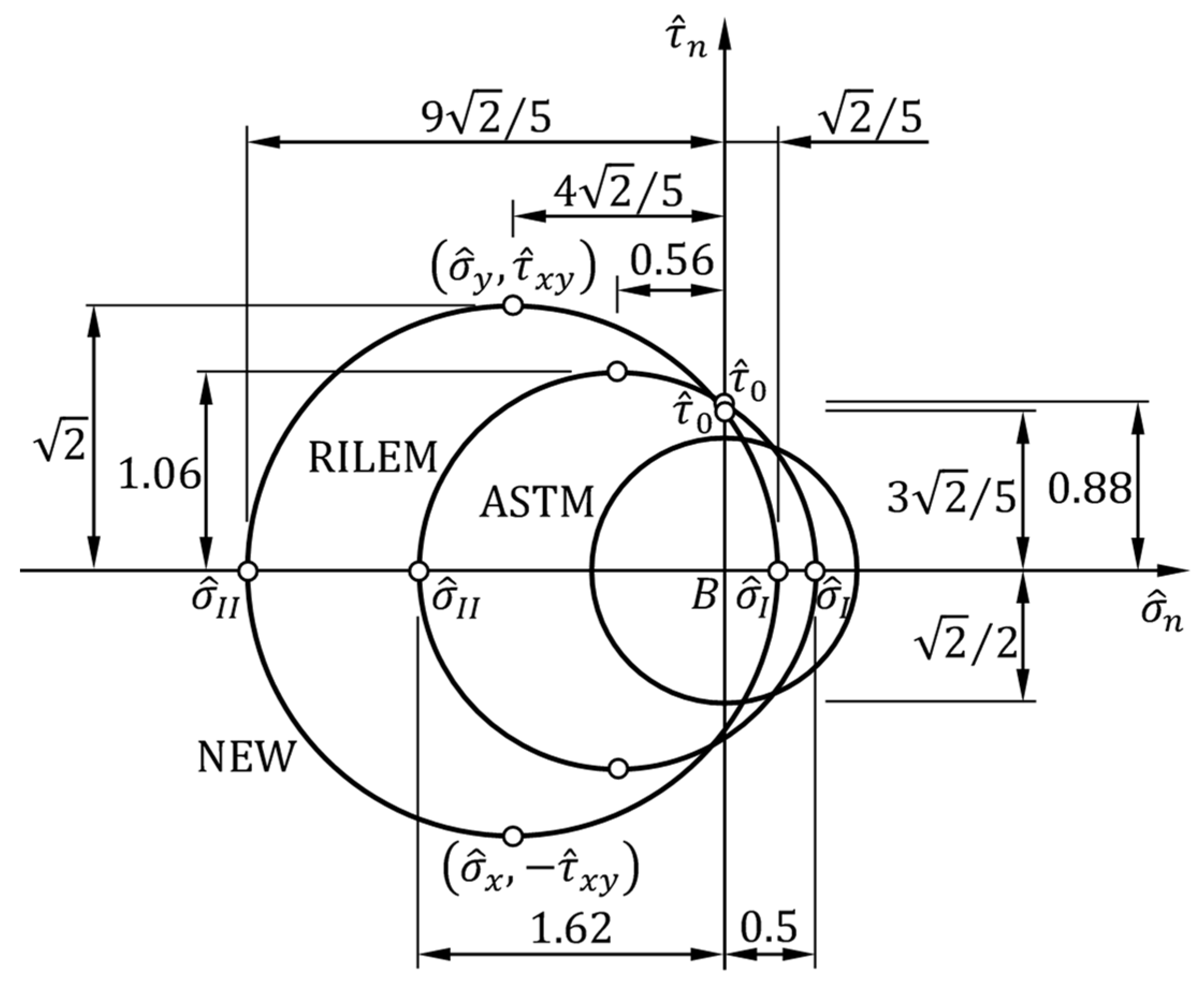
Starting from Equation (92), we can note that the value $k=1$ would cancel the numerator of the equation and, consequently, the value of $E$. Since having $E=0$ is physically unacceptable, we must therefore discard the possibility $k=1$. Ultimately, this is evidence of why the stress field at point $A$ (Figure 1) cannot be a state of pure shear stress, as is the stress state in the ASTM guidelines. In fact, since the state of pure shear stress implies that the two principal stresses have the same (absolute) value, Equation (22) provides precisely the value $k=1$ in the ASTM interpretation of the diagonal compression test. We can therefore conclude that the ASTM assumption of a pure shear stress at point $A$ does not comply with the theory of linear elasticity, because the presence of normal stress components at point $A$ finds justification precisely in the theory of linear elasticity. It is worth noting that even some numerical methods confirmed, in the past, that a square plate made of an elastic isotropic material loaded in diagonal compression does not experience a state of pure shear stress but a complex nonuniform stress state, with normal components different from zero [7,23,24].

Furthermore, since:

$${\epsilon }_v<0,$$

(110)

$$\left|{\epsilon }_v\right|>{\epsilon }_h,$$

(111)

the denominator of Equation (92) is positive for small values of $k$, much lower than 1, while the numerator is positive for $k<1$. This means that $E$ takes positive values in the two intervals:

$$0<k\ll 1,$$

(112)

$$k>1.$$

(113)

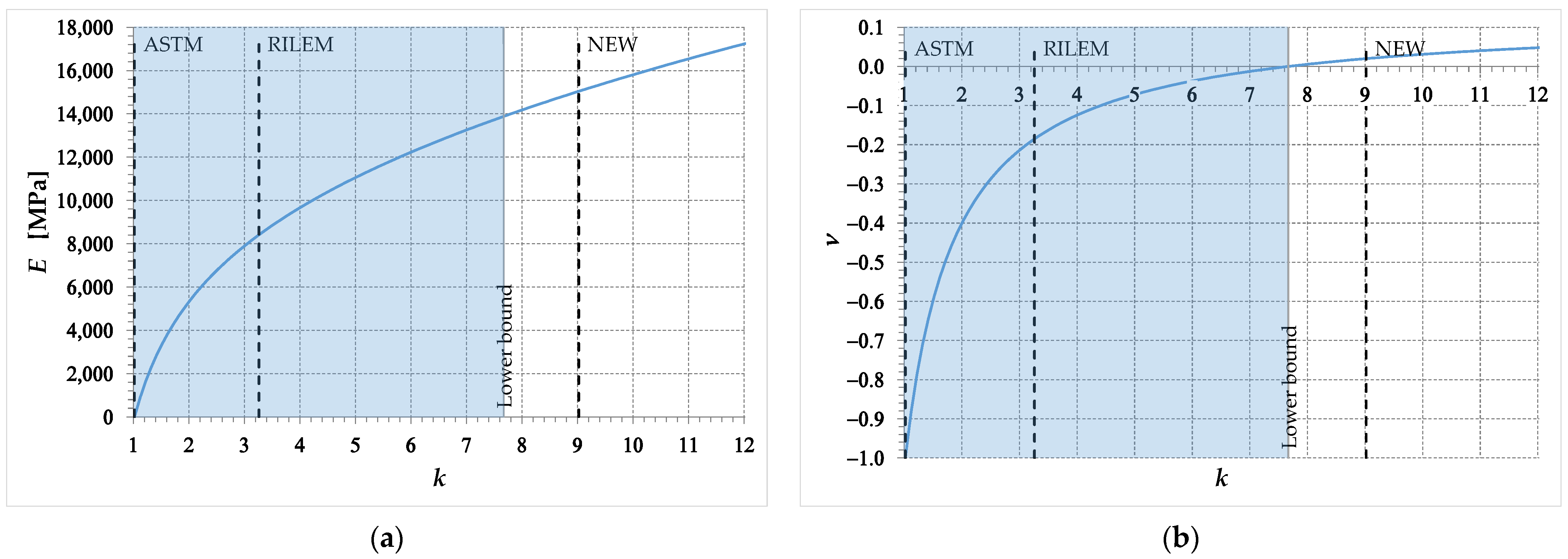
Excluding the possibility $0<k\ll 1$—because it would imply that $f_{dc}\ll f_{dt}$—Equation (113) is the first limitation for $k$.

The second limitation arises from the first inequality in Equation (109), with $\nu$ expressed by Equation (93). For Equations (110), (111) and (113), the denominator in Equation (93) is negative. Therefore, $\nu >0$ if:

$${\epsilon }_t=k{\epsilon }_h+{\epsilon }_v>0,$$

(114)

which provides (in the linear elastic range):

$$k>-\frac{{\epsilon }_v}{{\epsilon }_h}.$$

(115)

Due to the inequality in Equation (111), this second condition is more restrictive than Equation (113). To be precise, the second member in Equation (115) depends on the individual test. However, assuming that the ${-\epsilon }_h/{\epsilon }_v$ ratio does not exceed the value 0.25 (as usually done for the strains along the two diagonals [25,26,27,28]):

$$-\frac{{\epsilon }_h}{{\epsilon }_v}\le 0.25,$$

(116)

it is reasonable to conclude that $k$ is never less than 4. This also raises serious doubts about the validity of the RILEM interpretation of the diagonal compression test, since the value assumed by $k$ in the RILEM guidelines is equal to 3.24 (the inverse of the value in Equation (17)).

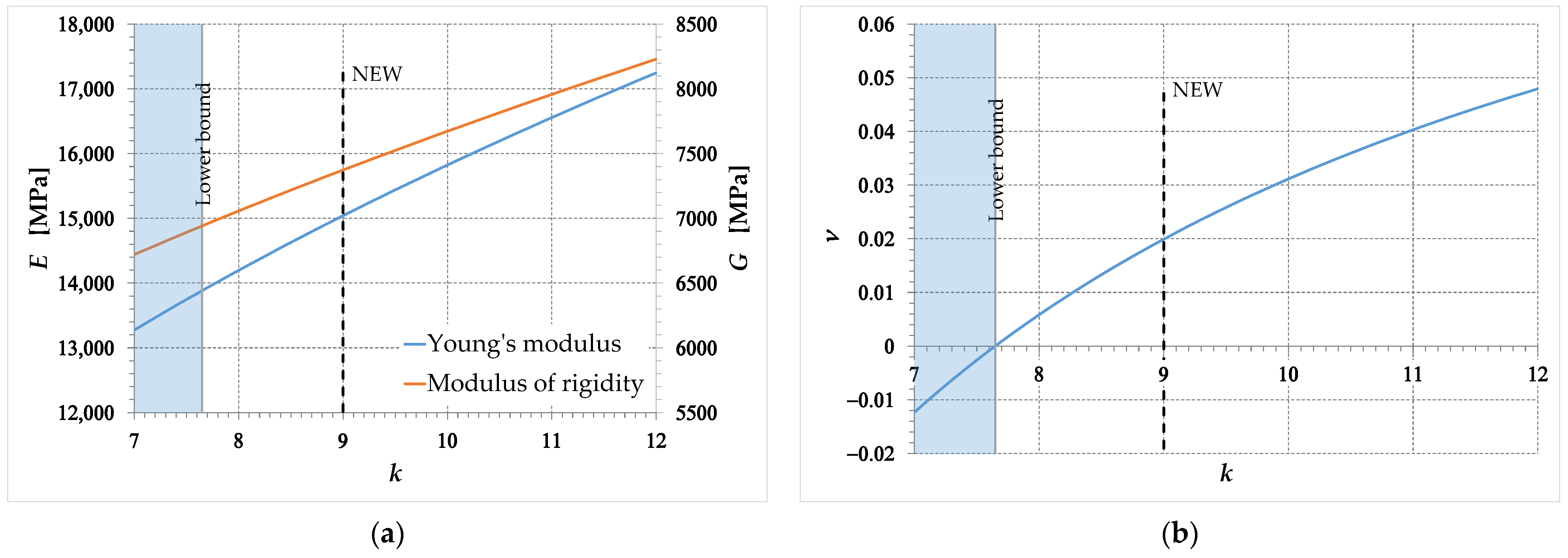
Finally, from the second inequality in Equation (109), it follows that:

$$k>-\frac{\frac{1}{2}{\epsilon }_h+{\epsilon }_v}{\frac{1}{2}{\epsilon }_v+{\epsilon }_h},$$

(117)

which—assuming the validity of Equation (116)—is a less restrictive condition than Equation (115). In conclusion, from the theory of linear elasticity, we can derive the lower limit value (lower bound) for $k$, expressed by Equation (115).

4. How to Identify the Coefficient $\mathit{k}$ and Obtain the Solution

The identification of $k$ requires the comparison of the parametric solution with a certain datum, which can be an elastic coefficient or a stress value. In the impossibility of having this comparison datum, the results provided by the shear-compression test may be useful.

The shear-compression test is another mechanical characterization test for determining the shear strength in masonry [6,15]. It is common opinion that it reproduces the stress state in a masonry element subjected to pure shear stress more faithfully than the diagonal compression test. The results provided by the two tests according to the current legislation are actually very different from each other, as the shear-compression test gives a shear strength value approximately double that of ${\tau }_{xy}^{ASTM}$, the shear strength obtainable through the ASTM interpretation of the diagonal compression test [29,30]:

$${\tau }_{xy}^{ASTM}={\tau }_0^{ASTM}=\frac{\sqrt{2}}{2}\frac{\left|P\right|}{A_n}.$$

(118)

This information provides the comparison datum to identify the coefficient $k$. In fact, in the assumption that both the shear-compression test and the new interpretation of the diagonal compression test provide a realistic representation of the stress state in the specimens, both should give a shear strength value double of that in Equation (118). Therefore, equating Equation (104) to double the value in Equation (118) solves the problem of identifying $k$:

$${\tau }_{xy}^{NEW}=\frac{\sqrt{2}}{4}\left(1+\sqrt{k}\right)\frac{\left|P\right|}{A_n}=\sqrt{2}\frac{\left|P\right|}{A_n}=2{\tau }_{xy}^{ASTM},$$

(119)

which provides the new interpretation of the diagonal compression test in the (modified) Mohr plane:

$$k=9,$$

(120)

$${\widehat{\sigma }}_x^{NEW}={\widehat{\sigma }}_y^{NEW}=-\frac{4}{5}\sqrt{2},$$

(121)

$${\widehat{\tau }}_{xy}^{NEW}=r=\sqrt{2},$$

(122)

$${\widehat{\sigma }}_I^{NEW}=\frac{1}{5}\sqrt{2},$$

(123)

$${\widehat{\sigma }}_{II}^{NEW}=-\frac{9}{5}\sqrt{2},$$

(124)

$${\widehat{\tau }}_0^{NEW}=\frac{3}{5}\sqrt{2},$$

(125)

where the normalized pure shear stress, ${\widehat{\tau }}_0$, acts on planes inclined (to the horizontal plane) at angles $\pm \beta$, with (Equation (34)):

$$\beta \cong 1.249rad\cong 71°{33}^{\prime }54″.$$

(126)

It is worth noting that the value 9 of the coefficient $k=f_{dc}/f_{dt}$ falls within the range of variability of the $f_c/f_t$ ratio for masonry solids:

$$8\le \frac{f_c}{f_t}\le 12.$$

(127)

This is an indirect confirmation of the correctness of the value found for $k$. In fact, as already specified in Section 2, it is reasonable to expect an $f_{dc}/f_{dt}$ ratio not very different from the $f_c/f_t$ ratio, even if the stress state is biaxial rather than uniaxial.

The advantage of having used information given by a different mechanical characterization test rather than identifying $k$ by comparison with the value of an elastic coefficient or stress value is that the solution found here is independent of the single test and the properties of the single specimen. Within the limits of the approximation made by considering the results given by the shear-compression test and the new interpretation of the diagonal compression test as equivalent, this is therefore the exact solution of the stress state at the center of gravity of the wallette.

Figure 9 shows the comparison between the Mohr circles of the ASTM, RILEM, and new interpretations of the diagonal compression test.

As predicted in Reference [10], the center of the new Mohr circle is further from the origin of the axes, $B$ (Figure 9), than is the center of the RILEM circle. This means that the actual hydrostatic stress state at point $A$ is greater than that hypothesized in the RILEM guidelines. On the other hand, the deviatoric stress state at point $A$ is also greater for the new formulation compared to that hypothesized in the RILEM guidelines, since the radius of the new circle is larger than the radius of the RILEM circle. Therefore, the RILEM guidelines underestimate both the hydrostatic and deviatoric stress states at point $A$.

The percentage difference between ${\widehat{\tau }}_0^{RILEM}$ and ${\widehat{\tau }}_0^{NEW}$, the shear stresses at zero normal stress in the RILEM and new interpretations of the diagonal compression test, respectively, is of the order of 3.6%:

$$\frac{{\widehat{\tau }}_0^{RILEM}-{\widehat{\tau }}_0^{NEW}}{{\widehat{\tau }}_0^{RILEM}}\cong 0.0358.$$

(128)

Therefore, the new proposal provides values of ${\widehat{\tau }}_0$ not very different from those obtained by Frocht thanks to photoelasticity. To tell the truth, ${\widehat{\tau }}_0$ has a weak variation for $k>1$ (Figure 10), especially for values of $k$ greater than those assumed in the RILEM guidelines ($k=3.24$).

Therefore, small errors in the evaluation of ${\widehat{\tau }}_0$ would lead to large errors in the evaluation of $k$, particularly in the range $k>3.24$. This means that ${\widehat{\tau }}_0$ is not the most suitable parameter to identify $k$.

The principal stresses in the RILEM and new interpretations of the diagonal compression test, on the contrary, differ considerably. As is evident in Figure 9, in fact, the RILEM principal stresses are the average values between the principal stresses in the ASTM and new interpretations of the diagonal compression test:

$${\widehat{\sigma }}_I^{RILEM}\cong \frac{{\widehat{\sigma }}_I^{ASTM}+{\widehat{\sigma }}_I^{NEW}}{2},$$

(129)

$${\widehat{\sigma }}_{II}^{RILEM}\cong \frac{{\widehat{\sigma }}_{II}^{ASTM}+{\widehat{\sigma }}_{II}^{NEW}}{2}.$$

(130)

The same type of relationship links the normal and tangential stresses on the $x/y$ plane, for the three formulations:

$${\widehat{\sigma }}_x^{RILEM}\cong \frac{{\widehat{\sigma }}_x^{ASTM}+{\widehat{\sigma }}_x^{NEW}}{2},$$

(131)

$${\widehat{\sigma }}_y^{RILEM}\cong \frac{{\widehat{\sigma }}_y^{ASTM}+{\widehat{\sigma }}_y^{NEW}}{2},$$

(132)

$${\widehat{\tau }}_{xy}^{RILEM}\cong \frac{{\widehat{\tau }}_{xy}^{ASTM}+{\widehat{\tau }}_{xy}^{NEW}}{2}.$$

(133)

Regarding the comparison between the principal stresses in the new and ASTM interpretations of the diagonal compression test, the new proposal corrects the first principal stress by a factor of 0.4 and the second principal stress by a factor of 3.6:

$${\widehat{\sigma }}_I^{NEW}=\frac{2}{5}{\widehat{\sigma }}_I^{ASTM},$$

(134)

$${\widehat{\sigma }}_{II}^{NEW}=\frac{18}{5}{\widehat{\sigma }}_{II}^{ASTM},$$

(135)

while the ratio between the two shear stresses at zero normal stress is 1.2, the value given by $c_{{\tau }_0}$ in Equation (57):

$${\tau }_0^{NEW}=\frac{6}{5}{\tau }_0^{ASTM}.$$

(136)

As far as Equation (134) is concerned, it is worth noting that also Reference [31] found a correction factor of 0.4 for the first principal stress, based on a finite element analysis in the linear elastic field.

5. The Elastic Coefficients Obtained for a Real Set of Experimental Data

As shown in Section 3.3, the diagonal compression test allows the identification of Young’s modulus, $E$, and Poisson’s ratio, $\nu$, of masonry walls, although not originally intended for this purpose [25,26,27,28]. As an example of the identification procedure for $E$ and $\nu$, we will use the experimental results of Reference [10], with the strains ${\epsilon }_v$ and ${\epsilon }_h$, calculated as the ratios of the relative displacements along the diagonals to the initial gage lengths along the diagonals:

$${\epsilon }_h=\frac{∆H}{g},$$

(137)

$${\epsilon }_v=\frac{∆V}{g},$$

(138)

where:

• $∆H$ is the extension along the horizontal diagonal;
• $∆V$ is the shortening along the vertical diagonal (the compressed diagonal);
• $g$ is the gage length in the direction of both diagonals (the gage length for the identification of $∆V$ must be equal to the gage length for the identification of $∆H$ [9]).

The specimens of Reference [10] are square masonry wallettes, strengthened with stainless steel straps [32]. However, the strengthening is ineffective in one of the specimens. Therefore, the results of the diagonal compression test performed on that specimen provide the mechanical characteristics of the unreinforced masonry (URM) and are useful for finding the URM elastic moduli.

In the linear elastic range of the URM specimen of Reference [10], the ${-\epsilon }_h/{\epsilon }_v$ ratio took on the value 0.13 (Table 7 of Reference [10]):

$$-\frac{{\epsilon }_h}{{\epsilon }_v}=0.13.$$

(139)

Because of the relationship in Equation (115), this value sets the lower bound for $k$ to be 7.65:

$$k>7.65.$$

(140)

Being greater than the values of $k$ adopted by both the ASTM and RILEM interpretations of the diagonal compression test, the lower bound in Equation (140) confirms that neither the ASTM not the RILEM guidelines conform to linear elasticity theory. In particular, the $k=1$ value of the ASTM guidelines provides unacceptable values for both $E$ (Figure 11a) and $\nu$ (Figure 11b), regardless of the test performed (Equations (92) and (93), respectively):

$$E^{ASTM}=0,$$

(141)

$${\nu }^{ASTM}=-1.$$

(142)

The $k=3.24$ value of the RILEM guidelines provides $E$ values that do not contradict the limiting values for Young’s modulus (Figure 11a), regardless of the test performed:

$$E^{RILEM}>0,$$

(143)

but makes it necessary to evaluate the acceptability of the $\nu$ values (${\nu }^{RIELM}$) on the individual test.

As shown in Figure 11b, the ${\nu }^{RIELM}$ value for the URM specimen of Reference [10] does not comply with the limiting values for the Poisson ratio:

$${\nu }^{RIELM}<0.$$

(144)

The $k=9$ value of the new formulation, on the contrary, generates a Young’s modulus and a Poisson’s ratio that respect the limiting values for both $E$ (Figure 11a) and $\nu$ (Figure 11b).

Figure 12a shows an enlargement of Figure 11a in the $7\le k\le 12$ range (slightly larger than $8\le k\le 12$, the most common range for $k$ in brittle materials), to better appreciate the behavior of the $E$ function in the range of validity of the linear elastic solution. The secondary axis of Figure 12a shows the values of the $G$ function—the third elastic constant—given by Equation (103). Similarly, Figure 12b is the enlargement of Figure 11b in the $7\le k\le 12$ range, useful for appreciating the weak variations of the Poisson ratio in the range of validity of the linear elastic solution.

The values of the three elastic coefficients provided by Equations (92), (93) and (103) for the new formulation are:

$$E=\mathrm{15,041} \mathrm{M}\mathrm{P}\mathrm{a},$$

(145)

$$\nu =0.02,$$

(146)

$$G=7373 \mathrm{M}\mathrm{P}\mathrm{a}.$$

(147)

The value of $\nu$ in Equation (146) may seem completely unreasonable, since it is an order of magnitude lower than 0.25, the value commonly assumed for the Poisson ratio in masonry [25,26,27,28]. This conventional value has no other motivation than that of being the average value between the two limiting values of the Poisson ratio [33]. In reality, although adopted by almost all masonry building codes, 0.25 is a highly questionable value for masonry, since it is the Poisson ratio of cast iron and carpentry steel. Being a brittle material, in fact, masonry should have a Poisson ratio significantly lower than that of a metallic material.

Wanting to find an upper bound for the Poisson ratio in masonry, the $-{\epsilon }_h/{\epsilon }_v$ ratio in Equation (139) could give a first indication. This ratio is actually 48% lower than 0.25. However, there are two observations to make regarding Equation (139). The first observation concerns the ratio itself, which, limited to a uniaxial compression load test performed along the vertical direction, expresses precisely the Poisson ratio. Therefore, since the test performed in Reference [10] is not the uniaxial compression test and the stress state at point $A$ is biaxial, rather than uniaxial, the ratio in Equation (139) does not give the exact value of Poisson’s ratio.

The second observation concerns the scale of acquisitions of the displacements for the identification of the strains. The strains in Equation (139) come from displacements acquired along the entire diagonals, using a horizontal and a vertical potentiometer (produced by Gefran SpA, Brescia, Italy). Well, since micro-cracks propagate in brittle materials even for very low values of the applied load [34], two contributions make up the displacements acquired along the two diagonals: a rheological one (the deformation of the body in the context of continuum mechanics) and a non-rheological one (the opening of micro-cracks). The non-rheological contribution has a particular effect on the acquisition of the displacements along the tensioned diagonal. Therefore, the rheological part in the numerator of Equation (139) could be much lower than the values of ${\epsilon }_h$ identified by the horizontal potentiometer (arranged along the tensioned diagonal). This means that the Poisson ratio identified after excluding the non-rheological contribution could be even much lower than the value provided by Equation (139). Similar observations expressed for another brittle material, namely concrete, suggested acquiring the displacements inside the specimen core that presumably remains intact for the entire duration of the uniaxial compression test, using fiber optic sensors. This allowed us to identify Poisson’s ratio values for concrete, which, for the linear elastic range, are perfectly consistent with the 0.02 value in Equation (146) [34]. Now, the very low values of Poisson’s ratio in the linear elastic range of brittle materials also find an analytical justification.

Equations (122) and (88) then allow us to compare the shear stress–shear strain curves for the three proposals, in the $x/y$ plane (Figure 13). According to Equation (133), the RILEM curve is the average curve between the ASTM curve and the new curve. Due to the assumption in Equation (119), the values of shear stress in the new formulation, ${\tau }_{xy}^{NEW}$, are then double the values assumed in the ASTM curve, ${\tau }_{xy}^{ASTM}$. Therefore, the relationship between the shear stresses in the three formulations (at any given shear strain) is:

$${\tau }_{xy}^{NEW}=2{\tau }_{xy}^{ASTM}=\frac{4}{3}{\tau }_{xy}^{RILEM},$$

(148)

where ${\tau }_{xy}^{RILEM}$ is the shear stress in the RILEM interpretation of the diagonal compression test.

The slope at the origin of the new curve in Figure 13, $G_{xy}^{NEW}$, is equal to the value of $G$ given by Equation (147). Its relationship to the moduli of rigidity in the ASTM and RILEM interpretations of the diagonal compression test, $G_{xy}^{ASTM}$ and $G_{xy}^{RILEM}$, respectively, is the same as that established by Equation (148) between the three shear stresses:

$$G_{xy}^{NEW}=2G_{xy}^{ASTM}=\frac{4}{3}{G}_{xy}^{RILEM}.$$

(149)

As already discussed in Section 3.3, $G_{xy}^{NEW}$ does not depend on the plane ($x/y$ rather than $s/t$) for the calculation of the modulus of rigidity. Consequently, the slope at the origin of the shear stress–shear strain curve is the same in the $x/y$ and $s/t$ planes (Figure 14), with ${\tau }_{st}$ and ${\gamma }_{st}$ given by Equations (125) and (83), respectively (for the value of $\beta$, see Equation (126)).

Finally, Equations (12), (13), (123), (124), (137) and (138) allow us to compare the ${\sigma }_I/{\epsilon }_h$ and ${\sigma }_{II}/{\epsilon }_v$ curves in the RILEM (Figure 15a) and new (Figure 15b) proposals, with the stress–strain curves in compression that occupy the first quadrants and the stress–strain curves in tension that occupy the third quadrants (as usual for brittle materials):

$${{\sigma }^{*}}_I=-{\sigma }_I,$$

(150)

$${{\sigma }^{*}}_{II}=-{\sigma }_{II},$$

(151)

$${{\epsilon }^{*}}_h=-{\epsilon }_h,$$

(152)

$${{\epsilon }^{*}}_v=-{\epsilon }_v.$$

(153)

As specified in Reference [10] and Section 2, the ${{\sigma }^{*}}_I/{{\epsilon }^{*}}_h$ and ${{\sigma }^{*}}_{II}/{{\epsilon }^{*}}_v$ curves in Figure 15b do not represent the stress–strain relationships in uniaxial tension and compression, because the stress state at point $A$ is biaxial (and not uniaxial). Therefore, the slopes at the origin of the ${{\sigma }^{*}}_I/{{\epsilon }^{*}}_h$ and ${{\sigma }^{*}}_{II}/{{\epsilon }^{*}}_v$ curves are not the elastic moduli in uniaxial tension, $E_t$, and compression, $E_c$, respectively (Young’s moduli [35]), with:

$$E_t=E_c=E.$$

(154)

The relationships between ${\sigma }_I$ and ${\epsilon }_h$ and between ${\sigma }_{II}$ and ${\epsilon }_v$, in fact, also depend on the Poisson effect, as expressed by Equations (94) and (95). In this paper, $E_{dt}$ will denote the diagonal tensile elastic modulus (the slope at the origin of the ${{\sigma }^{*}}_I/{{\epsilon }^{*}}_h$ curve), and $E_{dc}$ will denote the diagonal compressive elastic modulus (the slope at the origin of the ${{\sigma }^{*}}_{II}/{{\epsilon }^{*}}_v$ curve), with:

$$E_{dt}\ne E_{dc}.$$

(155)

As noted in Reference [10], the percentage difference between $E_{dt}^{RILEM}$ and $E_{dc}^{RILEM}$, the diagonal tensile and compressive elastic moduli in the RILEM interpretation of the diagonal compression test:

$$\frac{\left|E_{dt}^{RILEM}-E_{dc}^{RILEM}\right|}{E_{dc}^{RILEM}}\cong 136\%,$$

(156)

with:

$$E_{dt}^{RILEM}>E_{dc}^{RILEM},$$

(157)

is too large to depend only on the approximation introduced by neglecting the Poisson effect, which allows us to treat the biaxial stress state as a uniaxial stress state. The percentage difference between $E_{dt}^{NEW}$ and $E_{dc}^{NEW}$, the diagonal tensile and compressive elastic moduli in the new interpretation of the diagonal compression test, is actually an order of magnitude smaller than the value in Equation (156):

$$E_{dt}^{NEW}=\mathrm{12,753} \mathrm{M}\mathrm{P}\mathrm{a},$$

(158)

$$E_{dc}^{NEW}=\mathrm{15,008} \mathrm{M}\mathrm{P}\mathrm{a},$$

(159)

$$\frac{\left|E_{dt}^{NEW}-E_{dc}^{NEW}\right|}{E_{dc}^{NEW}} \cong 15\%.$$

(160)

In particular, the percentage difference between $E_{dc}^{NEW}$ and the value of $E$ in Equation (145) is almost negligible, due to the very low value of the Poisson ratio identified for the specimen (Equation (146)):

$$\frac{\left|E_{dc}^{NEW}-E\right|}{E}\cong 0.2\%.$$

(161)

This allows us to use the ${{\sigma }^{*}}_{II}/{{\epsilon }^{*}}_v$ curve in Figure 15b to obtain the Young modulus as a first approximation. In other words, the stress–strain relationship along the compressed diagonal is representative (with good approximation) of the constitutive law for unreinforced masonry walls in uniaxial compression. Therefore, the new interpretation of the diagonal compression test in the Mohr plane offers a procedure for estimating (with good approximation) the uniaxial stress–strain relationship in compression.

Finally, the diagonal compressive strength and the diagonal tensile strength in the new interpretation of the diagonal compression test (Figure 15b) take on values within the ranges of values for the compressive and tensile strength [36], respectively:

$$f_{dc}\cong 3.52 \mathrm{M}\mathrm{P}\mathrm{a},$$

(162)

$$f_{dt}\cong 0.39 \mathrm{M}\mathrm{P}\mathrm{a},$$

(163)

$$\frac{f_{dt}}{f_{dc}}=\frac{1}{k}=0.\overline{1}.$$

(164)

Due to the observations made regarding Equation (161), the diagonal compressive strength is representative (with good approximation) of the compressive strength for unreinforced masonry walls in uniaxial compression:

$$f_{dc}\cong f_c.$$

(165)

Finally, it is worth noting that $1/k=0.\overline{1}$ is a slightly larger value than the tensile-to-compressive-strength ratio usually identified by uniaxial tensile and compression tests [20]. However, due to the technical difficulties associated with uniaxial tensile tests, it is reasonable to assume that the tensile strength value estimated from uniaxial tensile tests is underestimated. This, together with the difference already noted between the $f_{dt}/f_{dc}$ ratio and $f_t/f_c$ ratio, makes $0.\overline{1}$ a reasonable value for the $f_{dt}/f_{dc}$ ratio.

6. Conclusions

The results of a previous experimental campaign on the shear behavior of masonry wallettes were an opportunity to highlight some inconsistencies in the RILEM interpretation of the diagonal compression test, which represents an improvement of the ASTM interpretation of the diagonal compression test. The present article took inspiration from these inconsistencies and re-examined the state of stress at the center of gravity of the wallette, in the context of the theory of linear elasticity.

The choice made in this paper was to perform the stress analysis in parametric form, as a function of the ratio between the diagonal compressive strength, $f_{dc}$, and the diagonal tensile strength, $f_{dt}$. The extension of the analysis to the strain field then led to the identification of the three elastic coefficients, as functions of the $f_{dc}/f_{dt}$ ratio. This allowed us to demonstrate that both the ASTM and RILEM interpretations of the diagonal compression test do not conform to the theory of linear elasticity. In particular, adopting the ASTM $f_{dc}/f_{dt}$ ratio is equivalent to assuming that Young’s modulus has zero value, which is evidently impossible. Since the ASTM $f_{dc}/f_{dt}$ ratio equals 1—which means that the stress state at the center of gravity, $A$, is a pure shear stress—this is the analytic reason why the stress state at point $A$ of a wallette subjected to a diagonal compression test is not a pure shear stress. This means that, in addition to a deviatoric stress state, a hydrostatic stress state is present at point $A$. Furthermore, both the ASTM and RILEM $f_{dc}/f_{dt}$ ratios would provide negative values for the Poisson ratio, which is an unverified circumstance in natural materials.

The comparison between the stress results of the diagonal compression test and those of the shear-compression test—which is the second useful test for studying the shear behavior of masonry walls—then made it possible to identify the $f_{dc}/f_{dt}$ ratio in the new proposal. This allowed us to obtain an interpretation of the diagonal compression test consistent with the results of the shear-compression test, which is more realistic in describing the shear behavior of masonry walls.

The stress state plot in the Mohr plane showed that the stress field at point $A$ is the sum of a pure shear stress state and a uniaxial compressive stress state, with the planes at zero normal stress inclined at angles equal to $\pm 71°$ with respect to the tensioned diagonal. As in the RILEM guidelines, the center of the new Mohr circle does not lie on the origin of the Mohr plane. However, its distance from the origin is larger than it is in the RILEM guidelines. This means that the RILEM guidelines underestimate the hydrostatic stress state at point $A$. Furthermore, since the radius of the new Mohr circle is larger than the radius of the RILEM Mohr circle, the RILEM guidelines also underestimate the deviatoric stress state at point $A$. As a consequence of the translation of the Mohr circle from the origin, both the ASTM and RILEM guidelines then overestimate the diagonal tensile strength. In particular, the new tensile strength is:

• 40% of the ASTM tensile strength;
• 57% of the RILEM tensile strength.

The new proposal made it possible to rework the experimental results of the previous experimental campaign, in particular those on unreinforced masonry. This led to the identification of a Young’s modulus, $E$, and a Poisson’s ratio, $v$, more consistent with the experimental evidence in uniaxial compression. In particular, the value identified for $v$ agrees in order of magnitude with the experimental results on the Poisson ratio in concrete solids. As it is one order of magnitude lower than the Poisson ratio value usually assumed to identify the Young modulus with both the ASTM and RILEM guidelines, this constitutes a further reason for uncertainty on the elastic modulus obtained with the current standards for the diagonal compression test.

7. Future Developments

As an example of the procedure for identifying elastic moduli, this article has reworked the experimental results of a diagonal compression test on reinforced masonry, with an ineffective reinforcement system. Although the ineffectiveness of the reinforcement made it possible to state that the results obtained are referable to unreinforced masonry (URM), a single experimental test is obviously insufficient to identify the elastic moduli and strength of masonry walls. A proper mechanical characterization, in fact, requires extensive experimental analysis and statistical treatment of the data obtained. Furthermore, we cannot entirely exclude that the reinforcement interventions, even if with ineffective results, have somehow altered the mechanical properties of the masonry. In this sense, the values provided in this article for $E$, $\nu$, $G$, $f_{dc}$, and $f_{dt}$ can only be considered indicative. A large experimental campaign on the shear behavior of the URM is therefore desirable, with results elaborated through the new interpretation of the diagonal compression test.

Finally, it is worth noting that the parametric analysis presented in this article can also be a guide to identifying the shear behavior of other brittle building materials. Among others, rammed earth walls and habitable modules 3D printed with earthen materials deserve a special mention, given the growing interest that these building typologies are gaining recently.