Bridge Damage Detection Using Complexity Pursuit and Extreme Value Theory

Abstract

Bridge structures are susceptible to environmental and operational variations (EOVs). Improperly handling these influences may result in incorrect assessments of the bridge’s health condition. Blind source separation (BSS) techniques show promising potential in suppressing the effects of EOVs. However, major challenges such as high data variability, difficulty in parameter selection, lack of reliable decision thresholds, and practical engineering validation have seriously hindered the application of such techniques in bridge health monitoring. Consequently, this paper proposes a new method for bridge damage detection that combines complexity pursuit (CP) and extreme value theory (EVT). This method first uses the exponentially weighted moving average (EWMA) technique to preprocess the measured modal frequencies. The CP algorithm and information entropy are then used to extract structural damage sources from the preprocessed data automatically. Based on the extracted structural damage sources, the damage index (DI) is defined using k-means clustering and Euclidean distance. Following that, the generalized extreme value (GEV) distribution is used to fit the DI data under the normal condition of the bridge, and the damage detection threshold is given according to the fitted distribution. Benchmark data of the KW51 railway bridge are considered to verify the effectiveness of the proposed method along with several comparative studies. The results show that even under strong EOV influences, the proposed method still maintains good damage detection accuracy and robustness, and its effectiveness is superior to some well-known damage detection methods.

1. Introduction

During the service life of bridges, they inevitably face the combined effects of traffic loads, environmental corrosion, and natural disasters [1]. These influences can lead to the degradation of structural performance and may further induce structural damage or collapse. In recent years, structural health monitoring (SHM) techniques have been increasingly widely used in bridge safety monitoring to avoid catastrophic accidents [2]. SHM includes three main levels: damage detection, damage localization, and damage quantification. Since the necessity of implementing the second and third levels largely depends on the accurate detection of damage, damage detection is crucial to SHM [3]. Data-driven SHM identifies structural damage by observing changes in the dynamic properties of the structure, such as modal frequencies [4]. However, in practical engineering, EOVs such as temperature, humidity, and load can also cause changes in the structural dynamic properties. These changes often mask the true damage of the structure; if the effects of EOVs are not eliminated, the credibility of SHM will be greatly reduced. For this reason, damage detection considering the impact of EOVs has attracted widespread attention from scholars [5,6,7].

In response to this issue, existing methods can be roughly divided into explicit and implicit methods [8]. Explicit methods use statistical or machine learning techniques to establish a correlation model between structural dynamic properties and EOVs. These methods achieve damage detection through the prediction error of dynamic properties in the correlation model or eliminate the influence of EOVs by normalizing dynamic properties [9,10,11,12]. However, there are some difficulties in applying explicit methods to practical engineering projects. The main problem lies in the diversity of EOVs and their complex effects on structural dynamic properties. These factors make it difficult to comprehensively measure various EOVs and accurately model the relationship between EOVs and structural dynamic properties [13,14].

Compared to explicit methods, implicit methods do not require the measurement of EOVs and have better economic and application prospects [15], a review of implicit methods can be found in the literature [16]. In implicit methods, damage detection techniques based on feature extraction are quite common. These methods treat EOV as a latent variable, which can be extracted using feature extraction methods such as principal component analysis (PCA), factor analysis [17], and blind source separation (BSS). Among these, PCA is the most widely applied [18]. The PCA-based damage detection method assumes that the modes of dynamic characteristic changes caused by structural damage and EOVs are different; hence, they can be separated [19]. Yan et al. [20,21] applied linear PCA and local PCA to the damage detection of simulated concrete bridges and Z24 bridges. Considering the nonlinear impact of EOVs on structural dynamic properties, Oh et al. [22] employed kernel PCA, which maps original data to a high-dimensional feature space through kernel transformation, ensuring the linearity of the data. An Auto Associative Neural Network (AANN) has also been used to realize nonlinear PCA [23,24]. Hsu et al. [25] verified the damage detection capability of the AANN method by numerical simulation of the bridge when there is a nonlinear effect of the EOVs on the dynamic properties of the structure. Silva et al. [26] increased the number of layers of the neural network of the AANN method to improve its nonlinear feature extraction capability. Although PCA-based methods have shown relatively good performance in existing studies, linear PCA requires the data to conform to a Gaussian distribution; AANN requires cumbersome network parameter tuning, and kernel PCA is sensitive to kernel parameter selection. These issues limit the promotion of damage detection methods based on PCA in practical engineering applications.

BSS technology provides another solution for structural damage detection under the influence of EOVs. BSS technology originated from the field of acoustics to recover source signals from mixed signals [27]. The idea behind applying BBS technology to damage detection under the influence of EOVs is that changes in structural dynamic properties are jointly caused by random noise, EOVs, and structural damage. Therefore, BSS technology can be used to extract the source signals that represent structural damage. Under this framework, Lin et al. [28] used the AMUSE algorithm to extract structural damage sources from structural modal frequency data. They used pre-stressed concrete beams subjected to temperature effects as numerical cases to validate the feasibility of the proposed method. However, their study is only a preliminary exploration and needs to discuss how to determine the damage detection threshold or the feasibility of the method in actual engineering. Moreover, the AMUSE algorithm has limitations, such as sensitivity to delay parameters and high requirements for source signals non-correlation. Rainieri et al. [29] demonstrated the application of the Second Order Blind Identification (SOBI) algorithm in predicting changes in structural modal frequencies. This method can be used to compensate for the effects of EOVs on structural modal frequencies without the need to measure EOVs. However, the authors did not use the proposed method in practical structural damage detection.

Existing research shows that BBS technology has promising potential for damage detection under the influence of EOVs. However, to the best of the authors’ knowledge, research in this area is still very lacking. To apply BBS technology more effectively to damage detection under the influence of EOVs, we face two main challenges. Firstly, the BBS algorithm must have good universality, meaning it should apply to situations where source signals exhibit nonlinear mixing, and it should also reduce reliance on expert experience, making it more user-friendly. Secondly, to improve the accuracy of damage detection, it is necessary to come up with appropriate methods for determining damage detection thresholds. To address these issues, this paper introduces the CP algorithm for extracting structural damage sources and establishes the damage thresholds using the extreme value theory. CP as a new BSS technology has been introduced in studies [30,31,32,33] to decompose the vibrational response of structures into individual modal contributions. Compared to other renowned BSS methods, such as ICA and SOBI, the CP algorithm has been proven to have numerous advantages, including computational efficiency, user-friendliness, and better separation capabilities for tightly spaced and highly correlated source signals. In the field of structural damage detection, extreme value theory is commonly used to avoid treating damage index data as normally distributed and then applying the central limit theorem to determine the damage detection threshold. There has been much research on damage detection based on extreme value theory [34,35,36,37,38]. Compared to existing research, the main advantage of the method presented in this paper lies in the introduction of the CP algorithm to suppress the strong EOV interference in damage detection. At the same time, the proposed method automatically determines extreme value samples based on KL divergence, avoiding the uncertainty and cumbersome operations brought about by empirical or graphical methods.

The rest of the paper is organized as follows. Firstly, the theoretical basis is presented in Section 2. The implementation procedure of the proposed method is given in Section 3. The performance of the proposed method is verified using KW51 railway bridge vibration data in Section 4. The conclusion is given in Section 5.

2. Theoretical Basis

The bridge damage detection method proposed in this paper mainly consists of the following four parts: (1) Data preprocessing; (2) Using the CP algorithm to extract sources of structural damage; (3) Establishment of damage indicators based on the clustering idea; (4) Establishment of damage detection thresholds based on extreme value theory.

2.1. Data Preprocessing

In finance, statistics, and signal processing, EWMA is often used to smooth data, reduce noise, and capture data trends and changes. This paper uses EWMA as a data preprocessing method, aiming to improve the noise robustness of the proposed method. For time series data $\left\{y_1,y_2,\dots ,y_n\right\}$, its EWMA value is calculated as

$${\overline{y}}_i=\alpha y_i+\left(1-\alpha \right){\overline{y}}_{i-1}$$

(1)

where ${\overline{y}}_i$ represents the EWMA value of the ith data point and $\alpha$ is the weighting factor.

2.2. Using the CP Algorithm to Extract Sources of Structural Damage

Considering a set of measurement data $x(t)={[x_1(t),\dots ,x_m(t)]}^{\mathrm{T}}$ with $m$ dimensions, it is assumed to be formed by $n$ source signals $s(t)={[s_1(t),\dots ,s_n(t)]}^{\mathrm{T}}$ mixed through matrix A.

$$x(t)=As(t)={\displaystyle \sum _{i=1}^n{a}_i{s}_i(t)}$$

(2)

where $a_i$ is the $i$ column in the mixing matrix A.

The goal of the CP algorithm is to find the demixing vector $W_i$, which separates the source signal from the mixed signal

$$y_i(t)=W_{i}x(t)$$

(3)

The CP algorithm assumes that the source signals have less temporal predictability than the mixed signals. The time predictability is evaluated by the function $F(\cdot )$

$$F(y_i)=\log \frac{V(y_i)}{U(y_i)}=\log \frac{{\displaystyle {\sum }_{t=1}^N{({\overline{y}}_i(t)-y_i(t))}^2}}{{\displaystyle {\sum }_{t=1}^N{({\widehat{y}}_i(t)-y_i(t))}^2}}$$

(4)

Among them,

$$\begin{array}{ll}{\overline{y}}_i(t)={\lambda }_L{\overline{y}}_i(t-1)+(1-{\lambda }_L)y_i(t-1)& 0\le {\lambda }_L\le 1\\ {\hat{y}}_i(t)={\lambda }_S{\hat{y}}_i(t-1)+(1-{\lambda }_S)y_i(t-1)& 0\le {\lambda }_S\le 1\end{array}$$

(5)

where $V(\cdot )$ represents the overall change of $y_i(t)$, which characterizes the long-term prediction error of $y_i(t)$. $U(\cdot )$ represents the local smoothness of $y_i(t)$, which characterizes the short-term prediction error of $y_i(t)$. ${\overline{y}}_i(t)$ and ${\widehat{y}}_i(t)$ are the long-term and short-term prediction values of $y_i(t)$, respectively. $\lambda =2^{-1/h}$, $h_s=1$, $h_L$ is an arbitrary value, which only needs to be satisfied $h_L\gg h_S$.

Bringing Equation (3) into Equation (4) gives

$$F(y_i)=F(W_i,x)=\log \frac{V(W_i,x)}{U(W_i,x)}=\log \frac{W_i\overline{R}{W}_i^T}{W_i\widehat{R}{W}_i^T}$$

(6)

where $\overline{R}$ and $\widehat{R}$ are the long-term covariance matrix and the short-term covariance matrix of the measured data, defined as

$$\begin{array}{l}{\overline{R}}_{ij}={\displaystyle \sum _i^N\left(x_i(t)-{\overline{x}}_i(t)\right)}\left(x_j(t)-{\overline{x}}_j(t)\right)\\ {\widehat{R}}_{ij}={\displaystyle \sum _i^N\left(x_i(t)-{\widehat{x}}_i(t)\right)\left(x_j(t)-{\widehat{x}}_j(t)\right)}\end{array}$$

(7)

The gradient ascent technique is applied to solve the demixing vector $W_i$. According to Equation (6), the derivative of the time predictability function $F(\cdot )$ for $W_i$ is

$${\nabla }_W{}_i\mathrm{F}=\frac{2W_i}{V_i}\overline{R}-\frac{2W_i}{U_i}\widehat{R}$$

(8)

To find the maximum value of the time predictability function $F(\cdot )$, make both sides of Equation (8) equal to zero, which yields

$$W_i\overline{R}=\frac{V_i}{U_i}{W}_i\widehat{R}$$

(9)

Equation (9) formulates the BSS problem based on the time predictability function as solving a generalized eigenproblem. The eigenvectors of the matrix ${\widehat{R}}^{-1}\overline{R}$ are the unmixing vectors $W_i$. Finally, the source signal can be obtained according to Equation (3).

In addition, it should be noted that, like other blind source separation methods, the source signals obtained by the CP algorithm have amplitude uncertainty issues. However, this does not affect its application in structural damage identification because the valuable information relevant to structural damage is mainly contained in the waveform of the source signals. This paper automates the selection of structural damage sources from separated source signals based on information entropy [39]. The information entropy is calculated as

$$\mathrm{H}(y_i)=-\sum _{j=1}^{m}p\left(y_{ij}\right)\log \left(p\left(y_{ij}\right)\right)$$

(10)

where $p(\cdot )$ denotes the probability and $y_{ij}$ denotes the jth element of the ith source signal.

Compared to random noise and EOV, the inherent properties of the structure have lower uncertainty. Therefore, this paper selects the source signal corresponding to the smallest information entropy as the source of structural damage.

2.3. Establishment of DI Based on Clustering Idea

After obtaining the structural damage source, the DI is established based on the clustering idea. The process first uses a clustering algorithm to calculate the clustering center of structural damage sources under the normal condition of the bridge, and then the minimum distance from structural damage sources to the clustering center is taken as the DI. In this paper, a k-means clustering algorithm is used, assuming that $X=[{\mathbf{x}}_1,\dots ,{\mathbf{x}}_n]\in R^{q\times n}$ is the structural damage source, and the k-means clustering objective function is expressed as

$$J\left(c_1,\dots ,c_k\right)=\min \sum d\left({\mathbf{x}}_i,{\mathbf{c}}_j\right)$$

(11)

where $c_1,\dots ,c_k$ is the clustering center and $d$ denotes the value of the distance.

The k-means clustering algorithm updates the cluster centers by minimizing the value of the objective function until the cluster centers no longer change. When Euclidean distance is used as the distance metric, the DI is defined as

$$\mathrm{DI}=\min \left(\Vert {\mathbf{x}}_i-{\mathbf{c}}_1\Vert ,\Vert {\mathbf{x}}_i-{\mathbf{c}}_2\Vert ,\dots ,\Vert {\mathbf{x}}_i-{\mathbf{c}}_3\Vert \right)$$

(12)

The number of clusters needs to be specified for k-means clustering. For bridge damage detection under the influence of EOVs, the appropriate number of clusters should result in small variability in DI values corresponding to the normal condition of the bridge. In this paper, the median absolute deviation (MAD) is used to measure the variability of DI. The MAD is calculated as

$$\mathrm{MAD}(\mathrm{DI})=\mathrm{median}\left(\left|y_i-\mathrm{median}(\mathrm{DI})\right|\right)$$

(13)

where $y_i$ is the element in the DI dataset, and the median is the median operation.

The MAD value of DI data decreases as the number of clusters increases, but too many clusters can cause the model to overfit the training samples. In this paper, the corresponding number of clusters when the MAD value of DI data tends to stabilize is determined as a reasonable number of clusters.

2.4. Establishing Damage Detection Thresholds Based on EVT

This paper applies EVT to establish robust damage detection thresholds. EVT is a method of modeling the tails of a probability distribution of a random variable using extreme values. EVT includes the BMM model and the POT model. The BMM model is used in this paper.

Suppose $X_1,X_2,\dots ,X_n$ is an independent identically distributed random variable with an unknown global distribution. According to the Fisher–Tippett extreme value type theorem [40], regardless of the form of the global distribution, if the asymptotic distribution of the maximum value of the random variable exists and is nondegenerate, one of the Gumbel, Frechet, and Weibull distributions can be used to describe the extreme value sample. These three distributions can be uniformly represented by the GEV distribution

$$g(x)=\{\begin{array}{ll}\exp \left[-{\left(1+\xi \frac{x-\mu }{\sigma }\right)}^{-1/\xi }\right]& \xi \ne 0\\ \exp \left[-\exp \left(-\frac{x-\mu }{\sigma }\right)\right]& \xi =0\end{array}$$

(14)

where $\xi$ is the shape parameter, $\sigma$ is the scale parameter, and $\mu$ is the position parameter. When $\xi =0$, the GEV formula corresponds to the Gumbe distribution; when $\xi >0$, the GEV formula corresponds to the Frechet distribution; and when $\xi <0$, the GEV formula corresponds to the Weibull distribution;

The log-likelihood function of Equation (14) can be expressed as

$$\begin{array}{l}L(\xi ,\sigma ,\mu )=-\left(1+\frac{1}{\xi }\right){\displaystyle \sum _{i=1}^p\ln \left[1+\frac{x_i-\mu }{\sigma }\right]}-p\ln \sigma -{\displaystyle \sum _{i=1}^p{\left[1+\frac{x_i-\mu }{\sigma }\right]}^{-1/\xi }}\hspace{0.17em}\xi \ne 0\\ L(\sigma ,\mu )=-{\displaystyle \sum _{i=1}^p\log \left[1+\frac{x_i-\mu }{\sigma }\right]}-p\log \sigma -{\displaystyle \sum _{i=1}^p\left[1+\frac{x_i-\mu }{\sigma }\right]}\hspace{0.17em}\hspace{0.17em}\hspace{0.17em}\hspace{0.17em}\xi =0\end{array}$$

(15)

where $p$ is the number of extreme samples, $x_i$ is the extreme sample.

The BMM model divides the random variables into several regions without intersection based on a specific criterion and then selects the extreme values in each region to form extreme value samples. Equation (15) is derived for the parameters of the GEV distribution, and an estimate of the unknown parameters can be obtained by making the derivative zero. Finally, the damage threshold is obtained based on the inverse function of the GEV distribution

$$th{r}_{GEV}=\{\begin{array}{ll}\mu -\frac{\sigma }{\xi }\left(1-{(-\log (1-\alpha ))}^{-\xi }\right)& \xi \ne 0\\ \mu -\sigma \log (-\log (1-\alpha ))& \xi =0\end{array}$$

(16)

In this paper, we avoid using empirical methods to determine the extreme samples for the BMM model based on the Kullback–Leibler (KL) divergence [41]. The KL divergence can describe the degree of difference between two probability distributions, which is defined as

$$D_{\mathrm{KL}}(p\parallel q)=\sum _{x\in \mathsf{\Omega }}p(x)\log \frac{p(x)}{q(x)}$$

(17)

where $p(x)$ and $q(x)$ are two probability distributions in the probability space, and the smaller the value of $D_{\mathrm{KL}}(p\parallel q)$, the closer the two probability distributions are.

In this paper, the specific way to determine the extreme samples based on KL divergence is as follows:

(1) The DI data are arranged in descending order, and different numbers of DI data are taken out in turn as the extreme value samples, and the extreme value samples are fitted with the GEV distribution.

(2) The quantile function of the extreme samples is taken as $p(x)$ and the inverse function of the fitted GEV distribution is taken as $q(x)$. $p(x)$ and $q(x)$ are utilized to solve for the sample values at different quantiles.

(3) Bring the sample values into Equation (16). Select the extreme sample corresponding to the minimum KL divergence value.

3. The Implementation Process of the Proposed Method

The implementation process of the method proposed in this paper consists of two parts: an offline learning phase aimed at constructing a damage detection model and determining the damage detection thresholds, and an online monitoring phase aimed at identifying bridge damage in unknown conditions.

3.1. Offline Learning Stage

1. The measured modal frequencies corresponding to the normal condition of the bridge are used as the training set data, and EWMA technology is used to preprocess the training set data.

2. The CP algorithm and information entropy are used to extract the source of structural damage from the preprocessed data, while the separation matrix W is recorded.

3. The k-means clustering is used to calculate the clustering centers of the structural damage sources, and the DI is calculated according to Equation (12). The number of clusters for the k-means clustering is selected according to the MAD value of the DI.

4. The KL divergence is used to determine the extreme samples of the BMM model, and the GEV distribution is used to fit the extreme samples. The damage detection threshold under a specified confidence level is determined according to Equation (16).

3.2. Online Damage Stage

1. The measured modal frequencies corresponding to the unknown condition of the bridge are used as the test set data, and EWMA technology is used to preprocess the test set data.

2. The information entropy and the separation matrix W obtained from the offline learning phase are used to extract the structural damage sources from the test set data according to Equation (3).

3. The DI during the online detection phase is calculated according to Equation (12).

4. Compare whether the DI value in the detection phase exceeds the damage detection threshold. If it exceeds, it indicates that the bridge has been damaged.

4. Application on KW51 Railway Bridge

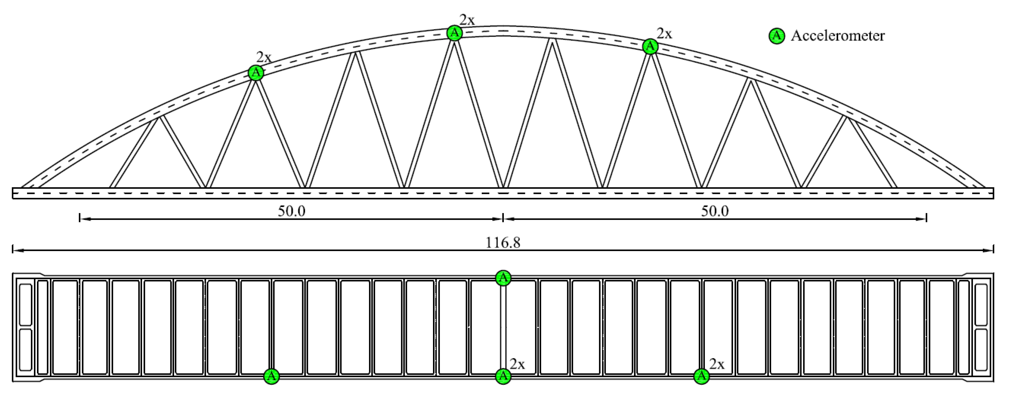
4.1. Bridge Description

This paper uses vibration data from the KW51 railway bridge in Belgium to verify the effectiveness of the proposed method. The KW51 railway bridge is 115 m long and 12.4 m wide and is located on the L36N railroad line between Leuven and Brussels. The SHM system was installed on the bridge on 2 October 2018. Twelve uniaxial accelerometers were mounted on the deck and arche of the bridge to monitor the vibrations of the bridge, as shown in Figure 1.

Due to construction errors, the bridge was retrofitted from 15 May to 27 September 2019. Maes and Lombaert used acceleration data from the SHM system and the Operational Modal Analysis (OMA) method to determine the 1st to 14th modal frequencies of the bridge [42]. The bridge was considered to be in normal condition (NC) before retrofitting and in a damaged condition (DC) after retrofitting, respectively [43,44]. In this paper, as in the literature [43,44], the 6th, 10th, 12th, and 13th-order modal frequencies are chosen for damage detection. These modes correspond to the 2nd to 5th vertical vibration modes of the bridge. After the bridge retrofit, the modal frequency increased. In this paper, the modal frequency after the bridge retrofit is multiplied by 0.99 to amplify the effect of EOV.

Due to variations in the recognizability of structural modes under random excitation, there are missing values in the modal frequency samples. After deleting samples with missing values, 3130 samples are obtained, as shown in Figure 2a. The literature [42] gives the air temperature data around the KW51 railway bridge, which are temporally consistent with the modal frequency data. Figure 2b shows the air temperature data corresponding to the modal frequency data in Figure 2a.

As can be observed from Figure 2, temperature affects different modal frequencies to varying extents. Between samples 1350 and 1600, the low-temperature environment caused a dramatic change in modal frequency, with a magnitude more significant than that caused by the simulated damage [43]. This implies that environmental temperature can mask structural damage, possibly leading to an incorrect assessment of the bridge’s health condition.

For damage detection of the KW51 bridge, modal frequency measurements belonging to the normal condition are used as the training set, the first 90% of the data in the training set are used for training (samples 1–2419), and the remaining 10% of the data are used for validation (samples 2420–2688), and modal frequency measurements belonging to the damaged condition are used as the test set for damage detection (samples 2689–3130).

4.2. Damage Detection

This paper uses the EWMA technique for data preprocessing to enhance the noise robustness of the proposed method. The weighting coefficient can be adjusted based on the noise intensity. When the weighting coefficient is larger, the data processed using the EWMA technique better reflects the timeliness of the original data, but its noise reduction effect is diminished. According to the above principle, after many explorations, in this paper when no artificial noise is added, the weighting factor is set to 0.2, and in other cases, the weighting factor is set to 0.02. Then, the CP algorithm and information entropy are used to extract the structural damage source from the preprocessed data. The parameters $h_s$, $h_L$ of the CP algorithm are set to 1 and 90,000,000, respectively (the parameter settings are kept unchanged for all examples in this study). As shown in Figure 3, the CP algorithm successfully separates four source signals.

As shown in Figure 3, the first separated component corresponds to the change in dynamic properties caused by structural damage, the second and third components correspond mainly to the effects of random noise, while the fourth component corresponds to the change in dynamic properties due to EOV. Information entropy is utilized as an index to select the source signal representing structural damage from the separated results. The information entropy values for the four components are 0, 2.71, 0.18, and 3.65, respectively. Since structural intrinsic properties typically have lower uncertainty than noise and EOVs, the component with the minimum information entropy is selected as the source of structural damage. Based on this criterion, the first separated component is selected. As illustrated in Figure 3a, this component remains relatively stable during the training and validation stages but shows significant differences in the testing stage compared to the previous two. This observation indicates that the extracted structural damage source can accurately reflect changes in structural conditions and is less affected by EOVs.

After obtaining the structural damage source, the DI is established based on k-means clustering. The reasonable number of clusters is determined by analyzing the MAD value of the DI under the normal condition of the bridge. Figure 4a shows the MAD values of DI under different cluster numbers, and it can be seen that when the number of clusters is 100, the MAD value begins to stabilize. Therefore, the number of clusters is determined to be 100.

Based on the KL divergence, this paper selects extreme samples from the DI under the normal condition of the bridge (see Section 2.4 for specific steps). Figure 4b shows the KL divergence values for different numbers of extreme samples. Considering that the optimal number of extreme samples corresponds to the smallest KL divergence value, the number of extreme samples is determined to be 18.

The selected extreme value samples are fitted with the GEV distribution, and the location parameter ($\mu$), scale parameter ($\sigma$), and shape parameter ($\xi$) of the distribution are obtained as 0.002, 0.200, and −0.141, respectively. Under a significance level of 0.05, the damage detection threshold is calculated by Equation (16), and its value equals 0.0023. Figure 5 displays the damage detection results of the proposed method applied to the KW51 railway bridge.

Figure 5 shows that the DI values of the bridge in normal condition are very stable, which indicates that the proposed method can effectively prevent DI from being affected by EOV. Simultaneously, a significant difference exists between the DI values of the bridge under normal and damaged conditions, indicating that the proposed method can effectively distinguish changes in structural health conditions. Moreover, during the training phase (samples 1–2419) and validation phase (samples 2420–2688), only two DI values exceeded the damage detection threshold. In contrast, during the damage detection phase (samples 2689–3130), all the DI values surpass the threshold, highlighting the accuracy of the threshold determination method proposed.

4.3. Comparisons

To investigate the impact of different amounts of training data on the proposed method, the sample training ratio is reduced to 65%, 45%, 25%, and 10%, respectively. Figure 6 shows the damage detection results of the proposed method under these sample training ratios.

Figure 5 and Figure 6 show that Type II errors (false negatives) do not occur under the examined sample training rates. As the sample training rate decreases, the Type I (false positive) error rate increases. Specifically, when the sample training rate is 90%, the Type I error rate is 0.07%. Under the other four sample training rates, the Type I error rates are 0.33%, 0.74%, 4.35%, and 28.01%, respectively. From the above results, it can be seen that when the sample training rate reaches 45%, its impact on the performance of the proposed method is not significant. It is worth noting that when the training sampling rate drops to 45%, due to the lack of changes caused by environmental temperature in the training data, the reliability of the damage detection method usually drops sharply [43,45]. However, the method proposed in this paper does not have this problem, indirectly proving the superiority of the proposed method. When the sample training rate drops to 25%, the Type I error rate increases significantly. These results indicate that although the proposed method performs well at lower sample training rates, to ensure high accuracy of damage detection results in actual use, the training data should include the effects of EOVs as much as possible.

To evaluate the performance of the proposed method on small sample datasets, data are extracted from the original training and test sets at intervals of 9 samples to form new training and test sets. The sample training rate of the new training set remained at 90%. The damage detection results obtained by the proposed method are shown in Figure 7.

As can be seen from Figure 7, under the small sample dataset, there are still no Type II errors in the damage detection results, and only five samples have Type I errors. This indicates that the proposed method has good applicability on small sample datasets.

The above results are based on the original measurement data. To assess the robustness of the proposed method to noise, we add 1% (with respect to the signal, equal to a signal-to-noise ratio (SNR) of 40dB) rms (root-mean-square) Gaussian white noise to the original measurement data [46]. Under the influence of noise, the damage detection results of the method proposed in this paper are shown in Figure 8.

As shown in Figure 8, the Type II error rate in the damage detection results increased under the influence of noise. Although the Type II error rate reached 4.98%, it is still within an acceptable range. It should be noted that this study amplifies the effect of EOVs by reducing the magnitude of the modal frequency change after bridge damage, which also increases the difficulty of damage detection under noisy conditions. Overall, the proposed method demonstrates good noise robustness.

The above results are based on four mixed signals, i.e., the 6th, 10th, 12th, and 13th order modal frequencies are used for damage detection. To analyze the effect of the number of mixed signals on the performance of the proposed method, the number of mixed signals is reduced to three and two, respectively. The comparative study employs the same data as Figure 5 (using all available measured samples without adding noise, with a sample training ratio of 90%). To ensure the objectivity and fairness of the comparison, all parameters except the combination of modal frequencies remain consistent. For the sake of simplicity, the damage detection results are presented in tabular form (see

Table 1. Number and percentage of Type I, Type II, and total errors with different modal frequency combinations.

Modal Frequency Combinations	Type I	Type II	Total
6, 10, 12, 13	2 (0.07%)	0 (0.00%)	2 (0.06%)
6, 10, 12	9 (0.33%)	3 (0.68%)	12 (0.38%)
6, 10, 13	8 (0.30%)	1 (0.23%)	9 (0.29%)
6, 12, 13	5 (0.19%)	0 (0.00%)	5 (0.16%)
10, 12, 13	3 (0.11%)	1 (0.23%)	4 (0.13%)
6, 10	7 (0.26%)	50 (11.31%)	57 (1.82%)
6, 12	8 (0.30%)	2 (0.45%)	10 (0.32%)
6, 13	7 (0.26%)	1 (0.23%)	8 (0.26%)
10, 12	5 (0.19%)	250 (56.56%)	255 (8.15%)
10, 13	4 (0.15%)	3 (0.68%)	7 (0.22%)
12, 13	5 (0.19%)	141 (31.90%)	146 (4.66%)

).

From Table 1, it can be seen that as the number of mixed signals decreases, the performance of the proposed method shows a downward trend. When using three mixed signals, the maximum Type I and Type II error rates are 0.33% and 0.68%, respectively, indicating that the decline in performance of the proposed method is not significant. However, when only using two mixed signals, different modal frequency combinations significantly affect the damage detection results. For example, when using the 10th and 12th order modal frequencies as input, the Type II error rate reached 56.56%. The above results can be explained in terms of blind source separation: The CP algorithm requires that the number of mixed signals is greater than or equal to the number of source signals. If the changes in modal frequencies are caused by a mix of noise, EOVs, and structural damage, when using the CP algorithm to extract the structural damage source, the number of mixed signals should be no less than three to achieve stable and accurate results.

Finally, the proposed method is compared with the well-known PCA and AANN. It should be noted that when the above two methods are applied to damage detection, the damage detection threshold is determined based on the central limit theorem, and the significance level remains at 0.05 [47]. The comparative study employs the same data as Figure 5. The first two principal components are selected for the PCA method, with a cumulative variance contribution rate of 86.6%. The parameters for the AANN method are set as the number of neurons in the input layer, extraction layer, bottleneck layer, reconstruction layer, and output layer, being 4, 5, 2, 5, and 4, respectively. Transfer functions for the extraction and reconstruction layers are hyperbolic tangent, while the other layers are linear. After 2000 trainings, the extracted nonlinear principal components account for 86.4% of the cumulative variance contribution. Figure 9 shows the damage detection results of the above methods.

As shown in Figure 9, regardless of the damage detection threshold setting, none of the above methods can avoid Type II errors with a very low Type I error rate. Comparing Figure 5 and Figure 9, it can be seen that the proposed method has better performance in suppressing the effect of EOV on DI and in identifying the change of structural condition (i.e., enlarging the difference of DI values in different structural conditions).

Table 2. Number and percentage of Type I, Type II, and total errors with different methods.

Method	Type I	Type II	Total
PCA	63 (2.34%)	2 (0.47%)	65 (2.04%)
AANN	67 (2.49%)	7 (1.58%)	74 (2.36%)
The method proposed in this paper	2 (0.07%)	0 (0.00%)	2 (0.06%)

presents the error rates of damage detection for different methods. From Table 2, it can be seen that, whether it is Type I error rate or Type II error rate, the method proposed in this paper demonstrates higher accuracy compared to PCA and AANN.

5. Conclusions

The dynamic properties of bridges are susceptible to the effects of EOVs. Ignoring or improperly handling these effects can greatly reduce the credibility of bridge health monitoring. Therefore, this paper proposes a new damage detection method that integrates the CP algorithm and extreme value theory. The main contribution of this study is the introduction of the high-performance CP algorithm to effectively suppress the impact of strong EOV on damage detection, and the proposal of a new probabilistic method for estimating the damage detection threshold. The effectiveness of the proposed method has been validated by the full-scale KW51 railway bridge case, and the main conclusions are as follows:

(1) The proposed method can effectively reduce the negative impact of EOV on damage detection and exhibit good damage detection accuracy and robustness to noise.

(2) The proposed method still performs well in situations with a low sample training rate and small sample datasets. However, to ensure accurate damage detection results, the training data should include the effects of EOV as much as possible.

(3) The number of mixed signals (modal frequencies) used for damage detection will influence the proposed method’s performance. Considering the assumption of blind source separation techniques for damage detection, it is recommended to use at least three modal frequencies in the analysis to obtain stable and high-precision damage detection results.

(4) Compared with the well-known PCA and AANN, the proposed method shows advantages regarding damage detection precision and the discrimination of structural condition changes.

(5) The proposed method does not require the measurement of EOVs and has good application prospects in practical engineering.

References

1. Kaewunruen, S.; Sresakoolchai, J.; Ma, W.; Phil-Ebosie, O. Digital twin aided vulnerability assessment and risk-based maintenance planning of bridge infrastructures exposed to extreme conditions. Sustainability 2021, 13, 2051. [Google Scholar]
2. Alokita, S.; Rahul, V.; Jayakrishna, K.; Kar, V.; Rajesh, M.; Thirumalini, S.; Manikandan, M. Recent advances and trends in structural health monitoring. In Structural Health Monitoring of Biocomposites, Fibre-Reinforced Composites and Hybrid Composites; Woodhead Publishing: London, UK, 2019; pp. 53–73. [Google Scholar]
3. Daneshvar, M.H.; Sarmadi, H. Unsupervised learning-based damage assessment of full-scale civil structures under long-term and short-term monitoring. Eng. Struct. 2022, 256, 18. [Google Scholar] [CrossRef]
4. Zheng, H.; Duan, Z.D. Structural damage alert with consideration of the nonlinear environmental effects. J. Vib. Eng. 2022, 34, 1101–1111. [Google Scholar]
5. Sohn, H. Effects of environmental and operational variability on structural health monitoring. Philos. Trans. R. Soc. A-Math. Phys. Eng. Sci. 2007, 365, 539–560. [Google Scholar] [CrossRef]
6. Fallahian, M.; Khoshnoudian, F.; Meruane, V. Ensemble classification method for structural damage assessment under varying temperature. Struct. Health Monit. 2018, 17, 747–762. [Google Scholar] [CrossRef]
7. Maes, K.; Van Meerbeeck, L.; Reynders, E.P.B.; Lombaert, G. Validation of vibration-based structural health monitoring on retrofitted railway bridge KW51. Mech. Syst. Signal Process. 2022, 165, 24. [Google Scholar] [CrossRef]
8. Mousavi, M.; Gandomi, A.H. Structural health monitoring under environmental and operational variations using MCD prediction error. J. Sound Vib. 2021, 512, 20. [Google Scholar] [CrossRef]
9. Peeters, B.; De Roeck, G. One-year monitoring of the Z24-Bridge: Environmental effects versus damage events. Earthq. Eng. Struct. Dyn. 2001, 30, 149–171. [Google Scholar] [CrossRef]
10. Zhou, H.F.; Ni, Y.Q.; Ko, J.M. Eliminating Temperature Effect in Vibration-Based Structural Damage Detection. J. Eng. Mech. 2011, 137, 785–796. [Google Scholar] [CrossRef]
11. Ni, Y.; Hua, X.; Fan, K.; Ko, J. Correlating modal properties with temperature using long-term monitoring data and support vector machine technique. Eng. Struct. 2005, 27, 1762–1773. [Google Scholar] [CrossRef]
12. Yang, D.; Youliang, D.; Aiqun, L. Structural condition assessment of long-span suspension bridges using long-term monitoring data. Earthq. Eng. Eng. Vib. 2010, 9, 123–131. [Google Scholar] [CrossRef]
13. Wah, W.S.L.; Chen, Y.T.; Roberts, G.W.; Elamin, A. Separating damage from environmental effects affecting civil structures for near real-time damage detection. Struct. Health Monit. 2018, 17, 850–868. [Google Scholar] [CrossRef]
14. Diao, Y.S.; Sui, Z.Z.; Guo, K.Z. Structural damage identification under variable environmental/operational conditions based on singular spectrum analysis and statistical control chart. Struct. Control Health Monit. 2021, 28, 19. [Google Scholar] [CrossRef]
15. Xu, M.Q.; Wu, W.K.; Li, J.; Au, F.T.K.; Wang, S.Q.; Hao, H.; Yang, N. Structural damage detection using low-rank matrix approximation and cointegration analysis. Eng. Struct. 2022, 267, 13. [Google Scholar] [CrossRef]
16. Wang, Z.; Yang, D.H.; Yi, T.H.; Zhang, G.H.; Han, J.G. Eliminating environmental and operational effects on structural modal frequency: A comprehensive review. Struct. Control Health Monit. 2022, 29, e3073. [Google Scholar] [CrossRef]
17. Wang, X.; Li, L.; Beck, J.L.; Xia, Y. Sparse Bayesian factor analysis for structural damage detection under unknown environmental conditions. Mech. Syst. Signal Process. 2021, 154, 107563. [Google Scholar] [CrossRef]
18. Wang, Z.; Yi, T.-H.; Yang, D.-H.; Li, H.-N.; Zhang, G.-H.; Han, J.-G. Early anomaly warning of environment-induced bridge modal variability through localized principal component differences. ASCE-ASME J. Risk Uncertain. Eng. Syst. Part A Civ. Eng. 2022, 8, 04022044. [Google Scholar] [CrossRef]
19. Zhang, H.Y.; Gul, M.; Kostic, B. Eliminating Temperature Effects in Damage Detection for Civil Infrastructure Using Time Series Analysis and Autoassociative Neural Networks. J. Aerosp. Eng. 2019, 32, 16. [Google Scholar] [CrossRef]
20. Yan, A.M.; Kerschen, G.; De Boe, P.; Golinval, J.C. Structural damage diagnosis under varying environmental conditions—Part I: A linear analysis. Mech. Syst. Signal Process. 2005, 19, 847–864. [Google Scholar] [CrossRef]
21. Yan, A.M.; Kerschen, G.; De Boe, P.; Golinval, J.C. Structural damage diagnosis under varying environmental conditions—Part II: Local PCA for non-linear cases. Mech. Syst. Signal Process. 2005, 19, 865–880. [Google Scholar] [CrossRef]
22. Oh, C.K.; Sohn, H.; Bae, I.H. Statistical novelty detection within the Yeongjong suspension bridge under environmental and operational variations. Smart Mater. Struct. 2009, 18, 9. [Google Scholar] [CrossRef]
23. Sohn, H.; Worden, K.; Farrar, C.R. Statistical damage classification under changing environmental and operational conditions. J. Intell. Mater. Syst. Struct. 2002, 13, 561–574. [Google Scholar] [CrossRef]
24. Figueiredo, E.; Park, G.; Farrar, C.R.; Worden, K.; Figueiras, J. Machine learning algorithms for damage detection under operational and environmental variability. Struct. Health Monit. 2011, 10, 559–572. [Google Scholar] [CrossRef]
25. Hsu, T.Y.; Loh, C.H. Damage detection accommodating nonlinear environmental effects by nonlinear principal component analysis. Struct. Control Health Monit. 2010, 17, 338–354. [Google Scholar] [CrossRef]
26. Silva, M.; Santos, A.; Santos, R.; Figueiredo, E.; Sales, C.; Costa, J. Deep principal component analysis: An enhanced approach for structural damage identification. Struct. Health Monit. 2019, 18, 1444–1463. [Google Scholar] [CrossRef]
27. Bell, A.J.; Sejnowski, T.J. An information-maximization approach to blind separation and blind deconvolution. Neural Comput. 1995, 7, 1129–1159. [Google Scholar] [CrossRef] [PubMed]
28. Lin, Y.; Zhou, C.; Li, H. Damage identification method based on blind source identification. J. Earthq. Eng. Eng. Vib. 2013, 33, 158–163. [Google Scholar]
29. Rainieri, C.; Magalhaes, F.; Gargaro, D.; Fabbrocino, G.; Cunha, A. Predicting the variability of natural frequencies and its causes by Second-Order Blind Identification. Struct. Health Monit. 2019, 18, 486–507. [Google Scholar] [CrossRef]
30. Yang, Y.C.; Nagarajaiah, S. Blind modal identification of output-only structures in time-domain based on complexity pursuit. Earthq. Eng. Struct. Dyn. 2013, 42, 1885–1905. [Google Scholar] [CrossRef]
31. Yang, Y.C.; Nagarajaiah, S. Structural damage identification via a combination of blind feature extraction and sparse representation classification. Mech. Syst. Signal Process. 2014, 45, 1–23. [Google Scholar] [CrossRef]
32. Yang, Y.C.; Nagarajaiah, S. Output-only modal identification by compressed sensing: Non-uniform low-rate random sampling. Mech. Syst. Signal Process. 2015, 56–57, 15–34. [Google Scholar] [CrossRef]
33. Jana, D.; Nagarajaiah, S.; Yang, Y.C. Computer vision-based real-time cable tension estimation algorithm using complexity pursuit from video and its application in Fred-Hartman cable-stayed bridge. Struct. Control Health Monit. 2022, 29, 21. [Google Scholar] [CrossRef]
34. Sohn, H.; Allen, D.W.; Worden, K.; Farrar, C.R. Structural damage classification using extreme value statistics. J. Dyn. Sys., Meas., Control 2005, 127, 125–132. [Google Scholar] [CrossRef]
35. Rebillat, M.; Hmad, O.; Kadri, F.; Mechbal, N. Peaks Over Threshold–based detector design for structural health monitoring: Application to aerospace structures. Struct. Health Monit. 2018, 17, 91–107. [Google Scholar] [CrossRef]
36. Sarmadi, H.; Yuen, K.-V. Structural health monitoring by a novel probabilistic machine learning method based on extreme value theory and mixture quantile modeling. Mech. Syst. Signal Process. 2022, 173, 109049. [Google Scholar] [CrossRef]
37. Martucci, D.; Civera, M.; Surace, C. The extreme function theory for damage detection: An application to civil and aerospace structures. Appl. Sci. 2021, 11, 1716. [Google Scholar] [CrossRef]
38. Martucci, D.; Civera, M.; Surace, C. Bridge monitoring: Application of the extreme function theory for damage detection on the I-40 case study. Eng. Struct. 2023, 279, 115573. [Google Scholar] [CrossRef]
39. Gao, J.B.; Liu, F.Y.; Zhang, J.F.; Hu, J.; Cao, Y.H. Information Entropy As a Basic Building Block of Complexity Theory. Entropy 2013, 15, 3396–3418. [Google Scholar] [CrossRef]
40. Fisher, R.A.; Tippett, L.H.C. Limiting forms of the frequency distribution of the largest or smallest member of a sample. Math. Proc. Camb. Philos. Soc. 1928, 24, 180–190. [Google Scholar] [CrossRef]
41. Zhang, Q.; Li, M.Z.; Deng, Y. Measure the structure similarity of nodes in complex networks based on relative entropy. Phys. A 2018, 491, 749–763. [Google Scholar] [CrossRef]
42. Maes, K.; Lombaert, G. Monitoring Railway Bridge KW51 Before, During, and After Retrofitting. J. Bridge Eng. 2021, 26, 19. [Google Scholar] [CrossRef]
43. Sarmadi, H.; Entezami, A.; Behkamal, B.; De Michele, C. Partially online damage detection using long-term modal data under severe environmental effects by unsupervised feature selection and local metric learning. J. Civ. Struct. Health Monit. 2022, 12, 1043–1066. [Google Scholar] [CrossRef]
44. Turrisi, S.; Zappa, E.; Cigada, A. Combined Use of Cointegration Analysis and Robust Outlier Statistics to Improve Damage Detection in Real-World Structures. Sensors 2022, 22, 2177. [Google Scholar] [CrossRef]
45. Sarmadi, H.; Entezami, A.; Salar, M.; De Michele, C. Bridge health monitoring in environmental variability by new clustering and threshold estimation methods. J. Civ. Struct. Health Monit. 2021, 11, 629–644. [Google Scholar] [CrossRef]
46. Yang, Y.C.; Nagarajaiah, S. Output-only modal identification with limited sensors using sparse component analysis. J. Sound Vib. 2013, 332, 4741–4765. [Google Scholar] [CrossRef]
47. Heravi, M.A.; Tavakkoli, S.M.; Entezami, A. Structural health monitoring by probability density function of autoregressive-based damage features and fast distance correlation method. J. Vib. Control 2021, 28, 2786–2802. [Google Scholar] [CrossRef]
Figure 1. KW51 railway bridge in Leuven, Belgium.
Buildings 13 02183 g001
Figure 2. Temporal evolutions of (a) the modal frequencies of the KW51 railway bridge; and (b) air temperature.
Buildings 13 02183 g002
Figure 3. Separation component (SC) obtained by the CP algorithm: (a) The 1st SC; (b) The 2nd SC; (c) The 3rd SC; and (d) The 4th SC.
Buildings 13 02183 g003
Figure 4. (a) Determination of the number of clusters by MAD; (b) Determination of the number of extreme samples based on KL divergence.
Buildings 13 02183 g004
Figure 5. The damage detection results of the proposed method applied to the KW51 railway bridge.
Buildings 13 02183 g005
Figure 6. Damage detection results of the proposed method with different sample training rates: (a) Case 1 with the training ratio of 65%, (b) Case 2 with the training ratio of 45%, (c) Case 3 with the training ratio of 25%, (d) Case 4 with the training ratio of 10%.
Buildings 13 02183 g006
Figure 7. Damage detection results of the proposed method on a small sample dataset.
Buildings 13 02183 g007
Figure 8. Damage detection results of the proposed method under the influence of noise.
Buildings 13 02183 g008
Figure 9. Results of damage detection by different methods (a) PCA, (b) AANN.
Buildings 13 02183 g009