Weight Optimization of Discrete Truss Structures Using Quantum-Based HS Algorithm

Abstract

Recently, a new field that combines metaheuristic algorithms and quantum computing has been created and is being applied to optimization problems in various fields. However, the application of quantum computing-based metaheuristic algorithms to the optimization of structural engineering is insufficient. Therefore, in this paper, we tried to optimize the weight of the truss structure using the QbHS (quantum-based harmony search) algorithm, which combines quantum computing and conventional HS (harmony search) algorithms. First, the convergence performance according to the parameter change of the QbHS algorithm was compared. The parameters selected for the comparison of convergence performance are QHMS, QHMCR, QPAR, $ϵ$, and ${\theta }_r$. The selected parameters were compared using six benchmark functions, and the range for deriving the optimal convergence performance was found. In addition, weight optimization was performed by applying it to a truss structure with a discrete cross-sectional area. The QbHS algorithm derived a lower weight than the QEA (quantum-inspired evolutionary algorithm) and confirmed that the convergence performance was better. A new algorithm that combines quantum computing and metaheuristic algorithms is required for application to various engineering problems, and this effort is essential for the expansion of future algorithm development.

1. Introduction

Quantum computers are rapidly emerging as a next-generation future technology and as one of the key technologies that will lead the fourth industrial revolution. Classical computers use the bit, expressed as 0 or 1, as the minimum information processing unit for computation. Quantum computers, on the other hand, use the qubit, or |1>, as the minimum information processing unit for computation. Due to these characteristics, the operation processing speed increases exponentially, attracting the interest of many researchers [1,2].

The possibility of a computational system based on quantum mechanics was first proposed by Feynman in 1982, and Deutsch proved in the same year that data processing was possible by applying quantum states [3]. In 1994, Shor’s algorithm and quantum searching algorithm were developed by Shor and Grover, and the full-scale development of quantum computing began [4,5,6]. Quantum computing is being developed based on the expectation that rapid computational processing is possible when quantum computer hardware is developed, and research is being steadily conducted in areas such as optimization, sensing, computing, and security [7,8].

In particular, quantum computing in the field of optimization is being combined with metaheuristic algorithms, and a new optimization algorithm based on quantum computing has been proposed [9,10]. Metaheuristics algorithms are applied and used in various engineering fields, such as weight optimization of structures, damage identification, optimal sensor placement, seismic collapse probability, life cycle cost, and smart dampers [11,12,13,14,15]. The quantum computing-based metaheuristic algorithm was first proposed by Narayanan and Moore in 1996. Narayanan and Moore applied quantum computing to genetic algorithms and tried to solve the traveling salesperson problem [16]. In 2000, Han and Kim expressed qubit probabilities and proposed the GQA (genetic quantum algorithm), which expresses the overlap of qubit states. GQA is expressed as a binary string by the probability of qubit, and the qubit rotates using the lookup table. In addition, a new termination condition was proposed using the convergence probability of qubit, and the possibility of GQA was confirmed by applying it to the knapsack problem [17]. In 2002, Han and Kim proposed the QEA (quantum-inspired evolutionary algorithm), which incorporated the evolutionary algorithm using the expression method of qubits used in GQA [18]. In 2004, Sun et al. proposed QDPSO (quantum delta-potential-well-based particle swarm optimization) using quantum wave functions and confirmed that it has a convergence performance similar to the results of conventional PSO (particle swarm optimization) algorithms using the benchmark function [19]. Since then, quantum computing has been applied to engineering problems and numerical problems in combination with algorithms such as the CSA (Cuckoo Search Algorithm), FA (Firefly Algorithm), GSA (Gravitational Search Algorithm), and TLBO (Teaching–Learning-Based Optimization) [20,21,22,23].

As explained earlier, new fields began to be created in the 1990s by combining quantum computing with various metaheuristic algorithms. The conventional HS algorithm was first proposed by Geem et al. [24] and is used to optimize many engineering problems because it is easy to apply to optimization problems [25]. The conventional HS algorithms, like other metaheuristic algorithms, underwent early attempts to combine them with quantum computing. In 2005, Geem proposed a BHS (binary HS) algorithm that expressed HM (harmony memory) in decimals in conventional HS algorithms [26], and in 2011, Wang et al. proposed a hybrid BHS algorithm using an ant system [27]. In 2013, Layeb proposed the QIHS (quantum-inspired HS) algorithm by combining quantum computing and conventional HS algorithms [28], and in 2016, Alfailakawi et al. tried to express the quantum gate as a two-dimensional circuit [29]. However, these attempts have the disadvantage of not being applicable to real-time problems because only binary problems determined by 0 or 1 can be solved, such as switch problems or knapsack problems. To solve this problem, in 2023, Lee et al. proposed a QbHS (quantum-based HS) algorithm that performs operations using probabilistic representations and overlapping qubit states and applied it to the weight optimization of truss structures with continuous cross-sectional areas [30]. However, it is not easy to determine the optimal parameter because the convergence performance according to changes in various parameters used in the QbHS algorithm is not comparable.

Attempts have been made to find the minimum weight by applying the conventional HS algorithm to the truss structure. In 2004, Lee et al. performed the weight optimization of 10-bar, 17-bar, 18-bar, 22-bar, 25-bar, 72-bar, and 200-bar truss structures, as well as 120-bar dome structures [31]. Lee et al. used a continuous cross-sectional area for weight optimization and performed size optimization. As constraints, the allowable stress of the elements, the maximum displacement of the nodes, and the buckling stress of the elements were considered. In 2005, Lee et al. performed the weight optimization of 25-bar, 52-bar, 72-bar, and 47-bar truss structures and used discrete cross-sectional areas [32]. As constraints, the allowable stress of the elements, the maximum displacement of the nodes, and the buckling stress of the elements were considered. In 2010, Srikanth et al. performed the weight optimization of a 22-bar truss structure and used the allowable stress of the elements, the maximum displacement of the nodes, and the buckling stress of the elements as constraints [33]. In 2012, Degetekin performed the weight optimization of 10-bar, 25-bar, 72-bar, and 200-bar truss structures using the IHS (improved HS) algorithm and used allowable stress, maximum displacement of the node, and buckling stress as constraints [34]. Since then, weight optimization of truss structures has been steadily performed using the HS algorithm [35,36,37]. Natural frequencies are widely used as constraints to avoid the resonance of structures in the weight optimization research of truss structures. However, there are few cases in which natural frequencies are included as constraints in studies that solve the weight optimization problem of truss structures using HS algorithms.

In order to apply the QbHS algorithm to various engineering problems, it is necessary to define the parameters with the best convergence performance, and it is necessary to apply them to various structure engineering problems using a quantum computing-based metaheuristic algorithm. Therefore, in this paper, we compare the convergence performance according to the parameter changes of the QbHS algorithm and perform weight optimization of the truss structure with discrete cross-sectional areas containing the natural frequency as a constraint. Examples adopted for the weight optimization problem are 20-bar, 24-bar, and 72-bar truss structures, each of which has a discrete cross-sectional area. Section 2 describes the QbHS algorithm, and Section 3 compares the convergence performance according to changes in parameters used in the QbHS algorithm. Section 4 performs weight optimization using example truss structures, and Section 5 concludes this paper.

2. Quantum-Based HS Algorithm

The QbHS algorithm first proposed by Lee et al. has a similar computational structure to the conventional HS algorithm and is classified into a total of five steps [30]. Although the conventional HS algorithm uses decimals, the QbHS algorithm is calculated using a binary, represented by the measurement of qubits. To express qubits, bracket notation is used and can be expressed as Equation (1). Here, $\alpha$ and $\beta$ mean the probability amplitudes of |0> and |1>. $\alpha$ and $\beta$ must satisfy Equation (2), and the single qubit state can be represented as a vector matrix, as shown in Equation (3).

$$|\psi >=\alpha |0>+\beta |1>$$

(1)

$${\left|\alpha \right|}^2+{\left|\beta \right|}^2=1$$

(2)

$$\mathit{q}=\left[\begin{array}{c}\alpha \\ \beta \end{array}\right]$$

(3)

In Step 1, an optimization problem is defined and parameters used in the QbHS algorithm are initialized. The parameters used in the QbHS algorithm are divided into parameters used in contentional HS algorithms such as QHMS (quantum harmony memory size), QHMCR (quantum harmony memory considering rate), and QPAR (quantum pitch adjusting rate), and parameters are added by combining them with quantum computing. Parameters added by combination with quantum computing include the number of qubits, $ϵ$, ${\theta }_r$, the number of measurements, tolBW, BWQ, $qb{w}_{max}$, and $qb{w}_{min}$.

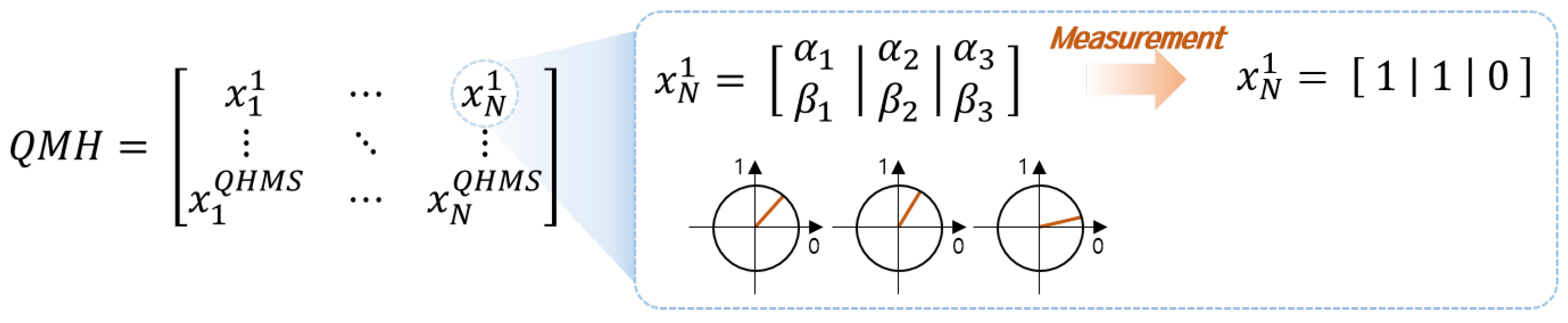
In Step 2, QHM (quantum harmony memory) is initialized, and QHM is configured as shown in Figure 1. Here, N refers to the dimensions of the problem. For example, assuming that there are three qubits, each design variable is expressed as the probability information of qubits. The design variables of the qubit can be expressed as a binary through measurement. Since the information in the qubit consists of probability information, each measurement may have a different value.

Since the QbHS algorithm uses qubits, the process exists only when the initial qubit state is determined. Lee et al. used the QbHS${}_{HG}$ algorithm when the qubit had the same probability of 0 or 1 being selected of 50%, and the QbHS${}_{RV}$ algorithm when the probability of 0 or 1 being selected was random [30]. If the QbHS${}_{RV}$ algorithm is used, it is evaluated once again with the H${}_{ϵ}$ gate. The H${}_{ϵ}$ gate serves to prevent the qubit from fully converging to 0 or 1 in the local minima state, and the convergence of the qubit is prevented by the size of $ϵ$. Equations (4)–(6) are used for the H${}_{ϵ}$ gate. Equations (4) and (6) return the convergence probability to $ϵ$ if ${\left|\alpha \right|}^2$ or ${\left|\beta \right|}^2$ of the qubit converges above $ϵ$.

$${\left[{\alpha }_i{\beta }_i\right]}^T={\left[\sqrt{ϵ}\sqrt{1-ϵ}\right]}^T$$

(4)

$${\left[{\alpha }_i{\beta }_i\right]}^T={\left[\sqrt{1-ϵ}\sqrt{ϵ}\right]}^T$$

(5)

$${\left[{\alpha }_i{\beta }_i\right]}^T={\left[{\alpha }_i{\beta }_i\right]}^T$$

(6)

In Step 3, pitch adjusting is performed in the conventional HS algorithm; this is the most important step that determines the convergence performance of the algorithm. The QbHS algorithm is also performed by pitch adjusting the probabilities of QHMCR and QPAR. Lee et al. proposed performing sound control using the basic qubit state and expressed it as Equation (7) [30]. Here, r is a random number between 0 and 1, and pitch adjusting is performed around the current probability information. $Qbw$ is calculated by Equation (8).

$$\left\{\begin{array}{cc}{\alpha }_i^{t+1}={\left|{\alpha }_i^t\right|}^2+r\times Qbw& r<0.5\\ {\alpha }_i^{t+1}={\left|{\alpha }_i^t\right|}^2-r\times Qbw& else\end{array}\right.$$

(7)

$$Qbw=0.7\times \left(0.9\times qb{w}_{max}\times exp\left(\frac{log\left(\frac{qb{w}_{min}}{qb{w}_{max}}\right)}{0.7}\right)\times \frac{t}{t_{max}}\right)$$

(8)

In addition, the QbHS algorithm was proposed to change the number of qubits that perform pitch adjusting according to the number of generations. Within a certain number of generations, all qubits perform pitch adjusting, but when the probability mean of qubits exceeds $tolBW$, qubits, in addition to BWQ probabilities, are adopted to perform pitch adjusting. These characteristics improve the exploitation performance toward the end of the generation. The qubit performs rotation using the current generation and uses a rotation gate. A rotation gate is defined in Equation (9), and $\theta$ is defined in Equation (10). Here, $\Delta \theta$ is determined using a lookup table, and ${\theta }_r$ is used as a variable.

Table 1. Lookup table for rotation gate.

${\mathit{x}}_{\mathit{i}}$	${\mathit{b}}_{\mathit{i}}$	$\mathit{f}\left(\mathit{x}\right)<\mathit{f}\left(\mathit{b}\right)$	$\mathbf{\Delta }\mathit{\theta }$	$\mathit{s}\mathit{i}\mathit{g}\mathit{n}$(${\mathit{\alpha }}_{\mathit{i}}{\mathit{\beta }}_{\mathit{i}}$)
				${\mathit{\alpha }}_{\mathit{i}}{\mathit{\beta }}_{\mathit{i}}>\mathbf{0}$	${\mathit{\alpha }}_{\mathit{i}}{\mathit{\beta }}_{\mathit{i}}<\mathbf{0}$	${\mathit{\alpha }}_{\mathit{i}}=\mathbf{0}$	${\mathit{\beta }}_{\mathit{i}}=\mathbf{0}$
0	0	True	0	0	0	0	0
0	0	False	0	0	0	0	0
0	1	True	${\theta }_P$	1	−1	0	$\pm 1$
0	1	False	0	0	0	0	0
1	0	True	${\theta }_N$1	1	−1	$\pm 1$	0
1	0	False	0	0	0	0	0
1	1	True	0	0	0	0	0
1	1	False	0	0	0	0	0

¹${\theta }_N=-{\theta }_P$

shows the lookup table.

$$\left\{\begin{array}{c}{\alpha }_i^{t+1}\\ {\beta }_i^{t+1}\end{array}\right\}=\left[\begin{array}{cc}cos\left(\theta \right)& -sin\left(\theta \right)\\ sin\left(\theta \right)& cos\left(\theta \right)\end{array}\right]\left\{\begin{array}{c}{\alpha }_i^t\\ {\beta }_i^t\end{array}\right\}$$

(9)

$$\theta =\Delta \theta \times sign\left({\alpha }_i{\beta }_i\right)$$

(10)

In Step 4, as in the conventional HS algorithm, whether or not to update is determined by comparing the qubit information of the previous generation with the qubit information in which pitch adjusting has been performed in Step 3. Since the QbHS algorithm constructs QHM using the qubit containing probability information, it compares fitness through the measurement of qubits. After comparison, the probability information of the qubit derived from better fitness is updated to the QHM. Through this process, the qubit converges to 0 or 1, and information accumulates.

In Step 5, the algorithm is terminated by the termination condition, and the optimization result is shown. As in the conventional HS algorithm, the QbHS algorithm mainly uses termination conditions using the number of generations. However, the QbHS algorithm can use the new termination condition proposed by Han et al. that uses the convergence of qubits [38], and the new termination condition can be expressed as Equations (11) and (12). Unlike the conventional HS algorithms, the new termination condition uses the convergence of qubits, so the algorithm can be terminated faster, and new results can be derived through measurement.

$$C_b\left(q\right)=\frac{1}{m}\sum _{i=1}^m|1-2|{\alpha }_i{|}^2|\left(\mathrm{or}{C}_b\left(q\right)=\frac{1}{m}\sum _{i=1}^m|1-2|{\beta }_i{|}^2|\right)$$

(11)

$$C_{av}=\left(\frac{1}{N}\sum _{j=1}^N{C}_b\left(q_j\right)\right)>(1-2ϵ)\gamma$$

(12)

3. Characteristics of the QbHS Algorithm

Table 2. Benchmark function for comparison.

Function	Name	Boundary	Min	${\mathit{t}}_{\mathbf{max}}$	Qubit
$f_{01}$	Sphere function	[−100 100]	0	500	18
$f_{02}$	Ackley’s function	[−32 32]	0	800	18
$f_{03}$	Griewank’s function	[−600 600]	0	1000	21
$f_{04}$	Rastrigin’s function	[−5.12 5.12]	0	2000	17
$f_{05}$	Schwefel’s function 2.26	[−500 500]	0	4000	22
$f_{06}$	Rosenbrock’s function	[−30 30]	0	8000	18

shows the benchmark function used to compare the convergence performance according to parameter changes and the number of qubits used in each benchmark function [39,40]. Here, Min is the minimum value of the function, and $t_{max}$ is the maximum number of generations. The parameters selected for the comparison of convergence performance with changes in values are QHMS, QHMCR, QPAR, $ϵ$, and ${\theta }_r$. In addition, among the methods of initializing QHM for convergence performance comparison, the QbHS${}_{RV}$ algorithm, which constructs the initial qubit state as a random number, was used.

3.1. QHMS

HMS (harmony memory size), one of the parameters for constructing HM (harmony memory) in conventional HS algorithms, is one of the parameters sensitive to convergence performance. Therefore, QHMS, with the same role as the HM of conventional HS algorithms, was adopted in QbHS algorithms, and the effect of the QHMS size change on convergence performance was compared.

Table 3. Parameters for QHMS analysis.

d	QHMS	QHMCR	QPAR	$\mathit{ϵ}$	${\mathit{\theta }}_{\mathit{r}}$	Mea.	$\mathit{qbw}$
							tolBW	${\mathit{qbw}}_{\mathit{max}}$	${\mathit{qbw}}_{\mathit{min}}$
20	1–100	0.9	0.1	0.01	0.06	1	0.95	1.0	0.01

presents the parameters for the interpretation of QHMS changes. QHMS was interpreted by changing it to 1, 5, 10, 20, 40, 60, and 100, and other parameters had fixed values. The interpretation was repeated 50 times.

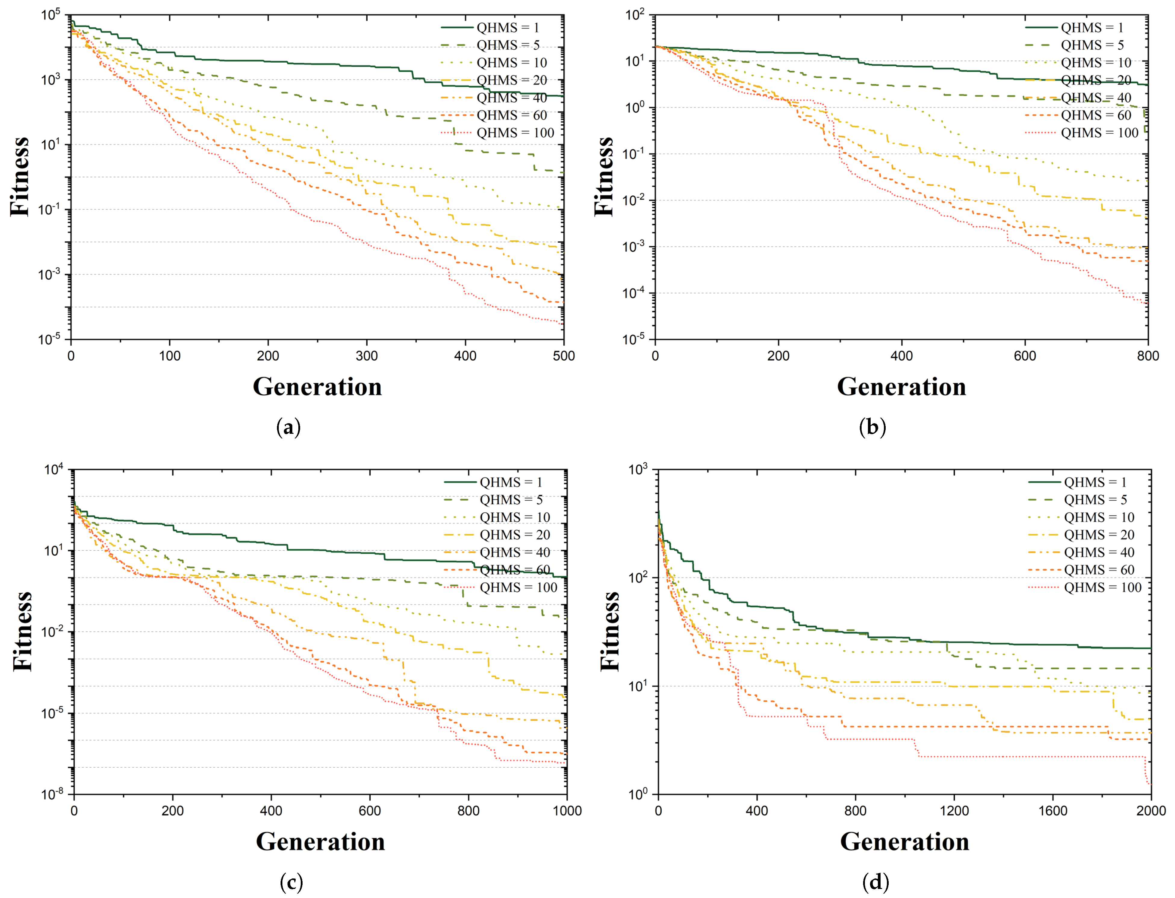
Figure 2 is the convergence graph of best fitness according to the change in QHMS, and the interpretation results are summarized in

Table A1. Benchmark function results according to QHMS.

Funct.	Index	QHMS
		1	5	10	20	40	60	100
$f_{01}$	BF	3.162 $\times {10}^{+2}$	1.387 $\times {10}^0$	1.200 $\times {10}^{-1}$	4.785 $\times {10}^{-3}$	6.863 $\times {10}^{-4}$	1.403 $\times {10}^{-4}$	3.085 $\times {10}^{-5}$
	MF	1.048 $\times {10}^{+3}$	8.719 $\times {10}^0$	8.578 $\times {10}^{-1}$	6.648 $\times {10}^{-2}$	4.966 $\times {10}^{-3}$	1.149 $\times {10}^{-3}$	1.558 $\times {10}^{-4}$
	Std	4.461 $\times {10}^{+2}$	7.235 $\times {10}^0$	8.215 $\times {10}^{-1}$	4.487 $\times {10}^{-2}$	3.712 $\times {10}^{-2}$	7.524 $\times {10}^{-4}$	1.158 $\times {10}^{-4}$
$f_{02}$	BF	3.091 $\times {10}^0$	2.955 $\times {10}^{-1}$	2.507 $\times {10}^{-2}$	4.300 $\times {10}^{-3}$	9.549 $\times {10}^{-4}$	4.891 $\times {10}^{-4}$	6.105 $\times {10}^{-5}$
	MF	5.528 $\times {10}^0$	2.104 $\times {10}^0$	1.706 $\times {10}^0$	1.603 $\times {10}^0$	8.970 $\times {10}^{-1}$	5.772 $\times {10}^{-1}$	1.394 $\times {10}^{-1}$
	Std	1.344 $\times {10}^0$	4.933 $\times {10}^{-1}$	9.041 $\times {10}^{-1}$	8.460 $\times {10}^{-1}$	9.534 $\times {10}^{-1}$	8.727 $\times {10}^{-1}$	4.135 $\times {10}^{-1}$
$f_{03}$	BF	1.076 $\times {10}^0$	2.910 $\times {10}^{-2}$	1.429 $\times {10}^{-3}$	3.956 $\times {10}^{-5}$	2.842 $\times {10}^{-6}$	3.060 $\times {10}^{-7}$	1.477 $\times {10}^{-7}$
	MF	1.849 $\times {10}^0$	2.260 $\times {10}^{-1}$	1.637 $\times {10}^{-1}$	1.112 $\times {10}^{-1}$	7.753 $\times {10}^{-2}$	6.532 $\times {10}^{-2}$	5.948 $\times {10}^{-2}$
	Std	9.218 $\times {10}^{-1}$	1.322 $\times {10}^{-1}$	1.352 $\times {10}^{-1}$	9.429 $\times {10}^{-2}$	9.152 $\times {10}^{-2}$	5.555 $\times {10}^{-2}$	5.274 $\times {10}^{-2}$
$f_{04}$	BF	2.238 $\times {10}^{+1}$	1.460 $\times {10}^{+1}$	8.689 $\times {10}^0$	4.945 $\times {10}^0$	3.709 $\times {10}^0$	3.236 $\times {10}^0$	1.236 $\times {10}^0$
	MF	4.297 $\times {10}^{+1}$	3.006 $\times {10}^{+1}$	2.310 $\times {10}^{+1}$	1.808 $\times {10}^{+1}$	1.499 $\times {10}^{+1}$	1.164 $\times {10}^{+1}$	9.036 $\times {10}^0$
	Std	9.897 $\times {10}^0$	9.566 $\times {10}^0$	6.573 $\times {10}^0$	6.608 $\times {10}^0$	6.888 $\times {10}^0$	5.747 $\times {10}^0$	4.374 $\times {10}^0$
$f_{05}$	BF	4.890 $\times {10}^{+2}$	4.588 $\times {10}^{+2}$	1.719 $\times {10}^{+2}$	3.477 $\times {10}^{+1}$	7.286 $\times {10}^{-1}$	6.248 $\times {10}^{-1}$	4.186 $\times {10}^{-1}$
	MF	1.426 $\times {10}^{+3}$	9.323 $\times {10}^{+2}$	5.291 $\times {10}^{+2}$	2.149 $\times {10}^{+2}$	4.734 $\times {10}^{+1}$	8.553 $\times {10}^0$	1.102 $\times {10}^0$
	Std	3.708 $\times {10}^{+2}$	2.738 $\times {10}^{+2}$	2.615 $\times {10}^{+2}$	1.399 $\times {10}^{+2}$	7.457 $\times {10}^{+1}$	2.469 $\times {10}^{+1}$	2.629 $\times {10}^{-1}$
$f_{06}$	BF	1.772 $\times {10}^{+1}$	1.713 $\times {10}^{+1}$	1.718 $\times {10}^{+1}$	1.638 $\times {10}^{+1}$	1.805 $\times {10}^{+1}$	1.441 $\times {10}^{+1}$	1.617 $\times {10}^{+1}$
	MF	1.944 $\times {10}^{+3}$	3.597 $\times {10}^{+2}$	2.778 $\times {10}^{+2}$	2.087 $\times {10}^{+2}$	1.746 $\times {10}^{+2}$	1.079 $\times {10}^{+2}$	1.080 $\times {10}^{+2}$
	Std	1.051 $\times {10}^{+4}$	5.556 $\times {10}^{+2}$	4.280 $\times {10}^{+2}$	4.588 $\times {10}^{+2}$	3.433 $\times {10}^{+2}$	1.376 $\times {10}^{+2}$	2.186 $\times {10}^{+2}$
Ranking	BF	6.83	5.67	5.00	3.83	3.67	1.83	1.17
	MF	7.00	6.00	5.00	4.00	3.00	1.83	1.17
	AVG(BF, MF)	6.92	5.83	5.00	3.92	3.33	1.83	1.17

. The smaller the size of the QHMS, the closer it was to green, and the larger the size of the QHMS, the closer it was to red. In all six functions, the larger the size of QHMS, the closer the result was to Min, and on the contrary, the smaller the size of QHMS, the farther the result was from Min. In terms of the average value using BF (best fitness) and MF (mean fitness), as presented in Table A1, QHMS was the worst at 6.92 when it had a value of 1 and the best at 1.17 when it had a value of 100.

Therefore, it was confirmed that the larger the QHMS, the better the convergence performance of the QbHS algorithm. This characteristic is because the larger the QHMS, the larger the QHM, so the probability of selecting a better value increases. It is also a characteristic similar to that of the conventional HS algorithms.

3.2. QHMCR and QPAR

The parameters that respond most sensitively to convergence performance in the conventional HS algorithms are known as HMCR and PAR [41]. The convergence performance of the conventional HS algorithms is the best when HMCR has values of 0.7–0.95 and PAR has values of 0.1–0.5. Therefore, the convergence performance of QHMCR and QPAR, which play the same role as HMCR and PAR in the conventional HS algorithms, was compared.

Table 4. Parameters for QHMCR and QPAR analysis.

d	QHMS	QHMCR	QPAR	$\mathit{ϵ}$	${\mathit{\theta }}_{\mathit{r}}$	Mea.	$\mathit{qbw}$
							tolBW	${\mathit{qbw}}_{\mathit{max}}$	${\mathit{qbw}}_{\mathit{min}}$
20	10	0.1–0.9	0.1–0.9	0.01	0.06	8	0.95	1.0	0.01

is a parameter for the interpretation of QHMCR and QPAR changes. QHMCR and QPAR were changed to 0.1, 0.3, 0.5, 0.7, and 0.9, respectively, and other parameters were fixed. The interpretation was repeated 50 times.

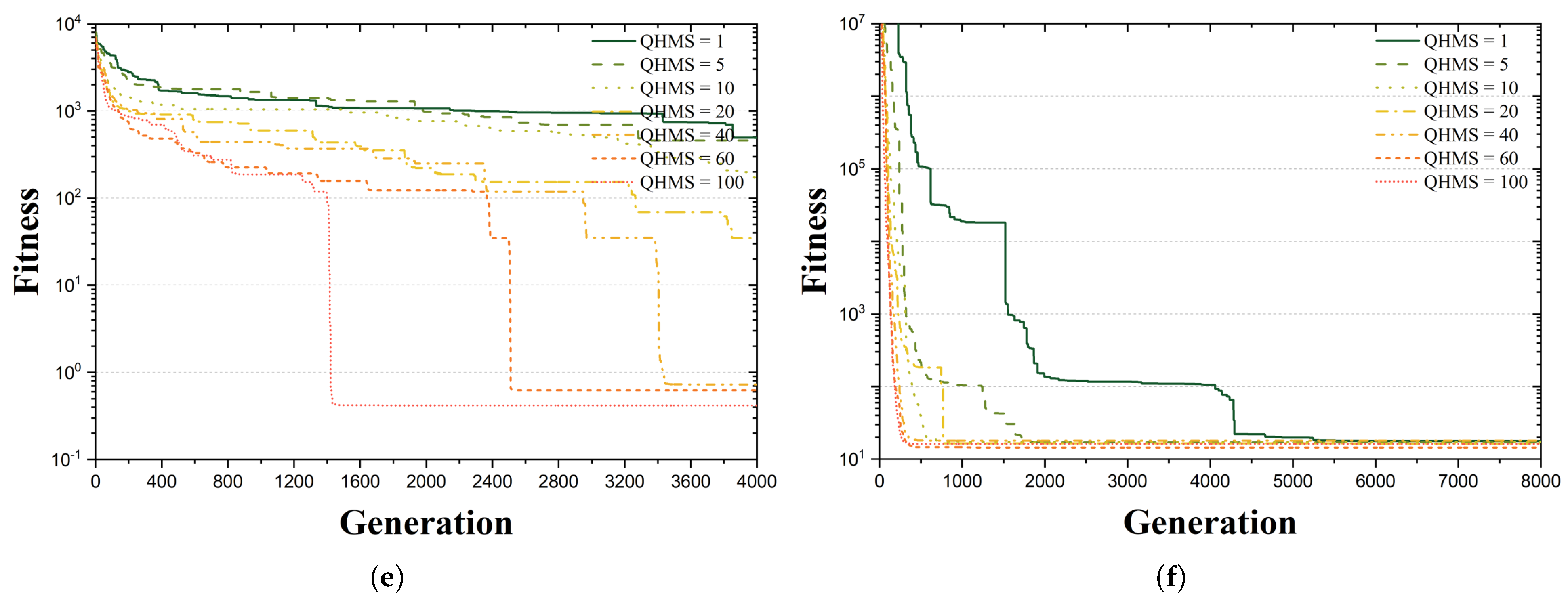
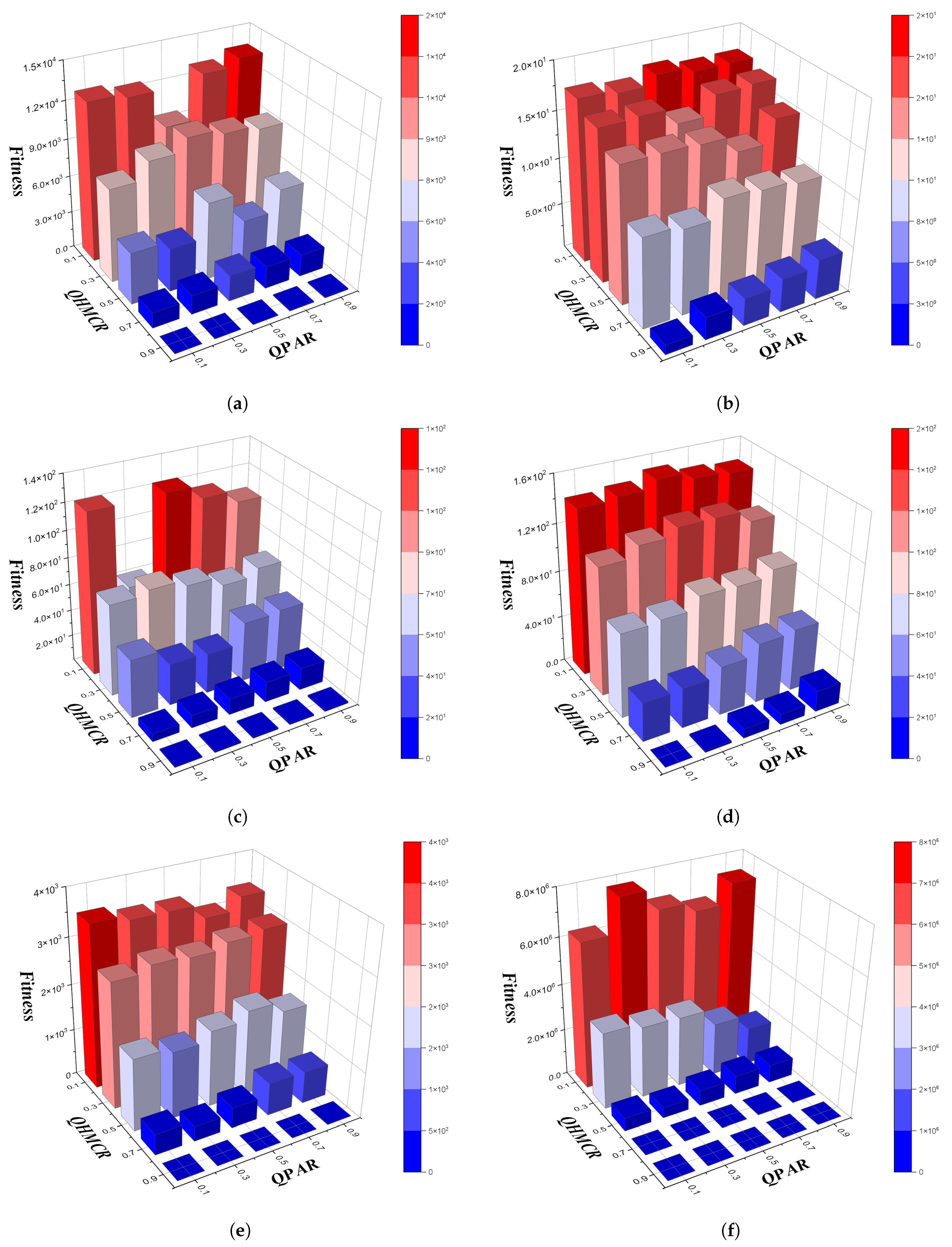
Figure 3 is a 3D bar graph expressing the analysis results of each benchmark function, and the analysis results are summarized in

Table A2. Benchmark function results according to QHMCR and QPAR.

Funct.	QPAR	Index	QHMCR
			0.1	0.3	0.5	0.7	0.9
$f_{01}$	0.1	BF	1.279 $\times {10}^{+4}$	7.571 $\times {10}^{+3}$	4.188 $\times {10}^{+3}$	1.260 $\times {10}^{+3}$	5.714 $\times {10}^0$
		MF	1.864 $\times {10}^{+4}$	1.354 $\times {10}^{+4}$	8.048 $\times {10}^{+3}$	2.544 $\times {10}^{+3}$	2.023 $\times {10}^{+1}$
		Std	2.287 $\times {10}^{+3}$	2.652 $\times {10}^{+3}$	1.555 $\times {10}^{+3}$	6.756 $\times {10}^{+2}$	1.119 $\times {10}^{+1}$
	0.3	BF	1.245 $\times {10}^{+4}$	8.951 $\times {10}^{+3}$	3.540 $\times {10}^{+3}$	1.561 $\times {10}^{+3}$	1.495 $\times {10}^{+1}$
		MF	1.853 $\times {10}^{+4}$	1.376 $\times {10}^{+4}$	8.812 $\times {10}^{+3}$	2.765 $\times {10}^{+3}$	4.104 $\times {10}^{+1}$
		Std	2.044 $\times {10}^{+3}$	1.959 $\times {10}^{+3}$	1.616 $\times {10}^{+3}$	6.516 $\times {10}^{+2}$	1.846 $\times {10}^{+1}$
	0.5	BF	9.470 $\times {10}^{+3}$	9.985 $\times {10}^{+3}$	6.326 $\times {10}^{+3}$	2.109 $\times {10}^{+3}$	3.052 $\times {10}^{+1}$
		MF	1.871 $\times {10}^{+4}$	1.425 $\times {10}^{+4}$	8.938 $\times {10}^{+3}$	3.252 $\times {10}^{+3}$	8.475 $\times {10}^{+1}$
		Std	2.794 $\times {10}^{+3}$	1.942 $\times {10}^{+3}$	1.304 $\times {10}^{+3}$	7.582 $\times {10}^{+2}$	3.833 $\times {10}^{+1}$
	0.7	BF	1.295 $\times {10}^{+4}$	9.541 $\times {10}^{+3}$	3.935 $\times {10}^{+3}$	1.832 $\times {10}^{+3}$	8.140 $\times {10}^{+1}$
		MF	1.905 $\times {10}^{+4}$	1.423 $\times {10}^{+4}$	8.885 $\times {10}^{+3}$	3.340 $\times {10}^{+3}$	1.614 $\times {10}^{+2}$
		Std	2.719 $\times {10}^{+3}$	1.990 $\times {10}^{+3}$	1.583 $\times {10}^{+3}$	8.188 $\times {10}^{+2}$	4.966 $\times {10}^{+1}$
	0.9	BF	1.360 $\times {10}^{+4}$	9.186 $\times {10}^{+3}$	5.664 $\times {10}^{+3}$	1.823 $\times {10}^{+3}$	1.035 $\times {10}^{+2}$
		MF	1.878 $\times {10}^{+4}$	1.409 $\times {10}^{+4}$	8.785 $\times {10}^{+3}$	3.822 $\times {10}^{+3}$	2.707 $\times {10}^{+2}$
		Std	2.301 $\times {10}^{+3}$	1.856 $\times {10}^{+3}$	1.438 $\times {10}^{+3}$	9.882 $\times {10}^{+2}$	8.303 $\times {10}^{+1}$
$f_{02}$	0.1	BF	1.739 $\times {10}^{+1}$	1.628 $\times {10}^{+1}$	1.464 $\times {10}^{+1}$	9.621 $\times {10}^0$	1.030 $\times {10}^0$
		MF	1.875 $\times {10}^{+1}$	1.782 $\times {10}^{+1}$	1.604 $\times {10}^{+1}$	1.163 $\times {10}^{+1}$	2.542 $\times {10}^0$
		Std	3.967 $\times {10}^{+1}$	4.695 $\times {10}^{-1}$	6.112 $\times {10}^{-1}$	8.795 $\times {10}^{-1}$	4.854 $\times {10}^{-1}$
	0.3	BF	1.706 $\times {10}^{+1}$	1.644 $\times {10}^{+1}$	1.465 $\times {10}^{+1}$	9.175 $\times {10}^0$	2.442 $\times {10}^0$
		MF	1.872 $\times {10}^{+1}$	1.796 $\times {10}^{+1}$	1.609 $\times {10}^{+1}$	1.200 $\times {10}^{+1}$	3.238 $\times {10}^0$
		Std	4.467 $\times {10}^{-1}$	4.182 $\times {10}^{-1}$	6.520 $\times {10}^{-1}$	1.126 $\times {10}^0$	4.882 $\times {10}^{-1}$
	0.5	BF	1.802 $\times {10}^{+1}$	1.477 $\times {10}^{+1}$	1.448 $\times {10}^{+1}$	1.107 $\times {10}^{+1}$	2.950 $\times {10}^0$
		MF	1.874 $\times {10}^{+1}$	1.781 $\times {10}^{+1}$	1.611 $\times {10}^{+1}$	1.245 $\times {10}^{+1}$	3.908 $\times {10}^0$
		Std	3.539 $\times {10}^{-1}$	6.198 $\times {10}^{-1}$	7.660 $\times {10}^{-1}$	8.004 $\times {10}^{-1}$	5.072 $\times {10}^{-1}$
	0.7	BF	1.755 $\times {10}^{+1}$	1.679 $\times {10}^{+1}$	1.274 $\times {10}^{+1}$	1.075 $\times {10}^{+1}$	3.618 $\times {10}^0$
		MF	1.873 $\times {10}^{+1}$	1.788 $\times {10}^{+1}$	1.615 $\times {10}^{+1}$	1.286 $\times {10}^{+1}$	4.864 $\times {10}^0$
		Std	3.785 $\times {10}^{-1}$	4.855 $\times {10}^{-1}$	9.103 $\times {10}^{-1}$	8.175 $\times {10}^{-1}$	5.925 $\times {10}^{-1}$
	0.9	BF	1.760 $\times {10}^{+1}$	1.698 $\times {10}^{+1}$	1.510 $\times {10}^{+1}$	1.035 $\times {10}^{+1}$	4.313 $\times {10}^0$
		MF	1.867 $\times {10}^{+1}$	1.794 $\times {10}^{+1}$	1.650 $\times {10}^{+1}$	1.314 $\times {10}^{+1}$	5.716 $\times {10}^0$
		Std	3.507 $\times {10}^{-1}$	4.265 $\times {10}^{-1}$	6.957 $\times {10}^{-1}$	9.032 $\times {10}^{-1}$	7.792 $\times {10}^{-1}$
$f_{03}$	0.1	BF	1.218 $\times {10}^{+2}$	6.916 $\times {10}^{+1}$	4.396 $\times {10}^{+1}$	6.147 $\times {10}^0$	7.966 $\times {10}^{-1}$
		MF	1.592 $\times {10}^{+2}$	1.148 $\times {10}^{+2}$	6.585 $\times {10}^{+1}$	1.835 $\times {10}^{+1}$	1.038 $\times {10}^0$
		Std	1.866 $\times {10}^{+1}$	1.932 $\times {10}^{+1}$	9.703 $\times {10}^0$	5.688 $\times {10}^0$	5.307 $\times {10}^{-2}$
	0.3	BF	6.040 $\times {10}^{+1}$	7.250 $\times {10}^{+1}$	3.162 $\times {10}^{+1}$	9.727 $\times {10}^0$	1.021 $\times {10}^0$
		MF	1.586 $\times {10}^{+2}$	1.168 $\times {10}^{+2}$	6.771 $\times {10}^{+1}$	1.983 $\times {10}^{+1}$	1.082 $\times {10}^0$
		Std	2.277 $\times {10}^{+1}$	1.526 $\times {10}^{+1}$	1.238 $\times {10}^{+1}$	5.482 $\times {10}^0$	3.705 $\times {10}^{-2}$
	0.5	BF	1.227 $\times {10}^{+2}$	6.784 $\times {10}^{+1}$	3.018 $\times {10}^{+1}$	1.224 $\times {10}^{+1}$	1.048 $\times {10}^0$
		MF	1.649 $\times {10}^{+2}$	1.159 $\times {10}^{+2}$	7.145 $\times {10}^{+1}$	2.244 $\times {10}^{+1}$	1.209 $\times {10}^0$
		Std	1.672 $\times {10}^{+1}$	1.769 $\times {10}^{+1}$	1.523 $\times {10}^{+1}$	5.062 $\times {10}^0$	1.118 $\times {10}^{-1}$
	0.7	BF	1.129 $\times {10}^{+2}$	6.054 $\times {10}^{+1}$	4.580 $\times {10}^{+1}$	1.551 $\times {10}^{+1}$	1.138 $\times {10}^0$
		MF	1.601 $\times {10}^{+2}$	1.146 $\times {10}^{+2}$	7.000 $\times {10}^{+1}$	2.532 $\times {10}^{+1}$	1.499 $\times {10}^0$
		Std	1.996 $\times {10}^{+1}$	1.869 $\times {10}^{+1}$	1.237 $\times {10}^{+1}$	5.446 $\times {10}^0$	2.556 $\times {10}^{-1}$
	0.9	BF	1.042 $\times {10}^{+2}$	6.623 $\times {10}^{+1}$	4.747 $\times {10}^{+1}$	1.716 $\times {10}^{+1}$	1.266 $\times {10}^0$
		MF	1.626 $\times {10}^{+2}$	1.216 $\times {10}^{+2}$	7.440 $\times {10}^{+1}$	2.787 $\times {10}^{+1}$	1.831 $\times {10}^0$
		Std	2.052 $\times {10}^{+1}$	1.931 $\times {10}^{+1}$	1.325 $\times {10}^{+1}$	6.395 $\times {10}^0$	3.024 $\times {10}^{-1}$
$f_{04}$	0.1	BF	1.416 $\times {10}^{+2}$	1.098 $\times {10}^{+2}$	7.243 $\times {10}^{+1}$	3.336 $\times {10}^{+1}$	6.330 $\times {10}^{-3}$
		MF	1.708 $\times {10}^{+2}$	1.421 $\times {10}^{+2}$	9.851 $\times {10}^{+1}$	4.619 $\times {10}^{+1}$	9.242 $\times {10}^{-1}$
		Std	1.129 $\times {10}^{+1}$	9.687 $\times {10}^0$	9.558 $\times {10}^0$	7.032 $\times {10}^0$	9.045 $\times {10}^{-1}$
	0.3	BF	1.440 $\times {10}^{+2}$	1.190 $\times {10}^{+2}$	7.421 $\times {10}^{+1}$	3.444 $\times {10}^{+1}$	1.637 $\times {10}^0$
		MF	1.753 $\times {10}^{+2}$	1.436 $\times {10}^{+2}$	1.034 $\times {10}^{+2}$	5.306 $\times {10}^{+1}$	5.301 $\times {10}^0$
		Std	9.039 $\times {10}^0$	1.069 $\times {10}^{+1}$	9.931 $\times {10}^0$	7.812 $\times {10}^0$	1.853 $\times {10}^0$
	0.5	BF	1.510 $\times {10}^{+2}$	1.257 $\times {10}^{+2}$	8.469 $\times {10}^{+1}$	4.214 $\times {10}^{+1}$	8.086 $\times {10}^0$
		MF	1.731 $\times {10}^{+2}$	1.460 $\times {10}^{+2}$	1.051 $\times {10}^{+2}$	5.907 $\times {10}^{+1}$	1.176 $\times {10}^{+1}$
		Std	9.748 $\times {10}^0$	9.287 $\times {10}^0$	9.593 $\times {10}^0$	8.551 $\times {10}^0$	2.495 $\times {10}^0$
	0.7	BF	1.451 $\times {10}^{+2}$	1.256 $\times {10}^{+2}$	8.393 $\times {10}^{+1}$	5.166 $\times {10}^{+1}$	9.087 $\times {10}^0$
		MF	1.748 $\times {10}^{+2}$	1.461 $\times {10}^{+2}$	1.123 $\times {10}^{+2}$	6.500 $\times {10}^0$	2.147 $\times {10}^{+1}$
		Std	1.244 $\times {10}^{+1}$	1.017 $\times {10}^{+1}$	1.153 $\times {10}^{+1}$	9.367 $\times {10}^0$	4.274 $\times {10}^0$
	0.9	BF	1.432 $\times {10}^{+2}$	1.157 $\times {10}^{+2}$	8.962 $\times {10}^{+1}$	5.383 $\times {10}^{+1}$	1.825 $\times {10}^{+1}$
		MF	1.769 $\times {10}^{+2}$	1.491 $\times {10}^{+2}$	1.131 $\times {10}^{+2}$	7.220 $\times {10}^{+1}$	3.194 $\times {10}^{+1}$
		Std	1.037 $\times {10}^{+1}$	1.025 $\times {10}^{+1}$	1.109 $\times {10}^{+1}$	9.904 $\times {10}^0$	5.732 $\times {10}^0$
$f_{05}$	0.1	BF	3.511 $\times {10}^{+3}$	2.715 $\times {10}^{+3}$	1.553 $\times {10}^{+3}$	4.516 $\times {10}^{+2}$	2.155 $\times {10}^{-1}$
		MF	4.245 $\times {10}^{+3}$	3.400 $\times {10}^{+3}$	2.196 $\times {10}^{+3}$	7.358 $\times {10}^{+2}$	6.138 $\times {10}^{-1}$
		Std	2.498 $\times {10}^{+2}$	2.479 $\times {10}^{+2}$	2.562 $\times {10}^{+2}$	1.514 $\times {10}^{+2}$	2.722 $\times {10}^{-1}$
	0.3	BF	3.402 $\times {10}^{+3}$	2.852 $\times {10}^{+3}$	1.445 $\times {10}^{+3}$	3.188 $\times {10}^{+2}$	3.710 $\times {10}^{-1}$
		MF	4.280 $\times {10}^{+3}$	3.439 $\times {10}^{+3}$	2.285 $\times {10}^{+3}$	8.625 $\times {10}^{+2}$	9.603 $\times {10}^{-1}$
		Std	2.432 $\times {10}^{+2}$	2.064 $\times {10}^{+2}$	2.861 $\times {10}^{+2}$	1.973 $\times {10}^{+2}$	2.974 $\times {10}^{-1}$
	0.5	BF	3.396 $\times {10}^{+3}$	2.796 $\times {10}^{+3}$	1.652 $\times {10}^{+3}$	4.463 $\times {10}^{+2}$	7.093 $\times {10}^{-1}$
		MF	4.312 $\times {10}^{+3}$	3.439 $\times {10}^{+3}$	2.376 $\times {10}^{+3}$	9.559 $\times {10}^{+2}$	1.708 $\times {10}^0$
		Std	2.443 $\times {10}^{+2}$	1.949 $\times {10}^{+2}$	2.522 $\times {10}^{+2}$	2.075 $\times {10}^{+2}$	9.339 $\times {10}^{-1}$
	0.7	BF	3.094 $\times {10}^{+3}$	2.923 $\times {10}^{+3}$	1.855 $\times {10}^{+3}$	7.097 $\times {10}^{+2}$	2.129 $\times {10}^0$
		MF	4.239 $\times {10}^{+3}$	3.516 $\times {10}^{+3}$	2.442 $\times {10}^{+3}$	1.096 $\times {10}^{+3}$	1.369 $\times {10}^{+1}$
		Std	2.796 $\times {10}^{+2}$	2.477 $\times {10}^{+2}$	2.275 $\times {10}^{+2}$	1.950 $\times {10}^{+2}$	1.450 $\times {10}^{+1}$
	0.9	BF	3.374 $\times {10}^{+3}$	3.012 $\times {10}^{+3}$	1.615 $\times {10}^{+3}$	6.972 $\times {10}^{+2}$	9.921 $\times {10}^0$
		MF	4.277 $\times {10}^{+3}$	3.539 $\times {10}^{+3}$	2.490 $\times {10}^{+3}$	1.248 $\times {10}^{+3}$	6.615 $\times {10}^{+1}$
		Std	2.328 $\times {10}^{+2}$	2.200 $\times {10}^{+2}$	2.551 $\times {10}^{+2}$	2.397 $\times {10}^{+2}$	4.256 $\times {10}^{+1}$
$f_{06}$	0.1	BF	6.279 $\times {10}^{+6}$	3.299 $\times {10}^{+6}$	5.584 $\times {10}^{+5}$	4.194 $\times {10}^{+3}$	7.815 $\times {10}^0$
		MF	1.556 $\times {10}^{+7}$	6.417 $\times {10}^{+6}$	1.232 $\times {10}^{+6}$	1.160 $\times {10}^{+4}$	7.341 $\times {10}^{+1}$
		Std	3.617 $\times {10}^{+6}$	1.836 $\times {10}^{+6}$	3.954 $\times {10}^{+5}$	6.609 $\times {10}^{+3}$	4.125 $\times {10}^{+1}$
	0.3	BF	7.724 $\times {10}^{+6}$	3.085 $\times {10}^{+6}$	4.562 $\times {10}^{+5}$	2.498 $\times {10}^{+3}$	1.222 $\times {10}^{+1}$
		MF	1.647 $\times {10}^{+7}$	6.917 $\times {10}^{+6}$	1.353 $\times {10}^{+6}$	2.014 $\times {10}^{+4}$	9.499 $\times {10}^{+1}$
		Std	4.446 $\times {10}^{+6}$	1.905 $\times {10}^{+6}$	3.870 $\times {10}^{+5}$	1.307 $\times {10}^{+4}$	8.885 $\times {10}^{+1}$
	0.5	BF	6.871 $\times {10}^{+6}$	3.031 $\times {10}^{+6}$	6.777 $\times {10}^{+5}$	8.852 $\times {10}^{+3}$	1.792 $\times {10}^{+1}$
		MF	1.573 $\times {10}^{+7}$	7.109 $\times {10}^{+6}$	1.479 $\times {10}^{+6}$	2.865 $\times {10}^{+4}$	1.455 $\times {10}^{+2}$
		Std	4.255 $\times {10}^{+6}$	1.911 $\times {10}^{+6}$	4.602 $\times {10}^{+5}$	1.583 $\times {10}^{+4}$	1.259 $\times {10}^{+2}$
	0.7	BF	6.470 $\times {10}^{+6}$	2.280 $\times {10}^{+6}$	8.091 $\times {10}^{+5}$	1.692 $\times {10}^{+4}$	2.201 $\times {10}^{+1}$
		MF	1.706 $\times {10}^{+7}$	6.661 $\times {10}^{+6}$	1.712 $\times {10}^{+6}$	4.240 $\times {10}^{+4}$	1.425 $\times {10}^{+2}$
		Std	4.091 $\times {10}^{+6}$	1.997 $\times {10}^{+6}$	6.701 $\times {10}^{+5}$	2.043 $\times {10}^{+4}$	1.204 $\times {10}^{+2}$
	0.9	BF	7.309 $\times {10}^{+6}$	1.616 $\times {10}^{+6}$	7.881 $\times {10}^{+5}$	1.734 $\times {10}^{+4}$	3.822 $\times {10}^{+1}$
		MF	1.508 $\times {10}^{+7}$	7.260 $\times {10}^{+6}$	1.856 $\times {10}^{+6}$	6.825 $\times {10}^{+4}$	2.557 $\times {10}^{+2}$
		Std	3.890 $\times {10}^{+6}$	2.255 $\times {10}^{+6}$	6.431 $\times {10}^{+5}$	3.201 $\times {10}^{+4}$	2.838 $\times {10}^{+2}$

. In Figure 3, the closer to Min, the more blue, and the further away from Min, the more red. First, checking the change in QHMCR, the closer the value of QHMCR is to 0.9, the more blue it becomes. This characteristic means that it has a value close to Min, especially when it has a range of 0.7 to 0.9, where it has the closest value to Min. Second, the closer QPAR is to 0.1, the closer it is to Min. However, when QHMCR has a value close to 0.1, the effect on the change in QPAR does not occur clearly. That is, changes in QHMCR more dominantly affect convergence performance than do changes in QPAR.

Therefore, the closer QHMCR is to 1, the closer QPAR is to 0, and the better the convergence performance. These characteristics of the QbHS algorithm are similar to the range of HMCR and PAR, which are commonly used in the conventional HS algorithm.

3.3. $ϵ$

$ϵ$ is a parameter used for the $H_{ϵ}$ gate, which prevents the qubit from fully converging to 0 or 1. That is, the smaller the value of $ϵ$, the closer the convergence of the qubit to 0 or 1, and the larger the value, the less the qubit converges. The values of $ϵ$ changed to 0.00, 0.005, 0.01, 0.015, 0.02, and 0.03, and other parameters were used, as presented in

Table 5. Parameters for $ϵ$ analysis.

d	QHMS	QHMCR	QPAR	$\mathit{ϵ}$	${\mathit{\theta }}_{\mathit{r}}$	Mea.	$\mathit{qbw}$
							tolBW	${\mathit{qbw}}_{\mathit{max}}$	${\mathit{qbw}}_{\mathit{min}}$
20	10	0.9	0.1	0.00–0.03	0.06	1	0.95	1.0	0.01

. The interpretation was repeated 50 times.

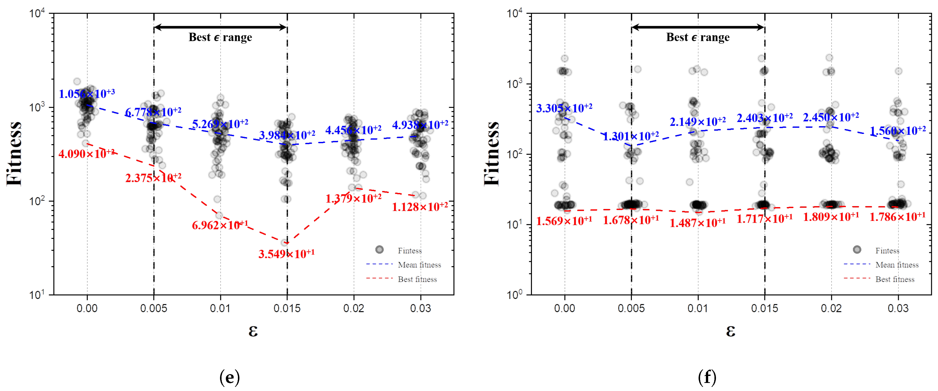
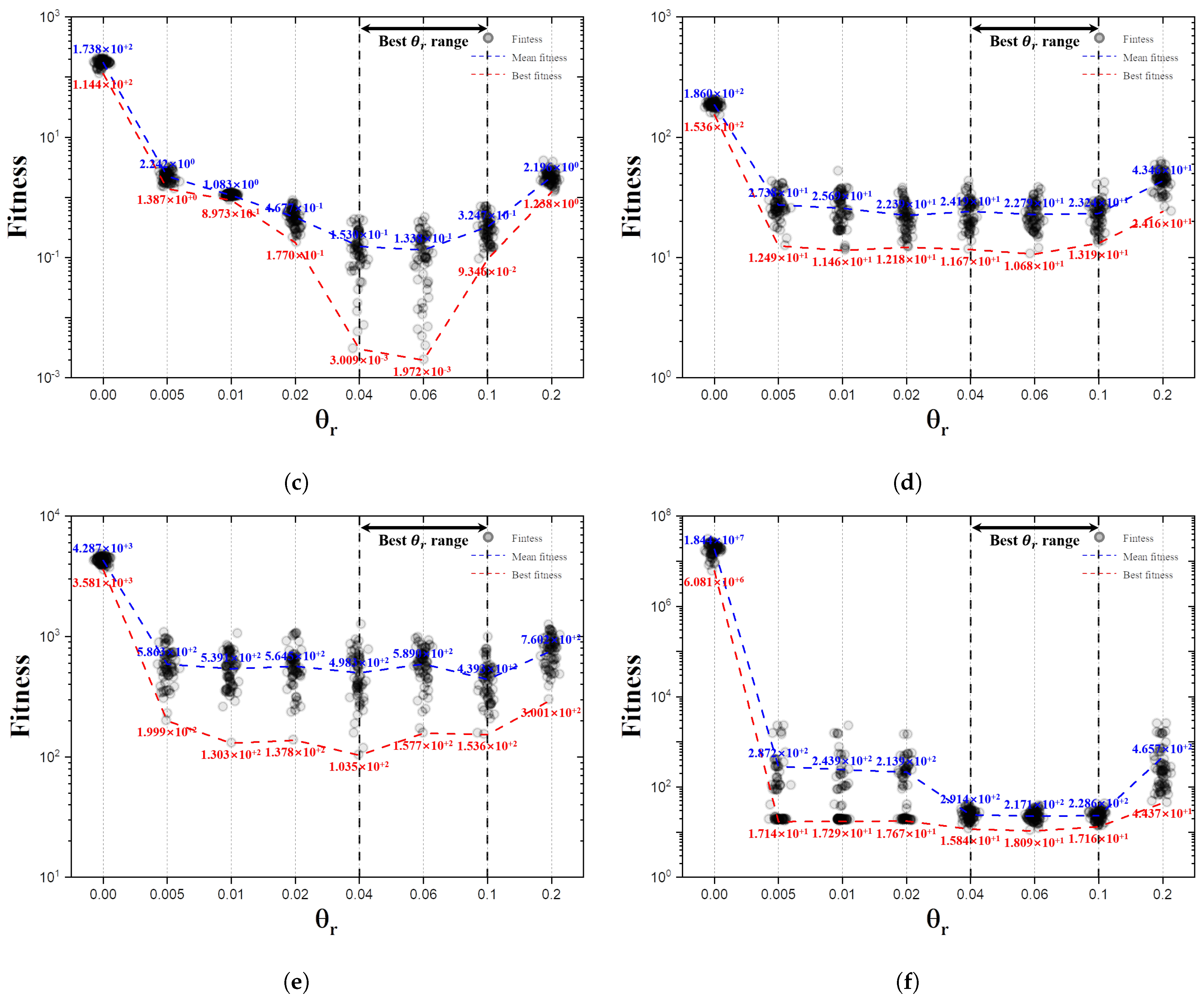
Figure 4 shows the best or mean fitness according to the change in $ϵ$, and the analysis results are summarized in

Table A3. Benchmark function results according to $ϵ$.

Funct.	Index	$\mathit{ϵ}$
		0.000	0.005	0.010	0.015	0.020	0.030
$f_{01}$	BF	7.217 $\times {10}^{-2}$	8.412 $\times {10}^{-2}$	1.303 $\times {10}^{-1}$	3.919 $\times {10}^{-1}$	1.058 $\times {10}^0$	1.546 $\times {10}^{+1}$
	MF	1.536 $\times {10}^{+1}$	5.910 $\times {10}^{-1}$	8.094 $\times {10}^{-1}$	1.843 $\times {10}^0$	7.131 $\times {10}^0$	4.015 $\times {10}^{+1}$
	Std	8.826 $\times {10}^{+1}$	4.960 $\times {10}^{-1}$	6.828 $\times {10}^{-1}$	1.230 $\times {10}^0$	4.676 $\times {10}^0$	2.086 $\times {10}^{+1}$
$f_{02}$	BF	6.849 $\times {10}^{-2}$	1.067 $\times {10}^{-2}$	1.778 $\times {10}^{-2}$	8.569 $\times {10}^{-2}$	2.483 $\times {10}^{-1}$	1.519 $\times {10}^0$
	MF	2.260 $\times {10}^0$	2.034 $\times {10}^0$	1.636 $\times {10}^0$	1.606 $\times {10}^0$	1.837 $\times {10}^0$	2.422 $\times {10}^0$
	Std	4.630 $\times {10}^{-1}$	5.163 $\times {10}^{-1}$	9.638 $\times {10}^{-1}$	8.638 $\times {10}^{-1}$	7.380 $\times {10}^{-1}$	3.304 $\times {10}^{-1}$
$f_{03}$	BF	5.667 $\times {10}^{-5}$	3.471 $\times {10}^{-4}$	1.427 $\times {10}^{-3}$	3.185 $\times {10}^{-2}$	1.675 $\times {10}^{-1}$	1.001 $\times {10}^0$
	MF	2.037 $\times {10}^{-1}$	1.398 $\times {10}^{-1}$	1.408 $\times {10}^{-1}$	1.760 $\times {10}^{-1}$	5.378 $\times {10}^{-1}$	1.051 $\times {10}^0$
	Std	1.530 $\times {10}^{-1}$	1.202 $\times {10}^{-1}$	1.214 $\times {10}^{-1}$	1.150 $\times {10}^{-1}$	1.671 $\times {10}^{-1}$	1.959 $\times {10}^{-2}$
$f_{04}$	BF	1.017 $\times {10}^{+1}$	6.538 $\times {10}^0$	8.177 $\times {10}^0$	1.316 $\times {10}^{+1}$	8.749 $\times {10}^0$	1.613 $\times {10}^{+1}$
	MF	3.558 $\times {10}^{+1}$	2.621 $\times {10}^{+1}$	2.274 $\times {10}^{+1}$	2.235 $\times {10}^{+1}$	2.176 $\times {10}^{+1}$	2.835 $\times {10}^{+1}$
	Std	1.001 $\times {10}^{+1}$	7.451 $\times {10}^0$	6.573 $\times {10}^0$	7.118 $\times {10}^0$	7.489 $\times {10}^0$	6.294 $\times {10}^0$
$f_{05}$	BF	4.090 $\times {10}^{+2}$	2.375 $\times {10}^{+2}$	6.962 $\times {10}^{+1}$	3.549 $\times {10}^{+1}$	1.379 $\times {10}^{+2}$	1.128 $\times {10}^{+2}$
	MF	1.056 $\times {10}^{+3}$	6.778 $\times {10}^{+2}$	5.269 $\times {10}^{+2}$	3.984 $\times {10}^{+2}$	4.456 $\times {10}^{+2}$	4.938 $\times {10}^{+2}$
	Std	3.048 $\times {10}^{+2}$	2.705 $\times {10}^{+2}$	2.587 $\times {10}^{+2}$	1.790 $\times {10}^{+2}$	1.697 $\times {10}^{+2}$	2.098 $\times {10}^{+2}$
$f_{06}$	BF	1.569 $\times {10}^{+1}$	1.678 $\times {10}^{+1}$	1.487 $\times {10}^{+1}$	1.717 $\times {10}^{+1}$	1.809 $\times {10}^{+1}$	1.786 $\times {10}^{+1}$
	MF	3.305 $\times {10}^{+2}$	1.301 $\times {10}^{+2}$	2.149 $\times {10}^{+2}$	2.403 $\times {10}^{+2}$	2.450 $\times {10}^{+2}$	1.560 $\times {10}^{+2}$
	Std	5.148 $\times {10}^{+2}$	2.575 $\times {10}^{+2}$	3.705 $\times {10}^{+2}$	4.587 $\times {10}^{+2}$	4.609 $\times {10}^{+2}$	2.434 $\times {10}^{+2}$
Ranking	BF	2.83	2.33	2.17	3.67	4.67	5.33
	MF	5.33	2.67	2.67	2.33	3.33	4.67
	AVG(BF, MF)	4.08	2.50	2.42	3.00	4.00	5.00

. The gray circles in Figure 4 are the results of a single analysis, and there are 50 gray circles depending on the size of $ϵ$. The red line means the best fitness, and the blue line means the mean fitness among 50 analyses. Checking the red lines, $f_{01}$ and $f_{03}$ were closest to Min when $ϵ$ was 0.000, and $f_{02}$ and $f_{04}$ were closest to Min when $ϵ$ was 0.005. However, if $ϵ$ is 0.000, it is difficult to proactively escape from many problems with local minima. Therefore, 0.000 was excluded from the best $ϵ$ range. In the average ranking using BF and MF, as shown in Table A3, it can be seen that the convergence performance is the best when $ϵ$ is 0.005–0.015.

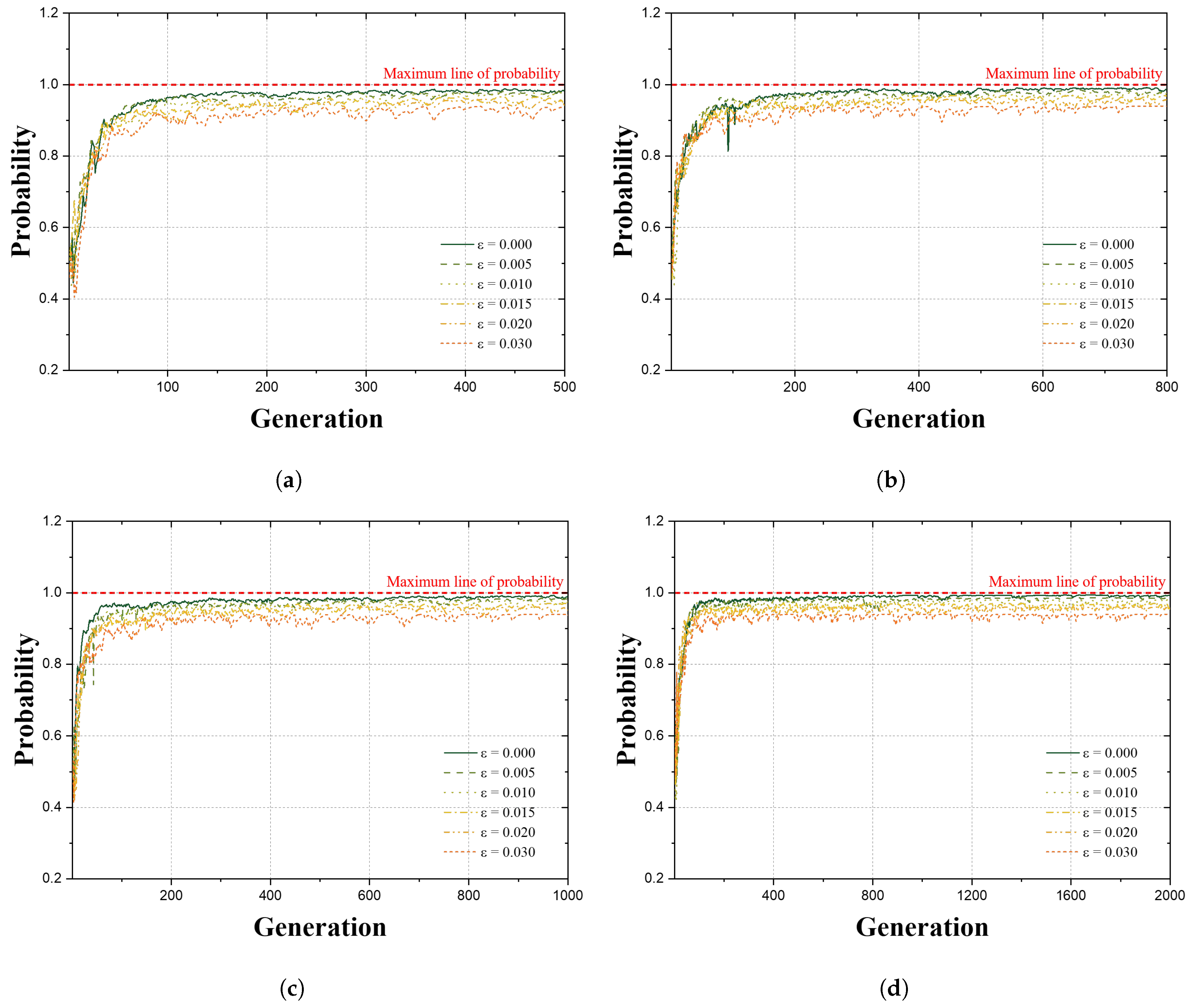
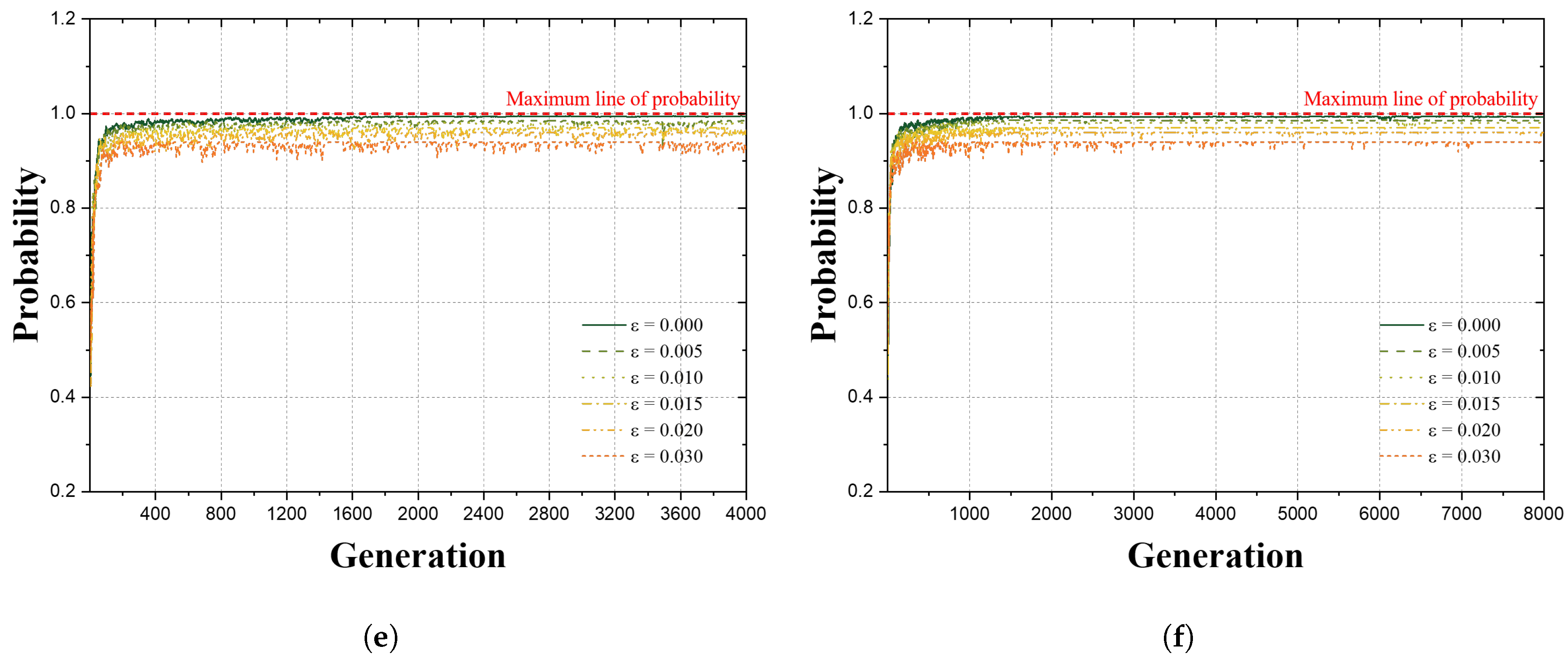
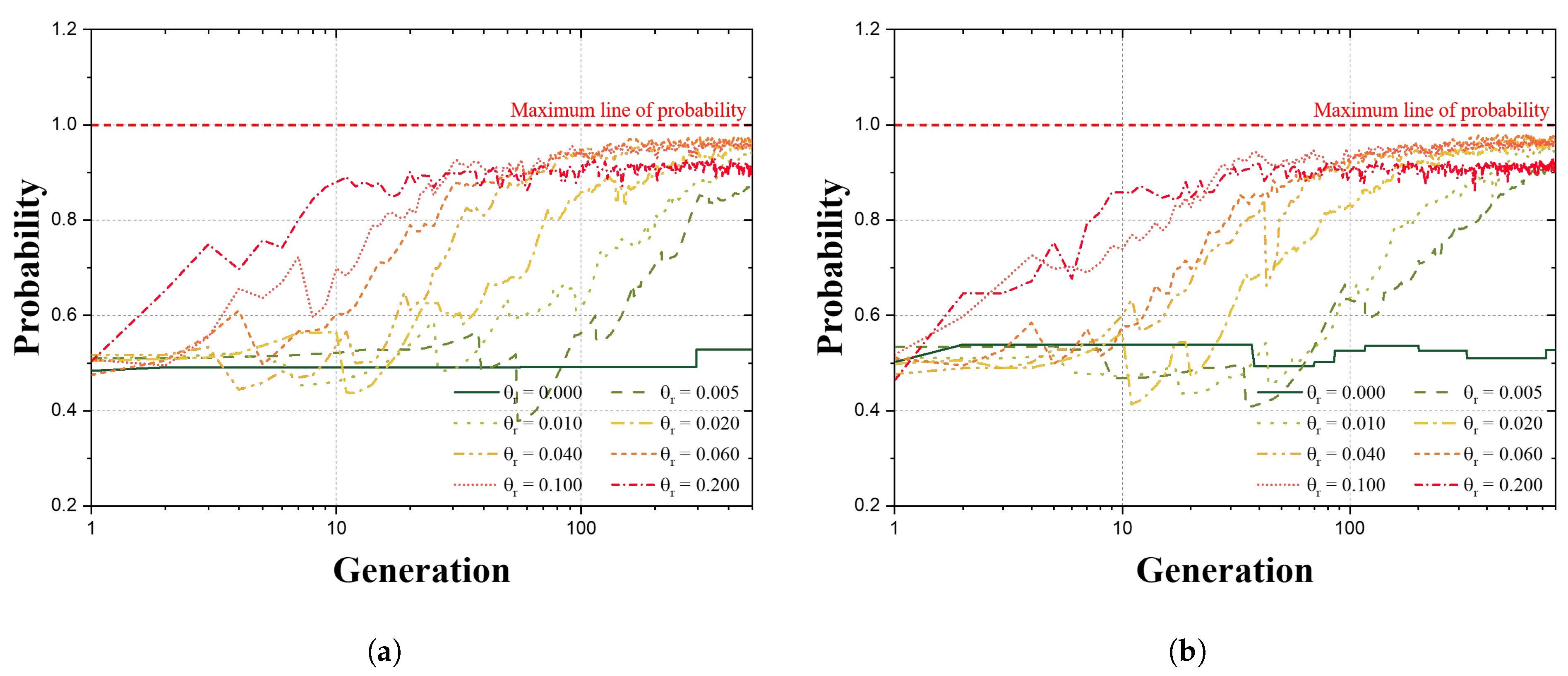
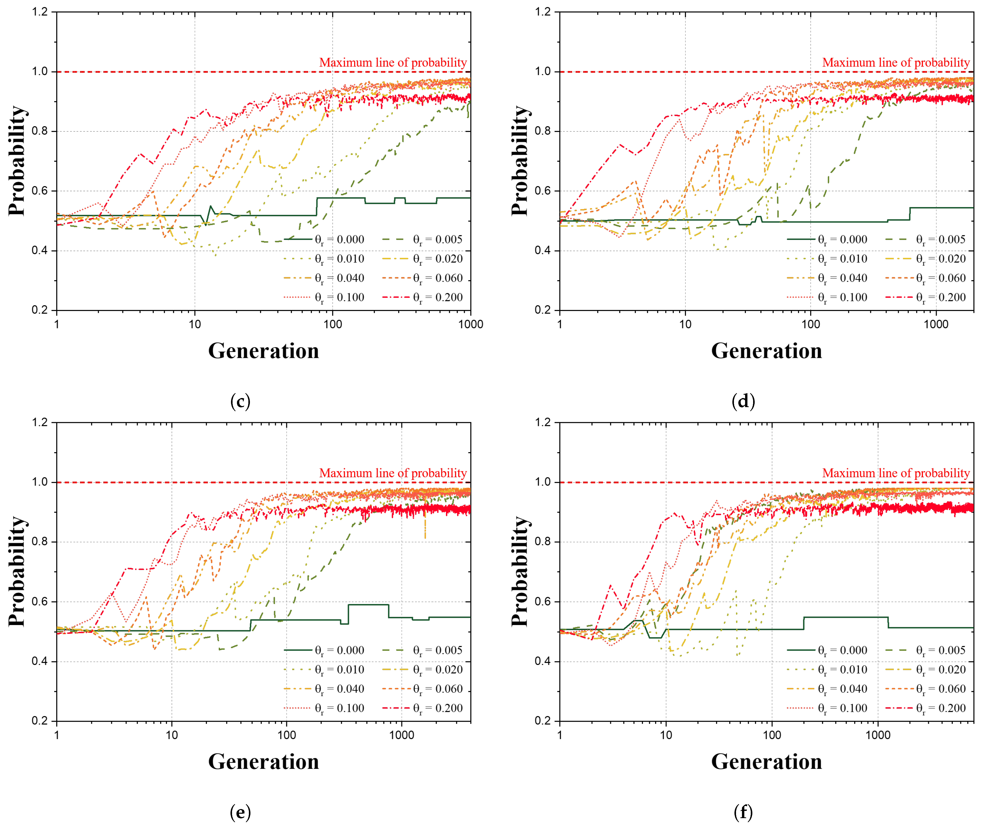
Figure 5 is the qubit probability according to the number of generations. Regardless of the size of $ϵ$, as the number of generations progresses, the qubit converges to one value. However, as $ϵ$ increases, it converges at a value far from 1.0. Therefore, it was confirmed that an appropriate $ϵ$ exists to increase convergence performance, and in this paper, the convergence performance was the best when the range was 0.005–0.015.

3.4. ${\theta }_r$

${\theta }_r$ is a parameter used in the rotation gate, and the rotation angle of the qubit is determined by the size of ${\theta }_r$. It can be predicted that if ${\theta }_r$ has a large value, the qubit will converge quickly, and if ${\theta }_r$ has a small value, the qubit will converge slowly. ${\theta }_r$ was changed to 0.00, 0.05, 0.01, 0.02, 0.04, 0.06, 0.1, and 0.2, and other parameters were used as well, as shown in

Table 6. Parameters for ${\theta }_r$ analysis.

d	QHMS	QHMCR	QPAR	$\mathit{ϵ}$	${\mathit{\theta }}_{\mathit{r}}$	Mea.	$\mathit{qbw}$
							tolBW	${\mathit{qbw}}_{\mathit{max}}$	${\mathit{qbw}}_{\mathit{min}}$
20	10	0.9	0.1	0.01	0.00–0.2	1	0.95	1.0	0.01

. The interpretation was repeated 50 times.

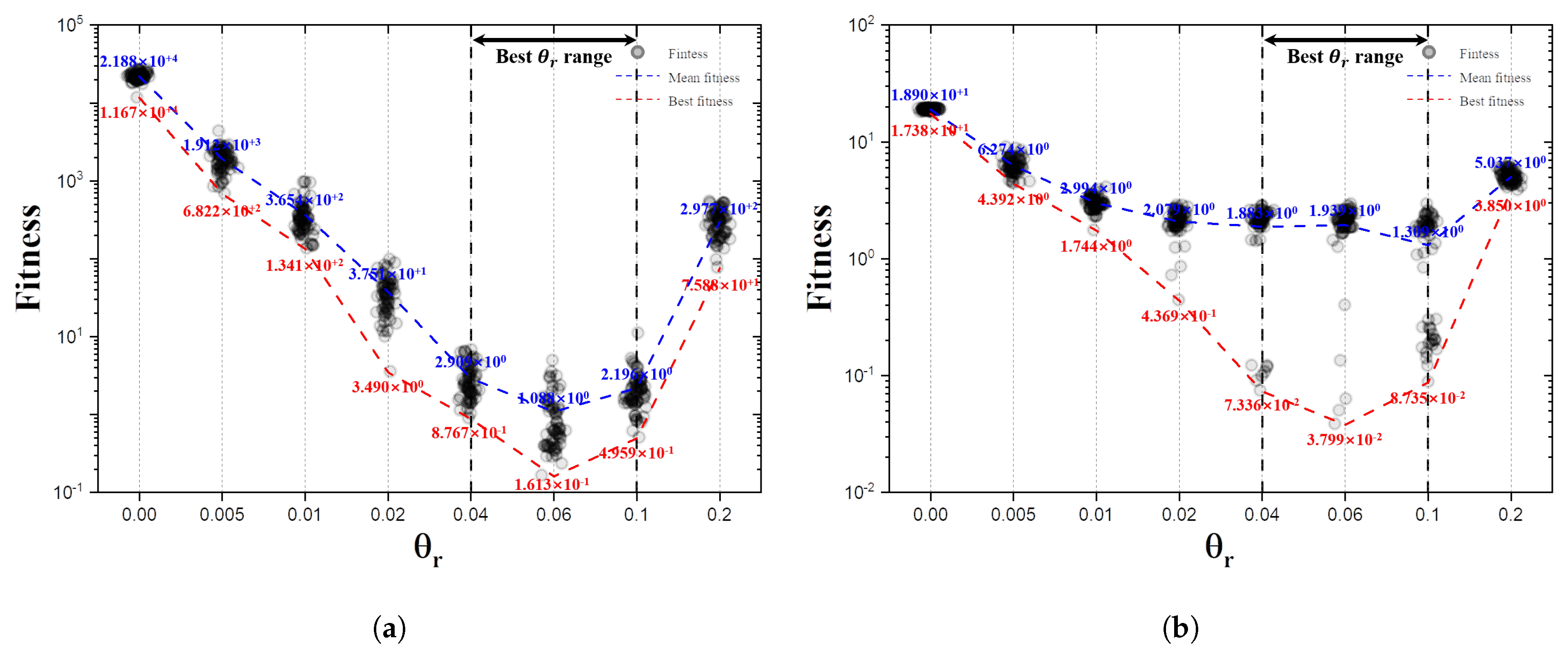
Figure 6 presents the change in the best or mean fitness according to the change in ${\theta }_r$, and the analysis results are summarized in

Table A4. Benchmark function results according to ${\theta }_r$.

Funct.	Index	${\mathit{\theta }}_{\mathit{r}}$
		0.000	0.005	0.010	0.020	0.040	0.060	0.100	0.200
$f_{01}$	BF	1.167 $\times {10}^{+4}$	6.822 $\times {10}^{+2}$	1.341 $\times {10}^{+2}$	3.490 $\times {10}^0$	8.767 $\times {10}^{-1}$	1.613 $\times {10}^{-1}$	4.959 $\times {10}^{-1}$	7.588 $\times {10}^{+1}$
	MF	2.188 $\times {10}^{+4}$	1.912 $\times {10}^{+3}$	3.654 $\times {10}^{+2}$	3.751 $\times {10}^{+1}$	2.909 $\times {10}^0$	1.088 $\times {10}^0$	2.196 $\times {10}^0$	2.977 $\times {10}^{+2}$
	Std	2.723 $\times {10}^{+3}$	6.883 $\times {10}^{+2}$	1.985 $\times {10}^{+2}$	2.118 $\times {10}^{+1}$	1.545 $\times {10}^0$	9.910 $\times {10}^{-1}$	1.631 $\times {10}^0$	1.196 $\times {10}^{+2}$
$f_{02}$	BF	1.738 $\times {10}^{+1}$	4.392 $\times {10}^0$	1.744 $\times {10}^0$	4.369 $\times {10}^{-1}$	7.336 $\times {10}^{-2}$	3.799 $\times {10}^{-2}$	8.735 $\times {10}^{-2}$	3.850 $\times {10}^0$
	MF	1.890 $\times {10}^{+1}$	6.274 $\times {10}^0$	2.994 $\times {10}^0$	2.079 $\times {10}^0$	1.883 $\times {10}^0$	1.939 $\times {10}^0$	1.309 $\times {10}^0$	5.037 $\times {10}^0$
	Std	3.998 $\times {10}^{-1}$	1.069 $\times {10}^0$	4.198 $\times {10}^{-1}$	5.096 $\times {10}^{-1}$	7.852 $\times {10}^{-1}$	6.986 $\times {10}^{-1}$	8.848 $\times {10}^{-1}$	6.141 $\times {10}^{-1}$
$f_{03}$	BF	1.144 $\times {10}^{+2}$	1.387 $\times {10}^0$	8.973 $\times {10}^{-1}$	1.770 $\times {10}^{-1}$	3.009 $\times {10}^{-3}$	1.972 $\times {10}^{-3}$	9.346 $\times {10}^{-2}$	1.238 $\times {10}^0$
	MF	1.738 $\times {10}^{+2}$	2.242 $\times {10}^0$	1.083 $\times {10}^0$	4.677 $\times {10}^{-1}$	1.530 $\times {10}^{-1}$	1.338 $\times {10}^{-1}$	3.247 $\times {10}^{-1}$	2.196 $\times {10}^0$
	Std	2.184 $\times {10}^{+1}$	4.968 $\times {10}^{-1}$	5.778 $\times {10}^{-2}$	1.670 $\times {10}^{-1}$	1.127 $\times {10}^{-1}$	1.122 $\times {10}^{-1}$	1.638 $\times {10}^{-1}$	5.735 $\times {10}^{-1}$
$f_{04}$	BF	1.536 $\times {10}^{+2}$	1.249 $\times {10}^{+1}$	1.146 $\times {10}^{+1}$	1.218 $\times {10}^{+1}$	1.167 $\times {10}^{+1}$	1.068 $\times {10}^{+1}$	1.319 $\times {10}^{+1}$	2.416 $\times {10}^{+1}$
	MF	1.860 $\times {10}^{+2}$	2.738 $\times {10}^{+1}$	2.569 $\times {10}^{+1}$	2.239 $\times {10}^{+1}$	2.419 $\times {10}^{+1}$	2.279 $\times {10}^{+1}$	2.324 $\times {10}^{+1}$	4.346 $\times {10}^{+1}$
	Std	1.141 $\times {10}^{+1}$	7.019 $\times {10}^0$	8.376 $\times {10}^0$	6.382 $\times {10}^0$	6.914 $\times {10}^0$	6.321 $\times {10}^0$	6.296 $\times {10}^0$	8.413 $\times {10}^0$
$f_{05}$	BF	3.581 $\times {10}^{+3}$	1.999 $\times {10}^{+2}$	1.303 $\times {10}^{+2}$	1.378 $\times {10}^{+2}$	1.035 $\times {10}^{+2}$	1.577 $\times {10}^{+2}$	1.536 $\times {10}^{+2}$	3.001 $\times {10}^{+2}$
	MF	4.287 $\times {10}^{+3}$	5.863 $\times {10}^{+2}$	5.391 $\times {10}^{+2}$	5.645 $\times {10}^{+2}$	4.983 $\times {10}^{+2}$	5.890 $\times {10}^{+2}$	4.393 $\times {10}^{+2}$	7.602 $\times {10}^{+2}$
	Std	2.986 $\times {10}^{+2}$	2.028 $\times {10}^{+2}$	1.849 $\times {10}^{+2}$	2.168 $\times {10}^{+2}$	2.387 $\times {10}^{+2}$	2.041 $\times {10}^{+2}$	1.775 $\times {10}^{+2}$	2.223 $\times {10}^{+2}$
$f_{06}$	BF	6.081 $\times {10}^{+6}$	1.714 $\times {10}^{+1}$	1.729 $\times {10}^{+1}$	1.767 $\times {10}^{+1}$	1.584 $\times {10}^{+1}$	1.809 $\times {10}^{+1}$	1.716 $\times {10}^{+1}$	4.437 $\times {10}^{+1}$
	MF	1.844 $\times {10}^{+7}$	2.872 $\times {10}^{+2}$	2.439 $\times {10}^{+2}$	2.139 $\times {10}^{+2}$	2.914 $\times {10}^{+2}$	2.171 $\times {10}^{+2}$	2.286 $\times {10}^{+2}$	4.657 $\times {10}^{+2}$
	Std	5.343 $\times {10}^{+6}$	5.463 $\times {10}^{+2}$	4.703 $\times {10}^{+2}$	3.005 $\times {10}^{+2}$	5.546 $\times {10}^{+2}$	4.317 $\times {10}^{+2}$	4.018 $\times {10}^{+2}$	6.146 $\times {10}^{+2}$
Ranking	BF	8.00	4.67	3.67	4.00	2.67	3.50	3.83	5.67
	MF	8.00	6.17	4.67	3.00	3.17	2.50	2.17	6.33
	AVG(BF, MF)	8.00	5.42	4.17	3.50	2.92	3.00	3.00	6.00

. Checking for the best fitness, $f_{01}$, $f_{02}$, $f_{03}$, and $f_{04}$ were closest to Min when ${\theta }_r$ was 0.060, and $f_{05}$ and $f_{06}$ were closest when ${\theta }_r$ was 0.040. In addition, when ${\theta }_r$ was 0.000, the convergence performance was the worst for all functions because there was no rotation angle of the qubit. Checking the average values using BF and MF in Table A4, it can be seen that the convergence performance is the best when ${\theta }_r$ has a range of 0.040–0.100.

Figure 7 is the qubit probability according to the number of generations. All functions converge to one value as the number of generations progresses, except when ${\theta }_r$ is 0.000. In particular, the larger ${\theta }_r$ is, the faster it converges to one value. However, when ${\theta }_r$ is 0.2, the angle of rotation is so large that it converges near 0.9 and not any further.

Therefore, it is confirmed that ${\theta }_r$ of an appropriate size exists to improve the convergence performance of the QbHS algorithm. In this paper, the convergence performance was the best when ${\theta }_r$ was in the range 0.040–0.100.

4. Truss Structure Example

The weight optimization of truss structures is aimed at the minimum weight of the problem structure and can be defined as Equation (13). Equation (14) is a constraint for performing weight optimization [42].

$$\begin{array}{cc}\hfill \mathrm{Minimize}& F\left(x\right)=\left(\rho \sum _{i=1}^n{B}_i{A}_i{L}_i+\sum _{j=1}^m{b}_j\right)\ast penalty\hfill \end{array}$$

(13)

$$\begin{array}{cc}\hfill \mathrm{Subject}\mathrm{to}& g_k\left(x\right)\le 0,k=1,2,3,4,5,6,7\hfill \\ \hfill & \\ \hfill & g_1\left(x\right)=\left|B_i{\sigma }_i\right|-{\sigma }_i^{max}\le 0\hfill \\ \hfill & g_2\left(x\right)=\left|{\delta }_j\right|-{\delta }_j^{max}\le 0\hfill \\ \hfill & g_3\left(x\right)=\left|B_i{\sigma }_i^{comp}\right|-{\sigma }_i^{cr}\le 0,{\sigma }_i^{cr}=\frac{k_i{A}_i{E}_i}{L_i^2}\hfill \\ \hfill & g_4\left(x\right)=f_r-r_r^{max}\le 0\hfill \\ \hfill & g_5\left(x\right)=A_{min}\le A_i\le A_{max}\hfill \\ \hfill & g_6=Checkvalidityofstructure\hfill \\ \hfill & g_7=Checkkinematicstability\hfill \end{array}$$

(14)

The cross-section that each truss structure element may have is discrete.

Table A5. Discrete area of truss structure.

No.	Area (cm${}^2$)	Thickness (cm)	No.	Area (cm${}^2$)	Thickness (cm)
1	0.7161	0.1510	33	24.7741	0.8880
2	0.9097	0.1702	34	24.9677	0.8915
3	1.2645	0.2006	35	25.0322	0.8926
4	1.6129	0.2266	36	26.9677	0.9265
5	1.9806	0.2511	37	27.2258	0.9309
6	2.5226	0.2834	38	28.9677	0.9602
7	2.8516	0.3013	39	29.6128	0.9709
8	3.6323	0.3400	40	30.9677	0.9928
9	3.8839	0.3516	41	32.0645	1.0103
10	4.9419	0.3966	42	33.0322	1.0254
11	5.0645	0.4015	43	37.0322	1.0857
12	6.4129	0.4518	44	46.5806	1.2177
13	6.4516	0.4532	45	51.4193	1.2793
14	7.9226	0.5022	46	51.4193	1.2793
15	8.1677	0.5099	47	59.9999	1.3820
16	9.4000	0.5470	48	69.9999	1.4927
17	10.0839	0.5666	49	74.1943	1.5368
18	10.4516	0.5768	50	87.0966	1.6650
19	11.6129	0.6080	51	89.6772	1.6895
20	12.8387	0.6393	52	91.6127	1.7077
21	13.7419	0.6614	53	99.9998	1.7841
22	15.3548	0.6991	54	103.2256	1.8127
23	16.9032	0.7335	55	109.0320	1.8630
24	16.9677	0.7349	56	121.2901	1.9649
25	18.5806	0.7691	57	128.3868	2.0216
26	18.9032	0.7757	58	141.9352	2.1255
27	19.9354	0.7966	59	147.7416	2.1686
28	20.1935	0.8017	60	158.0642	2.2431
29	21.8064	0.8331	61	170.9674	2.3328
30	22.3871	0.8442	62	180.6448	2.3979
31	22.9032	0.8538	63	193.5480	2.4821
32	23.4193	0.8634	64	216.1286	2.6229

is the size of the cross-sectional area that each member can have and may have a total of 64 cross-sectional areas [43]. A total of 7 constraints were used for weight optimization of the truss structure. $g_1$, $g_2$, $g_3$, and $g_4$ utilize the maximum stress of the member, the maximum displacement of the node, the buckling stress, and the natural frequency of the structure through FEA (finite element analysis) of the structure. A penalty of ${10}^4$ is given if the constraint is not satisfied. $g_5$ is the range of cross-sectional areas that the element can have. $g_6$ evaluates the validity of the structure. That is, it determines whether there is a node serving as a support and a node acting as a load. A penalty of ${10}^9$ is given if the constraint is not satisfied. $g_7$ evaluates the kinetic stability of the structure. To evaluate kinetic stability, check the degree of freedom and stiffness matrix of the structure. If the degree of freedom of the structure is greater than 0, a penalty of ${10}^8$ is given. In addition, if eig(K) is less than ${10}^{-5}$, a penalty of ${10}^7$ is given.

The QEA algorithm was used to compare the weight optimization results of the QbHS algorithm.

Table 7. Parameter for weight optimization of truss structures.

Algorithm	Parameters
QbHSA	$QHMS$ = 10, $QHMCR$ = 0.9, $QPAR$ = 0.1, $qubit$ = 18, $ϵ$ = 0.01, ${\theta }_r$ = 0.06, $Mea.$ = 2, $tolBW$ = 0.95, $BWQ$ = 0.3, $qb{w}_{max}$ = 1.0, $qb{w}_{min}$ = 0.01
QEA	Local group size = 10, Global migration period = 100, $qubit$ = 18, $ϵ$ = 0.01, ${\theta }_r$ = 0.06, $Mea.$ = 2

presents parameters used in the QbHS and QEA algorithms to perform weight optimization, which was repeatedly interpreted 100 times.

4.1. 20-Bar Truss Structure

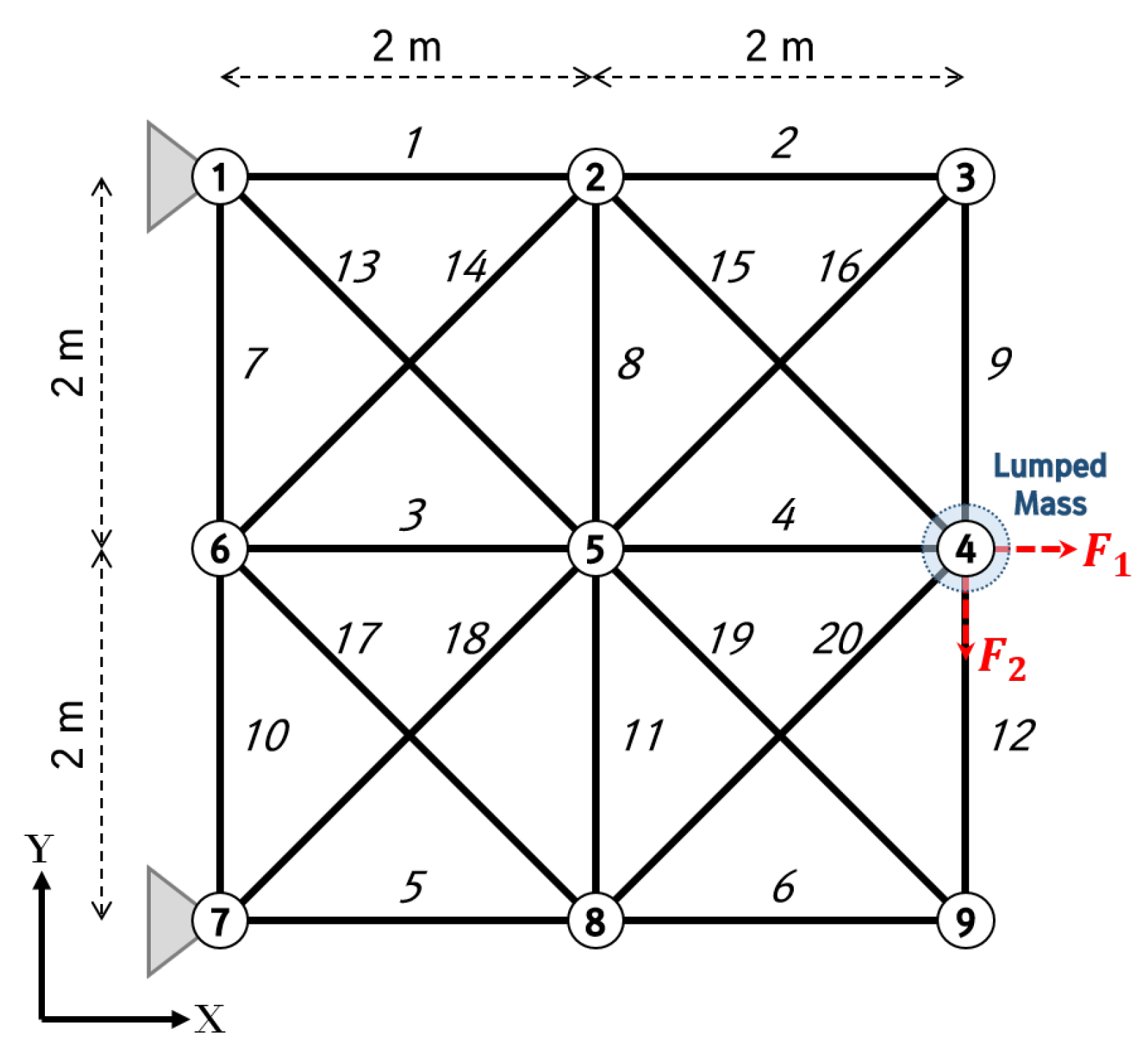
Figure 8 is the initial shape of a 20-bar truss structure, consisting of 9 nodes and 20 elements. E and $\rho$ are 200,000 MPa and 7860 kg/m${}^3$, respectively, and the loading conditions are classified into two cases. The first case is $F_1$ = 500 kN and $F_2$ = 0 kN, and the second case is $F_1$ = 0 kN and $F_2$ = 500 kN. The allowable stress of each element is 180 MPa, and the maximum displacement that can occur on the Y-axis of the 4-node is 10 mm. Finally, the first natural frequency should be more than 60 Hz, and the second natural frequency should be more than 100 Hz.

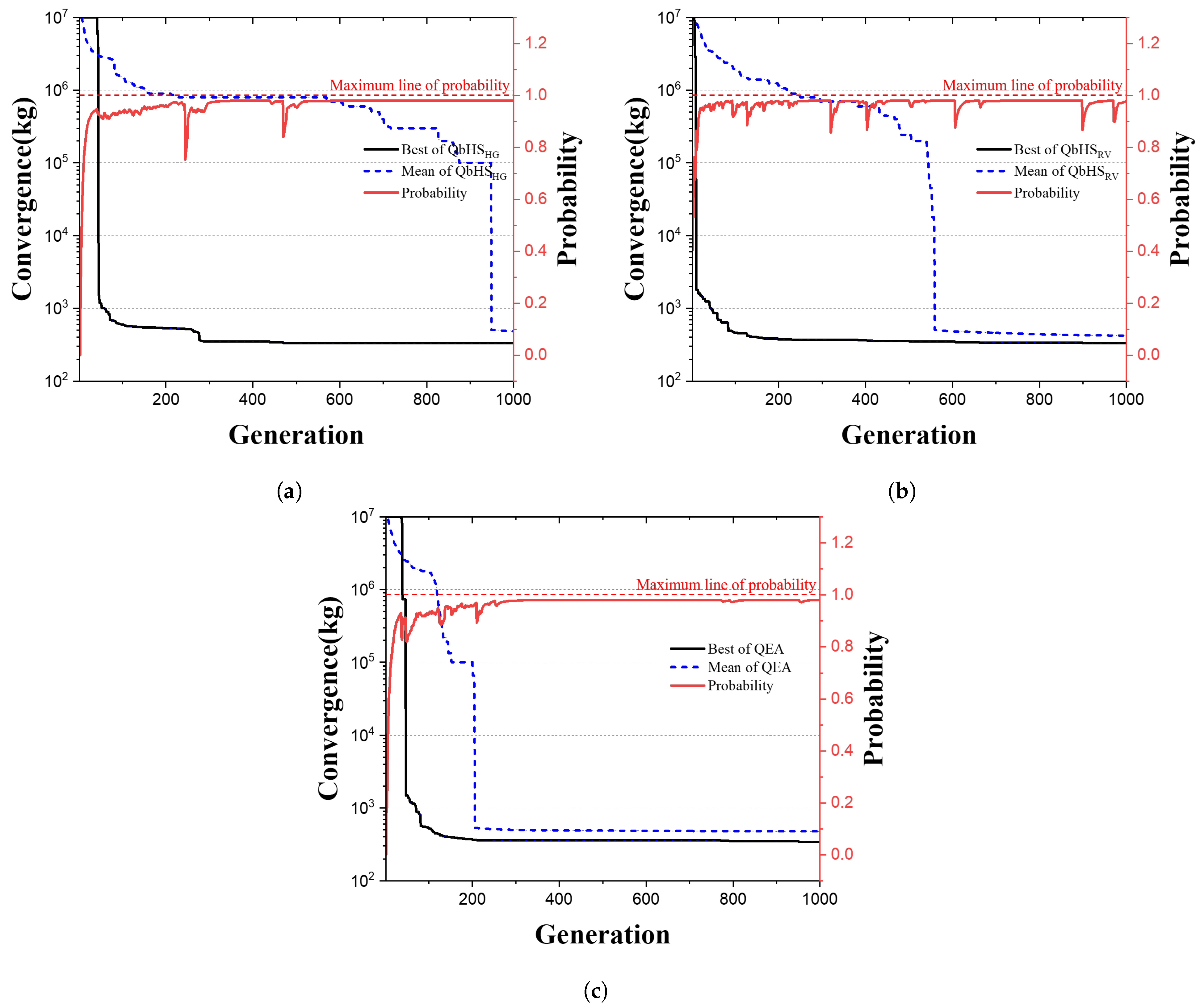
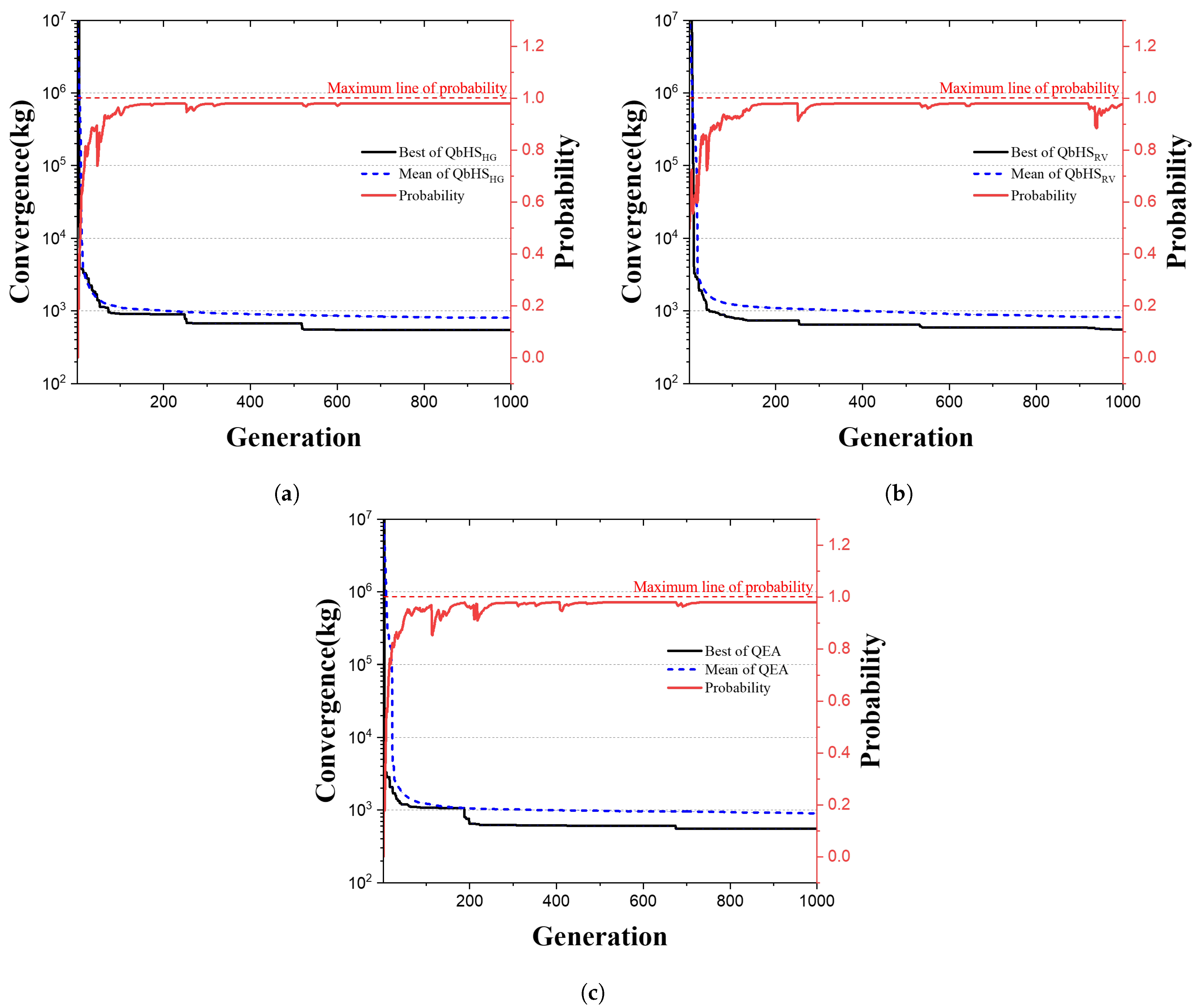
Figure 9 is a convergence result graph for a 20-bar truss structure. For all three sets of algorithm results, the best and mean weights converge to one value. The best weights were derived as 332.503 kg for the QbHS${}_{HG}$ algorithm, 331.211 kg for the QbHS${}_{RV}$ algorithm, and 344.095 kg for the QEA algorithm. The mean weights were derived as 485.021 kg for the QbHS${}_{HG}$ algorithm, 422.130 kg for the QbHS${}_{RV}$ algorithm, and 478.228 kg for the QEA algorithm. The qubit probability shows that all algorithms converge to values close to 1.

Table 8. Results of the 20-bar truss structure.

Variable	QbHS${}_{\mathit{HG}}$	QbHS${}_{\mathit{RV}}$	QE
$A_1$	26	23	20
$A_2$	-	-	-
$A_3$	-	-	-
$A_4$	-	-	21
$A_5$	24	25	32
$A_6$	-	-	-
$A_7$	-	-	-
$A_8$	24	33	21
$A_9$	-	-	-
$A_{10}$	-	-	-
$A_{11}$	24	25	22
$A_{12}$	-	-	-
$A_{13}$	27	27	32
$A_{14}$	-	-	-
$A_{15}$	27	27	25
$A_{16}$	-	-	-
$A_{17}$	-	-	-
$A_{18}$	32	27	25
$A_{19}$	-	-	-
$A_{20}$	32	27	33
Best (kg)	332.503	331.211	344.095
Mean (kg)	485.021	422.130	478.228
Std	92.247	61.786	103.993
${\sigma }_{max}$ (MPa)	177.35	177.35	179.61
${\sigma }_{max}^{cr}$ (MPa)	339.35	495.48	468.39
${\delta }_{4y}^{max}$ (mm)	9.438	9.684	9.829
f${}_1$ (Hz)	80.202	79.226	78.543
f${}_2$ (Hz)	100.004	100.141	134.305

presents the weight optimization results of the 20-bar truss structure. Three algorithms contain elements 1, 5, 8, 11, 13, 15, 18, and 20, and the QbHS${}_{RV}$ algorithm adds element 4. Therefore, the QbHS${}_{HG}$ and QbHS${}_{RV}$ algorithms adopted a total of eight elements, and the QEA algorithm adopted a total of nine elements. Among the results of the three algorithms, the QbHS${}_{RV}$ algorithm had the best convergence performance by deriving the best, mean, and standard deviation (Std) of 331.211 kg, 422.130 kg, and 61.786, respectively.

4.2. 24-Bar Truss Structure

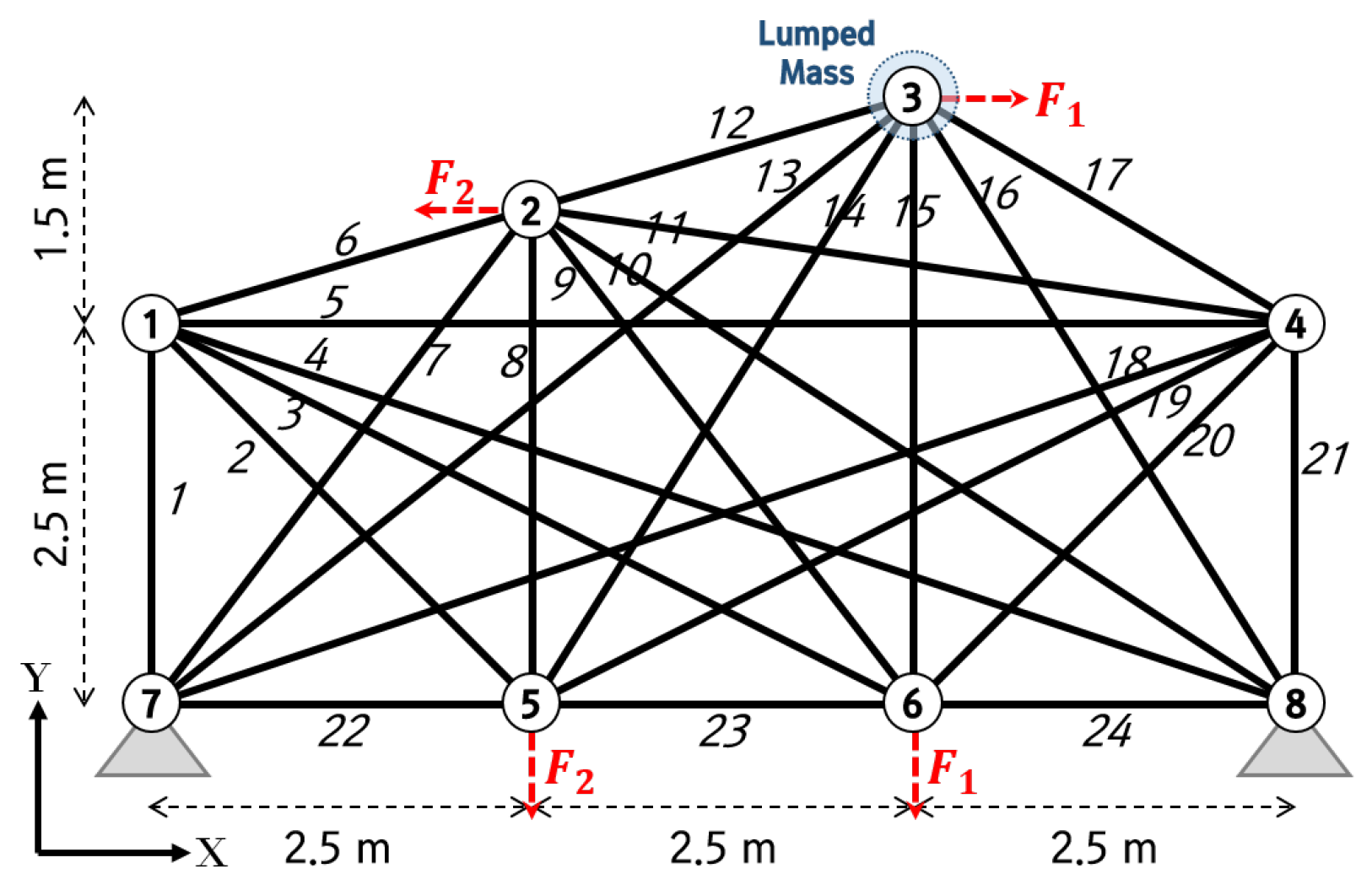
Figure 10 is the initial shape of the 24-bar truss structure, consisting of 8 nodes and 24 elements. E and $\rho$ are 200,000 MPa and 7860 kg/m${}^3$, respectively, and the loading conditions are classified into two cases. The first case is $F_1$ = 100 kN and $F_2$ = 0 kN, and the second case is $F_1$ = 0 kN and $F_2$ = 100 kN. The allowable stress of each element is 180 MPa, and the maximum displacement that can occur on the Y-axis of the 5, 6-node is 10 mm. Finally, the first natural frequency should be more than 30 Hz.

Figure 11 is a convergence result graph of a 24-bar truss structure. In all three algorithm results, the best and mean weights converge to one value. The best weights were 243.762 kg for the QbHS${}_{HG}$ algorithm, 250.718 kg for the QbHS${}_{RV}$ algorithm, and 264.944 kg for the QEA algorithm. The mean weights were derived as 364.978 kg for the QbHS${}_{HG}$ algorithm, 342.582 kg for the QbHS${}_{RV}$ algorithm, and 364.060 kg for the QEA algorithm. The qubit probability shows that all algorithms converge to values close to 1.

Table 9. Results of the 24-bar truss structure.

Variable	QbHS${}_{\mathit{HG}}$	QbHS${}_{\mathit{RV}}$	QE
$A_1$	-	-	-
$A_2$	-	-	-
$A_3$	-	-	-
$A_4$	-	-	-
$A_5$	-	-	-
$A_6$	-	-	-
$A_7$	25	32	32
$A_8$	12	12	12
$A_9$	12	1	16
$A_{10}$	-	-	-
$A_{11}$	-	-	-
$A_{12}$	8	4	9
$A_{13}$	-	-	-
$A_{14}$	-	9	1
$A_{15}$	9	12	12
$A_{16}$	-	27	28
$A_{17}$	17	-	-
$A_{18}$	-	-	-
$A_{19}$	-	-	-
$A_{20}$	17	-	-
$A_{21}$	17	-	-
$A_{22}$	1	9	-
$A_{23}$	-	8	-
$A_{24}$	17	-	8
Best (kg)	243.762	250.718	264.944
Mean (kg)	364.978	342.582	364.060
Std	91.223	72.289	73.645
${\sigma }_{max}$ (MPa)	155.94	162.50	175.43
${\sigma }_{max}^{cr}$ (MPa)	129.07	111.44	111.44
${\delta }_{5y}^{max}$ (mm)	3.267	1.657	3.048
${\delta }_{6y}^{max}$ (mm)	3.03	9.684	9.829
f${}_1$ (Hz)	32.024	30.549	33.925

presents the weight optimization results of the 24-bar truss structure. As a result of weight optimization, all three algorithms contain elements 7, 8, 9, 12, and 15, and the QbHS${}_{HG}$ algorithm adds elements 17, 20, 21, and 22. The QbHS${}_{RV}$ algorithm adds elements 14, 16, 22, and 23, and the QEA algorithm adds elements 14, 16, and 24. Thus, the QbHS${}_{HG}$ algorithm adopted a total of 10 elements, the QbHS${}_{RV}$ algorithm a total of 9 elements, and the QEA algorithms a total of 8 elements. The QbHS${}_{RV}$ algorithm derived 243.762 kg from the best weight, which was the best convergence performance, but the results of the QbHS${}_{RV}$ algorithm, 342.582 kg and 72.289 for the mean and std, were the best. In addition, the results of the three algorithms satisfied all constraints.

4.3. 72-Bar Truss Structure

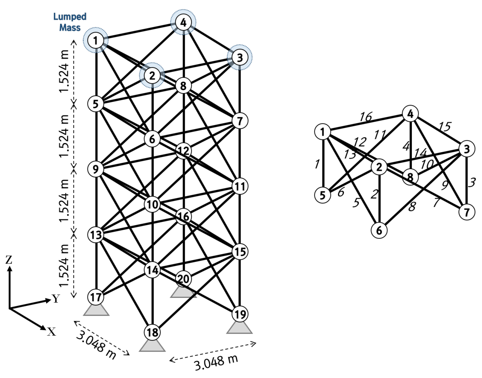
Figure 12 is the initial shape of a 72-bar truss structure, consisting of 20 nodes and 72 elements. The 72 elements were grouped into a total of 16 ($G_1$–$G_{16}$) and are shown in Table A5. E and $\rho$ are 68,950 MPa and 2767.99 kg/m${}^3$, respectively. The loading conditions are also classified into two cases. The first case has a load of 22.25 kN applied in the X, Y, and −Z directions at node 1. In the second case, 22.25 kN is applied in the −Z direction of nodes 1, 2, 3, and 4. The allowable stress of each element is 172.375 MPa, and the maximum displacement that can occur on the X or Y axis of nodes 1, 2, 3, and 4 is 6.35 mm. Finally, the first natural frequency should be more than 4 Hz, and the third natural frequency should be more than 6 Hz.

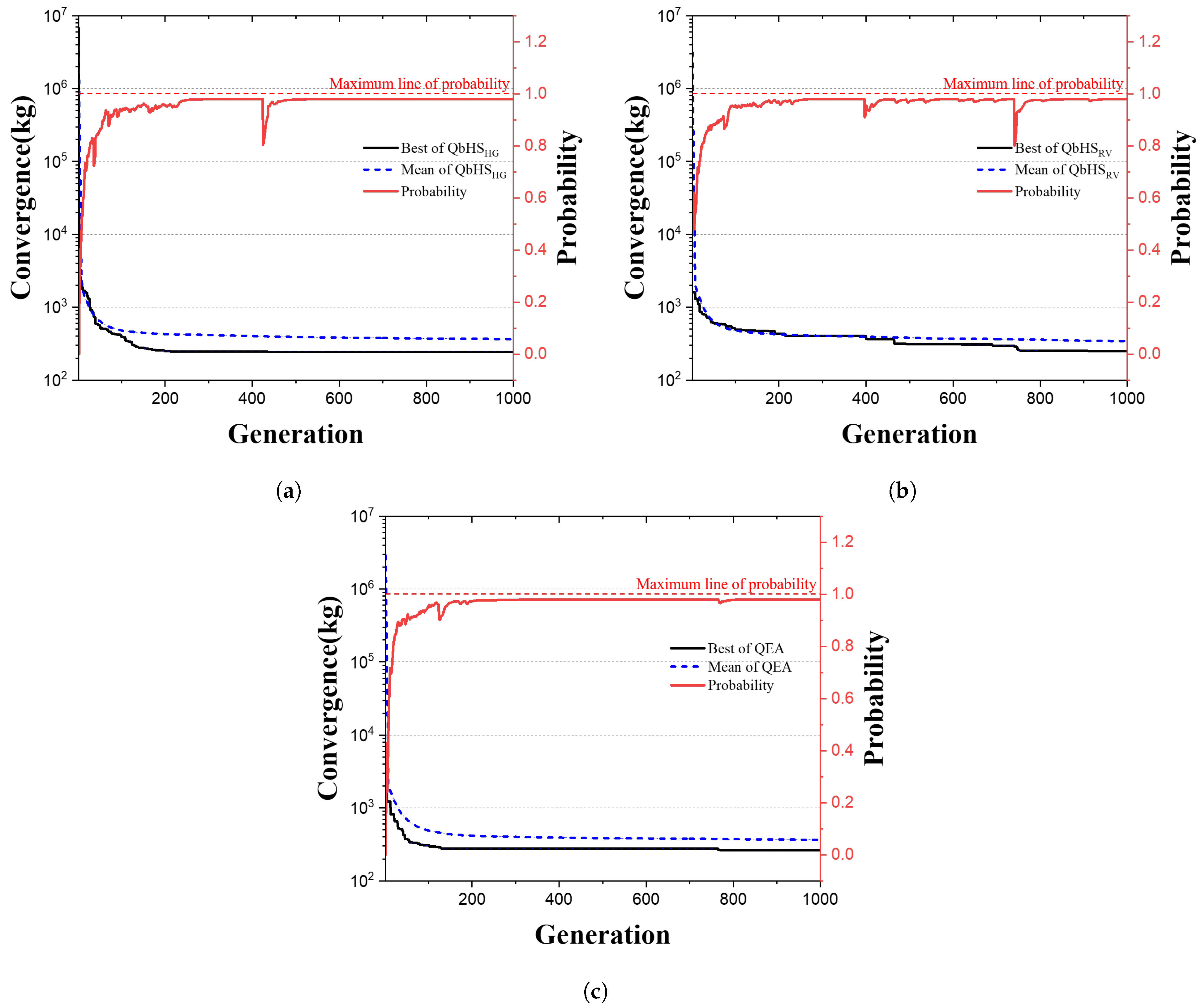
Figure 13 is a convergence result graph of a 72-bar truss structure. The results of the three algorithms show that the best and mean weight converge to one value. The weight optimization of the 72-bar truss structure resulted in the best weights of 445.833 kg for the QbHS${}_{HG}$ algorithm, 449.190 kg for the QbHS${}_{RV}$ algorithm, and 446.018 kg for the QEA algorithm. Mean weights were derived as 484.945 kg for the QbHS${}_{HG}$ algorithm, 498.136 kg for the QbHS${}_{RV}$ algorithm, and 522.369 kg for the QEA algorithm. The qubit probability shows that all algorithms converge to values close to 1.

Table 10. Results of the 72-bar truss structure.

Variable	QbHS${}_{\mathit{HG}}$	QbHS${}_{\mathit{RV}}$	QE
$G_1$	6	8	6
$G_2$	8	8	8
$G_3$	9	8	8
$G_4$	10	10	10
$G_5$	9	8	8
$G_6$	8	8	9
$G_7$	-	-	-
$G_8$	-	-	-
$G_9$	9	9	9
$G_{10}$	8	8	8
$G_{11}$	-	-	-
$G_{12}$	-	-	-
$G_{13}$	9	9	9
$G_{14}$	8	8	8
$G_{15}$	-	-	-
$G_{16}$	-	-	-
Best (kg)	549.954	551.654	551.729
Mean (kg)	806.250	816.971	900.185
Std	177.718	238.728	260.150
${\sigma }_{max}$ (MPa)	86.59	81.91	86.78
${\sigma }_{max}^{cr}$ (MPa)	133.78	133.78	133.78
${\delta }^{max}$ (mm)	2.942	2.968	2.932
f${}_1$ (Hz)	4.008	4.013	4.008
f${}_3$ (Hz)	6.883	6.883	6.940

presents the weight optimization results of the 72-bar truss structure. The results of all three algorithms include groups 1, 2, 5, 6, 9, 10, 13, and 14, and the QbHS${}_{HG}$ algorithm adds groups 8 and 11. The QbHS${}_{RV}$ algorithm adds groups 4 and 15, and the QEA algorithm adds groups 8 and 15. Therefore, all three algorithms adopted a total of 10 groups. The best, mean, and std of the QbHS${}_{RV}$ algorithm were 445.833 kg, 484.945 kg, and 21.306, respectively, showing the best convergence performance. In addition, the results of the three algorithms satisfied all constraints.

5. Conclusions

In this paper, the convergence performance of the QbHS algorithm, which combines quantum computing and conventional HS algorithms, was compared according to parameter changes. In addition, the weight optimization of 20-bar, 24-bar, and 72-bar truss structures with discrete cross-sectional areas was performed.

• First, the convergence performance according to the size change of each parameter was compared. The convergence performance of the QbHS algorithm was better because the QHM increased as the QHMS increased. The larger the value of QHMCR, and the smaller the value of QPAR, the better the convergence performance of the QbHS algorithm. This aspect is judged to be similar to the conventional HS algorithm. The convergence performance of the QbHS algorithm was the best when $ϵ$ had a range of 0.005–0.015 and ${\theta }_r$ had a range of 0.040–0.100.
• The weight optimization of 20-bar, 24-bar, and 72-bar truss structures with discrete cross-sectional areas was performed using the QbHS algorithm. For the 20-bar truss structure, the QbHS${}_{RV}$ algorithm derived it as 331.211 kg, and for the 24-bar truss structure, the QbHS${}_{HG}$ algorithm derived it as 243.762 kg. The 72-bar truss structure was derived as 549.954 kg by the QbHS${}_{HG}$ algorithm.

Therefore, the convergence performance according to the changes in the parameters of the QbHS algorithm was compared using the six benchmark functions, and a parameter that could derive the best convergence performance was proposed. In addition, by applying it to the weight optimization of truss structures with discrete cross-sectional areas, a lower weight was derived than the QE algorithm, confirming that the convergence performance was better.

Research that combines quantum computing with existing metaheuristic algorithms, such as the QbHS algorithm, is creating new fields. However, it is extremely rare to apply quantum computing-based metaheuristics algorithms to engineering problems. Thus, quantum computing-based metaheuristic algorithms require a considerable amount of effort to solve optimization problems in engineering fields such as structures, machinery, and mechatronics. In addition, the truss structure applied in this paper is a basic structure, but it needs to be applied to optimize various structures such as large trusses and dome structures or complex buildings. Finally, since quantum computing-based metaheuristic algorithms are still in an early stage, it is necessary to combine them with various metaheuristic algorithms and develop various quantum operators. The application of various engineering problems of quantum computing-based metaheuristic algorithms and the development of quantum operators are expected to expand the field of computer information.

References

1. Morsch, O. Quantum Bits and Quantum Secrets: How Quantum Physics Is Revolutionizing Codes and Computers; John Wiley & Sons: Hoboken, NJ, USA, 2008. [Google Scholar]
2. Jones, J.A. Quantum computing with NMR. arXiv 2010, arXiv:1011.1382. [Google Scholar]
3. Berthiaume, A.; Feynman, R.P. Quantum computation. Complex. Theory Retrosp. II 1997, 2, 23. [Google Scholar]
4. Shor, P.W. Algorithms for quantum computation: Discrete logarithms and factoring. In Proceedings of the 35th Annual Symposium on Foundations of Computer Science, Santa Fe, NM, USA, 20–22 November 1994; pp. 124–134. [Google Scholar]
5. Monz, T.; Nigg, D.; Martinez, E.A.; Brandl, M.F.; Schindler, P.; Rines, R.; Wang, S.X.; Chuang, I.L.; Blatt, R. Realization of a scalable Shor algorithm. Science 2016, 351, 1068–1070. [Google Scholar] [CrossRef]
6. Bernstein, D.J. Grover vs. mceliece. In Proceedings of the Post-Quantum Cryptography: 3rd International Workshop, PQCrypto, Darmstadt, Germany, 25–28 May 2010; pp. 73–80. [Google Scholar]
7. National Academies of Sciences, Engineering, and Medicine and others. Quantum Computing: Progress and Prospects; The National Academies Press: Washington, DC, USA, 2019. [Google Scholar]
8. Zhang, J.; Tian, Q.; Tang, C.; Wang, L.; Xu, J.; Fang, J. Study on Worldwide Development and Trends of Quantum Technologies Based on Patent Data. Int. J. Inf. Educ. Technol. 2020, 10, 239–244. [Google Scholar] [CrossRef]
9. Ross, O.H.M. A review of quantum-inspired metaheuristics: Going from classical computers to real quantum computers. IEEE Access 2019, 8, 814–838. [Google Scholar] [CrossRef]
10. Gharehchopogh, F.S. Quantum-inspired metaheuristic algorithms: Comprehensive survey and classification. Artif. Intell. Rev. 2023, 56, 5479–5543. [Google Scholar] [CrossRef]
11. Xiao, F.; Hulsey, J.L.; Chen, G.S.; Xiang, Y. Optimal static strain sensor placement for truss bridges. Int. J. Distrib. Sens. Netw. 2017, 13, 1550147717707929. [Google Scholar] [CrossRef]
12. Xiao, F.; Zhu, W.; Meng, X.; Chen, G.S. Parameter identification of structures with different connections using static responses. Appl. Sci. 2022, 12, 5896. [Google Scholar] [CrossRef]
13. Xiao, F.; Sun, H.; Mao, Y.; Chen, G.S. Damage identification of large-scale space truss structures based on stiffness separation method. In Structures; Elsevier: Amsterdam, The Netherlands, 2023; Volume 53, pp. 109–118. [Google Scholar]
14. Rayegani, A.; Nouri, G. Seismic collapse probability and life cycle cost assessment of isolated structures subjected to pounding with smart hybrid isolation system using a modified fuzzy based controller. In Structures; Elsevier: Amsterdam, The Netherlands, 2022; Volume 44, pp. 30–41. [Google Scholar]
15. Rayegani, A.; Nouri, G. Application of smart dampers for prevention of seismic pounding in isolated structures subjected to near-fault earthquakes. J. Earthq. Eng. 2022, 26, 4069–4084. [Google Scholar] [CrossRef]
16. Narayanan, A.; Moore, M. Quantum-inspired genetic algorithms. In Proceedings of the IEEE International Conference on Evolutionary Computation, Nagoya, Japan, 20–22 May 1996; pp. 61–66. [Google Scholar]
17. Han, K.H.; Kim, J.H. Genetic quantum algorithm and its application to combinatorial optimization problem. In Proceedings of the Congress on Evolutionary Computation, CEC00 (Cat. No. 00TH8512), La Jolla, CA, USA, 16–19 July 2000; Volume 2, pp. 1354–1360. [Google Scholar]
18. Han, K.H.; Kim, J.H. Quantum-inspired evolutionary algorithm for a class of combinatorial optimization. IEEE Trans. Evol. Comput. 2002, 6, 580–593. [Google Scholar] [CrossRef]
19. Sun, J.; Feng, B.; Xu, W. Particle swarm optimization with particles having quantum behavior. In Proceedings of the Congress on Evolutionary Computation (IEEE Cat. No. 04TH8753), Portland, OR, USA, 19–23 June 2004; Volume 1, pp. 325–331. [Google Scholar]
20. Boussalia, S.R.; Chaoui, A. Optimizing QoS-based web services composition by using quantum inspired cuckoo search algorithm. In Mobile Web Information Systems: Proceedings of the 11th International Conference, MobiWIS 2014, Barcelona, Spain, 27–29 August 2014; Springer: Berlin/Heidelberg, Germany, 2014; pp. 41–55. [Google Scholar]
21. Shareef, H.; Ibrahim, A.; Salman, N.; Mohamed, A.; Ai, W.L. Power quality and reliability enhancement in distribution systems via optimum network reconfiguration by using quantum firefly algorithm. Int. J. Electr. Power Energy Syst. 2014, 58, 160–169. [Google Scholar] [CrossRef]
22. Soleimanpour-Moghadam, M.; Nezamabadi-Pour, H.; Farsangi, M.M. A quantum inspired gravitational search algorithm for numerical function optimization. Inf. Sci. 2014, 267, 83–100. [Google Scholar] [CrossRef]
23. Gao, H.; Zhang, X.; Du, Y.; Diao, M. Quantum-inspired teaching-learning-based optimization for linear array pattern synthesis. In Communications, Signal Processing, and Systems: Proceedings of the International Conference on Communications, Signal Processing, and Systems; Springer: Berlin/Heidelberg, Germany, 2019; pp. 2106–2115. [Google Scholar]
24. Geem, Z.W.; Kim, J.H.; Loganathan, G.V. A new heuristic optimization algorithm: Harmony search. Simulation 2001, 76, 60–68. [Google Scholar] [CrossRef]
25. Dubey, M.; Kumar, V.; Kaur, M.; Dao, T.P. A systematic review on harmony search algorithm: Theory, literature, and applications. Math. Probl. Eng. 2021, 2021, 5594267. [Google Scholar] [CrossRef]
26. Geem, Z.W. Harmony search in water pump switching problem. In Advances in Natural Computation: Proceedings of the 1st International Conference, Changsha, China, 27–29 August 2005; Proceedings, Part III 1; Springer: Berlin/Heidelberg, Germany, 2005; pp. 751–760. [Google Scholar]
27. Wang, L.; Zhou, P.; Fang, J.; Niu, Q. A hybrid binary harmony search algorithm inspired by ant system. In Proceedings of the IEEE 5th International Conference on Cybernetics and Intelligent Systems (CIS), Qingdao, China, 17–19 September 2011; pp. 153–158. [Google Scholar]
28. Layeb, A. A hybrid quantum inspired harmony search algorithm for 0–1 optimization problems. J. Comput. Appl. Math. 2013, 253, 14–25. [Google Scholar] [CrossRef]
29. Alfailakawi, M.G.; Ahmad, I.; Hamdan, S. Harmony-search algorithm for 2D nearest neighbor quantum circuits realization. Expert Syst. Appl. 2016, 61, 16–27. [Google Scholar] [CrossRef]
30. Lee, D.; Shon, S.; Lee, S.; Ha, J. Size and Topology Optimization of Truss Structures Using Quantum-Based HS Algorithm. Buildings 2023, 13, 1436. [Google Scholar] [CrossRef]
31. Lee, K.S.; Geem, Z.W. A new structural optimization method based on the harmony search algorithm. Comput. Struct. 2004, 82, 781–798. [Google Scholar] [CrossRef]
32. Lee, K.S.; Geem, Z.W.; Lee, S.H.; Bae, K.W. The harmony search heuristic algorithm for discrete structural optimization. Eng. Optim. 2005, 37, 663–684. [Google Scholar] [CrossRef]
33. Srikanth, D.; Barai, S. Structural optimization using harmony search algorithm. In Soft Computing in Industrial Applications: Algorithms, Integration, and Success Stories; Springer: Berlin/Heidelberg, Germany, 2010; pp. 61–69. [Google Scholar]
34. Degertekin, S. Improved harmony search algorithms for sizing optimization of truss structures. Comput. Struct. 2012, 92, 229–241. [Google Scholar] [CrossRef]
35. Kim, B.I.; Kown, J.H. Optimum Design of Truss on Sizing and Shape with Natural Frequency Constraints and Harmony Search Algorithm. J. Ocean Eng. Technol. 2013, 27, 36–42. [Google Scholar] [CrossRef]
36. Cheng, M.Y.; Prayogo, D.; Wu, Y.W.; Lukito, M.M. A Hybrid Harmony Search algorithm for discrete sizing optimization of truss structure. Autom. Constr. 2016, 69, 21–33. [Google Scholar] [CrossRef]
37. Talatahari, S.; Goodarzimehr, V.; Shojaee, S. Symbiotic organisms search and harmony search algorithms for discrete optimization of structures. Int. J. Optim. Civ. Eng. 2021, 11, 177–194. [Google Scholar]
38. Han, K.H.; Kim, J.H. Quantum-inspired evolutionary algorithms with a new termination criterion, H/sub/spl epsi//gate, and two-phase scheme. IEEE Trans. Evol. Comput. 2004, 8, 156–169. [Google Scholar] [CrossRef]
39. Campos, M.; Krohling, R.A.; Enriquez, I. Bare bones particle swarm optimization with scale matrix adaptation. IEEE Trans. Cybern. 2013, 44, 1567–1578. [Google Scholar] [CrossRef]
40. Lee, D.; Kim, J.; Shon, S.; Lee, S. An Advanced Crow Search Algorithm for Solving Global Optimization Problem. Appl. Sci. 2023, 13, 6628. [Google Scholar] [CrossRef]
41. Mahdavi, M.; Fesanghary, M.; Damangir, E. An improved harmony search algorithm for solving optimization problems. Appl. Math. Comput. 2007, 188, 1567–1579. [Google Scholar] [CrossRef]
42. Savsani, V.J.; Tejani, G.G.; Patel, V.K. Truss topology optimization with static and dynamic constraints using modified subpopulation teaching–learning-based optimization. Eng. Optim. 2016, 48, 1990–2006. [Google Scholar] [CrossRef]
43. Savsani, V.J.; Tejani, G.G.; Patel, V.K.; Savsani, P. Modified meta-heuristics using random mutation for truss topology optimization with static and dynamic constraints. J. Comput. Des. Eng. 2017, 4, 106–130. [Google Scholar] [CrossRef]
Figure 1. Concept of QHM.
Buildings 13 02132 g001
Figure 2. Comparison of convergence performance according to changes in QHMS: (a) f 01 ; (b) f 02 ; (c) f 03 ; (d) f 04 ; (e) f 05 ; (f) f 06 .
Buildings 13 02132 g002aBuildings 13 02132 g002b
Figure 3. 3D bar graph according to changes in QHMCR and QPAR: (a) f 01 ; (b) f 02 ; (c) f 03 ; (d) f 04 ; (e) f 05 ; (f) f 06 .
Buildings 13 02132 g003
Figure 4. Scatter plot according to changes in ϵ : (a) f 01 ; (b) f 02 ; (c) f 03 ; (d) f 04 ; (e) f 05 ; (f) f 06 .
Buildings 13 02132 g004aBuildings 13 02132 g004b
Figure 5. Probability according to changes in ϵ : (a) f 01 ; (b) f 02 ; (c) f 03 ; (d) f 04 ; (e) f 05 ; (f) f 06 .
Buildings 13 02132 g005aBuildings 13 02132 g005b
Figure 6. Scatter plot according to changes in θ r : (a) f 01 ; (b) f 02 ; (c) f 03 ; (d) f 04 ; (e) f 05 ; (f) f 06 .
Buildings 13 02132 g006aBuildings 13 02132 g006b
Figure 7. Probability according to changes in θ r : (a) f 01 ; (b) f 02 ; (c) f 03 ; (d) f 04 ; (e) f 05 ; (f) f 06 .
Buildings 13 02132 g007aBuildings 13 02132 g007b
Figure 8. Shape of a 20-bar truss structure.
Buildings 13 02132 g008
Figure 9. Convergence graph of 20-bar truss structures: (a) QbHS H G ; (b) QbHS R V ; (c) QE.
Buildings 13 02132 g009
Figure 10. Shape of the 24-bar truss structure.
Buildings 13 02132 g010
Figure 11. Convergence graph of the 24-bar truss structure: (a) QbHS H G ; (b) QbHS R V ; (c) QE.
Buildings 13 02132 g011
Figure 12. Shape of the 72-bar truss structure.
Buildings 13 02132 g012
Figure 13. Convergence graph of the 72-bar truss structure: (a) QbHS H G ; (b) QbHS R V ; (c) QE.
Buildings 13 02132 g013