Enhancing Zero-Energy Building Operations for ESG: Accurate Solar Power Prediction through Automatic Machine Learning

Abstract

Solar power systems, such as photovoltaic (PV) systems, have become a necessary feature of zero-energy buildings because efficient building design and construction materials alone are not sufficient to meet the building’s energy consumption needs. However, solar power generation is subject to fluctuations based on weather conditions, and these fluctuations are higher than other renewable energy sources. This phenomenon has emphasized the importance of predicting solar power generation through weather forecasting. In this paper, an Automatic Machine Learning (AML)-based method is proposed to create multiple prediction models based on solar power generation and weather data. Then, the best model to predict daily solar power generation is selected from these models. The solar power generation data used in this study was obtained from an actual solar system installed in a zero-energy building, while the weather data was obtained from open data provided by the Korea Meteorological Administration. In addition, To verify the validity of the proposed method, an ideal data model with high accuracy but difficult to apply to the actual system and a comparison model with a relatively low accuracy but suitable for application to the actual system were created. The performance was compared with the model created by the proposed method. Based on the validation process, the proposed approach shows 5–10% higher prediction accuracies compared to the comparison model.

1. Introduction

Renewable energy systems, such as solar power systems, have become key components of zero-energy buildings [1]. Zero-energy buildings can reduce energy consumption through a Building Energy Management System (BEMS) and offset much of their energy consumption by using renewable energy sources [2]. While the criteria to qualify as a zero-energy building depends on the country, they generally share common characteristics. The building reduces energy consumption via improved energy efficiency through passive elements such as better insulation materials. Active elements like a BEMS are also employed to further reduce energy consumption.

Moreover, renewable energy sources such as solar power are used to meet at least some of the energy demands of the building [3]. These factors are essential requirements in zero-energy buildings. In other words, zero-energy buildings require renewable energy systems that can be connected to the building’s electrical grid. Solar power systems are most commonly used for this purpose [4,5]. The primary reason for using solar power systems in zero-energy buildings is their suitability for installation on buildings, particularly when compared to other renewable energy systems like wind power [6].

When installing a renewable energy system, the factors to consider are the scale, purpose, and location. Among these factors, the most important one when selecting a renewable energy system for a building is the installation location [7]. Renewable energy systems convert naturally occurring energy into electric energy. Among renewable energy systems, wind power systems utilize the kinetic energy of the wind to rotate blades connected to a turbine, generating electricity [8]. Therefore, wind power systems should be installed in areas where the wind speed is consistently above a certain threshold [9]. Suitable areas are mainly coastal regions or high mountainous areas [10]. Because most buildings are not located in these areas, installing wind power systems on buildings is only feasible in some locations.

Unlike wind power, solar power systems are less affected by the installation location. Generally, solar energy can be received at any location on Earth. Most buildings are regularly exposed to sunlight, which makes them suitable for solar power systems [11]. In addition, solar power systems can account for a low-sunlight location by increasing the scale of the installation, thanks to modularized solar panels [12]. This low installation threshold is why solar power systems are commonly (and primarily) used on buildings.

1.1. Renewable Energy Usage in Zero-Energy Buildings Confirmed

The primary role of a solar power system in a zero-energy building is to generate energy within the system and offset a significant portion, if not all, of the building’s energy consumption. This helps increase the building’s energy self-sufficiency. In general, a significant fraction of energy consumed in buildings is in the form of electricity [13]. This electricity is typically supplied to the building through the connected power grid.

Zero-energy buildings also employ solar power systems and other renewable energy sources to harness carbon-neutral power. The more a building relies on solar power systems for its energy consumption, the more it is recognized as a high-grade zero-energy building. Note that this implies that buildings do not necessarily need to meet 100% energy self-sufficiency to be recognized as zero-energy buildings. A standard already exists that can classify zero-energy buildings according to the level of energy self-sufficiency for every country [14]. The current energy self-sufficiency standard for zero-energy buildings in Korea is as follows [15].

To be recognized as a zero-energy building, it needs to achieve an energy self-sufficiency rate of at least 20% through renewable energy systems. These criteria help assess the scale of the renewable energy systems needed when converting to or designing a zero-energy building. According to the criteria, when converting an existing building into a zero-energy building or designing a new zero-energy building, the process of determining the scale of the solar power generation system can be as follows: For example, if a grade 4 zero-energy building is to be achieved, the first step is to assess the energy consumption of the building. Then, the solar power generation system should produce electric energy that covers more than 40% but less than 60% of the total energy consumption.

The difference between the minimum and maximum values of energy self-sufficiency for a given grade in

Table 1. Energy-independence rate for the five grades in Korea’s zero-energy building certification.

Grade of Zero-Energy Building	Energy-Independence Rate
1st grade	More than 100%
2nd grade	More than 80%, below 100%
3rd grade	More than 60%, below 80%
4th grade	More than 40%, below 60%
5th grade	More than 20%, below 40%

is about 20%, which is quite large. This difference accounts for the variability in solar power generation due to weather, as the solar power generation output can vary according to environmental factors [16]. The specific weather conditions that affect the variation in solar power generation are temperature, humidity, solar radiation, cloud cover, and more [17]. The degree of variation in solar power generation, in general, is determined by the performance of the solar panels and the system’s condition, which are both affected by the weather [18]. Therefore, to meet the requirements of a 4th-grade zero-energy building, as mentioned in the example, the total capacity of the solar power generation system needs to be selected in a way that the minimum and maximum power generation levels are above 40% but below 60% of the building’s energy consumption, respectively. In addition, some device or process is needed to predict the power generation at regular intervals. This enables the estimation of the actual power generation ahead of time.

In order to benefit from these predictions, it is necessary to adjust the building’s energy consumption to ensure the difference between the energy supply from the solar power generation system and the building’s energy consumption does not exceed certain criteria. However, even if these criteria for a zero-energy building based on performance indicators of the installed solar power generation system in the building are met, the actual power generation can still vary significantly. Therefore, it would be very helpful to predict the actual power generation, which helps ensure that the building does not exceed the criteria.

The Environment, Social, and Governance (ESG) based operational policy is the factor that enables achieving this [19]. In essence, ESG-based operational policy aims to derive sustainable operational policies by considering environmental effects, social relations, and appropriate governance.

To derive the operational policy for the solar power generation system within a zero-energy building, based on ESG, the primary consideration is given to its environmental effect. In other words, the solar power generation system prioritizes energy conservation in the building. This means that the solar power generation system should be utilized as the main energy supplier within the building, rather than merely serving as a supplementary source, to effectively address environmental concerns. Therefore, when deriving the ESG-based operational policy, the environmental effect should be taken into consideration regarding the operational scale of the solar power generation system. The solar power generation system operates by installing multiple solar panels but designates them into groups for operation. In other words, according to the zero-energy building’s operational policy, all groups can be activated, or alternatively, only some of them can be activated. Applying the ESG-based operational policy would aim to operate as many groups as possible.

Furthermore, considering the social relations, a zero-energy building with a solar power generation system can be connected with nearby buildings that possess similar renewable energy facilities in the future. This means that the surplus electricity produced by the solar power generation system can be traded with neighboring buildings [20]. Therefore, when deriving the ESG-based operational policy, the social aspect should be considered regarding the scope of application for the solar power generation system. The decision needs to be made on whether the solar power generation system’s scope will be limited to a single building or expanded to include multiple buildings for energy trading between connected neighbors.

Finally, the current zero-energy building with a solar power generation system has a system operating manager responsible for managing the system. The operating manager owns all operating rights of the solar power system. Consequently, even though operational policies are derived considering environmental effects and social relations, they can be subject to changes by the system operator at their discretion. This is a crucial point that must be addressed to achieve the core objective of the ESG-based operational policy, which is to derive a sustainable operational policy. Therefore, a true ESG-based operational policy for the solar power generation system should not rely solely on a centralized approach where the existing system operator has complete control over everything. To achieve this, it is essential to develop data-driven predictive models and implement an operational approach that utilizes these predictive models to determine the system’s operation status. Therefore, deriving the ESG-based operational policy for the solar power generation system starts with performing data-driven power generation forecasting.

1.2. Studies Related to Predicting the Output of a Solar Power System

The prediction of solar power generation is crucial, not only for meeting the criteria of zero-energy buildings but also for controlling the supply in solar power plants. Consequently, extensive research has been conducted in this field. In these studies, various factors, such as the installation angle of the solar panels, the system status, accumulated solar power generation data, and weather conditions including solar irradiance, are considered to predict solar power generation [21]. One characteristic of solar power generation is that the power output is linearly dependent on the condition of the solar power system and the weather [22]. Therefore, prediction methods for solar power generation often utilize machine learning techniques like linear regression, which can achieve high prediction accuracy under specific conditions. Many studies have been conducted to develop accurate prediction models for solar power generation based on these approaches.

Several studies improved the prediction accuracy by introducing step-by-step approaches and hybrid prediction methods [23,24]. In several countries in the Middle East, which is a region that is well-suited for solar power, research on solar power generation forecasting has been conducted using these methods [25,26]. Hybrid methods have also been studied, which combine multiple algorithms to create prediction models [27]. In addition, prediction models can also be created by integrating artificial neural networks [28,29,30].

These studies utilized accumulated weather data and available data from solar power systems in specific regions to predict solar power generation using two main methods. The first method involves directly predicting solar power generation via linear regression [31]. The second method indirectly predicts the power generation by first predicting the solar irradiance using the same approach and then calculating the power generation based on the performance indicators of the solar panels [32].

The first method, which directly predicts solar power generation, was used in studies with access to weather and solar power system data. The second method, which predicts solar power generation by first predicting solar irradiance, was used in cases where only weather data were available. Both methods demonstrated good accuracy within a certain range, but the superiority of one method over the other was not addressed in this paper. The main factor that distinguishes these methods is the availability of data from the solar power system. If the data are available from the solar power system, the direct prediction method can be used for solar power generation.

When using the direct method to forecast solar power generation, several types of linear regression algorithms can be employed [33]. Some commonly used algorithms include ordinary linear regression, regression tree algorithms, lasso regression, and ridge regression. It is difficult to determine which algorithm is superior because each of the representative algorithms has its own advantages. The superiority of a prediction model that uses a particular algorithm depends on the characteristics of the data used to create the model, which can lead to varying prediction accuracy [34]. This fact demonstrates the usefulness of employing multiple algorithms rather than relying on a single one for the direct prediction of solar power generation.

In order to leverage these advantages, multiple linear regression algorithms can be used to develop prediction models, and their accuracies can be compared to select the model with the highest accuracy. In recent years, there has been an increase in the application of Automatic Machine Learning (AML) for such tasks [35,36,37]. These case studies mostly apply AML to existing systems. Similarly, AML can be used to predict solar power generation to aid ESG operational policies. This approach to optimize scheduling and ESG operational policy via prediction can also be applied to solar power generation systems of zero-energy buildings. Moreover, these systems can also benefit from the use of scheduling strategies based on the predicted generated output power.

In this paper, the direct prediction of solar power generation using AML was used to derive the most accurate prediction model, and the accuracy of the model was subsequently validated using real data. To achieve this goal, data from solar power generation systems installed in zero-energy buildings in South Korea were collected and utilized. Additionally, weather data from the location where the zero-energy building was situated were obtained from open data provided by the Korea Meteorological Administration and utilized in the analysis.

1.3. Structure and Aim of this Study

This study aims to confirm the process and results of applying automatic machine learning for the direct prediction of solar power generation in a zero-energy building with an actual solar power generation system.

In the Section 2 of the paper, we discuss the status of existing zero-energy buildings with installed solar power generation systems and the available data from these systems. This information helps identify the types of data required for the direct prediction of solar power generation and the processing steps involved in obtaining and handling these data.

In the Section 3, the paper describes the process of deriving a direct prediction model for solar power generation using the acquired data through AML. This process includes the characteristics of algorithms used in AML. In addition, important performance metrics of the relevant models are considered.

In the Section 4, the characteristics of the ideal model, which has excellent performance but has limitations in the actual system, and the comparison model, which has low performance but can be applied to real systems, are identified. and We propose a model that can take advantage of the ideal model and the comparison model.

In the Section 5, This section describes the flow chart for generating the three models mentioned above and obtaining prediction values about the value of solar power generation one day ahead at 10-min intervals. Results are compared and analyzed in the next section.

In the Section 6, performance metrics of the proposed model, comparative model, and ideal model are presented. In addition, the accuracy is verified by comparing the actual value with the predicted value of solar power generation one day ahead at 10-min intervals obtained from each model.

In the Conclusions, the validity of the proposed prediction method is verified. Furthermore, the paper assesses the effectiveness and superiority of the newly derived ESG-based operational policy by examining its application and impact on zero-energy building.

2. Data Set

2.1. Information about the Demonstration Site

South Korea’s zero-energy building certification system enables buildings to qualify as zero-energy buildings based on specific criteria. These criteria include achieving an energy self-sufficiency rate of at least 20%, which requires the use of renewable energy generation facilities. The Energy Valley Enterprise Development Institute like a Figure 1, which was utilized as a demonstration site in this paper, has several solar power generation facilities that meet the criteria for zero-energy building certification.

The demonstration site has solar power generation facilities capable of producing a maximum of approximately 135 kW like a Figure 2. All generated electricity by these facilities is consumed within the building itself. The solar power generation facilities consist of three separate lines, with capacities of approximately 40 kW, 40 kW, and 55 kW, respectively.

The separate lines are disconnected based on the building’s energy demand to prevent power backflow into the general power grid due to excessive solar power generation. However, the current solar power generation system at the case study site lacks a power generation forecasting function. Therefore, the control of power backflow prevention through disconnection is manually operated by the human manager like a Figure 3.

Despite the availability of solar power generation data for a period of four years (‘19–’22), the case study site lacks an appropriate predictive-based ESG operational policy to effectively utilize these data. The operation of all solar power generation facilities is currently performed using a general schedule-based operational policy. Unfortunately, it is not efficient enough to achieve an energy self-sufficiency rate exceeding 20%. Therefore, it is planned to introduce a prediction-based ESG operational policy that can address this issue by analyzing the solar power generation data of the building. To directly predict the solar power generation of the building, the required data consists entirely of time series data, which can be classified into two types based on their acquisition sources.

2.2. Weather Data from the Meteorological Administration

The first type of data is weather data, which includes sky conditions, precipitation, temperature, humidity, and other related factors. This type of data can be collected directly through sensors or obtained from open data sources. In this paper, the researchers utilized open data provided by the Korea Meteorological Administration’s Data Open Portal. The open data from this source are collected every minute through Unmanned Automatic Weather Stations (AWS) operated by the Korea Meteorological Administration and made available through the Internet [38]. We obtained daily data at 10-min intervals from January ‘22 to March ‘23 through this data source. In addition, for the same types of meteorological data, it is possible to obtain weather forecast data for the same conditions. Meteorological data are used to train the model to predict the generated solar power, while weather forecast data can be used as input data for the model when predicting the power generation.

The definition of weather data is shown in

Table 2. Elements of the used weather and weather forecast data.

Type	Data	Value [Unit]	Variable Names Used in the Model
TIME	Meterdate	YYYY-DD-MM hh:mm:ss	MeterDate
WEATHER	Status of Rain	0: None 1: Rain 2: Rain/Snow 4: Rain Shower	RAIN_STATUS
	Humidity	0~100 [%]	HUMI
	Precipitation of Rain	0~1000 [mm]	RAIN_PRECIP
	Status of Sky	1: Clean, 3: Cloudy, 4: Dark Cloudy	SKY_STATUS
	Temperature	−99~100 [°C]	TEMP
	Direction of Wind	0~359 [°]	WIND_DIRECTION
	Speed of Wind	0~1000 [m/s]	WIND_SPEED

. First, “MeterDate” means the time data was measured. Next, we define the “Weather” type. In the case of “RAIN_STATUS”, it has a specific integer value in order, and according to the value, it means the presence of rain and the type of rain. Next, “HUMI” means humidity in the air. Next, “RAIN_PRECIP” means precipitation. Next, in the case of “SKY_STATS”, it has a specific integer value, and according to the value, it means the existence of clouds and the shape of clouds. Next, “TEMP” means the temperature of the atmosphere. Next, “WIND_DIRECTION” has an azimuth value and means the direction of the wind. A value of ‘0’ degrees mean north, and a value of ‘90’ degrees mean east. “WIND_SPEED” means wind speed.

2.3. PV Data of the Demonstration Site

The second type of data is data received from solar power systems. In this paper, we refer to these data as PV data. This type of data depends on the specifications and configuration of the solar power system. The PV data types that can be checked through the monitoring and control program (Figure 2) of the photovoltaic power generation system at the demonstration site are as follows: PV data, like weather data, were collected at 10-min intervals, daily, from January 2022 to March 2023.

The definition of PV data is shown in

Table 3. Elements of the used PV data.

Type	Data	Value [Unit]	Variable Names Used in the Model
TIME	Meterdate	YYYY-DD-MM hh:mm:ss	MeterDate
PV_SENSOR	Temperature of heatsink	0~100 [°C]	CH#_SINK_TEMP
	Temperature of panel’s surface	0~100 [°C]	CH#_IN_TEMP
PV_ENERGY	Voltage measured at PCS	0~1000 [V]	INPUT_VOL
	Current measured at PCS	0~1000 [A]	INPUT_CUR
	Power measured at PCS	0~1000 [kW]	INPUT_PWR
PV_STATUS	Mode of PCS	0: Manual Mode 1: Safety Mode 2: Schedule Mode	PCS_MODE
	Status of PCS	0: Off 1: On	PCS_STATUS

The meaning of # is “PV line number”.

. First, “MeterDate” is a time type and means when the data was recorded. Next, the “PV_SENSOR” type can be defined as the data collected from the solar power generation system to monitor its status. In the case of “CH#_SINK_TEMP” in order, it means the average temperature measured at the heatsink of the panels belonging to a specific solar panel line. the “#” means the number of the line. If it is ‘1’, it represents ‘line 1’. Next, “CH#_IN_TEMP” represents the average temperature measured at the surface of panels belonging to a specific solar panel line. Similarly, “#” means the number of a line.

The “PV_ENERGY” type is collected by the solar power system to check the amount of solar power generation. All that type of data is measured at Power Control System (PCS). In order, “INPUT_VOL” is the voltage measured at the PCS. “INPUT_CUR” is the current measured at the PCS. “INPUT_PWR” is the power measured at the PCS. In the case of “INPUT_PWR”, it also means the amount of solar power generation.

Next, the “PV_STATUS” type is the data collected to check the status of the solar power system. First, “PCS_MODE” has a specific integer value, and according to the value, it means the operating mode of the current PV system. “PCS_STATUS” has a specific integer value, and according to the value, it means whether the PV system is currently operating or not.

2.4. Pre-Processing for Data Set

The two data types mentioned above need to be integrated into one data set for the prediction model. Hence, pre-processing of the data was performed as follows:

The first step is to deal with any missing data. This process works for both data types [39]. Missing data are identified when the interval between data records exceeds 10 min. In the case of weather data, a missing record is replaced with weather forecast data of the same section first.

If the weather forecast data are unsuitable, they are replaced with weather data from the nearest AWS available at the site. For PV data, if there are missing intervals, the missing segments are replaced with the average of the adjacent data. The number of data samples used to calculate the average is twice the number of available data points within the missing intervals.

The second step involves processing erroneous data. This is also applicable to both data types [40]. The detection of erroneous data is conducted using error detection models, which are not discussed in detail in this paper. In addition to handling missing or erroneous data, a process to remove unnecessary data could be implemented. However, this process was not utilized in this study. As an example, certain data points in the PV data show a constant value for a specific interval, indicating a valid characteristic. In this case, the interval was not removed. This data represents the power among the PV data types and signifies nighttime periods.

After going through the process, the two types of data can be integrated to produce datasets that consist of data with 10-min intervals for each PV line. These constructed datasets are then used to create solar power generation prediction models using the AML approach.

3. Methods—Creation of the Models via Automatic Machine Learning

3.1. Automatic Machine Learning (AML)

The applied AML process allows for the division of stages into dataset construction, parameter tuning, model generation for each algorithm, model comparison, model selection and validation, and derivation and validation of prediction results. Each of these stages is performed automatically [41]. Therefore, by utilizing a properly constructed dataset, it is easy to generate multiple models and compare their performance to identify the best-performing model. This approach was chosen in this paper due to the convenience and the following benefits:

Firstly, when creating models, it is possible to simultaneously generate and compare data models using multiple algorithms. This is particularly beneficial when different algorithms may be more suitable to create excellent data models based on the characteristics of the dataset. The names and characteristics of the algorithms used in AML are shown in

Table 4. List of the algorithms used to create models with the AML method.

Algorithm	Abbreviation
Linear Regression	‘lr’
Lasso Regression	‘lasso’
Ridge Regression	‘ridge’
Elastic Net	‘en’
Least Angle Regression	‘lar’
Lasso Least Angle Regression	‘llar’
Orthogonal Matching Pursuit	‘omp’
Bayesian Ridge	‘br’
Automatic Relevance Determination	‘ard’
Passive Aggressive Regressor	‘par’
Random Sample Consensus	‘ransac’
Theil-Sen Regressor	‘tr
Huber Regressor	‘huber’
Kernel Ridge	‘kr’
Support Vector Regression	‘svm’
K Neighbors Regressor	‘knn’
Decision Tree Regressor	‘dt’
Extra Trees Regressor	‘et’
AdaBoost Regressor	‘ada’
Gradient Boosting Regressor	‘gbr’
MLP Regressor	‘mlp’
Extreme Gradient Boosting	‘xgboost’
Light Gradient Boosting Machine	‘lightgbm’
CatBoost Regressor	‘catboost’

.

When predicting solar power generation, like in the previous case, the suitability of algorithms to create excellent models may vary depending on the season and location because the variability of weather data changes. Both weather data and PV data exhibit changes in their characteristics, with intervals of approximately three months due to factors such as seasons, over a one-year period. Therefore, by utilizing algorithms that are well-suited for capturing the changing characteristics of the data during model creation, it becomes possible to obtain a model with higher accuracy [42].

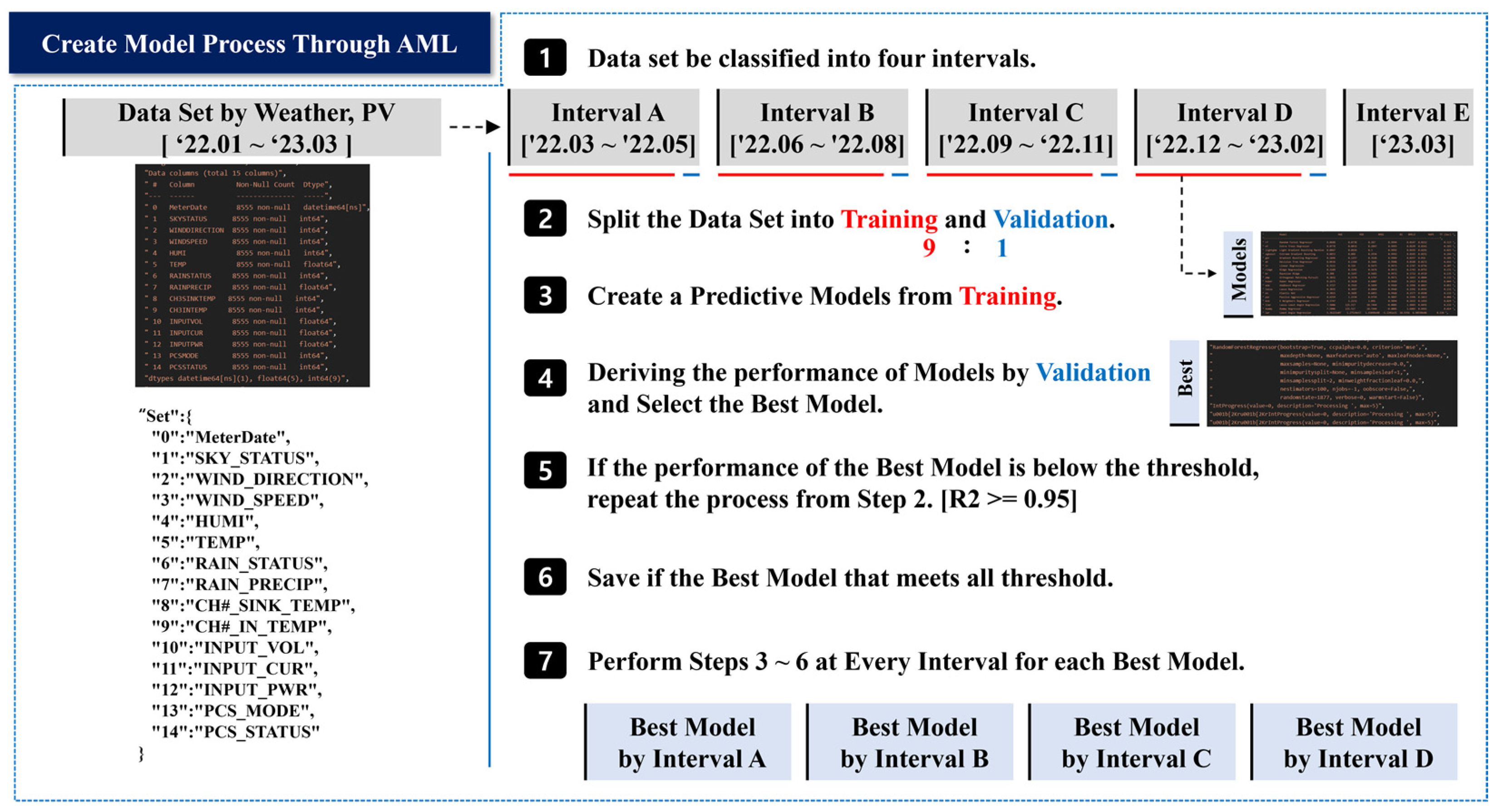
3.2. Process of Creating Models via AML

Accordingly, the process of deriving a solar power generation prediction model using the AML method through the data set obtained earlier is described next like a Figure 4. This process aims to select the best model among the created models after generating several models with the AML method and the dataset. If some of the performance indicators of the best model fall below a certain threshold, the process is repeated [43]. In particular, the R-squared performance determines whether to repeat the process. The R-squared is the ratio between the difference of the target variance and the variance of the prediction error, and the target variance itself. It helps us understand how well the data used in the model-building process fits the regression. R-squared measures how closely the regression predictions approximate the actual values. A higher R-squared score indicates that the model is better at approximating the actual values.

• The period of the obtained dataset is from ‘22.01 to ‘23.03. This period is divided into four seasonal intervals as follows:
  • Interval A [’22.03 to ’22.05]
  • Interval B [’22.06 to ’22.08]
  • Interval C [’22.09 to ’22.11]
  • Interval D [’22.12 to ’23.02]

The unused data for Interval E [‘23.03] are used to verify the actual accuracy by comparing it with the predicted values obtained from the data models generated for the previous Interval A.

2.

Each data interval is divided into training data and validation data randomly in a 9:1 ratio.

3.

The available algorithms are utilized using the training data to create solar power generation models.

4.

The generated models are evaluated using the validation data to derive their performance and compare them to select the best model.

5.

If the best model’s performance falls below a certain threshold for certain metrics, the process is repeated from step 2.

6.

If there is a model that meets all criteria, the algorithms and performance metrics of the prediction models generated concurrently with that model are also checked.

7.

The best prediction models for each interval are derived by executing steps 3 to 6 for all intervals.

By using the above process, it is possible to find the best model for each PV line based on the data characteristics of each interval. Even though the algorithm that demonstrates superior performance may vary for each interval, by using these models, accurate prediction becomes possible [44].

However, this result was obtained using an ideal dataset. In order to apply this process to an actual solar power system, a dataset should be used that excludes data that cannot be obtained in advance [45].

4. Methods—Improving the Accuracy of the Model

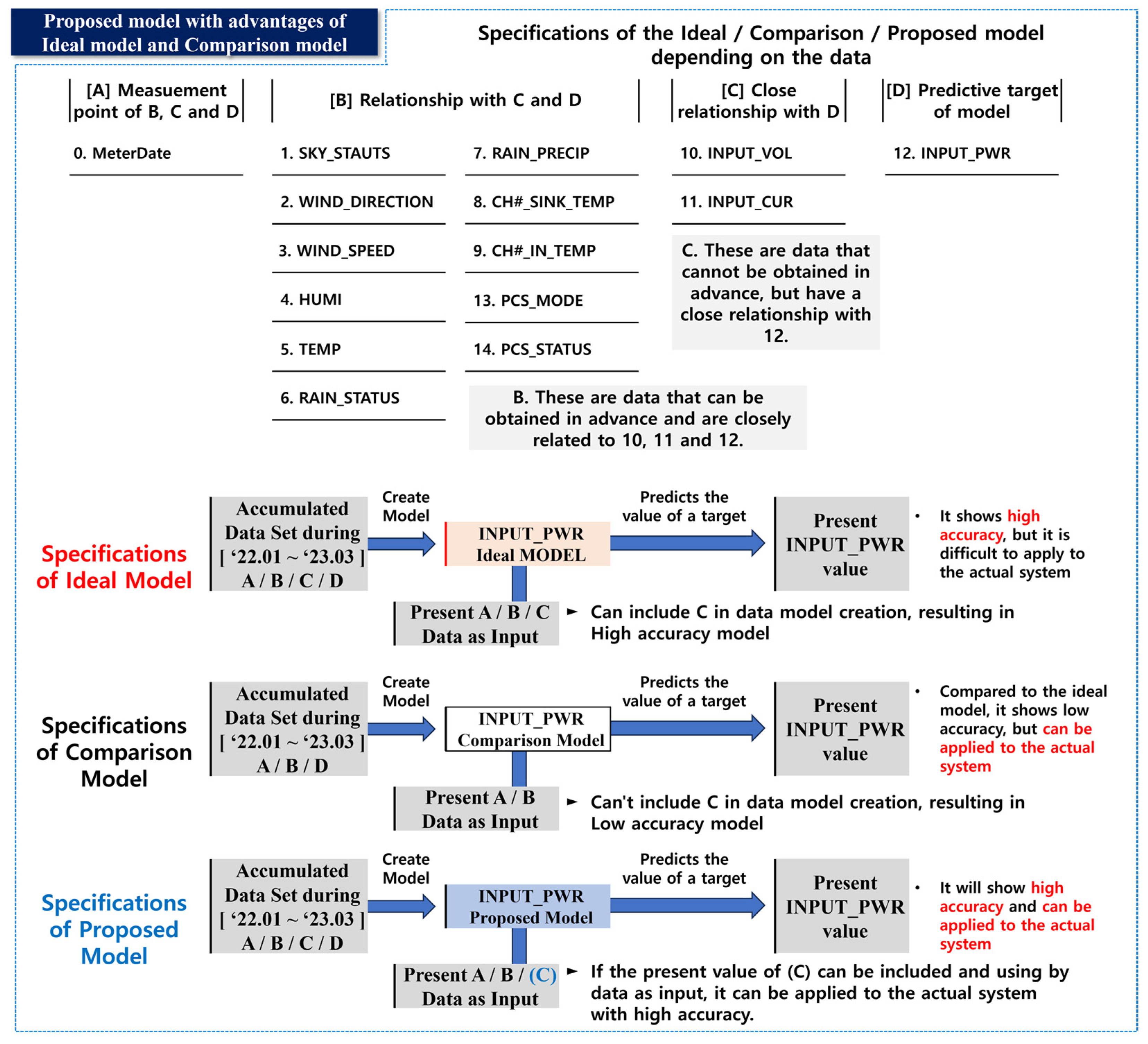
4.1. Relation of Data to Improve Accuracy

The model derived from the dataset that contains all weather and PV data like a Figure 5 is ideal model and not suitable for application to actual solar power systems. This is because some of the data in the dataset cannot be obtained in advance, making it impossible to use them as inputs for the models.

In other words, to create models that can be applied to actual solar power generation systems, it is necessary to exclude some of the data that cannot be obtained in advance from the data set. The following steps like a Figure 6 are taken to create an ideal model, a comparison model, and a proposed model. These models are then compared to find an approach that can be applied to actual solar power generation systems.

We obtained a dataset consisting of 15 data elements for a certain period. Among these, ‘0’ represents the measurement time information. ‘1 to 7’ represent the weather data, more specifically, the weather information (WEATHER). The remaining data are the PV data, where ‘8 to 9’ contain PV sensor information (PV_SENSOR), ‘10 to 12’ represent the PV energy generation information (PV_ENERGY), and ‘13 to 14’ contain the PV status information (PV_STATUS). This process attempts to create a model that predicts the value ‘12’ by including all data in this dataset. We will generate models for each PV line (PV1_IDEAL_MODEL, PV2_IDEAL_MODEL, PV3_IDEAL_MODEL) and classify them as ideal models. Subsequently, the performance indicators of these models are evaluated.

Next, we will create a comparison model (PV1_COMPARISON_MODEL, PV2_COMPARISON_MODEL, PV3_COMPARISON_MODEL) using the information that can be obtained in advance through weather forecasts and PV scheduling operations. It includes data from ‘0 to 7’ (WEATHER) and data from ‘13 to 14’ (PV_STATUS). We then classify these models as comparison models and evaluate their performance indicators. The information used to create the comparison models can be obtained in advance through weather forecasts and schedule-based operational policies. The comparison models are also applicable to actual solar power systems. However, in this paper, to enable higher accuracy than these models, the following approach is applied to create the proposed model and evaluate its performance indicators. It has been observed that the ideal model generated using all weather information and PV data, as shown in Figure 4, exhibits superior performance. Additionally, it has been confirmed that the comparative model derived from available information can be applied to actual solar power generation systems. If the differences in data composition between the ideal model and the comparative model are addressed and utilized to create the model, it would be possible to apply it to actual solar power generation systems like the comparative model and expect higher accuracy. The difference in data composition lies in the presence of PV_ENERGY (‘10’, ‘11’, ‘12’). Among these, ‘12’ is the target for prediction, so obtaining a substitutable value for the actual values of ‘10’ and ‘11’ is necessary.

We examine the relationship between the available information, ‘0 to 7’ (WEATHER) and ‘13 to 14’ (PV_STATUS) like a Figure 7. Regarding the relationship with ‘12’, it is closely linked to ‘10’ and ‘11’. We can identify the following characteristics to confirm the relation between them:

• It can be observed that ‘10’ is closely related to ‘0’ and ‘1’. For example, when it is ‘0’ at sunrise, ‘10’ increases with time, and when it approaches ‘0’ at sunset, ‘10’ decreases. During this process, if ‘1’, the sky status becomes ‘cloudy’, and the fluctuation range of ‘10’ decreases.
• It can be observed that ‘11’ is closely related to ‘10 and 14’. For example, when the value of ‘10’ increases, ‘11’ increases proportionally and remains constant. Conversely, when the value of ‘10’ decreases, ‘11’ decreases proportionally and remains constant. During this process, if the state of ‘14’ is ‘Off’, the value of ‘11’ is fixed at zero.
• It can be observed that ‘12’ is closely related to ‘10’ and ‘11’. ‘12’ is a value that can be derived through the multiplication of ‘10’ and ‘11’. This derived value is affected by the values ‘1 to 7’, ‘8 to 9’, and ‘13 to 14’ and can, therefore, vary accordingly. Through the first condition among the three conditions, it is possible to create a model for predicting ‘10’ using the dataset composed of information that can be obtained in advance. Therefore, it is possible to obtain predicted values for ‘10’ that are similar to the actual values and construct the dataset by replacing the actual values with the predicted values.

Through the second condition, by composing the dataset with information that can be obtained in advance and the values of ‘10’, it is possible to create a model for predicting ‘11’. Similarly, it is possible to obtain predicted values for ‘11’ that are similar to the actual values and construct the dataset by replacing the actual values with the predicted values.

In other words, it is possible to obtain substitutable values for the actual values of ‘10’ and ‘11’ using only the information that can be obtained beforehand.

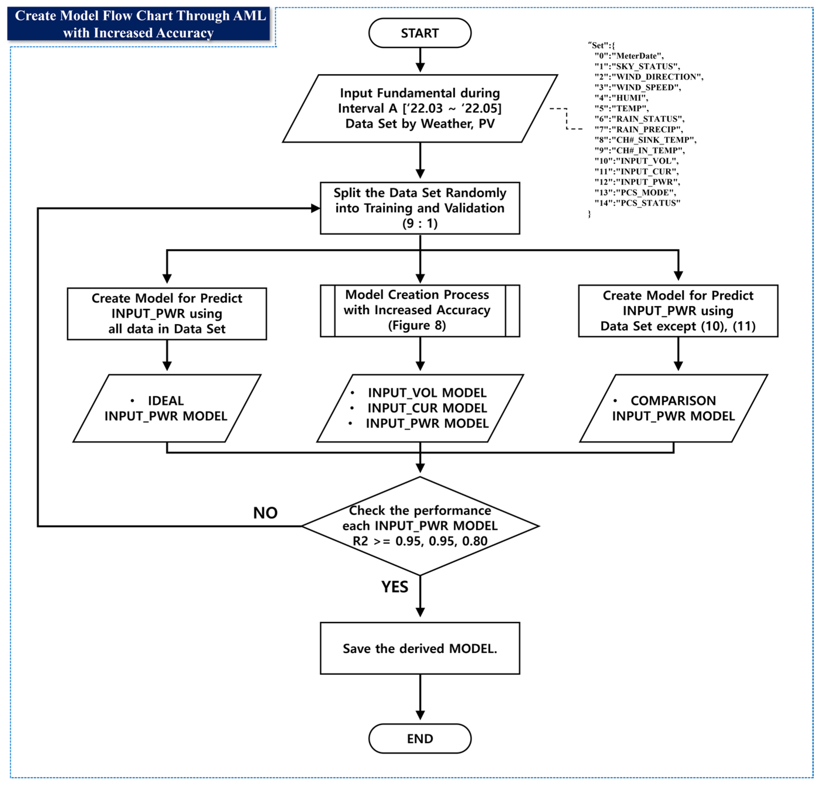
4.2. Process to Improve the Accuracy of the Model

The following process is performed to increase the prediction accuracy of ‘12’ using the above associations, see also Figure 8.

• Check the “Data Set 01”, which includes all data.
• Create a model to predict ‘10’ by excluding ‘11 and 12’ from the original dataset. Obtain the predicted ‘10’ for a specific period.
• Replace ‘10’ in the “Data Set 01” with the predicted values obtained in step (2) to create the “Data Set 02”.
• Create a model to predict ‘11’ by excluding ‘12’ from the “Data Set 02”. Obtain the predicted ‘11’ for a specific period.
• Replace ‘11’ in “Data Set 02” with the predicted values obtained in step (4) to create “Data Set 03”.
• Create a model to predict ‘12’ using the “Data Set 03”. Obtain the predicted values of ‘12’ for a specific period. This is the final prediction for solar power generation.
• Utilize the models generated in steps (2), (4), and (6) as the proposed models, and evaluate their performance using the model obtained in step (6) as the main performance indicator.

The proposed model, as derived using this procedure, can be applied to the actual solar power system, and is expected to perform well, similar to the comparison model. The performance metrics for the ideal model, proposed model, and comparison model can be observed in ‘Results’, and it is anticipated that the performance will follow the order best-performing first: the ideal model, proposed model, and comparison model.

After identifying the creation method for the model using AML and a procedure to apply it to the actual solar power system while improving accuracy, the effectiveness of the proposed approach is validated by implementing all methods in the real system.

5. Methods—Application on an Actual System

The process is divided into two steps to apply both the AML-based prediction model creation method and the procedure to actual solar power systems: Step 1 is “creating a model”, and Step 2 is “predicting the solar power generation”. The purpose of Step 1 is to find the best-performing model that can predict the generated solar power using the AML method by using only data that can be confirmed in advance from the data set.

5.1. Create a Model through AML with Increased Accuracy

The model creation step like a Figure 9 involves creating prediction models for “INPUT_VOL”, “INPUT_CUR”, and “INPUT_PWR” in this order. Next, the purpose of “predicting the solar power generation” is to use the solar power generation prediction model with data that can be checked in advance to find the predicted value for solar power generation at 10-min intervals for the next 24 h.

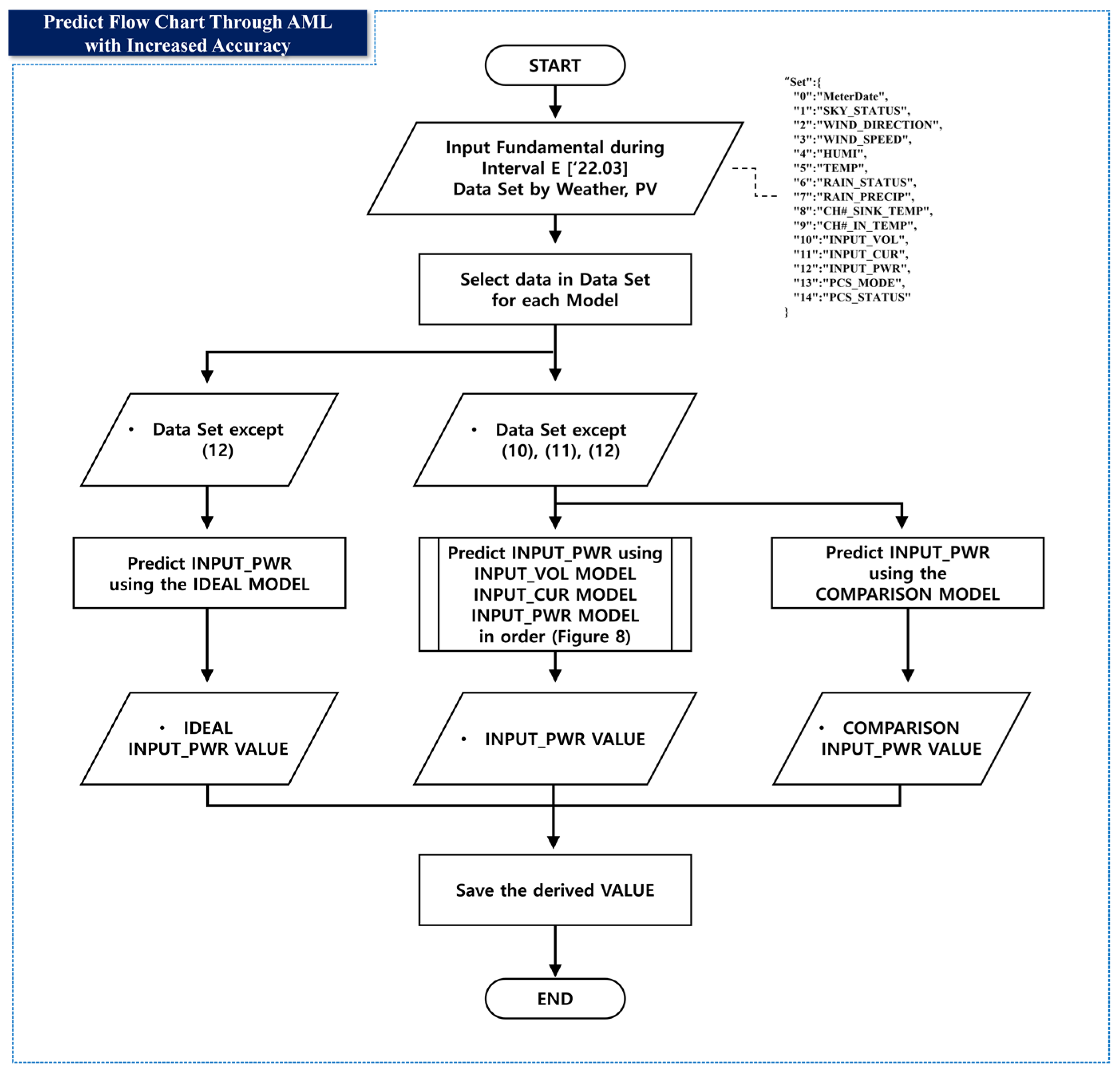
5.2. Predict Value via AML with Increased Accuracy

This step involves finding predicted values like a Figure 10 for “INPUT_VOL”, “INPUT_CUR”, and “INPUT_PWR” in this order. The “creating a model” and “predicting the solar power generation” steps were performed for each PV line, and the results were evaluated.

6. Results

6.1. Performance of Each Model

We used AML to create an ideal model, a proposed model, and a comparison model. Each model aims to predict solar power generation. The proposed model was applied with the accuracy improvement method in Figure 8. The data used for model creation consists of PV data and weather data for each PV line corresponding to “Interval A (‘22.03~‘22.05)” in Figure 4.

Table 5. Performance of the ideal-, proposed-, and comparison- models derived from the PV1 line.

Model	Target	Algorithm	MAE	R2	Training Time [s]
IDEAL MODEL	INPUT_PWR	Bayesian Ridge	0.207	0.997	0.137
PROPOSED MODEL	INPUT_VOL	Random Forest Regressor	14.495	0.976	0.281
	INPUT_CUR	Extra Tree Regressor	1.280	0.934	0.239
	INPUT_PWR	Bayesian Ridge	0.375	0.974	0.134
COMPARISON MODEL	INPUT_PWR	Bayesian Ridge	1.744	0.845	-

presents the performance comparison of three types of models used to predict solar power generation (INPUT_PWR) for PV Line 1. In this table, we can check the algorithms used for each model and their performance metrics based on Mean Absolute Error (MAE) and R-squared score (R2).

A lower MAE and a R2 value closer to ‘1’ indicate superior model performance. The “Training Time” represents the time taken to create each model and is measured in seconds. It is evident from the table that all three types of models were created with a fast speed of under 0.5 s using AML.

Based on Table 5, we can confirm that the model performance for solar power generation prediction in PV Line 1 is superior in the order of ideal model, proposed model, and comparison model. Furthermore, since all the models were created using AML, we can observe that there are differences in the most optimal algorithms employed for each model.

Similarly,

Table 6. Performance of the ideal-, proposed-, and comparison- models derived from the PV2 line.

Model	Target	Algorithm	MAE	R2	Training Time [s]
IDEAL MODEL	INPUT_PWR	Random Forest Regressor	0.05	0.999	0.103
PROPOSED MODEL	INPUT_VOL	Random Forest Regressor	14.435	0.976	0.167
	INPUT_CUR	Random Forest Regressor	1.131	0.925	0.213
	INPUT_PWR	Random Forest Regressor	0.324	0.968	0.223
COMPARISON MODEL	INPUT_PWR	Random Forest Regressor	0.577	0.908	-

and

Table 7. Performance of the ideal-, proposed-, and comparison- models derived from PV3 line.

Model	Target	Algorithm	MAE	R2	Training Time [s]
IDEAL MODEL	INPUT_PWR	Bayesian Ridge	0.007	0.999	0.107
PROPOSED MODEL	INPUT_VOL	Random Forest Regressor	20.520	0.970	0.168
	INPUT_CUR	Extra Tree Regressor	1.864	0.929	0.123
	INPUT_PWR	Random Forest Regressor	0.737	0.977	0.105
COMPARISON MODEL	INPUT_PWR	Bayesian Ridge	0.972	0.920	-

display the performance comparison of the three types of models for predicting solar power generation for PV Lines 2 and 3, respectively. As in Table 5, we can observe that for both PV Lines 2 and 3, the Ideal Model, Proposed Model, and Comparison Model show superior performance in the same order.

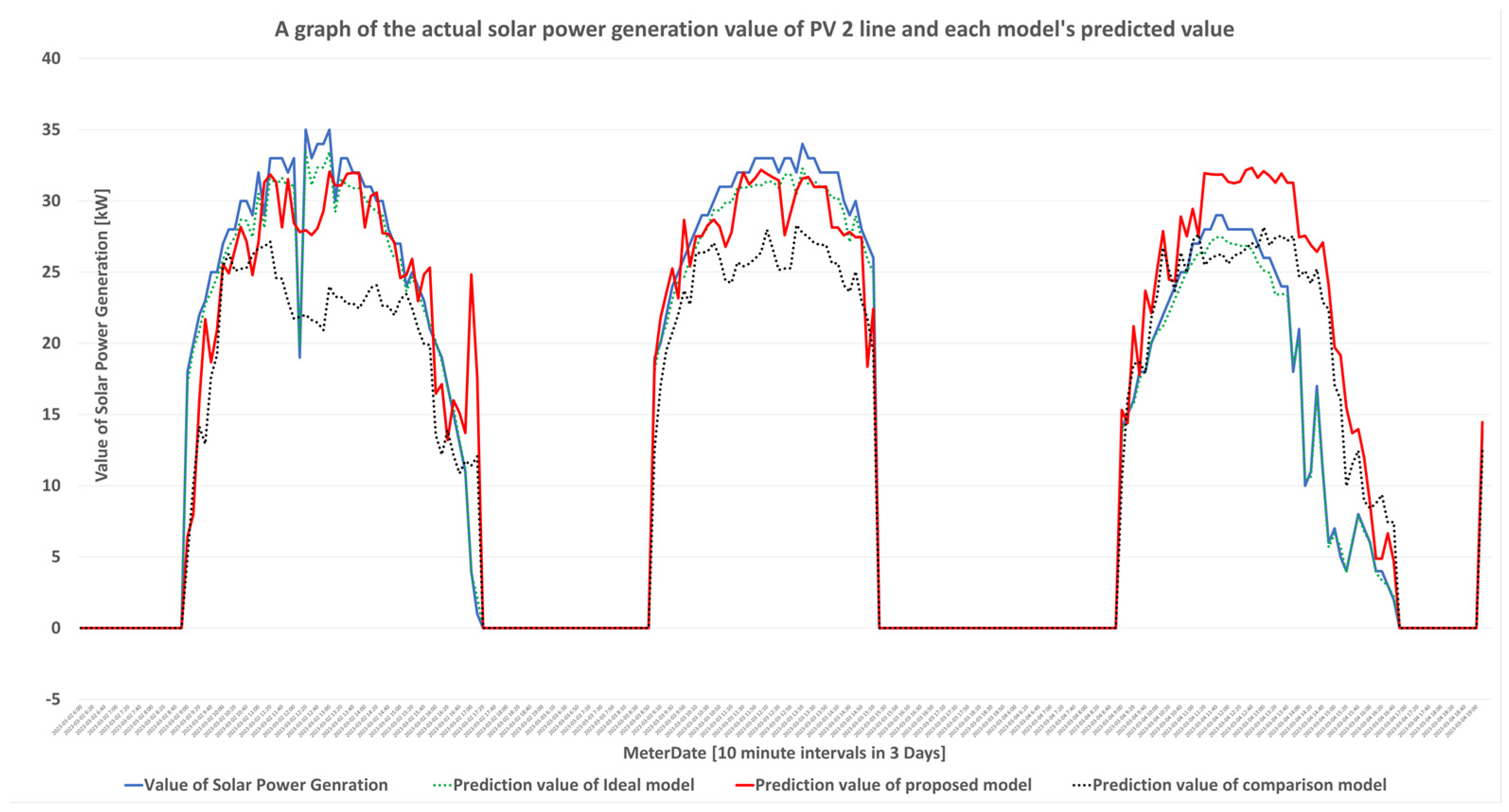
6.2. Prediction Accuracy of Each Model

In Section 6.1, the ideal model, the proposed model, and the control group model were derived using AML using the data of “Interval A (‘22.03~‘22.05)” in Figure 4, and the performance was verified. Similarly, in this section, we check the predicted values through each model and check the validity of the actual model.

The forecast period is “Interval E (23.03)” in Figure 4. Section A and Section E are PV data and weather data with a difference in one year.

Table 8. Comparison between the actual value and the predicted value from the PV1 line.

Model	Average of Predicted Value by the Model	Average of Solar Power Generation Value by PV1	Average of Errors
IDEAL MODEL	20.5092	20.5341	0.3849
PROPOSED MODEL	19.1675		3.2467
COMPARISON MODEL	16.9806		5.3285

is the result of deriving the predicted value of solar power generation in section E through three types of models that predict the solar power generation (INPUT_PWR) of PV line 1 and comparing it with the actual solar power generation predicted value.

The table shows the average amount of solar power generated by PV line 1. Prediction values similar to actual values were derived in the order of the ideal model, the proposed model, and the comparative model. In the case of the comparative model, the error is large compared to the proposed model.

Through

Table 9. Comparison between the actual value and the predicted value from the PV2 line.

Model	Average of Predicted INPUT_PWR Value by the Model	Average of Solar Power Generation Value by PV2	Average of Errors
IDEAL MODEL	18.7010	19.1666	0.5888
PROPOSED MODEL	21.2819		4.2394
COMPARISON MODEL	17.7638		5.6152

and

Table 10. Comparison between the actual value and the predicted value from the PV3 line.

Model	Average of Predicted INPUT_PWR Value by the Model	Average of Solar Power Generation Value by PV3	Average of Errors
IDEAL MODEL	24.3856	24.4906	0.3447
PROPOSED MODEL	23.6446		4.5075
COMPARISON MODEL	25.0363		5.5748

, the models that derived predicted values similar to the actual amount of photovoltaic power generation produced in PV 2 and PV 3 lines were in the order of the ideal model, the proposed model, and the comparison model.

Figure 11, Figure 12 and Figure 13 are a graph showing the actual power generation and predicted values for each model for 3 days (‘23.03.02~‘23.03.04) during Interval E. The period from 19:00 to 06:00, when solar power generation is not performed, was excluded. The blue line represents the actual solar power generation. The green dotted line represents the predicted value of the ideal model. The red line represents the predicted value of the proposed model. The black dotted line represents the predicted value of the comparison model. In all graphs, it can be seen that the red line is more similar to the shape of the blue and green dotted lines compared to the black dotted line.

Through the results section we can finally check the performance of the model and the validity of the predicted value in the order of the ideal model, the proposed model, and the comparative model. As a result, we can confirm that the proposed model is advantageous in predicting solar power generation because it has high accuracy similar to the ideal model and can be applied to actual systems like the comparison model.

7. Conclusions

This paper aims to propose a correct ESG-based operational policy for renewable energy systems, an essential component of zero-energy buildings. To achieve this goal, AML was used to derive a solar power generation prediction method. To do this, PV data from a demonstration site in South Korea was collected and combined with weather data to create the dataset. The proposed prediction model exhibits both actual applicability and high prediction accuracy. In order to validate the superiority of the proposed model, it was compared with the Ideal Model and Comparison Model, and their performance and prediction accuracy were compared.

To enable the proposed method in demonstration sites, we developed a Representational State Transfer Application Programming Interface (REST API). Through this REST API, the zero-energy building’s solar power generation system can make decisions on the individual operations of the three solar power generation lines based on 10-min ahead solar power generation predictions. The operation policy determines whether to operate the solar power generation line to minimize the intervention of the manager of the solar power generation system and maximize energy-saving efficiency.

Through the proposed method, it is expected that renewable energy operational policies for carbon reduction can be derived in zero-energy buildings of various scales and domains. In particular, a demand-oriented operational policy for green energy, such as solar power, could generate surplus electricity. Therefore, this surplus electricity could be applied to building-integrated services such as EV charging platforms. It is anticipated that such integration will contribute significantly to reducing carbon emissions within the building as well as in the city, leading to carbon neutrality.

Moreover, we have prepared another demonstration site in Malaysia so that our proposed method can be applied to the tropical climate of Southeast Asia. The demonstration site is a large 28-floor building located in Kuala Lumpur, Malaysia, and no renewable energy systems are installed. We plan to install a photovoltaic power generation system consisting of a total of 5 PV lines and an Energy Storage System (ESS) on the roof of this building by 2023. In addition, we plan to derive ESG-based operating policies by applying the proposed methods verified in this paper.

References

1. Ahmed, A.; Ge, T.; Peng, J.; Yan, W.-C.; Tee, B.T.; You, S. Assessment of the renewable energy generation towards net-zero energy buildings: A review. Energy Build. 2022, 256, 111755. [Google Scholar] [CrossRef]
2. Vares, S.; Häkkinen, T.; Ketomäki, J.; Shemeikka, J.; Jung, N. Impact of renewable energy technologies on the embodied and operational GHG emissions of a nearly zero energy building. J. Build. Eng. 2019, 22, 439–450. [Google Scholar] [CrossRef]
3. Park, S.; Lee, S.; Park, S.; Park, S. AI-based physical and virtual platform with 5-layered architecture for sustainable smart energy city development. Sustainability 2019, 11, 4479. [Google Scholar] [CrossRef] [Green Version]
4. Li, X.; Lin, A.; Young, C.-H.; Dai, Y.; Wang, C.-H. Energetic and economic evaluation of hybrid solar energy systems in a residential net-zero energy building. Appl. Energy 2019, 254, 113709. [Google Scholar] [CrossRef]
5. Park, S.; Cho, K.; Kim, S.; Yoon, G.; Choi, M.-I.; Park, S.; Park, S. Distributed energy IoT-based real-time virtual energy prosumer business model for distributed power resource. Sensors 2021, 21, 4533. [Google Scholar] [CrossRef]
6. Sharafi, M.; ElMekkawy, T.Y.; Bibeau, E.L. Optimal design of hybrid renewable energy systems in buildings with low to high renewable energy ratio. Renew. Energy 2015, 83, 1026–1042. [Google Scholar] [CrossRef]
7. Derkenbaeva, E.; Vega, S.H.; Hofstede, G.J.; Van Leeuwen, E. Positive energy districts: Mainstreaming energy transition in urban areas. Renew. Sustain. Energy Rev. 2022, 153, 111782. [Google Scholar] [CrossRef]
8. Calise, F.; Cappiello, F.L.; d’Accadia, M.D.; Vicidomini, M. Dynamic modelling and thermoeconomic analysis of micro wind turbines and building integrated photovoltaic panels. Renew. Energy 2020, 160, 633–652. [Google Scholar] [CrossRef]
9. Tamašauskas, R.; Šadauskienė, J.; Bruzgevičius, P.; Krawczyk, D.A. Investigation and Evaluation of Primary Energy from Wind Turbines for a Nearly Zero Energy Building (nZEB). Energies 2019, 12, 2145. [Google Scholar] [CrossRef] [Green Version]
10. Li, M.; Cao, S.; Zhu, X.; Xu, Y. Techno-economic analysis of the transition towards the large-scale hybrid wind-tidal supported coastal zero-energy communities. Appl. Energy 2022, 316, 119118. [Google Scholar] [CrossRef]
11. Brecl, K.; Topič, M. Photovoltaics (PV) system energy forecast on the basis of the local weather forecast: Problems, uncertainties and solutions. Energies 2018, 11, 1143. [Google Scholar] [CrossRef] [Green Version]
12. World Bank. Off-Grid Solar Market Trends Report 2016; An Innovation of the World Bank Group in Cooperation with Global Off-Grid Lighting Association; World Bank: Washington, DC, USA, 2016. [Google Scholar]
13. Park, S.; Park, S.; Yun, S.-P.; Lee, K.; Kang, B.; Choi, M.-I.; Jang, H.; Park, S. Design and Implementation of a Futuristic EV Energy Trading System (FEETS) Connected with Buildings, PV, and ESS for a Carbon-Neutral Society. Buildings 2023, 13, 829. [Google Scholar] [CrossRef]
14. Magrini, A.; Lentini, G.; Cuman, S.; Bodrato, A.; Marenco, L. From nearly zero energy buildings (NZEB) to positive energy buildings (PEB): The next challenge-The most recent European trends with some notes on the energy analysis of a forerunner PEB example. Dev. Built Environ. 2020, 3, 100019. [Google Scholar] [CrossRef]
15. Zero-Energy Building Information Site in Korea Energy Agency. Available online: https://zeb.energy.or.kr/BC/BC00/BC00_01_001.do (accessed on 1 June 2023).
16. Antonanzas, J.; Osorio, N.; Escobar, R.; Urraca, R.; Martinez-de-Pison, F.J.; Antonanzas-Torres, F. Review of photovoltaic power forecasting. Sol. Energy 2016, 136, 78–111. [Google Scholar] [CrossRef]
17. Mussard, M.; Amara, M. Performance of solar photovoltaic modules under arid climatic conditions: A review. Sol. Energy 2018, 174, 409–421. [Google Scholar] [CrossRef]
18. Memiche, M.; Bouzian, C.; Benzahia, A.; Moussi, A. Effects of dust, soiling, aging, and weather conditions on photovoltaic system performances in a Saharan environment—Case study in Algeria. Glob. Energy Interconnect. 2020, 3, 60–67. [Google Scholar] [CrossRef]
19. Li, T.-T.; Wang, K.; Sueyoshi, T.; Wang, D.D. ESG: Research progress and future prospects. Sustainability 2021, 13, 11663. [Google Scholar] [CrossRef]
20. Schram, W.L.; AlSkaif, T.; Lampropoulos, I.; Henein, S.; Van Sark, W.G. On the trade-off between environmental and economic objectives in community energy storage operational optimization. IEEE Trans. Sustain. Energy 2020, 11, 2653–2661. [Google Scholar] [CrossRef]
21. Shi, J.; Lee, W.-J.; Liu, Y.; Yang, Y.; Wang, P. Forecasting power output of photovoltaic systems based on weather classification and support vector machines. IEEE Trans. Ind. Appl. 2012, 48, 1064–1069. [Google Scholar] [CrossRef]
22. Lee, E.S.; Gehbauer, C.; Coffey, B.E.; McNeil, A.; Stadler, M.; Marnay, C. Integrated control of dynamic facades and distributed energy resources for energy cost minimization in commercial buildings. Sol. Energy 2015, 122, 1384–1397. [Google Scholar] [CrossRef] [Green Version]
23. Kim, S.-G.; Jung, J.-Y.; Sim, M.K. A two-step approach to solar power generation prediction based on weather data using machine learning. Sustainability 2019, 11, 1501. [Google Scholar] [CrossRef] [Green Version]
24. Trabelsi, M.; Massaoudi, M.; Chihi, I.; Sidhom, L.; Refaat, S.S.; Huang, T.; Oueslati, F.S. An effective hybrid symbolic regression–deep multilayer perceptron technique for PV power forecasting. Energies 2022, 15, 9008. [Google Scholar] [CrossRef]
25. Khandakar, A.; EH Chowdhury, M.; Khoda Kazi, M.; Benhmed, K.; Touati, F.; Al-Hitmi, M.; SP Gonzales, A., Jr. Machine learning based photovoltaics (PV) power prediction using different environmental parameters of Qatar. Energies 2019, 12, 2782. [Google Scholar] [CrossRef] [Green Version]
26. Park, S.; Park, S.; Choi, M.-I.; Lee, S.; Lee, T.; Kim, S.; Cho, K.; Park, S. Reinforcement learning-based bems architecture for energy usage optimization. Sensors 2020, 20, 4918. [Google Scholar] [CrossRef] [PubMed]
27. Cruz, J.; Mamani, W.; Romero, C.; Pineda, F. Selection of Characteristics by Hybrid Method: RFE, Ridge, Lasso, and Bayesian for the Power Forecast for a Photovoltaic System. SN Comput. Sci. 2021, 2, 202. [Google Scholar] [CrossRef]
28. Shin, D.; Ha, E.; Kim, T.; Kim, C. Short-term photovoltaic power generation predicting by input/output structure of weather forecast using deep learning. Soft Comput. 2021, 25, 771–783. [Google Scholar] [CrossRef]
29. Durrani, S.P.; Balluff, S.; Wurzer, L.; Krauter, S. Photovoltaic yield prediction using an irradiance forecast model based on multiple neural networks. J. Mod. Power Syst. Clean Energy 2018, 6, 255–267. [Google Scholar] [CrossRef]
30. De Leone, R.; Pietrini, M.; Giovannelli, A. Photovoltaic energy production forecast using support vector regression. Neural Comput. Appl. 2015, 26, 1955–1962. [Google Scholar] [CrossRef]
31. Gao, Y.; Li, S.; Dong, W. A learning-based load, PV and energy storage system control for nearly zero energy building. In Proceedings of the 2020 IEEE Power & Energy Society General Meeting (PESGM), Montreal, QC, Canada, 2–6 August 2020; pp. 1–5. [Google Scholar]
32. Bataineh, K.; Dalalah, D. Optimal configuration for design of stand-alone PV system. Smart Grid Renew. Energy 2012, 3, 139. [Google Scholar] [CrossRef] [Green Version]
33. Zamo, M.; Mestre, O.; Arbogast, P.; Pannekoucke, O. A benchmark of statistical regression methods for short-term forecasting of photovoltaic electricity production, part I: Deterministic forecast of hourly production. Sol. Energy 2014, 105, 792–803. [Google Scholar] [CrossRef]
34. Hasan, K.; Yousuf, S.B.; Tushar, M.S.H.K.; Das, B.K.; Das, P.; Islam, M.S. Effects of different environmental and operational factors on the PV performance: A comprehensive review. Energy Sci. Eng. 2022, 10, 656–675. [Google Scholar] [CrossRef]
35. Lu, C.; Li, S.; Penaka, S.R.; Olofsson, T. Automated machine learning-based framework of heating and cooling load prediction for quick residential building design. Energy 2023, 274, 127334. [Google Scholar] [CrossRef]
36. Olsavszky, V.; Dosius, M.; Vladescu, C.; Benecke, J. Time series analysis and forecasting with automated machine learning on a national ICD-10 database. Int. J. Environ. Res. Public Health 2020, 17, 4979. [Google Scholar] [CrossRef] [PubMed]
37. Mahjoubi, S.; Barhemat, R.; Guo, P.; Meng, W.; Bao, Y. Prediction and multi-objective optimization of mechanical, economical, and environmental properties for strain-hardening cementitious composites (SHCC) based on automated machine learning and metaheuristic algorithms. J. Clean. Prod. 2021, 329, 129665. [Google Scholar] [CrossRef]
38. Open Weather Data Portal Site in Korea Meteorological Administration. Available online: https://data.kma.go.kr/cmmn/main.do (accessed on 1 June 2023).
39. Abdul-Rahman, S.; Bakar, A.A.; Mohamed-Hussein, Z.-A. An intelligent data pre-processing of complex datasets. Intell. Data Anal. 2012, 16, 305–325. [Google Scholar] [CrossRef]
40. Berthold, M.R.; Borgelt, C.; Höppner, F.; Klawonn, F. Guide to Intelligent Data Analysis: How to Intelligently Make Sense of Real Data; Springer Science & Business Media: London, UK, 2010. [Google Scholar]
41. Hutter, F.; Kotthoff, L.; Vanschoren, J. Automated Machine Learning: Methods, Systems, Challenges; Springer Nature: Cham, Switzerland, 2019. [Google Scholar]
42. Çetin, V.; Yildiz, O. A comprehensive review on data preprocessing techniques in data analysis. Pamukkale Üniversitesi Mühendislik Bilim. Derg. 2022, 28, 299–312. [Google Scholar] [CrossRef]
43. Hohman, F.; Wongsuphasawat, K.; Kery, M.B.; Patel, K. Understanding and visualizing data iteration in machine learning. In Proceedings of the 2020 CHI Conference on Human Factors in Computing Systems, Honolulu, HI, USA, 25–30 April 2020; pp. 1–13. [Google Scholar]
44. Zhao, W.; Zhang, H.; Zheng, J.; Dai, Y.; Huang, L.; Shang, W.; Liang, Y. A point prediction method based automatic machine learning for day-ahead power output of multi-region photovoltaic plants. Energy 2021, 223, 120026. [Google Scholar] [CrossRef]
45. Chepurko, N.; Marcus, R.; Zgraggen, E.; Fernandez, R.C.; Kraska, T.; Karger, D. ARDA: Automatic relational data augmentation for machine learning. arXiv 2020, arXiv:2003.09758. [Google Scholar] [CrossRef]
Figure 1. Front view of the demonstration site at the Energy Valley Enterprise Development Institute.
Buildings 13 02050 g001
Figure 2. Main manager of the demonstration site’s power control system.
Buildings 13 02050 g002
Figure 3. Schedule manager of the demonstration site’s power control system.
Buildings 13 02050 g003
Figure 4. Illustration of the process to create models via AML using the data set [’22.01~’23.03], and the meaning of # is “PV line number”.
Buildings 13 02050 g004
Figure 5. A data set containing weather and PV data.
Buildings 13 02050 g005
Figure 6. Specifications of ideal model, comparison model, and proposed model.
Buildings 13 02050 g006
Figure 7. Checking of the relation in the data set to improve accuracy.
Buildings 13 02050 g007
Figure 8. Process to improve the accuracy of the proposed model.
Buildings 13 02050 g008
Figure 9. Flow chart for the model creation using AML with increased accuracy, and the meaning of # is “PV line number”.
Buildings 13 02050 g009
Figure 10. Flow chart to predict values using AML with increased accuracy.
Buildings 13 02050 g010
Figure 11. A graph of the actual value of the PV1 line and the predicted value in 3 days.
Buildings 13 02050 g011
Figure 12. A graph of the actual value of the PV2 line and the predicted value in 3 days.
Buildings 13 02050 g012
Figure 13. A graph of the actual value of the PV3 line and the predicted value in 3 days.
Buildings 13 02050 g013