Determination of Final Strand Slips of Prestressed Precast Hollow-Core Slabs Subjected to Flexural Load Using Machine Learning Algorithms

Abstract

Precast prestressed concrete hollow-core slabs (HCUs) are structural elements with less self-weight, providing improved structural effectiveness in withstanding the straining action and allowing for a long span. This study investigated the additional strand slips and developed machine learning (ML) models for evaluating the final strand slips (Śf) of the precast HCUs. Two groups of HCUs, with nominal widths of 1.2 m and 0.55 m, were subjected to flexural loading conditions. One sample from each group was selected to form composite specimens by casting a concrete topping slab, and the restrain mechanism was attached at the ends of the additional HCU specimens. The experimental datasets used to train the ML models, including the support vector machine (SVM), multi-linear regression (MLR), and improved eliminate particle swamp optimization hybridized artificial neural network (IEPANN) models for the prediction of Śf. The efficacy of the IEPANN model compared to the nonlinear predictive models was evaluated, and the performances of the developed ML models were checked using the evaluation matrices. The results indicated that the prestressing strands with relatively higher initial strand slips may result in larger additional slips during flexural loading. The restraining mechanism and cast-in-place topping slab influenced the additional strand slip rate. The hybridized IEPANN model outperformed other classical models in estimating the additional slips with the R² values greater than 0.9 in the two modelling stages, indicating the efficacy of the IEPANN compared to the nonlinear predictive modes.

1. Introduction

Prestressed concrete hollow core slabs (or planks) have been used in many buildings, especially in industrial buildings. The precast slabs are easy to produce and maintain, and cost-effective, and thus, they provide aesthetic architectural values [1]. Less construction time and a high degree of quality can be achieved due to the fast erection time of the precast concrete components and steel frames. Moreover, the usage of hollow-core slabs helps to reduce the dead weight of the structure, which benefits the design of the foundations and columns [2]. Prestressed concrete allows for a longer span than ordinary reinforced concrete.

For certain conditions, machine processes for making HCUs may sometimes prepare concrete with inadequate compaction levels or some paste formation around the pretensioned strand, resulting to a weak bonding capacity, which indicates excessive initial strand slips during the transfer of the prestressing force along the transverse saw-cut precast products. Moreover, the manufacturers often face with the problems of investigating the influence of that slip on the structural capacity of the precast component. Over the decades, several studies have been carried out on the hollow-core slabs [3,4,5,6,7], confirming that excess initial strand slips have significant effects on its capacity. According to Anderson and Anderson [6], the amount of the “free end slip” is strongly correlated to the transfer and flexural bond strength and can be used as a precise indicator of the transfer length when the prestress transfer is considered to be carried out linearly. As a result, the transfer length equation of the ACI 318-83 commentary can be used to directly determine the allowed free end slip [8]. Hence, to limit the prestress transfer length and confirm with the ACI code value, depending on the diameter of the prestressing strands, initial and final levels of prestressing, the equation by Anderson and Anderson [6] restricts the permissible initial strand slips to a range of roughly 1 to 3 mm. Moreover, analytical and prediction equations were developed to evaluate the prestressing transfer length in pretension and prestressing concrete elements [9,10,11,12].

The geometric and material properties are the determining factors for the bond between concrete and steel strands. In many researches, the transfer length of prestressed concrete components is based on the concrete properties and steel geometric properties among the factors affecting the transfer length and bond include the nominal diameter and ultimate tensile strength of prestressing strands, the relationships between the initial and ultimate tensile strengths of prestressing strands, prestressing strand numbers within the member cross-sections, vertical strand spacing, type, length and depth of beam sections, concrete compressive strength at transfer, method of release, beam length, end zone type of the member, amount of fibers in the concrete, coat of strand surface, and type of concrete whether light or normal weight [12,13]. However, it is still unclear how these parameters affects the transfer length, but researchers are still studying some parameters [13]. Several parameters affect the transmission length, including the section size, bond condition, concrete cover, initial or effective prestress, concrete strength, release type, tendon type, the diameter of the prestressing steel, and initial or effective prestress [14,15,16,17,18].

It is clear that several studies have been conducted using AI-based models for engineering problems and yielded a positive results, and individual models had applied to a specific scenario, although there is no superior model applicable to all case studies [19,20,21,22,23,24,25,26]. Therefore, using the concept of ensemble techniques resulting from having more accurate outcomes. The ensemble method have been employed in man engineering field [27,28,29,30,31,32,33]. Dogan and Arslan [34] developed different machine learning algorithms to evaluate punching shear capacities of concrete slabs modified with fiber reinforced polymers and compared the results with the existing building code provision. The authors reported that the prediction values from the building code were more conservative than the experimental results, and the support vector regression (SVR) model outperformed the others five developed model for the prediction of punching shear. Sharghi et al. [35] developed an ensemble model for spatiotemporal assessment of groundwater depletion in semi-arid plains. Chou and Nguyen [28] predicted the mechanical properties of reinforced concrete using metaheuristics-optimized ensemble techniques and reported that the technique was highly promising for predicting the structural behaviors of reinforced concrete beams. Liang et al. [29] developed three ensemble models, including Random Forest (RF), Extreme Gradient Boosting Machine (XGBoost), and Light Gradient Boosting Machine (LGBM), for modeling the creep behaviors of concrete. Nageh et al. [36] selected optimum variables for the classification of failure patterns of RC bridge columns. Joo et al. [11] proposed an analytical model to predict the shear strength of prestressing HCUs containing core-filling concrete and calculated the shear demand of prestressed HCUs and filled cores based on the nonlinear flexural analysis. The results indicated that the shear strength decreased with the stiffness of the interfacial shear stress–slip relationship between the HCU and filled core reduced. Moreover, the developed model predicted the shear contribution of HCUs and filled core. Arslan et al. [37] carried out experimental and numerical studies on the reinforced concrete slabs to investigate the effects of plastic circular balls placed in the midsection of reinforced concrete slabs. Basic parameters including strength, thermal ductility, and acoustic performance were investigated in the study. Dang et al. [12] estimated the transfer length (TL) of a prestressed concrete strand, which was determined using concrete surface strain together with the maximum strain method. It was deduced from this work that ACI and AASHTO codes can be used for the estimation of the TL. Kankeri et al. [38] developed a finite element model to predict the precracked behaviors of HCUs strengthened with near-surface mounting. Alhassan et al. [13] used ANN techniques on prestressed concrete stands, which is presently the only literature available during this research that studied prestressed strands using ANN model. Souza et al. [39] analyzed the shear strength of prestressed HCUs supported on shallow beams using a computational model. The parametric investigation was also conducted to determine the infill effects of the hollow core ends and the support stiffness of steel beams on the shear capacity of slabs. Abdelatif et al. [40] developed models to stimulate the prestress transfer forces from reinforcing and prestressing steel in pretensioned concrete elements. Therefore, investigating the addition strand slip in precast prestressed HCU under high-intensity loads, as in the case of parking places and bridges is essential. The main aim of this study is to evaluate the final prestressed strand slips of precast concrete hollow-core slabs subjected to flexural loading. The additional strand slips at the two ends of HCUs due to the application of flexural loadings were experimentally measured, and then the final strand slips were computed. Moreover, the application machine learning algorithms, including the hybrid model, namely the improved eliminate swam particle optimization hybridized artificial neural network (IEPANN) and classical models, such as support vector machine (SVM) and multilinear regression (MLR), were employed to predict the final strand slips. The prediction skills can prevent the need for conducting high-cost experiments and save time.

2. Strand Slip Theory

Section 12.9 of ACI 318-83 Building Code Requirement for Reinforced Concrete [8] specified that development length l_d should not be less than

$$l_d=(f_{ps}-2\frac{f_{ps}}{3})d_b$$

(1a)

The equation can be simplified as

$$l_d=l_t+l_b=\frac{f_{ps}}{3}{d}_b+(f_{ps}-f_{se})d_b$$

(1b)

where l_t denotes the prestress transfer length, l_b is the flexural bond length, l_d is the development length based on the ACI code, d_b is the nominal diameter of prestressing strands, f_ps is the stress in prestressing strands after transfer, and f_se is the effective stress in prestressing strands.

Therefore, large initial end slips are the results of the transfer of prestress forces, and thus, a large length may occur. However, strand slip theory assumes that the initial strand slip from the concrete saw-cutting face translates the concrete bond quality. Hence, the transfer length and flexural bond are closely correlated with the end slip. The recorded initial end slip (σ) is associated with the strand force by assuming a linear increment of the force, as depicted in Figure 1. The average force of the prestressing strands in the transfer area, P_t(aveg) = P_t/2, is associated with the end slip through the strand strains

$$\sigma =\frac{P_{t(averg)}{l}_i}{A_{ps}E}=\frac{P_t{l}_i}{2A_{ps}E}$$

(2)

where A_ps is the area of strand in the tension zone, E is the elastic modulus of prestressing strands, σ is the recorded initial slip at the end of the HCU, and P_t is the maximum force in strands following transfer.

By rearranging Equation (2) and including the steel stress $f_{st}=P_t/A_{ps}$, the transfer length can be expressed as

$$l_i=\frac{2\sigma A_{ps}E}{P_t}=\frac{2\sigma E}{f_{st}}$$

(3)

When l_i from Equation (3) is greater than l_t from Equation (1b), it can be assumed that the strand end slip is higher than the allowable value, (σ_all) and it can be found by equating l_t to l_i

$${\sigma }_{all}=\left(\frac{1}{6}\right)\frac{f_{se}{f}_{st}{d}_b}{E}$$

(4)

The allowable end slip is described as the initial strand slip at the saw-cut end of the hollow-core slab, resulting in a transfer length equivalent to that calculated by the steel stress.

3. Materials and Methods

3.1. Materials

3.1.1. Precast Prestress Concrete HCU

The prestressed concrete HCUs used in this study were obtained from the local precast concrete manufacturer in Ankara, Turkey. Two different sizes of HCU specimens were adopted in this study, three HCU samples with a nominal width of 1200 mm and two HCU samples with a nominal width of 550 mm, and all the HCUs had a depth of 150 mm, pretensioned with 9.5 mm diameter 7-wire strands. The HCU specimens with the 1200 mm width were reinforced with 8 No. of prestressing strands, while the narrow specimens were reinforced with 4 No. of prestressing strands, as shown in Figure 2.

Table 1. Properties of Hollow-Core Units.

Specimen ID	No. of Prestressing Strands	Specimen Width (mm)	Cast-in-Place Slab	Depth of Cast-in-Place Slab (mm)
HCU-WB	8	1200	-	-
HCU-WT	8	1200	Yes	50
HCU-WT-R *	8	1200	Yes	50
HCU-NB	4	550	-	-
HCU-NT	4	550	Yes	50

* Two ends of the cast-in-place concrete in the specimens were restricted. HCUs with W represent the specimens with 1.2 m width, N represents the specimen with a narrow width of 0.55 m, and the specimens attached with T and B were tested with and without topping slab, respectively.

summarizes the physical properties of the HCU specimens used in this study, and the geometric details are depicted in Figure 2.

3.1.2. Cast-in-Place Concrete Topping

Ordinary Portland cement (Grade 42.5R) was used to prepare the concrete with target compressive strength of 30 MPa, cast on the top of the machine-finished surface of the precast prestressed HCUs to serve as the topping slab to form the composite specimens. For this reason, three specimens were selected from the two groups. To achieve sufficient bond strength at the interface between the HCUs and concrete topping slabs, the top surfaces of the HCUs were cleaned adequately using compressed air and slowly applied water to provide moist conditions. The mix w/c ratio of 0.5 was adopted for the concrete. To prevent crack propagation and temperature effect, cast-in-place topping slabs were reinforced and 6 mm diameter steel bars were placed at 150 mm center to center inside the concrete.

Table 2. Mix design of the topping slabs.

Material	Sand	Medium Aggregate	Coarse Aggregate	Cement	Water	Superplasticizer
Amount (kg/m3)	900	600	400	400	200	3

shows the mixed proportion of the cast-in-place concrete topping slab. The natural river sand with a maximum particle size of 4.75 mm was used as fine aggregate. The coarse aggregate and medium size aggregates were obtained from crushed natural stone. Coarse aggregate had a maximum particle size of 16 mm, while the medium size aggregate had a particle size ranging between 5 mm to 9.5 mm. To prepare a cast-in-place top slab, smaller particle size aggregates were essential in achieving better bond strength at the interface of the composite specimens. Therefore, medium-size aggregates were introduced in the mix with a higher amount than coarse aggregate, as shown in Table 2.

3.2. Testing Procedure

The HCU specimens were subjected three-point bending, and the load was applied at the midpoint of the 4.6 m span. The applied load was distributed throughout the whole width of the sample using a steel spreader beam, and roller supports were attached at each end of the span. The experimental test setup for determining the additional strand is depicted in Figure 3. To achieve a uniform load transmission from the spreader beam to the HCU test samples, a strip of neoprene pad was placed between the spreader beam and the top surface of the specimens. A 300 kN hydraulic jack with a load cell and a swivel mechanism was fixed on the top of the spreader beam to apply the load under load-controlled conditions. Tests were conducted using the step force loading that increased gradually until failure. Each load step had a 10 kN, and each step had some holding time after loading.

The HCUs were equipped with displacement meters, and a data collecting system was employed to simultaneously record the data from the displacement transducers and the load cell during the load testing. To measure the deflection, two displacement transducers were positioned at the midspan. Four displacement transducers were placed at each end of specimens to measure the additional strand slips during the load tests, as shown in Figure 3. Moreover, restraining devices were installed to the two ends of the HCU-WTR specimens using steel channel sections and clamped on the top and bottom surfaces of the specimens to control the relative slides between the topping slab and the HCUs. Steel plates and threaded rods were employed to provide restraints against the slips of the concrete topping slabs. Finally, the flexural load was steadily applied to the test specimens until they completely failed in flexure, with evident extensive cracks on the test specimens.

4. Artificial Intelligent-Based Model

This study applied two classical ML models, including SVM and MLR. Moreover, an optimization algorithm referred to as the improved eliminate particle swamp optimization (IEPSO) was applied to improve the weight and bias of the ANN model and transformed to a hybrid model called IEPANN. Both classical and hybrid models employed to train and test experimental datasets. The datasets were randomly arranged and split into training and testing portions. The training set accounted for 70%, and the remaining was used for testing. The experimental dataset for modelling the final strand slips included the ultimate load, initial deflection, cross-sectional area of the strand, HCU width, and initial strand slip as the potential input parameters, while the final strand slip was simulated as the output parameter, as shown in

Table 3. Descriptive statistic dataset.

Direction	Parameter	Symbols	Unit	Min	Max	Mean	SD	Kurtosis	Skewness
Inputs	Ultimate load	Pult	kN	26.300	83.700	62.263	19.305	−0.773	−0.649
	Initial deflection	δcr	mm	4.200	8.400	6.295	1.386	−0.851	−0.339
	Area of strand	As	mm2	219.20	438.40	383.60	95.667	−0.622	−1.182
	Width of HCU	b	m	0.550	1.200	1.037	0.284	−0.622	−1.182
	Initial strand slip	Śi	mm	0.00	21.00	2.932	3.536	13.180	3.462
Output	Final strand slip	Śf	mm	0.100	24.90	4.205	5.046	7.264	2.725

.

4.1. Artificial Neural Network (ANN)

The ANN is a machine learning model for data analysis using a decision-layers network. This ML comprises a processing element set connected by a synaptic weight known as neurons. As seen in Figure 4, the ANN model structures consisted of input, hidden, and output layers. The output for the neurons was produced by multiplying the inputs by a modified weight and sending it through a transfer function [41]. The network trained the dependent and independent parameters, and thus the best weight was computed through the learning practice. Figure 4a shows the neurons that collect the input out parameters, and the Net is the sum of the computed weight and bias in the individual neuron, which can be expressed as [42].

$$Net={\displaystyle \sum _{i=1}^n{w}_{ij}{x}_i+b_i}$$

(5)

The hyperbolic tangent function was used for better prediction skills. It has function values from −1 to 1, and it is given in Equation (6).

$$y=f(Net)=\frac{2}{1+e^{-2net}}-1$$

(6)

The technique is applied to each layer of the multilayer perception until the output signal in the final layer is obtained. The weights and biases in the whole multilayer perception are updated to compute and minimize the errors of the ANN.

4.2. Support Vector Machine (SVM)

SVM is the machine learning model capable of obtaining reliable solutions to prediction, classification, regression, and pattern recognition [43]. It was invented by Cortes and Vapnik (1995), and the model was characterized by two essential functions, including risk minimization and statistical learning theory, which make it excellent from other artificial intelligent models. There are four alternative approaches utilizing kernel functions in SVM, including linear, sigmoid, polynomial, and radial basis functions. Due to the robustness of the kernel function to simulate complex nonlinear functions [44], it was applied in our study. In the SVM, linear regression was fitted on the data where the nonlinear data were obtained in a nonlinear kernel. The data set is given by $\left\{\left(x_i,d_i\right)\right\}$ ${}_i^N$ where x_i is the input vector, d_i is the actual value, and N is the total number of data patterns. Equation (1) presents the general Support Vector Machine’ function:

$$y=f(x)=w\varphi (x_i)+b$$

(7)

4.3. Multilinear Regression (MLR)

MLR estimates the linear regression between the dependent variable, expressed as y, y ϵ Rⁿ $\times$ 1, and the independent variables expressed as X, X ϵ Rⁿ $\times$ ^m [45]. Equation (8) present the mathematical expression of MLR model.

$$y=c_0{x}_0+c_1{x}_1+c_2{x}_2\dots \dots .c_n{x}_n={\displaystyle {\sum }_{i=1}^n{c}_i{x}_i=c^{T}x}$$

(8)

where $c_0$ $c_1$…. $c_n$ are the partial regression coefficients of the model. The solution of the MLR model follows the least-square method presented in Equation (9). However, the fitness of the model was determined by squaring the difference between the measured value Z and the value predicted.

$$Z={(y-Xc)}^T(y-Xc)$$

(9)

4.4. Improved Eliminate Particle Swarm Optimization (IEPSO)

The improved eliminate particle swarm optimization was invented by Lv et al. [46] following the principle of last-eliminate to improve the personal–global information sharing capacity and global optimization efficacy. IEPSO is an extension of the standard PSO. Similar to the standard PSO, Equation (9) expressed the updated positions and velocities of individual particles in the solution space.

$$V_{ij}^{k+1}=\underset{\mathrm{Standard} \mathrm{PSO}}{\underbrace{w{V}_{ij}^k{c}_1{r}_1(p_{bestij}^k-X_{ij}^k)+c_2{r}_2(G_{bestij}^k-X_{ij}^k)}}+\underset{{\varphi }_3}{\underbrace{c_3{r}_3\left|G_{bestij}^k-p_{ij}^k\right|}}$$

(10)

The standard PSO algorithm updated velocity is represented in the terms shown in Equation (10). The term ϕ₃ is the PSO extension, known as the personal–global information sharing term. In contrast to the normal PSO, the IEPSO is not restricted to only one-way information exchange between the individual particles and the global best particles. The value of c₃ was chosen based on two criteria. If c₃ is assumed to be a constant, then c₃ = 2. Equation (11) is used to determine c₃ when continuous values are assumed.

$$c_3=k\left[\left(c_{3i}-c_{3j}\right)\times \frac{t}{t_{\max }}\right]$$

(11)

where k has defined the controlling factor, and has values of −1 and +1 for linearly increasing and linearly decreasing functions, respectively, c_3i is the initial value of c₃, c_3j is the stopping value of c₃, t represents the iteration number, and t_max is the peak number of iterations.

4.5. Improved Eliminate Particle Swamp Optimization Hybridized Artificial Neural Network (IEPANN)

The IEPANN is a hybrid model established through the optimization process of the ANN and IEPSO to estimate the final prestressing strand slip subjected to three-point bending loading. The experimental dataset was split into training and testing sets. The normalization process was performed on the dataset to improve its integrity and remove the inconsistency-related dimensions among the datasets. Equation (12) was used for normalization techniques.

$$y_{norm}=\frac{y-y_{\min }}{y_{\max }-y_{\min }}$$

(12)

where $y_{norm}$ donates the normalized data value, $y$, $y_{\min }$, and $y_{\max }$ are the observed, maximum and minimum data, respectively.

In addition, Equations (9) and (10) present the modelling method of the IEPANN technique, which is systematically illustrated in Figure 5, and is used to train the ANN through the IEPSO. Initializing random particles was the first step in the learning process. and their positions are representatives of the weight and bias of the ANN, which are randomly allocated. The IEPANN is trained based on the initial weight and bias, and thus computes the MSE between the measured and predicted parameters. The model efficacy was enhanced by modifying the particle positions and reducing the MSE gently in each iteration. P_best and G_best are chosen to determine and update new velocities in each iteration. The inferior particles are removed and substituted with the new ones if the revised velocities V_i^k+1 and X_i^k+1 surpass the boundary range. The optimization process is conducted in accordance with the procedure until the termination requirements are satisfied. Lower MSE or maximum iterations could be the criteria for stopping. The model performance depends heavily on the choices of the hidden layers and neurons. Some studies [47,48] suggest that a hidden layer is effective for a different regression model, although there is no precise technique for determining the number of the hidden layers in the ANN model.

4.6. Evaluation Matrices

Five performance indicators were used in this study to assess the AI-based model performance. These included R², MAE, RMSE, MAPE, and RI, as summarized in

Table 4. Evaluation matrices.

Matrix	Formula	Description
R2	${\left[\frac{{\displaystyle {\sum }_{i=1}^n(q_i-\overline{q})(p_i-\overline{p})}}{{\displaystyle {\sum }_{i=1}^n(q_i-\overline{q}{)}^2{\displaystyle {\sum }_{i=1}^n{(p_i-\overline{p})}^2}}}\right]}^2$	R2 is frequently used as a performance metric to describe how well a model predicts a given variable. Its value is a number between 0 and 1 [21,24].
MSE	$\frac{1}{n}{\displaystyle {\sum }_{i=1}^n{(q_i-{\overline{q}}_i)}^2}$	The statistical inaccuracy demonstrates the effectiveness of the model. High prediction accuracy is indicated by the MSE value being close to zero.
RMSE	$\sqrt{\frac{1}{n}{\displaystyle {\sum }_{i=1}^n{(q_i-p_i)}^2}}$	This shows the difference between the predicted and observed values. When the RMSE value approaches 0, better performance is attained.
MAPE (%)	$\frac{1}{n}{\displaystyle {\sum }_{i=1}^n\left|\left.\frac{p_i-y_i}{y_i}\right|\right.}\times 100$	This presents the percentage errors, the MAPE shows how well the model could forecast the observed values. The lower percentage shows a more accurate algorithmic prediction [49].
RI	$\frac{MAE+RMSE+MAPE}{3}$	RI is a function of three errors that have been standardized.

. As a result, the best developed model is selected based on the accuracy level noted in the aforementioned matrices.

5. Results and Discussion

5.1. Failure Modes of the HCUs

Figure 6 shows the failure modes of the HCUs under three-point bending tests. The hollow-core unit typically developed a minor first crack under loading conditions towards the bottom of the loading point. The tension zone developed additional cracks as the load increased. On continuous loading, concrete crushing occurred in the upper portions of the HCUs, close to the midspan section, until the HCUs completely failed. At this point, non-composite specimens (HCU-WB and HCU-NB) revealed web shear failure, as shown in Figure 6a,b. The HCU specimens with concrete topping slabs (composite HCUs) exhibited excessive slips at the interface, as shown in Figure 6b,d. Additionally, on each side of the composite specimen at the maximum cracking force, vertical separations between the HCU and topping slab occurred. At the same time, the other side did not reveal vertical separations. The vertical separations in the HCU-NT specimens were more pronounced than those in the HCU-WT specimens. This is may be attributed to the widths of the specimens.

5.2. Additional Strands Slip

The strand slips at the ends of HCUs were noticeable before loading. These strand slips can be obtained on the prestressing members under a non-serviceability state, and they occurred during the saw-cut of prestressing members, which are referred to as the initial slips. Past studies suggested that high initial strand slips are an indication of low concrete quality and inadequate compaction level, which lowers the flexural and shear strength of HCUs [50,51]. Before loading the HCU specimens, the initial strand slips after the saw-cut from the manufacturer were measured at the ends of HCUs. The final prestressing strand slips were determined at the two ends of individual prestressing strands in the HCU specimens. The initial slip values in most of the strands were in the range of 2 and 3 mm. However, an initial strand slip of 21.0 mm was obtained in one of the strands of the HCU-WB specimen at the south end with a peak final slip of 24.9 mm. The knowledge of prestressing strand slips is typically restricted to free-end slip measurements that are utilized to calculate the transmission length using Guyon’s theory [52]. The results indicated that the prestressing strands with relatively higher initial strand slips may result in larger additional slips during flexural loading. The additional strand slips were computed at the two ends (south end and north end) as specified in Figure 3, displaying the instrumentation of the strands at the south ends. From Figure 7, it can be seen that the prestressing strands in the HCU samples exhibited difference levels of additional slips due to the existing initial slips. The HCU-WB specimens exhibited a maximum average additional slip of 4.49 mm at the south ends for all HCU specimens. Some specimens showed greater additional slips at one end compared to the other end, as shown in Figure 7a. The additional strand slips for all strands at the south end were higher than those of the corresponding north end. In contrast, the additional strand slip values at the south end of the HCU-WTR specimens were higher than those of the north end. Some specimens demonstrated comparatively equal additional strand slips at the two ends in most of the prestressing strands, as indicated in Figure 7b,e. Moreover, prestressing strands in specimen HCU-NT revealed no additional strand slips at the ends of the majority of its strands.

Figure 8 shows the relationships between the additional strand slips and midspan deflections for the five testing conditions. The plots represent other strand slips, and one prestressing strand from each specimen was considered. The developments of strand slips varied according to the testing conditions during loading. From Figure 8a, at the initial loading, the slip increased gradually with the increasing deflection until the initial crack occurred, and then the strand slip increased rapidly with the increasing deflection. The horizontal line appeared in the strain slip vs. deflection curve shown in Figure 8a was due to the sudden released of the applied load, and this did not affect the overall results. The effect of the topping slab on the strand slip was noticed on the HCU-WT specimen. In this specimen, the additional strand slip was not effective until the specimen reached a significant deflection level. After that, rapid strand slip occurred due to the loss of the bond strength between the HCU and topping slab, as shown in Figure 8b. The HCU specimen restrained at its two ends displayed a systematic increase in the strand slip. The strand slip was observed when the deflection was about 40 mm, and then the slip continued to increase with the increasing deflection until the complete failure of the specimen. The maximum slip value of 9.1 mm was recorded in the strands considered for HCU-WB, which was 139.5% and 184.4% higher than those of the strands in the HCU-WT and HCU-WTR specimens, respectively. This result indicates that the topping slab and restrain mechanism significantly affected the slip values obtained in the prestressing strands when subjected to loading conditions. In addition, this also determines the load carrying capacity of the structures.

Figure 8d,e show that sudden slips were obtained in the strands considered for the HCU-NB and HCU-NT specimens. Due to the smaller width of the specimens, both HCU-NB and HCU-NT specimens demonstrated sudden strand slips. As can be seen, maximum slip values recorded on these strands were very small, approximately less than 0.2 mm in the failure stage of the specimens. Generally, comparing the narrow specimens (HCU-NB and HCU-NT) with larger specimen widths (1.2 m), it can be noted that higher strand slip values were obtained in the prestressing strands of the HCU-WB, HCU-WT, and HCU-WTR specimens, exhibiting higher load-carrying capacities. The performance properties of non-composite specimens are summarized in

Table 5. Performance properties based on the experimental results of the HCU-WB specimens.

Properties	Symbol	Calculated Value	Unit
Area	A	113,300	mm2
Moment of inertia	I	289.8 $\times$ 106	mm4
Modulus of elasticity	E	31,000	MPa
Top centroid	yt	76.6	mm
Bottom centroid	yb	73.4	mm
Eccentricity	e	23.4	mm
Transformed moment of inertia	Itr	291 $\times$ 106	mm4
Area of steel	As	438.4	mm2
Initial prestressing after losses	p	550	kN
Initial prestressing force	fPi	611.5	kN
Stress in prestressing steel in flexure	fps	1718	MPa
Initial cracking load	Pcr	34	kN
Cracking moment	Mcr	39.1	kNm
Ultimate load capacity	Pult	51	kN
Deflection at cracking load	δcr	7.6	mm
Max deflection	δmax	157.6	mm
Interface slip at max. deflection	Ɛ	13.7	mm
Compressive strength	CS	30	MPa
Interface shear strength	τ	0.22	MPa

and

Table 6. Performance properties based on the experimental results of the HCU-NB specimen.

Properties	Symbol	Calculated Value	Unit
Area	A	56,700	mm2
Moment of inertia	I	138.3 $\times$ 106	mm4
Modulus of elasticity	E	31 $\times$ 103	MPa
Top centroid	yt	73	mm
Bottom centroid	yb	77	mm
Eccentricity	e	27	mm
Transformed moment of inertia	Itr	139.3 $\times$ 106	mm4
Area of steel	As	219.2	mm2
Initial prestressing after losses	p	258.13	kN
Initial prestressing force	fPi	305.78	kN
Stress in prestressing steel in flexure	fps	1395	MPa
Initial cracking load	Pcr	13.4	kN
Cracking moment	Mcr	34.4	kNm
Ultimate load capacity	Pult	26.3	kN
Deflection at cracking load	δcr	6.3	mm
Max deflection	δmax	165	mm
Interface slip at max. deflection	Ɛ	13.7	mm
Compressive strength	CS	30	MPa
Interface shear strength	τ	0.26	MPa

, which shows the observed physical and flexural characteristics of the HCUs obtained from the experimental program.

6. AI-Based Modelling Results

AI-based model is the most widely used technique for solving several engineering problems, such as classification, prediction, pattern recognition, and regression problems. With the aid of a predetermined architecture, an AI-based model was used to develop predictions based on the input data and learning type. This study compared the efficacies of the two classical models (MLR and SVM) and the hybrid IEPANN model for predicting the final prestressed strand slips of precast prestressed HCU specimens under flexural loading conditions.

6.1. Optimal Input Parameters Selection

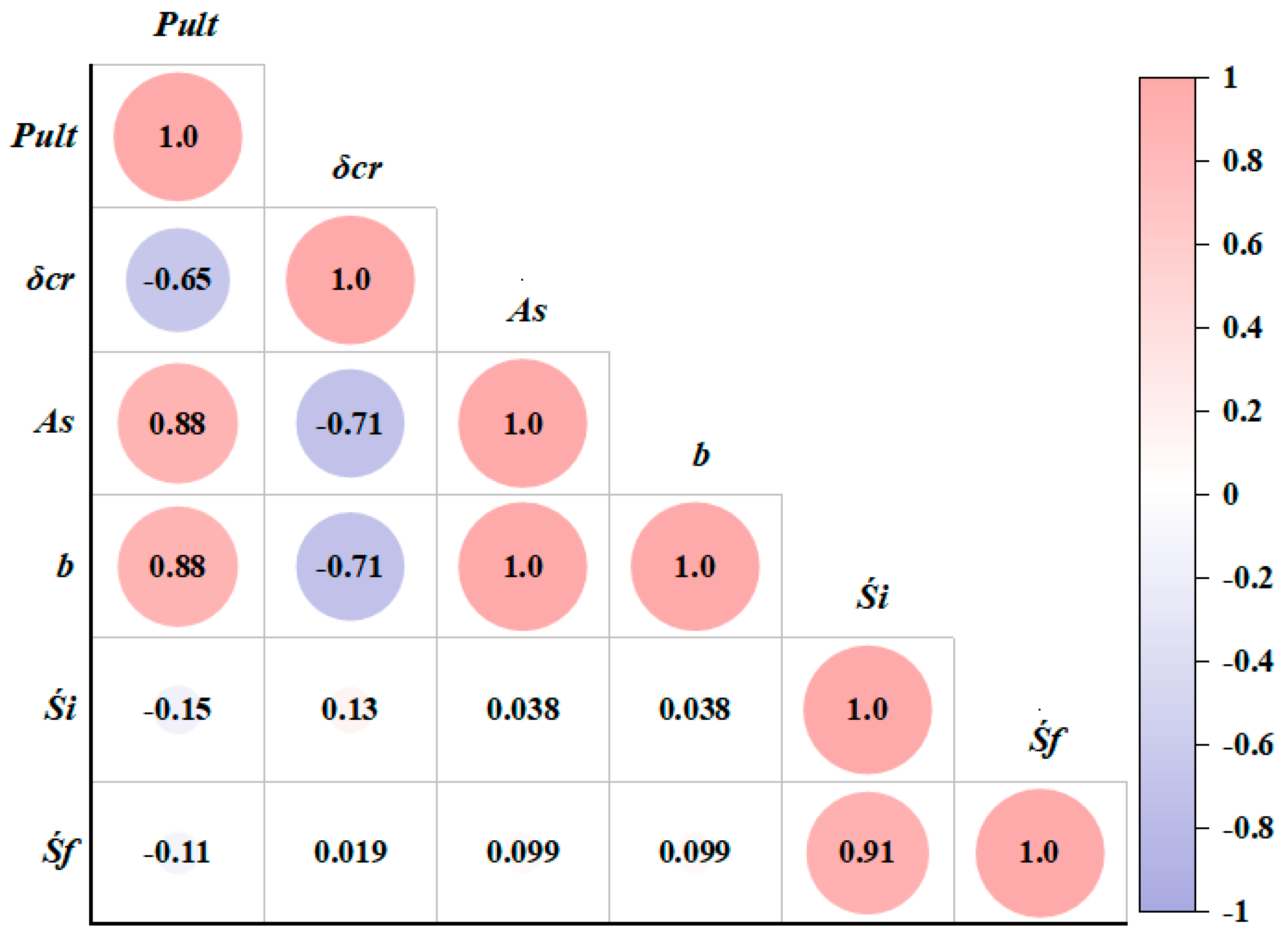
The choice of the input parameters in developing any model is critical for achieving accurate prediction skills. Therefore, including unfitting parameters in the modelling and resulting to the reduced performance accuracies will cause the high computational tasks [36,53]. Nevertheless, insufficient input parameters can lead to the reduced estimation accuracy. Thus, Pearson correlation was utilized in our work to decide on the most important input parameters for estimating the final strand slips of the HCU slabs subjected to flexural loading. Figure 9 shows the results of sensitivity analysis involving the potential input and output parameters. The analysis showed that the initial strand slip is the most sensitive parameter for predicting the final strand slip (Ś_f). All others input parameters demonstrate lower correlation coefficient values with the output parameters.

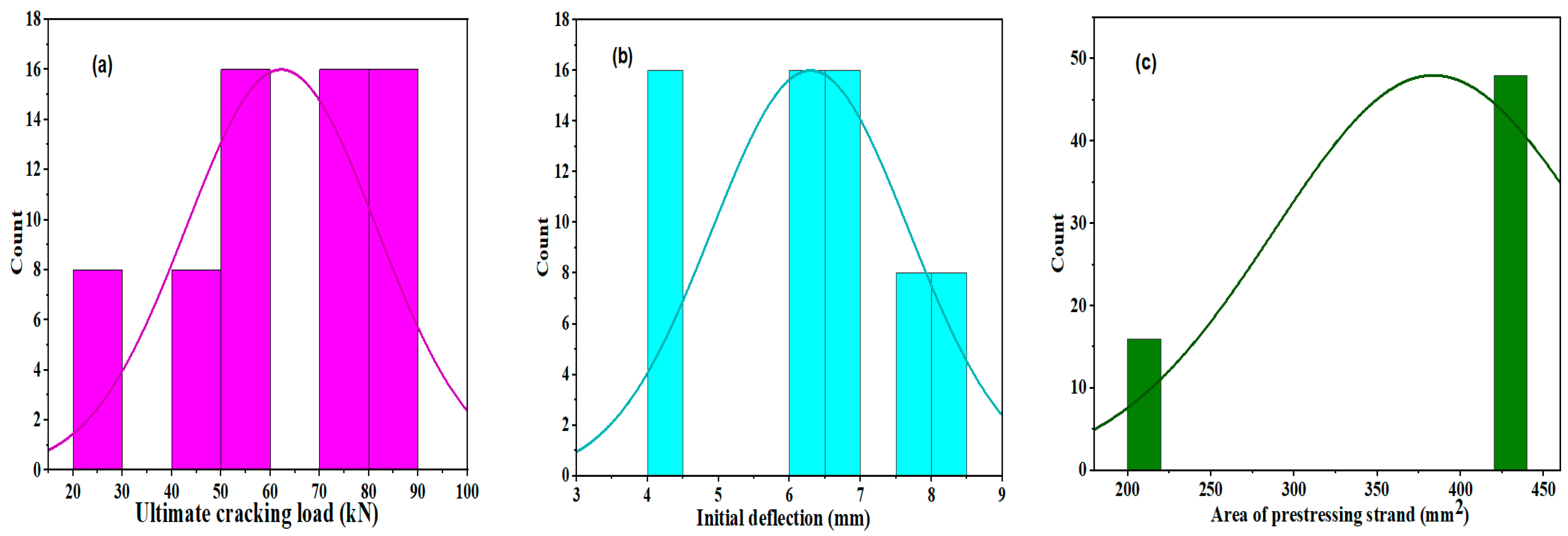
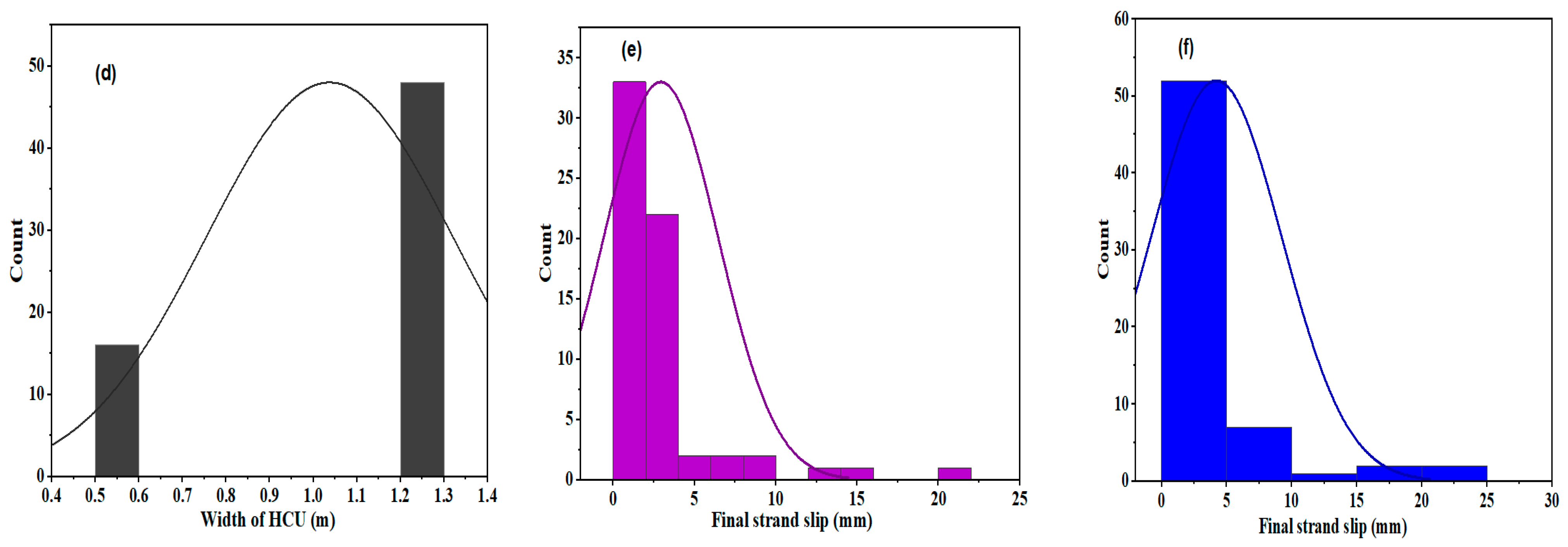
The frequency distributions of the dataset utilized to estimate the final strand slips of the HCU slabs under flexural loading are shown in Figure 10. The figures showed that potential datasets did not follow the normal distributions. The frequently used values of the ultimate cracking load ranged from 70 kN to 90 kN. Most of the initial crack deflections were between 6 and 7 mm, and the strand area and width of the HCU-WBs were used. The most frequently used initial and final strand slip values were between 0.1 and 5 mm.

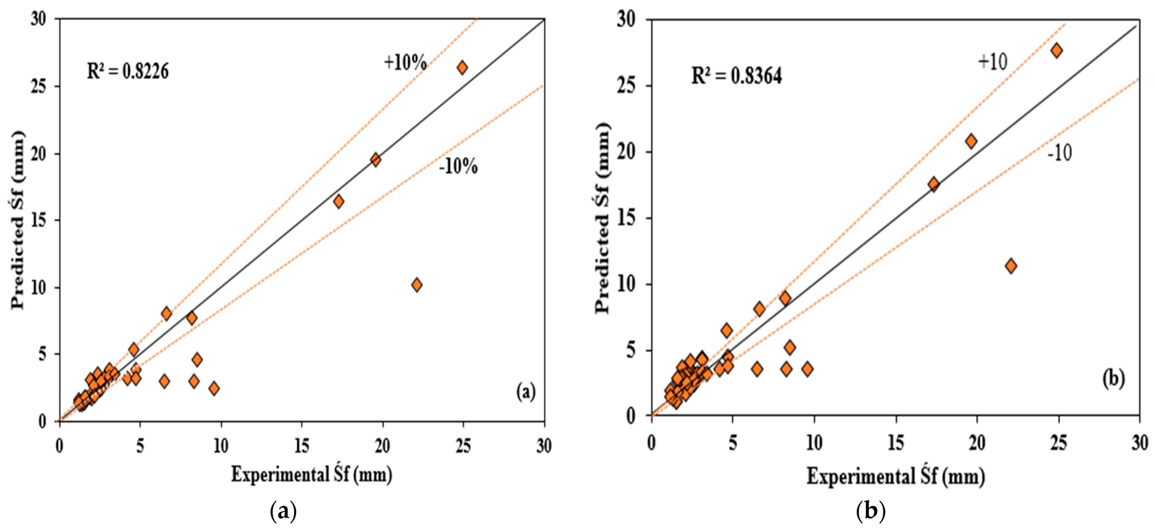
The MATLAB (2021a) toolbox (Machine learning) was used to develop the classical and hybrid models. The validation of the classical model was carried out using a 10-fold cross-validation technique [22,24]. The models used were the trained and tested dataset. The performances of the models were determined using the evaluation metrices and are summarized in

Table 7. Developed model performance result.

Models	Phase	R2	MAE	RMSE	MAPE	RI
SVM	Training	0.8226	0.0438	1.1237	4.379	1.5321
	Testing	0.9293	0.0236	0.0247	2.365	0.8043
MLR	Training	0.8364	0.0491	1.0903	4.908	2.0159
	Testing	0.8949	0.0361	0.3635	3.613	1.3375
IEPANN	Training	0.9168	0.0381	0.0826	3.802	1.3100
	Testing	0.9701	0.0138	0.0004	1.138	0.4651

. As shown in Table 7, all the developed models estimated the strand slips with high accuracies in the two modelling stages with the R² values > 0.8. Moreover, the IEPANN outperformed the other classical model in forecasting Śf in the precast HCUs with the R² values of 0.9168 in the training phase and 0.9701 in the attesting phase. The normalized RI values were used to assess the performances of both the classical and hybrid models because the other evaluation indicators might not effectively reflect the combined errors of the developed models. As can be observed, the hybrid IEPANN model performed best in the training and testing phases with the RI values of 1.31 and 0.4651.

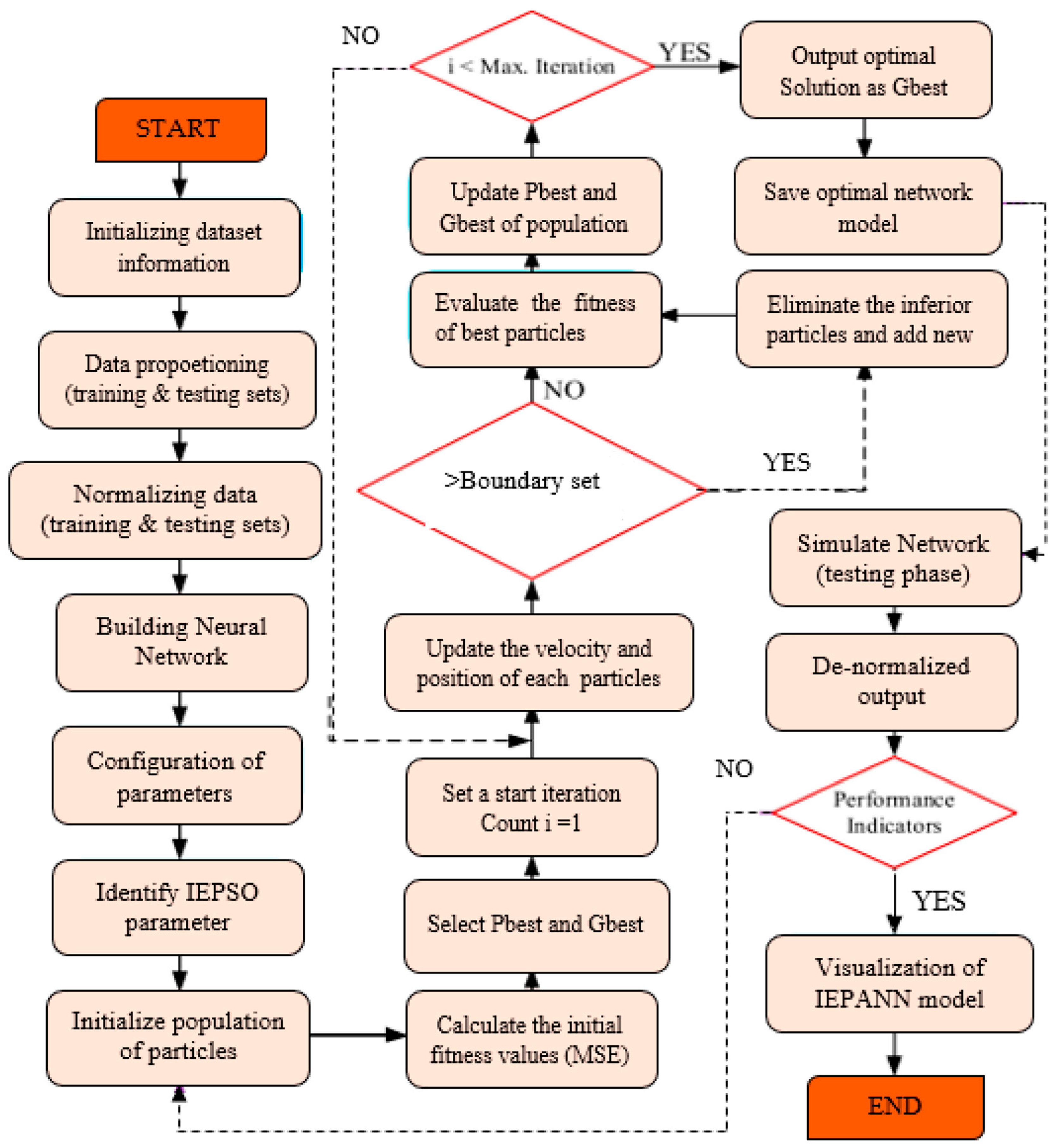
6.2. Classical Model

Figure 11 shows the scatters between the measured and predicted values in the training phase. The data points were converged along the fitting lines of the models, resulting in better goodness of fit. The dotted lines on both sides represent the confidence intervals of ±10%. Comparing the R² values of the single models as shown in Figure 11 and Figure 12, all the models predicted the strand slips with high accuracies, and the SVM outperformed the other single models with the R² values of 0.8226 in the training phase and 0.9293 in the testing phase. However, the R² value in the training phase of the MLR was higher than that of the SVM. The training dataset of the SVM model revealed higher RMSE and MAPE values than the MLR models. They are relatively high, translating large dispersions between the predicted and actual values. This result is attributed to the nonlinear behaviors of the dataset, which were unable to predict the strand slips with high accuracies using simple linear models. Generally, the prediction skills of the classical model in the testing phase were greater than those in the training phase, as shown in Figure 12.

6.3. IEPANN

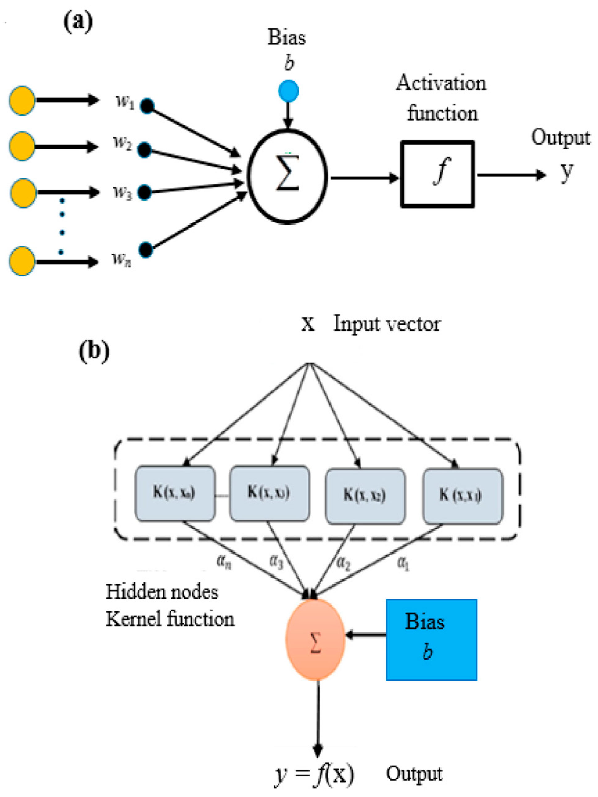
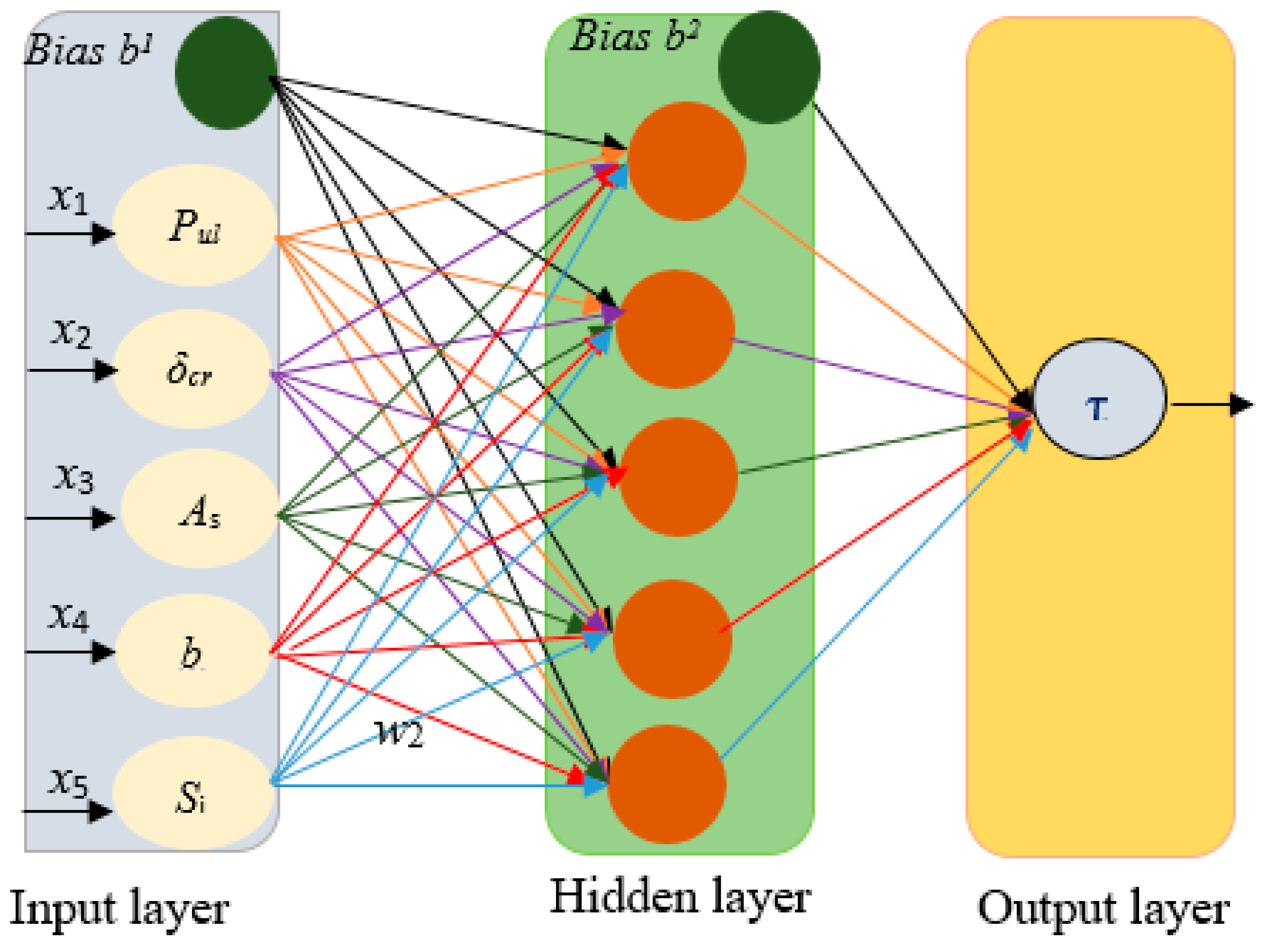
To develop the IEPANN model, this study implemented one hidden layer of the ANN, as recommended in some previous studies [47,48]. Therefore, a trial run with two to nine neurons achieved the optimal neuron number. The model was trained using Levenberg–Marquardt back-propagation techniques, with Purelin in the output layer and Tansig in the hidden layer. The general operating theory of the ANN model for estimating the Śf is expressed as

$$\tau =purelin\left\{b_x+{\displaystyle \sum _{j=1}^5\left[w_j\times Tansig(b_{hj}+{\displaystyle \sum _{i=1}^5{w}_{ij}{I}_j)}\right]}\right\}$$

(13)

where b_x and w_j are the bias in the output and the weight joining the jth neuron in the hidden and output, w_ij is the weight of the connection between the ith input parameter and the neuron in the hidden layer, b_hj is the bias in the jth neuron of the hidden neuron, and I_i is the input parameter i.

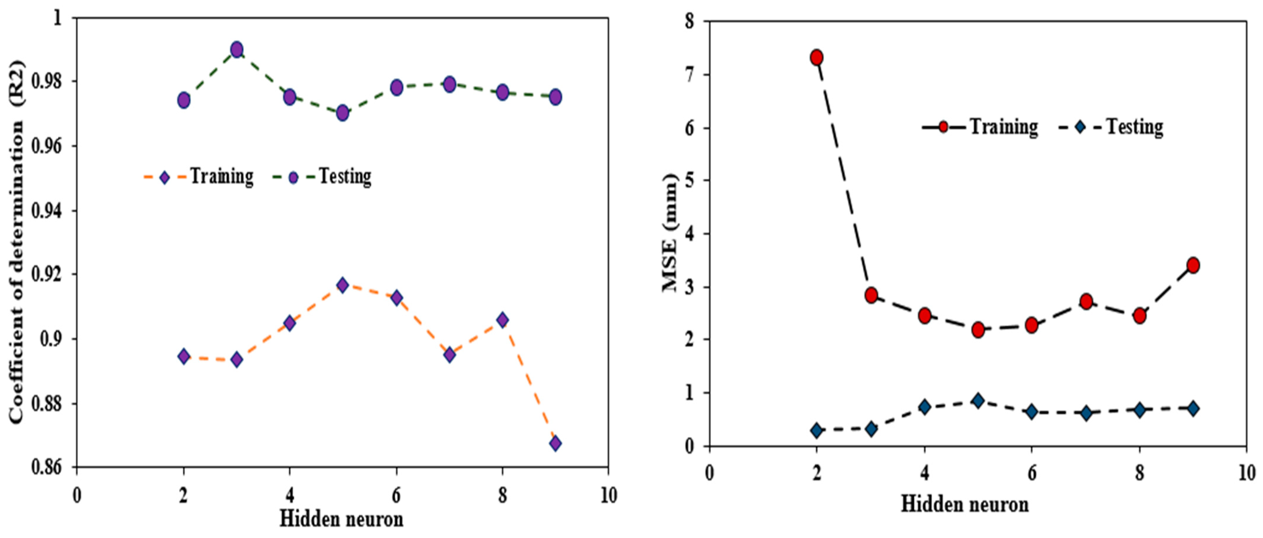
Figure 13 shows the performances of the IEPANN model. It can be observed that the IEPANN technique exhibiting five neurons in the hidden layer (5 $\times$ 5 × 1) outperformed the other single models with the R² values of 0.9168 in the training phase and 0.9701 in the testing phase, with the lowest MSE values of 0.0836 and 0.0299, respectively. The structure of the optimal IEPANN is shown in Figure 14.

Subsequently, the learning approach was to optimize the ANN weight and bias with the IEPSO. In this process, parameters such as population size, velocity coefficient, inertia weight, the local–global information sharing parameter, and stopping criteria were optimized in the ANN model. The coefficients of the velocities V₁ and V₂ are described according to [54], as given in Equation (14) below.

$$V_1=\lambda {\varphi }_1, V_2=\lambda {\varphi }_2, \lambda =\frac{2}{\phi -2\sqrt{{\varphi }^2-4\varphi }}, \varphi ={\varphi }_1+{\varphi }_2$$

(14)

The construction coefficient ϕ₁ = ϕ₂ − 2.05, the dumping ratio = 1, and w = 0.7280, with the upper bound velocity of −5 and the lower bound velocity of 5, respectively. Equation (10) was used to determine c₃. Moreover, different swarm sizes were explored in this study to obtain the optimal size. Swarm sizes of 100, 150, 200, …., 300 were adopted. The maximum iteration of the IEPSO approach was regarded as its criterion for stopping. The sensitivity study showed that the MSE value remained constant after 150 iterations, which was thought to be the optimal iteration. The right swarm size was selected based on these iterations, considering the R² and MSE values. Therefore, the IEPANN model having 120 populations exhibited the highest R² and lowest MSE values in the two modelling phases, and thus considered the optimal model.

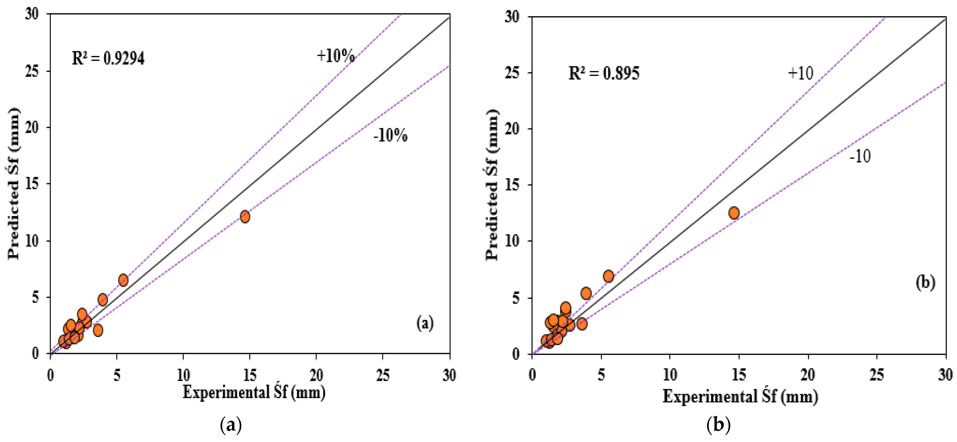
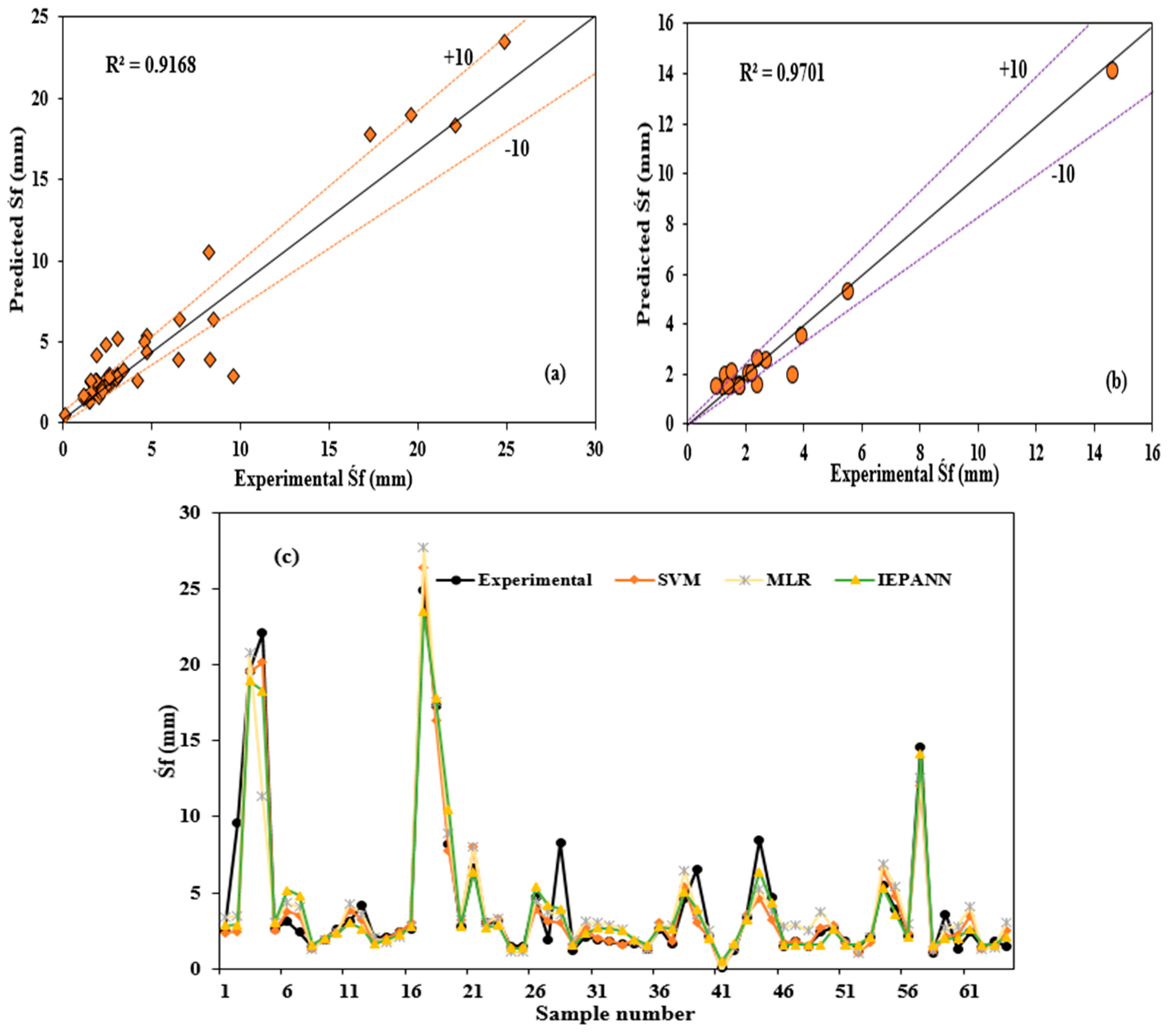
Figure 15 presents the scatters between the experimental and predicted results obtained from the IEPANN model in the modelling phases. As shown in Figure 15, good agreements between the measured and predicted values were achieved, and data points were close to the fitted lines. The prediction skills of the IEPANN model in the testing phase were higher than those in the training phase. This is similar to the results obtained in the two single models, which is attributed to the dataset involved in the modelling in the testing phase. Moreover, the overall performances of all developed models were provided for comparisons, as depicted in Figure 15c, which defined the relationships between the observed and predicted values for individual models. The predicted data points were close to the actual data, indicating the effectiveness and accuracy of the developed model, particularly the IEPANN model, for predicting the final prestressing strand slips considering the nonlinearity relations between the input parameters and strand slips. In the related study by Alhassan et al. [13], which determine the optimal prediction of the transfer length (TL) of prestressing strand based on the ANN model, the results showed the ANN predicted the TL with high prediction skills with all R² values greater than 0.9.

To provide an explicit equation for the final strand slip (Śf), Equation (15) is modified by computing and substituting the optimum weight and bias of the trained IEPANN model.

$$\tau =24.9(0.320y_1-0.540y_2-0.698y_3-0.598y_4+2.622y_5+2.127)+0.1$$

(15)

where y₁, y₂, …, y₅ are determined using the input variables as:

$$y_1=Tansig(-0.496P_{ult}-0.507{\delta }_{cr}-0.610A_s-3.951b-0.279{\zeta }_i-0.237)$$

(16)

$$y_2=Tansig(-0.914P_{ult}-2.478{\delta }_{cr}-1.282A_s+1.127b-2.230{\zeta }_i-0.519)$$

(17)

$$y_3=Tansig(0.861P_{ult}+4.799{\delta }_{cr}-1.216A_s-0.807b-0.302{\zeta }_i-04.245)$$

(18)

$$y_4=Tansig(3.166P_{ult}+1.856{\delta }_{cr}-0.826A_s-1.427b-0.974{\zeta }_i+1.363)$$

(19)

$$y_5=Tansig(-1.557P_{ult}+1.852{\delta }_{cr}-0.310A_s+0.810b+0.119{\zeta }_i-3.379)$$

(20)

In addition, Equation (21) was used to determine the activation function as

$$Tansig(x)=\frac{2}{1+e^{-2x}}+1$$

(21)

From Equations (16)–(20), it is clear that all the input variables were multiplied by the weight, and the bias of the optimum IEPANN model was added to the sum. Following the determination of the nonlinear activation function, Equation (15) was used to analyse the prestressing strand slips.

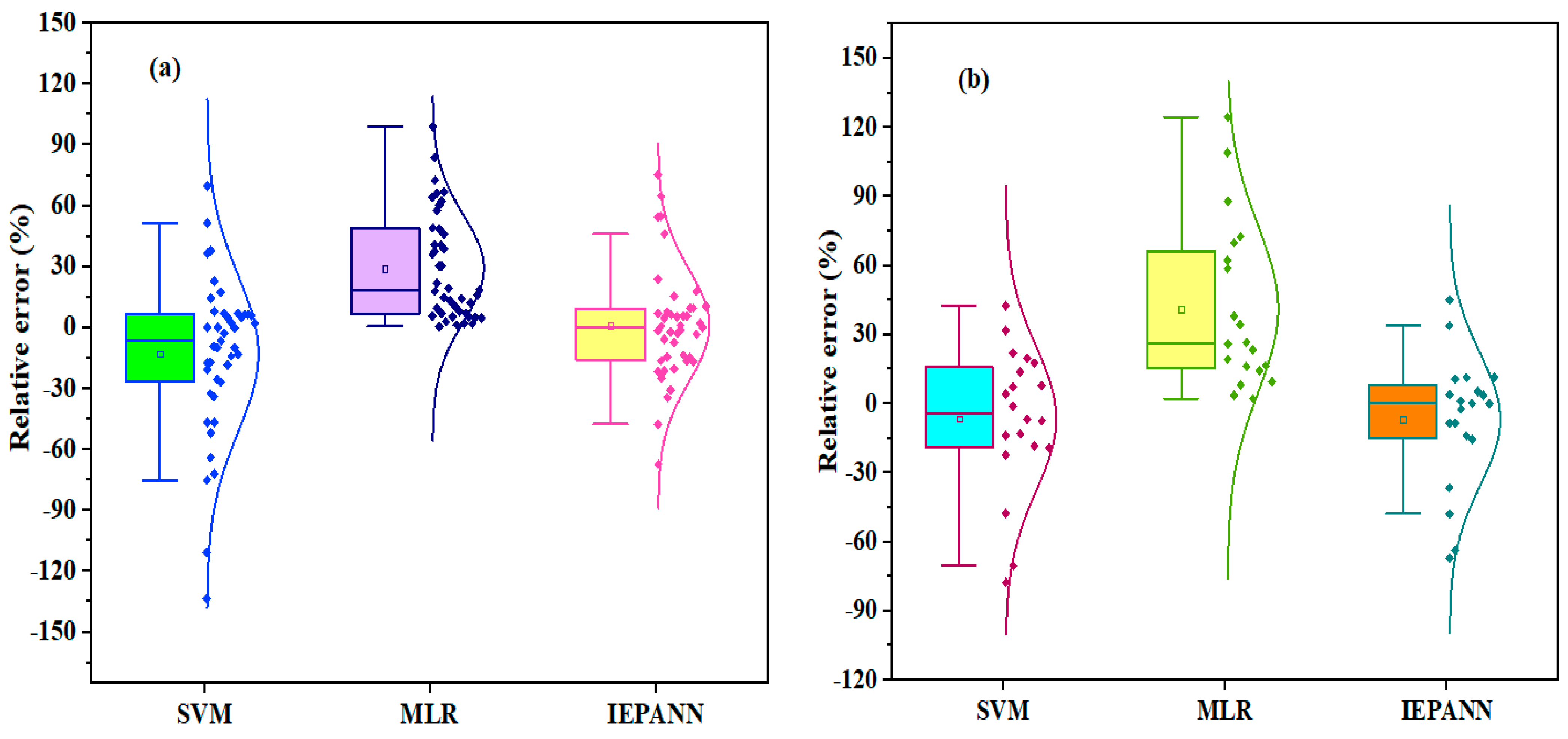
The relative error distributions obtained from individual models were used to evaluate the accuracy of the ML. Boxplot was used to compare the relative error distributions for individual models in the training and testing phases, as shown in Figure 16. From Figure 16a, it can be noted that the IEPANN demonstrated the highest accuracy with the lowest maximum and minimum relative error distributions in estimating the final strand slips in the training stage, with the first quartile (Q1) and third quartile (Q3) values of −8.6% and −15%. Secondly, the SVM was the second model with the lowest relative error distributions, with the minimum relative error distribution of 7.5% and the maximum relative error distribution of −22.3%.

Generally, the relative error distributions exhibited by all the MLs were slighly higher in the training phase compared to those in the testing stage, as depicted in Figure 16a. Similarly, from Figure 16b, the lowest error distributions were obtained in the IEPANN and SVM models in the testing phase. The minimum and maximum error distributions in Q1 and Q3 were −14.2% and 8%, respectively. Thes results were consistent with the highest performances of the IEPANN model in the scatter curves for the two modeling stages, compared to other models (MLR, SVM).

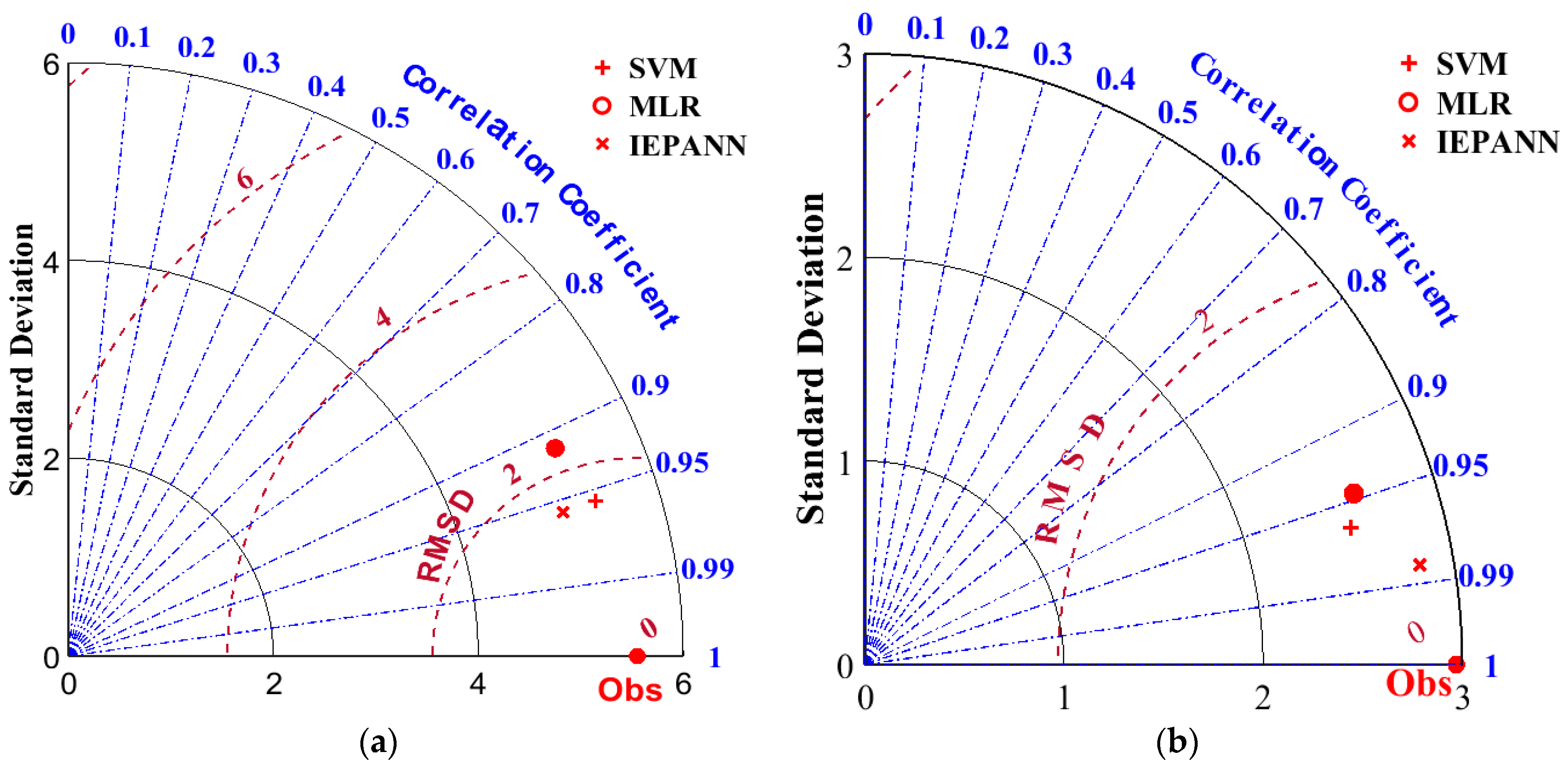
Furthermore, the performances of the ML model in the two modeling phases were also checked using the Taylor diagram, as shown in Figure 17. The Taylor diagram is a compressive approach for comparing model performances using three statistical parameters: RMSE, R² and SD. The correlation between the measured and predicted values was specified by the azimuthal point, i.e., the location where the measured and predicted fields were directly correlated with the RMSE values. The RMSE values decreased with the increases in correlations. As a result, the radial distance measured from the origin increased with an increasing trend of the standard deviation [55]. The perfect model is achieved by reference point with R² = 1 [56]. However, if the predicted SD is greater than that of the observed data, overestimation may occur, or vice versa. Therefore, it is necessary to use a standard deviation approach to obtain the SD of the observed data.

From Figure 17a,b, the hybridized IEPANN models demonstrated higher performances in estimating the strand slips in the precast prestressed HCUs with RMSE, R, and SD closer to the actual data in both training and testing phases. The scatter plots showed that the hybridized IEPANN outperformed all other models in terms of all evaluation matrices. The standard deviations of all the models were lower than those of the actual data, proving that models were not affected by overestimation.

7. Conclusions

The additional strand slips in prestressed concrete hollow-core slabs subjected to three-point bending were investigated through load tests on five full-scale specimens. Two groups of HCUs characterized by wide and narrow widths were experimentally tested with or without a topping slab, and a wide specimen was tested with restrain mechanism at its ends. Moreover, single (SVM, MLR) and hybrid (IEPANN) machine learning algorithms were employed to estimate the final strand slips after the bending tests. Sensitivity analysis using Person correlation was applied to explore optimal input parameters, which involved the ultimate deflection, initial deflection, strand area, width of HBCUs, and initial strand slip. Five performance criteria, including R², RSME, MAE, MAPE, and RI, were utilized to assess the performances of the developed ML algorithms. Finally, a Box plot and Taylor diagram were used to compare the model performances visually for predicting the final strand slips of the prestressed hollow-core slabs. The conclusions outlined in this study are stated below:

(1)

The initial strands slip values at the ends of HCUs in most of the strands ranged between 2 and 3 mm. However, an initial strand slip of 21 mm was obtained in one of the strands of the HCU-WB specimen at the south end with a peak final slip of 24.9 mm, indicating that the prestressing strands with relatively higher initial strand slips may result in larger additional slips during flexural loading. Some strands revealed no additional strand slips after testing.

(2)

Non-composite (HCU-WB and HCU-NB) specimens sustained web shear failure, while composite (HCU-WT, HCU-WTR, and HCU-NT) specimens showed vertical separations between the HCUs and topping slab. The restraining mechanism and cast-in-place topping slab influenced the rate of additional strand slips.

(3)

The feature selection analysis revealed that the initial strand slip was the most relevant parameter for predicting the final strand slip among the input parameters. Both single and hybrid ML models estimated the final strand slips of HCUs with high accuracies in the training and testing phases. Moreover, the hybridized IEPANN model showed the highest prediction skills with the R² values of 0.9168 and 0.970 in the training and testing phases, respectively, demonstrating the efficacy of the IEPANN compared to the nonlinear predictive model.

(4)

The addition strand slips in precast prestressed hollow-core slabs subjected to high-intensity loads were evaluated, as in the cases of car parks and bridges. The prediction skills could prevent the need for conducting high-cost experiments and save time. Additionally, recent and advanced ML algorithms, such as hybrid and ensemble models and numerical expressions, are recommended for the estimation of the additional strand slips. The evaluation could serve as a guide for engineering practice.

(5)

The research is limited to a small dataset obtained from the experimental program to predict the final strand slips of the precast prestressed concrete hollow-core slabs. Modeling tasks required a large database to achieve the highest accurate and reliable prediction model. On the other hand, the small database could also give reasonable prediction accuracy.

References

1. Chen, L.; Han, C.; Xu, Q.; Wang, Y.C.; Li, M.; Leng, Y. Postfire performance of prestressed concrete hollow-core floor systems with edge beams. J. Struct. Eng. 2020, 146, 4020262. [Google Scholar] [CrossRef]
2. Hegger, J.; Roggendorf, T.; Kerkeni, N. Shear capacity of prestressed hollow core slabs in slim floor constructions. Eng. Struct. 2009, 31, 551–559. [Google Scholar] [CrossRef]
3. Wang, Z.; Wang, M.; Xu, Q.; Harries, K.A.; Li, X.; Gao, R. Experimental research on prestressed concrete hollow-core slabs strengthened with externally bonded bamboo laminates. Eng. Struct. 2021, 244, 112786. [Google Scholar] [CrossRef]
4. Zhang, H.; Huang, W.; Liu, B.; Han, C.; Li, Q.; Chen, C. Flexural behavior of precast concrete hollow-core slabs with high-strength tendons. J. Build. Eng. 2022, 59, 105050. [Google Scholar] [CrossRef]
5. Walraven, J.C.; Mercx, W.P.M. The bearing capacity for prestressed hollow core slabs. Heron 1983, 28, 1–46. [Google Scholar]
6. Anderson, A.R.; Anderson, R.G. An assurance criterion for flexural bond pretensioned hollow core units. ACI J. 1976, 73, 457–464. [Google Scholar]
7. Haruna, S.İ. Flexural Behavior of Precast Prestressed Concrete Hollow Core Slabs with Cast-in-Place Concrete Topping. Master’s Thesis, Atilim University, Ankara, Turkey, 2014. [Google Scholar]
8. ACI 318-83; Building Code Requirements for Reinforced Concrete. American Concrete Institute: Detroit, MI, USA, 1983.
9. Marti-Vargas, J.R. Analysis and prediction of transfer length in pretensioned, prestressed concrete members. ACI Struct. J. 2015, 112, 237–239. [Google Scholar]
10. Oh, B.H.; Lim, S.N.; Lee, M.K.; Yoo, S.W. Analysis and prediction of transfer length in pretensioned, prestressed concrete members. ACI Struct. J. 2014, 111, 549. [Google Scholar] [CrossRef]
11. Joo, H.-E.; Han, S.-J.; Kim, K.S. Analytical model for shear strength of prestressed hollow-core slabs reinforced with core-filling concrete. J. Build. Eng. 2021, 42, 102819. [Google Scholar] [CrossRef]
12. Dang, C.N.; Floyd, R.W.; Hale, W.M.; Martí-Vargas, J.R. Measured transfer lengths of 0.7 in (17.8 mm) strands for pretensioned beams. ACI Struct. J. 2016, 113, 85–94. [Google Scholar]
13. Alhassan, M.A.; Ababneh, A.N.; Betoush, N.A. Optimum prediction of the transfer length of strands based on artificial neural networks. Procedia Manuf. 2020, 44, 505–512. [Google Scholar] [CrossRef]
14. ACI 318-08; Committee Building Code Requirements for Structural Concrete and Commentary. American Concrete Institute: Detroit, MI, USA, 2008.
15. Oh, B.H.; Kim, E.S. Realistic evaluation of transfer lengths in pretensioned, prestressed concrete members. ACI Struct. J. 2000, 97, 821–830. [Google Scholar]
16. Russell, B.W.; Burns, N.H. Design Guidelines for Transfer, Development and Debonding of Large Diameter Seven Wire Strands in Pretensioned Concrete Girders; Research Report 1210-5F; Center for Transportation Research, The University of Texas: Austin, TX, USA, 1993. [Google Scholar]
17. Martí-Vargas, J.R.; Serna, P.; Navarro-Gregori, J.; Pallarés, L. Bond of 13 mm prestressing steel strands in pretensioned concrete members. Eng. Struct. 2012, 41, 403–412. [Google Scholar] [CrossRef]
18. BS EN 1992-1-1; Eurocode 2: Design of Concrete Structures—Part 1-1: General Rules and Rules for Buildings. British Standards Institution: London, UK, 2004.
19. Fan, W.; Chen, Y.; Li, J.; Sun, Y.; Feng, J.; Hassanin, H.; Sareh, P. Machine learning applied to the design and inspection of reinforced concrete bridges: Resilient methods and emerging applications. Structures 2021, 33, 3954–3963. [Google Scholar] [CrossRef]
20. Dang, H.V.; Trestian, R.; Thanh, B.-T.; Nguyen, H.X. Probabilistic method for time-varying reliability analysis of structure via variational bayesian neural network. Structures 2021, 34, 3703–3715. [Google Scholar] [CrossRef]
21. Haruna, S.I.; Malami, S.I.; Adamu, M.; Usman, A.G.; Farouk, A.I.B.; Ali, S.I.A.; Abba, S.I. Compressive strength of self-compacting concrete modified with rice husk ash and calcium carbide waste modeling: A feasibility of emerging emotional intelligent model (EANN) versus traditional FFNN. Arab. J. Sci. Eng. 2021, 46, 11207–11222. [Google Scholar] [CrossRef]
22. Haruna, S.I.; Zhu, H.; Jiang, W.; Shao, J. Evaluation of impact resistance properties of polyurethane-based polymer concrete for the repair of runway subjected to repeated drop-weight impact test. Constr. Build. Mater. 2021, 309, 125152. [Google Scholar] [CrossRef]
23. Adamu, M.; Haruna, S.I.; Malami, S.I.; Ibrahim, M.N.; Abba, S.I.; Ibrahim, Y.E. Prediction of compressive strength of concrete incorporated with jujube seed as partial replacement of coarse aggregate: A feasibility of Hammerstein–Wiener model versus support vector machine. Model. Earth Syst. Environ. 2021, 8, 3435–3445. [Google Scholar] [CrossRef]
24. Farouk, A.I.B.; Zhu, J. Prediction of interface bond strength between ultra-high-performance concrete (UHPC) and normal strength concrete (NSC) using a machine learning approach. Arab. J. Sci. Eng. 2022, 47, 5365–5375. [Google Scholar] [CrossRef]
25. Rehman, K.U.; Çolak, A.B.; Shatanawi, W. Artificial neural networking (ANN) model for drag coefficient optimization for various obstacles. Mathematics 2022, 10, 2450. [Google Scholar] [CrossRef]
26. Almustafa, K.M.; Sharma, A.K.; Bhardwaj, S. STARC: Deep learning Algorithms’ modelling for STructured analysis of retina classification. Biomed. Signal Process. Control 2023, 80, 104357. [Google Scholar] [CrossRef]
27. Nourani, V.; Asghari, P.; Sharghi, E. Artificial intelligence-based ensemble modeling of wastewater treatment plant using jittered data. J. Clean. Prod. 2021, 291, 125772. [Google Scholar] [CrossRef]
28. Chou, J.-S.; Nguyen, N.-M. Metaheuristics-optimized ensemble system for predicting mechanical strength of reinforced concrete materials. Struct. Control Health Monit. 2021, 28, e2706. [Google Scholar] [CrossRef]
29. Liang, M.; Chang, Z.; Wan, Z.; Gan, Y.; Schlangen, E.; Šavija, B. Interpretable Ensemble-Machine-Learning models for predicting creep behavior of concrete. Cem. Concr. Compos. 2022, 125, 104295. [Google Scholar] [CrossRef]
30. Zhang, S.-Y.; Chen, S.-Z.; Jiang, X.; Han, W.-S. Data-driven prediction of FRP strengthened reinforced concrete beam capacity based on interpretable ensemble learning algorithms. Structures 2022, 43, 860–877. [Google Scholar] [CrossRef]
31. Pan, L.X.; Lehký, D.; Novák, D.; Cao, M. Sensitivity analysis for parameters of prestressed concrete bridge using neural network ensemble. In Proceedings of the 24th International Conference on Engineering Mechanics 2018, Svratka, Czech Republic, 14–17 May 2018; pp. 637–640. [Google Scholar] [CrossRef] [Green Version]
32. Fati, S.M.; Senan, E.M.; El Hakim, N. Deep and hybrid learning technique for early detection of tuberculosis based on X-ray images using feature fusion. Appl. Sci. 2022, 12, 7092. [Google Scholar] [CrossRef]
33. Fati, S.M.; Senan, E.M.; Azar, A.T. Hybrid and deep learning approach for early diagnosis of lower gastrointestinal diseases. Sensors 2022, 22, 4079. [Google Scholar] [CrossRef] [PubMed]
34. Doğan, G.; Arslan, M.H. Determination of punching shear capacity of concrete slabs reinforced with FRP bars using machine learning. Arab. J. Sci. Eng. 2022, 47, 13111–13137. [Google Scholar] [CrossRef]
35. Sharghi, E.; Nourani, V.; Zhang, Y.; Ghaneei, P. Conjunction of cluster ensemble-model ensemble techniques for spatiotemporal assessment of groundwater depletion in semi-arid plains. J. Hydrol. 2022, 610, 127984. [Google Scholar] [CrossRef]
36. Ali, N.M.; Farouk, A.I.B.; Haruna, S.I.; Alanazi, H.; Adamu, M.; Ibrahim, Y.E. Feature selection approach for failure mode detection of reinforced concrete bridge columns. Case Stud. Constr. Mater. 2022, 17, e01383. [Google Scholar] [CrossRef]
37. Arslan, M.H.; Özkılıç, Y.O.; Arslan, H.D.; Şahin, Ö.S. Experimental and numerical investigation of the structural, thermal and acoustic performance of reinforced concrete slabs with balls for a cleaner environment. Int. J. Civ. Eng. 2023, 21, 789–804. [Google Scholar] [CrossRef]
38. Kankeri, P.; Prakash, S.S.; Pachalla, S.K.S. Experimental and numerical studies on efficiency of hybrid overlay and near surface mounted FRP strengthening of pre-cracked hollow core slabs. Structures 2018, 15, 1–12. [Google Scholar] [CrossRef]
39. De Souza, J.R.; Araujo, D.L. Shear capacity of prestressed hollow core slabs in flexible support using computational modelling. Eng. Struct. 2022, 260, 114243. [Google Scholar] [CrossRef]
40. Abdelatif, A.O.; Owen, J.S.; Hussein, M.F.M. Modelling the prestress transfer in pre-tensioned concrete elements. Finite Elem. Anal. Des. 2015, 94, 47–63. [Google Scholar] [CrossRef]
41. Ghaffari, A.; Abdollahi, H.; Khoshayand, M.; Bozchalooi, I.; Dadgar, A.; Rafiee-Tehrani, M. Performance comparison of neural network training algorithms in modeling of bimodal drug delivery. Int. J. Pharm. 2006, 327, 126–138. [Google Scholar] [CrossRef] [PubMed]
42. Farouk, A.I.B.; Zhu, J.; Ding, J.; Haruna, S.I. Prediction and uncertainty quantification of ultimate bond strength between UHPC and reinforcing steel bar using a hybrid machine learning approach. Constr. Build. Mater. 2022, 345, 128360. [Google Scholar] [CrossRef]
43. Nourani, V.; Elkiran, G.; Abba, S.I. Wastewater treatment plant performance analysis using artificial intelligence—An ensemble approach. Water Sci. Technol. 2018, 78, 2064–2076. [Google Scholar] [CrossRef] [Green Version]
44. Wang, W.; Xu, D.; Chau, K.; Chen, S. Improved annual rainfall-runoff forecasting using PSO–SVM model based on EEMD. J. Hydroinform. 2013, 15, 1377–1390. [Google Scholar] [CrossRef]
45. Pablo, M.; Emad, M.; Osama, M.; Yasser, M. Comparative study of data mining models for prediction of bridge future conditions. J. Perform. Constr. Facil. 2020, 34, 4019108. [Google Scholar]
46. Lv, X.; Wang, Y.; Deng, J.; Zhang, G.; Zhang, L. Improved particle swarm optimization algorithm based on last-eliminated principle and enhanced information sharing. Comput. Intell. Neurosci. 2018, 2018, 5025672. [Google Scholar] [CrossRef] [Green Version]
47. Keshtegar, B.; Bagheri, M.; Yaseen, Z.M. Shear strength of steel fiber-unconfined reinforced concrete beam simulation: Application of novel intelligent model. Compos. Struct. 2019, 212, 230–242. [Google Scholar] [CrossRef]
48. Onyari, E.K.; Ikotun, B.D. Prediction of compressive and flexural strengths of a modified zeolite additive mortar using artificial neural network. Constr. Build. Mater. 2018, 187, 1232–1241. [Google Scholar] [CrossRef]
49. Zang, H.; Cheng, L.; Ding, T.; Cheung, K.W.; Wang, M.; Wei, Z.; Sun, G. Application of functional deep belief network for estimating daily global solar radiation: A case study in China. Energy 2020, 191, 116502. [Google Scholar] [CrossRef]
50. Brooks, M.D.; Gerstle, K.H.; Logan, D.R. Effect of initial strand slip on the strength of hollow-core slabs. PCI J. 1988, 33, 90–111. [Google Scholar] [CrossRef]
51. Palmer, K.D.; Schultz, A.E. Experimental investigation of the web-shear strength of deep hollow-core units. PCI J. 2011, 56, 83–104. [Google Scholar] [CrossRef]
52. Guyon, Y. Béton Précontraint: Constructions Hyperstatiques; Eyrolles: Paris, France, 1958. [Google Scholar]
53. Ahmed, A.A.; Pradhan, B. Vehicular traffic noise prediction and propagation modelling using neural networks and geospatial information system. Environ. Monit. Assess. 2019, 191, 190. [Google Scholar] [CrossRef]
54. Poli, R.; Kennedy, J.; Blackwell, T. Particle swarm optimization. Swarm Intell. 2007, 1, 33–57. [Google Scholar] [CrossRef]
55. Taylor, K.E. Summarizing multiple aspects of model performance in a single diagram. J. Geophys. Res. 2001, 106, 7183–7192. [Google Scholar] [CrossRef]
56. Yaseen, Z.M.; Deo, R.C.; Hilal, A.; Abd, A.M.; Bueno, L.C.; Salcedo-Sanz, S.; Nehdi, M.L. Predicting compressive strength of lightweight foamed concrete using extreme learning machine model. Adv. Eng. Softw. 2018, 115, 112–125. [Google Scholar] [CrossRef]
Figure 1. Transfer of prestress in pretensioned concrete.
Buildings 13 02013 g001
Figure 2. Geometric details of the HCU Specimens.
Buildings 13 02013 g002
Figure 3. Instrumentation for additional strand slips.
Buildings 13 02013 g003
Figure 4. Architecture of: (a) ANN model, (b) SVM model.
Buildings 13 02013 g004
Figure 5. Schematic flowchart of the IEPANN model.
Buildings 13 02013 g005
Figure 6. Failure modes of: (a) HCU-WB, (b) HCU-NB, (c) HCU-WT, and (d) HCU-NT.
Buildings 13 02013 g006
Figure 7. Additional strand slip for (a) HCU-WB, (b) HCU-WT, (c) HCU-WTR, (d) HCU-NB, and (e) HCU-NT.
Buildings 13 02013 g007
Figure 8. Strand slip vs. midspan deflection curves for: (a) HCU-WB, (b) HCU-WT, (c) HCU-WTR, (d) HCU-NB, and (e) HCU-NT.
Buildings 13 02013 g008aBuildings 13 02013 g008b
Figure 9. Sensitivity analysis results using the Pearson correlation matrix.
Buildings 13 02013 g009
Figure 10. Distribution curves of the experimental dataset. (a) Ultimate clacking load (kN); (b) Initial deflection (mm); (c) Area of prestressing strand (mm2); (d) Width of HCU (m); (e) Final strand slip (mm); (f) Final strand slip (mm).
Buildings 13 02013 g010aBuildings 13 02013 g010b
Figure 11. Scatters for the classical model between the predicted and experimental strand slips in the training phase: (a) SVM, (b) MLR.
Buildings 13 02013 g011
Figure 12. Scatters for the classical model between the predicted and experimental strand slips in the testing phase: (a) SVM, (b) MLR.
Buildings 13 02013 g012
Figure 13. Effects on the number of hidden neurons in the IEPANN model.
Buildings 13 02013 g013
Figure 14. The structure of the optimized IEPANN model.
Buildings 13 02013 g014
Figure 15. Scatters between the measured and predicted strand slips for the IEPANN model in: (a) training phase, (b) testing phase, (c) all developed models for overall datasets.
Buildings 13 02013 g015
Figure 16. Relative error distributions for the developed model using Boxplot in: (a) training and (b) testing stages.
Buildings 13 02013 g016
Figure 17. Comparisons of the performances of the model using Taylor diagram: (a) training phase, (b) testing phase.
Buildings 13 02013 g017