Article

Optimal Tuned Inerter Dampers for Vibration Control Performance of Adjacent Building Structures

1
School of Civil Engineering, Anhui Jianzhu University, Hefei 230601, China
2
Key Laboratory of Intelligent Underground Detection Technology, Anhui Jianzhu University, Hefei 230601, China
*
Author to whom correspondence should be addressed.
Buildings 2023, 13(7), 1803; https://doi.org/10.3390/buildings13071803
Submission received: 27 June 2023 / Revised: 8 July 2023 / Accepted: 13 July 2023 / Published: 15 July 2023
(This article belongs to the Special Issue Structural Vibration Control Research)

Abstract

:
Under the effect of strong earthquakes, collisions or excessive inter-story displacements may occur between adjacent building structures to the extent that the building structure is damaged. The traditional seismic measures for these structures can no longer meet the needs in practical engineering. In this paper, we propose the application of parallel and serial TID-based control systems in adjacent buildings as an example of a single-story adjacent building, and use it to form a new adjacent building seismic reduction structure. In this paper, the dynamic characteristics and design parameter optimization of the vibration control system are investigated by means of the Monte Carlo pattern search method and H2 norm theory. The results show that the introduction of serial and parallel TID in adjacent building structures can effectively improve the seismic resistance of adjacent buildings. The problem of vibration amplification caused by resonance is obviously improved, which is especially evident in the adjacent building structure vibration control system based on parallel TID. The vibration control system of adjacent building structures based on parallel TID is more robust. When optimizing the right building, the damping requirement of the TID decreases for the vibration control system based on parallel TID as the adjacent building mass ratio increases, while the damping requirement of the TID increases for the vibration control system based on serial TID. In both vibration control systems, the difference in the optimal inertial mass ratio is small. In practice, a moderate increase in the difference between adjacent building masses can have a positive effect on the vibration control performance of the systems. The main contribution of this paper is to fill the research gap in parallel and serial TID applications for adjacent building vibration reduction.

1. Introduction

In the past, some areas were extremely vulnerable to disasters due to poor building quality, resulting in serious personal casualties and property damage. Therefore, modern construction practices no longer simply pursue quantity, but pay more attention to quality and sustainability. Especially in areas where earthquakes are frequent or that have had disasters, people are more concerned about the seismic performance of buildings. A scientific approach to seismic design to ensure that buildings can withstand the forces of earthquakes and ensure the safety of people’s lives in the event of an earthquake is a research topic that has received widespread concern. Therefore, people have started to consider attaching control devices to the structures to suppress the seismic response of the structure, and this method is called the structural control technique.
For example, dampers such as the friction damper [1], the tuned liquid column damper (TLCD) [2,3] and viscous damper [4,5] are used in vibration control devices. Negative-stiffness systems are usually more efficient than conventional seismic isolation systems due to their ability to significantly reduce the vibration amplitude of the structure, while eliminating the inertial seismic loads to which the structure is subjected [6]. By introducing a new shape memory alloy into the negative-stiffness shock absorber, the device was able to effectively reduce the internal force response and displacement response of a bridge structural system [7]. A negative-stiffness amplifying damper can effectively reduce the interstory displacement and decrease the acceleration response of the structure [8]. In recent years, the KDamper has been proposed as a new passive vibration reduction concept. The KDamper is a device that significantly reduces the relative displacement of the base and can be implemented as a “rigid seismic absorption base”, while overcoming the shortcomings of conventional base isolation systems [9]. The optimized KDamper can effectively reduce the absolute acceleration response and displacement of a bridge. For spatially varying ground motions, the control effect of KDamper is very little affected [10].
In conclusion, tuned mass dampers (TMDs) are widely accepted as passive control devices. Under specific seismic motions, the use of TMDs can effectively reduce the hysteresis energy dissipation required for critical stories in the range of 1.8 to 2.8 s [11]. A TMD was also used to control the torsional response of a suspension bridge, and it was possible to reduce the torsional rotation of the suspension bridge by 34% when three TMDs were attached [12]. The optimal parameters of the TMD can be obtained by the ant colony optimization (ACO) method, and the soil-structure interaction effects have an influence on the parameter taking [13,14]. A TMD with increased mass ratio effectively reduces the peak response of the structure under seismic excitation [15]. The tuning frequency of a TMD decreases as the mass ratio increases, while the damping ratio increases [16]. The TMD system is more robust to variations in damping ratio and frequency ratio with a larger mass ratio, while a larger TMD damping results in a smaller TMD stroke [17]. An extended KDamper enhances its vibration reduction capacity by introducing negative-stiffness elements, while avoiding adding additional mass [18]. The conventional linear TMDs are limited in their scope of application due to their relatively large masses. Better vibration damping performance is obtained by exploiting the hysteresis characteristics of a nonlinear shape memory alloy (SMA), and SMA-TMD requires less mass ratio [19]. The combination of foundation isolation and TMD was applied in practice for the first time, and it was confirmed that the seismic performance of a foundation-isolation building can be improved by introducing a suitable TMD [20]. Some schemes utilize inertial dampers to achieve structural control, and the overall dynamics of the structure are completely different when TMD and inertial dampers are arranged differently [21]. The optimal tuning of TMD parameters can be theoretically achieved when the seismic excitation is determined [22]. However, the conventional method can only solve the optimal parameters of a TMD within a given excitation, while a particle swarm optimization (PSO) can obtain the optimal parameters of a TMD system within a non-stationary basis excitation during an earthquake [23]. The friction tuned mass damper (FTMD), optimized by a multi-objective cuckoo search (MOCS) algorithm, can mitigate the seismic damage of high-rise structures more effectively than TMD [24]. After optimizing the parameters with a proper algorithm, the semi-active TMD has a stronger anti-seismic capability than the conventional passive TMD [25]. A new type of semi-active-frictional TMD, obtained by improving on the passive-friction TMD, is able to remain in the activated state during an earthquake of arbitrary intensity [26]. The hysteretic damping TMD, which has emerged in recent years, has slightly higher performance than the conventional TMD [27].
In the research related to building seismic resistance, people mainly focus on the vibration control of individual buildings. Few people have considered the vibration control of adjacent buildings. In recent years, the distance between buildings has been significantly reduced due to the limited land area in towns and cities, forming a large number of adjacent buildings. Under strong seismic action, there is an amplification effect of the collisions between adjacent buildings [28]. The current mainstream scheme is to attach vibration control devices between adjacent buildings and utilize dampers for energy dissipation to reduce the seismic shock on the buildings. In addition, the effects of seismic shock can be reduced when the vibration period ratio of adjacent buildings is appropriate [29]. Fluid-damper-connected systems provide better vibration reduction for the lower parts of adjacent buildings and preserve the dynamic characteristics of the original buildings [30]. Compared to individually placed TMDs, attaching an STMD between adjacent buildings performs better in reducing structural vibrations of the buildings and requires the use of only one mass block [31]. In order to solve the problem of excessive TMD mass, an inerter was introduced in the original TMD device to achieve a lightweight design [32,33]. Additionally, introducing an inerter in the negative-stiffness damper (NSD) reduces the size of the damper [34]. The inerter, constructed on the inertial principle, is a special type of structural vibration control device that is capable of amplifying the inertial forces associated with its weight by very considerable multiples [35,36]. At the same time, the inerter can also change the inherent frequency of single-degree-of-freedom (SDF) and multi-degree-of-freedom (MDF) systems [37]. A properly designed tuned inerter damper (TID) can effectively mitigate the seismic response of a building [38]. Although the robustness can be improved by using a double inerter configuration, the main effectiveness of the double inerter configuration is reflected in the suppression of acceleration [39]. In SDOF structures, a TID was applied to TLCDs to achieve reduced mass of the control system while improving vibration control performance [40]. In the example subjected to the seismic action of El Centro, the substitution of TID instead of VD can better improve the response of the system [41].
Based on the above problem considerations, this paper applies parallel and serial TIDs to adjacent buildings. By comparing the dynamic characteristics and vibration control effects under seismic action of the adjacent building structure’s vibration control systems, based on parallel and serial TIDs, the vibration-reduction characteristics of the two vibration control structures in the adjacent buildings are revealed. For the undamped primary system, the H2 norm theory is applied to solve for the design parameters (frequency ratio and damping ratio) that minimize the root-mean-square displacement response of the system and improve the vibration reduction performance of the structure. For a system of binary higher order equations, the Monte Carlo pattern search method is used to obtain satisfactory optimized values of the design parameters. Finally, the vibration-reduction mechanism of two vibration control systems on adjacent building structures is revealed by numerical analysis. The main objective of this paper is to fill the research gap in parallel and serial TIDs applied to the vibration reduction of adjacent buildings. Meanwhile, a new adjacent-building seismic reduction structure is proposed to mitigate the vibration collision problem of adjacent buildings.

2. The Vibration Control Systems Based on Parallel and Serial TIDs

The construction of a TID is similar to that of a TMD, and it mainly consists of three mechanical elements: the spring, damper and inerter. The simplified model of an adjacent-building system of one floor is selected as the research object, and the simplified model shown in Figure 1 is obtained after connecting two adjacent buildings by parallel and serial TIDs, where m i , c i and k i are the mass, damping and stiffness of the main structure; m d , c d and k d are the inertance, damping and stiffness of the additional structure; x i and x d are the displacements of the main structure and the additional structure, respectively; x i ˙ and x d ˙ are the velocities of the main structure and the additional structure, respectively; and x i ¨ and x d ¨ are the accelerations of the main structure and the additional structure, respectively. The subscripts l and r denote the left building and the right building respectively (i = l, r).
An inerter is a two-terminal mass element that is characterized by an applied force proportional to the relative acceleration of its two terminals. In this paper, a rack-and-pinion inertial device is used, which uses a plunger sliding in a cylinder to drive a flywheel through a rack, gear and pinions [42]. The inertial forces F I of the inerter is expressed as follows:
F I = m d ( x ¨ l x ¨ d )
The dynamic equation of the system shown in Figure 1 can be expressed as:
M x ¨ ( t ) + C x ˙ ( t ) + K x ( t ) = M R x ¨ g ( t )
The response characteristics of the system can be obtained by solving Equation (2) to optimize the design parameters of the control system, where M, C and K represent the mass, damping and stiffness matrices of the vibration control system, respectively; x ¨ g ( t ) represents the ground acceleration; R = [1, 1, 0]T is the influence vector; and x = [xl, xr, xd]T is the vector of displacement. The M, C and K matrices are given as follows:
M p = m l + m d 0 m d 0 m r 0 m d 0 m d ;   C p = c l + c d 0 c d 0 c r 0 c d 0 c d ;   K p = k l 0 0 0 k r + k d k d 0 k d k d
M s = m l + m d 0 m d 0 m r 0 m d 0 m d ;   C s = c l 0 0 0 c r + c d c d 0 c d c d ;   K s = k l 0 0 0 k r + k d k d 0 k d k d
where the superscripts p and s denote parallel and serial TID vibration control systems, respectively. To facilitate the calculations, the relevant parameters reflecting the dynamic characteristics of the vibration control system are defined as:
The natural frequencies of the left building, right building and additional structures are ω l , ω r and ω d :
ω l 2 = k l m l ;   ω r 2 = k r m r ;   ω d 2 = k d m d
The mass ratios of the left building, right building and additional structures are μ 1 and μ d :
μ 1 = m l m r ;   μ d = m d m l
The damping ratios of the left building, right building and additional structures are ξ l , ξ r and ξ d :
ξ l = c l 2   m l   ω l ;   ξ r = c r 2   m r   ω r ;   ξ d = c d 2   m d   ω d
The frequency ratios ( ω is the frequency of the ground acceleration) are:
f 2 = ω r ω l ;   f d = ω d ω l ;   λ = ω ω l
Adjacent-building structure vibration control systems based on parallel and serial TIDs protect buildings by dissipating seismic energy. In the event of an earthquake, the vibration control system can effectively reduce the impact of seismic waves on the building and ensure the safety of the building. Therefore, the transfer functions of the two buildings in the vibration control system are defined as follows:
H i p = X r ( j λ ) x ¨ g ( j λ ) / ω l 2
H i s = X l ( j λ ) x ¨ g ( j λ ) / ω l 2
where j is an imaginary number and j = 1 ; and X l and X r are the unknown numbers of x l and x r which are derived by Laplace transform.

3. H2 Optimal Design and Results

Minimizing the H2 norm performance index is essentially equivalent to minimizing the root-mean-square value of the system output, and this performance index is an important index commonly used in control system design. The frequency domain properties of a building structure vibration control system can be gained by calculating the transfer function of the system. In this section, the H2 norm theory and Monte Carlo pattern search method are used to solve the equations and reveal the effects of parameters such as the inertial mass ratio and damping ratio on the performance of the vibration control system.

3.1. Vibration Control System Based on Parallel TID

Substitute Equation (3) into Equation (2) to obtain the following equation:
m l + m d 0 m d 0 m r 0 m d 0 m d x l ¨ x r ¨ x d ¨ + c l + c d 0 c d 0 c r 0 c d 0 c d x l ˙ x r ˙ x d ˙ + k l 0 0 0 k r + k d k d 0 k d k d x l x r x d = m l 0 0 0 m r 0 0 0 m d 1 1 0 x ¨ g ( t )
Set the form of the solution of Equation (11) as:
x l ¨ = X l ω 2 ; x l ˙ = j ω X l ; x l = X l
x r ¨ = X r ω 2 ; x r ˙ = j ω X r ; x r = X r
x d ¨ = X d ω 2 ; x d ˙ = j ω X d ; x d = X d
Combining the relevant parameters defined in the previous section, Equations (12)–(14) are substituted into Equation (11) to obtain the steady-state equations of the system as follows:
f d 2 μ d X r ω l 2 + f d 2 μ d X d ω l 2 + X l ( 2 j ω ξ l ω l ω 2 + ω l 2 ) = x ¨ g f d 2 μ 1 μ d X d ω l 2 + X r ( f 2 2 ω l 2 + 2 j ω f 2 ξ r ω l + f d 2 μ 1 μ d ω l 2 ω 2 ) = x ¨ g f d 2 X r ω l 2 + X d f d 2 ω l 2 + 2 j ω f d ξ d ω l ω 2 + X l ω 2 2 j ω f d ξ d ω l = 0
Solving Equation (15) and bringing it into Equation (9), the following Equations (16) and (17) can be obtained:
H l p ( j λ ) = X l ( j λ ) x ¨ g ( j λ ) / ω l 2 = B 4 p ( j λ ) 4 + B 3 p ( j λ ) 3 + B 2 p ( j λ ) 2 + B 1 p ( j λ ) 1 + B 0 p A 6 p ( j λ ) 6 + A 5 p ( j λ ) 5 + A 4 p ( j λ ) 4 + A 3 p ( j λ ) 3 + A 2 p ( j λ ) 2 + A 1 p ( j λ ) 1 + A 0 p
H r p ( j λ ) = X r ( j λ ) x ¨ g ( j λ ) / ω l 2 = D 4 p ( j λ ) 4 + D 3 p ( j λ ) 3 + D 2 p ( j λ ) 2 + D 1 p ( j λ ) 1 + D 0 p C 6 p ( j λ ) 6 + C 5 p ( j λ ) 5 + C 4 p ( j λ ) 4 + C 3 p ( j λ ) 3 + C 2 p ( j λ ) 2 + C 1 p ( j λ ) 1 + C 0 p
The numerator and denominator of the frequency response function H l p ( j λ ) and H r p ( j λ ) are shown in Appendix A.
Since the performance of the vibration control system is influenced by the frequency ratio and damping ratio, the frequency ratio and damping ratio are defined as design parameters. In this paper, the optimal solution of the design parameters is obtained by solving the minimum value of the H2 norm performance index function. The system H2 norm performance index is defined as:
P I i p = 1 2 π H i p ( j λ ) 2 d λ
where H i p ( j λ ) is the amplitude of the frequency response function. The operation procedure in Equation (18) is referred to Appendix B. After calculation, the H2 norm performance index as the following:
P I i p = T i V i
where
T l p = f d 4   μ 1 3   μ d 2   ( 1 4   f d 2   ξ d 2 ) + f d 4   μ d 2   ( f 2 2 4   f d 2   ξ d 2 ) + f d 2   μ 1 2   μ d   ( 2   ( 3 6   f d 4   μ d   ξ d 2 + f d 2   ( 1 + μ d 4   ξ d 2 ) ) + f 2 2   ( 6 + f d 2   ( 2 + μ d + 8   ξ d 2 ) ) ) + μ 1   ( 5 12   f d 6   μ d 2   ξ d 2 3   f d 2   ( 2 + μ d 4   ξ d 2 ) + f d 4   ( 1 + 2   μ d + μ d 2 8   μ d   ξ d 2 ) + f 2 4   ( 5 + f d 4 + 3   f d 2   ( 2 + μ d + 4   ξ d 2 ) ) + 2   f 2 2   ( 5 + f d 2   ( 6 12   ξ d 2 ) + f d 4   ( 1 μ d + μ d 2 + 4   μ d   ξ d 2 ) ) ) V l p = 4   ( 1 + f 2 2 ) 2   f d 6   μ 1   μ d   ξ d T r p = f 2 8 + f d 4 f 2 6   ( 2 + f d 2   ( 2 + ( 2 + μ 1 )   μ d 4   ξ d 2 ) ) + f 2 4   ( 1 + 2   f d 2   ( 2 + μ d 4   ξ d 2 ) + f d 4   ( 1 + ( 1 + μ 1 ) 2   μ d 2 2   ( 1 + μ 1 )   μ d   ( 1 + 4   ξ d 2 ) ) ) + f 2 2   f d 2   ( 2 + μ 1   μ d + 4   ξ d 2 + 4   f d 4   ( 1 + μ 1 ) 3   μ d 2   ξ d 2 + f d 2   ( 2 + μ 1   ( 1 + μ 1 ) 2   μ d 2 + 2   ( 1 + μ 1 )   μ d   ( 1 + 4   ξ d 2 ) ) ) V r p = 4   f 2 2 ( 1 + f 2 2 ) 2   f d 5   μ 1   μ d   ξ d
In order to obtain the optimal design parameters f d and ξ d of the system, the performance index expressions need to satisfy the following two conditions:
P I i p f d = 0 ;   P I i p ξ d = 0
However, in the process of solving the equation, it was found that Equation (16) is a binary system of higher order equations, and the exact solution of the design parameters could not be obtained. Therefore, the Monte Carlo pattern search method was used to solve the equation several times and then take the average value. The specific solution procedure of the Monte Carlo pattern search method is described in Section 3.3.

3.2. Vibration Control System Based on Serial TID

Substitute Equation (4) into Equation (2) to obtain the following equation:
m l + m d 0 m d 0 m r 0 m d 0 m d x l ¨ x r ¨ x d ¨ + c l 0 0 0 c r + c d c d 0 c d c d x l ˙ x r ˙ x d ˙ + k l 0 0 0 k r + k d k d 0 k d k d x l x r x d = m l 0 0 0 m r 0 0 0 m d 1 1 0 x ¨ g ( t )
Combining the relevant parameters defined in Section 2, Equations (12)–(14) are substituted into Equation (21) to obtain the steady-state equations of the system as follows:
μ d X d ω 2 + X l ( μ d ω 2 + 2   j ω ξ l ω l ω 2 + ω l 2 ) = x ¨ g X r ( f 2 2 ω l 2 + 2 j ω f 2 ξ r ω l + f d 2 μ 1 μ d ω l 2 + 2 j ω f d μ 1 μ d ξ d ω l ω 2 ) + X d ( f d 2 μ 1 μ d ω l 2 2 j ω f d μ 1 μ d ξ d ω l ) = x ¨ g X r f d 2 ω l 2 2 j f d ξ d ω ω l + X d f d 2 ω l 2 + 2 j ω f d ξ d ω l ω 2 + X l ω 2 = 0
Solving Equation (22) and bringing it into Equation (10), the following Equations (23) and (24) can be obtained:
H l s ( j λ ) = X l ( j λ ) x ¨ g ( j λ ) / ω l 2 = B 4 s ( j λ ) 4 + B 3 s ( j λ ) 3 + B 2 s ( j λ ) 2 + B 1 s ( j λ ) 1 + B 0 s A 6 s ( j λ ) 6 + A 5 s ( j λ ) 5 + A 4 s ( j λ ) 4 + A 3 s ( j λ ) 3 + A 2 s ( j λ ) 2 + A 1 s ( j λ ) 1 + A 0 s
H r s ( j λ ) = X r ( j λ ) x ¨ g ( j λ ) / ω l 2 = D 4 s ( j λ ) 4 + D 3 s ( j λ ) 3 + D 2 s ( j λ ) 2 + D 1 s ( j λ ) 1 + D 0 s C 6 s ( j λ ) 6 + C 5 s ( j λ ) 5 + C 4 s ( j λ ) 4 + C 3 s ( j λ ) 3 + C 2 s ( j λ ) 2 + C 1 s ( j λ ) 1 + C 0 s
The numerator and denominator of the frequency response function H l s ( j λ ) and H r s ( j λ ) are shown in Appendix C.
The system H2 norm performance index is defined as:
P I i s = 1 2 π H i s ( j λ ) 2 d λ
Similar to Section 3.1, the integral of Equation (25) can be calculated as:
P I i s = T i V i
where
T l s = ( f d 4   μ d 2 + f 2 6   μ 1   ( 1 + f d 4   ( 1 + μ d ) 2 + f d 2   ( 2 + 4   ξ d 2 + μ d   ( 1 + 4   ξ d 2 ) ) ) f 2 4   μ 1   ( 2 + f d 4   ( 2 + 2   ( 3 + μ 1 )   μ d + ( 4 + μ 1 )   μ d 2 ) + 2   f d 2   ( 2 + 4   ξ d 2 + ( 2 + μ 1 )   μ d   ( 1 + 4   ξ d 2 ) ) ) + f 2 2   ( 4   f d 2   μ d 2   ξ d 2 + f d 2   μ 1 3   μ d 2   ( f d 2 + 4   ξ d 2 ) + 2   f d 2   μ 1 2   μ d   ( 1 + f d 2   ( 1 + 2   μ d ) + ( 4 + 6   μ d )   ξ d 2 ) + μ 1   ( 1 + f d 4   ( 1 + 4   μ d + 6   μ d 2 ) + f d 2   ( 2 + 4   ξ d 2 + 12   μ d 2   ξ d 2 + 3   μ d   ( 1 + 4   ξ d 2 ) ) ) ) ) V l s = 4   f 2 2   ( 1 + f 2 2 ) 2   f d   μ 1   μ d   ξ d ) T r s = f 2 8 + f d 4 ( 1 + μ 1   μ d ) 2 f 2 2   f d 2   ( 2 + f d 2   ( 2 + ( 2 + 6   μ 1 )   μ d + μ 1   ( 1 + 4   μ 1 )   μ d 2 ) 4   ξ d 2 + μ 1   ( μ d 4   μ d   ξ d 2 ) ) + f 2 4   ( 1 + f d 4   ( 1 + ( 2 + 4   μ 1 )   μ d + ( 1 + 4   μ 1 + 6   μ 1 2 )   μ d 2 ) + f d 2   ( 4 8   ξ d 2 2   ( 1 + 2   μ 1 )   μ d   ( 1 + 4   ξ d 2 ) ) ) + f 2 6   ( 2 + f d 4   μ 1 3   μ d 2 + f d 2   ( 2 + 4   ξ d 2 + 4   ( 1 + μ 1 ) 3   μ d 2   ξ d 2 + ( 2 + 3   μ 1 )   μ d   ( 1 + 4   ξ d 2 ) ) ) V r s = 4   f 2 6   ( 1 + f 2 2 ) 2   f d   μ 1   μ d   ξ d
In order to obtain the optimal design parameters f d and ξ d of the system, the performance index expressions need to satisfy the following two conditions:
P I i s f d = 0 ;   P I i s ξ d = 0
Solve the above Equation (27) to obtain the the optimal design parameters f i s d o p t and ξ i s d o p t :
f l s d o p t = v 2 2   v 1
ξ l s d o p t = v 2 2 4   v 1   v 4 2   v 2   v 3
where
v 1 = μ d 2 + f 2 2   μ 1 3   μ d 2 + f 2 6   μ 1   ( 1 + μ d ) 2 + 2 f 2 2   μ 1 2   μ d   ( 1 + 2   μ d ) + f 2 2   μ 1 ( 1 + 4 μ d + 6 μ d 2 ) f 2 4   μ 1 ( 2 + 2 ( 3 + μ 1 )   μ d + ( 4 + μ 1 )   μ d 2 ) v 2 = 2 f 2 2 μ 1 + 4   f 2 4 μ 1 2   f 2 6 μ 1 3 f 2 2   μ 1   μ d f 2 6 μ 1   μ d 2 f 2 2   μ 1 2   μ d + 2 f 2 4   μ 1   ( 2 + μ 1 )   μ d v 3 = 4   f 2 2   μ 1 8   f 2 4 μ 1 + 4   f 2 6 μ 1 + 12 f 2 2   μ 1   μ d + 4   f 2 6   μ 1   μ d 8   f 2 4 μ 1 ( 2 + μ 1 ) μ d + 4   f 2 2   μ d 2 + 12 f 2 2   μ 1   μ d 2 + 4   f 2 2   μ 1 3   μ d 2 + 2   f 2 2   μ 1 2   μ d ( 4 + 6 μ d ) v 4 = f 2 2   μ 1 2 f 2 4 μ 1 + f 2 6   μ 1
f r s d o p t = q 2 2   q 1
ξ r s d o p t = q 2 2 4   q 1   q 4 2   q 2   q 3
where
q 1 = f 2 6 μ 1 3 μ d 2 + ( 1 + μ 1 μ d ) 2 f 2 2 ( 2 + ( 2 + 6 μ 1 ) μ d + μ 1 ( 1 + 4 μ 1 ) μ d 2 ) + f 2 4 ( 1 + ( 2 + 4 μ 1 ) μ d + ( 1 + 4 μ 1 + 6 μ 1 2 ) μ d 2 ) q 2 = 2 f 2 2 + 4 f 2 4 2 f 2 6 f 2 2 μ 1 μ d + 2 f 2 4 ( 1 + 2 μ 1 ) μ d f 2 6 ( 2 + 3 μ 1 ) μ d q 3 = 4 f 2 2 8 f 2 4 + 4 f 2 6 + 4 f 2 2 μ 1 μ d 8 f 2 4 ( 1 + 2 μ 1 ) μ d + 4 f 2 6 ( 2 + 3 μ 1 ) μ d + 4 f 2 6 ( 1 + μ 1 ) 3 μ d 2 q 4 = f 2 4 2 f 2 6 + f 2 8

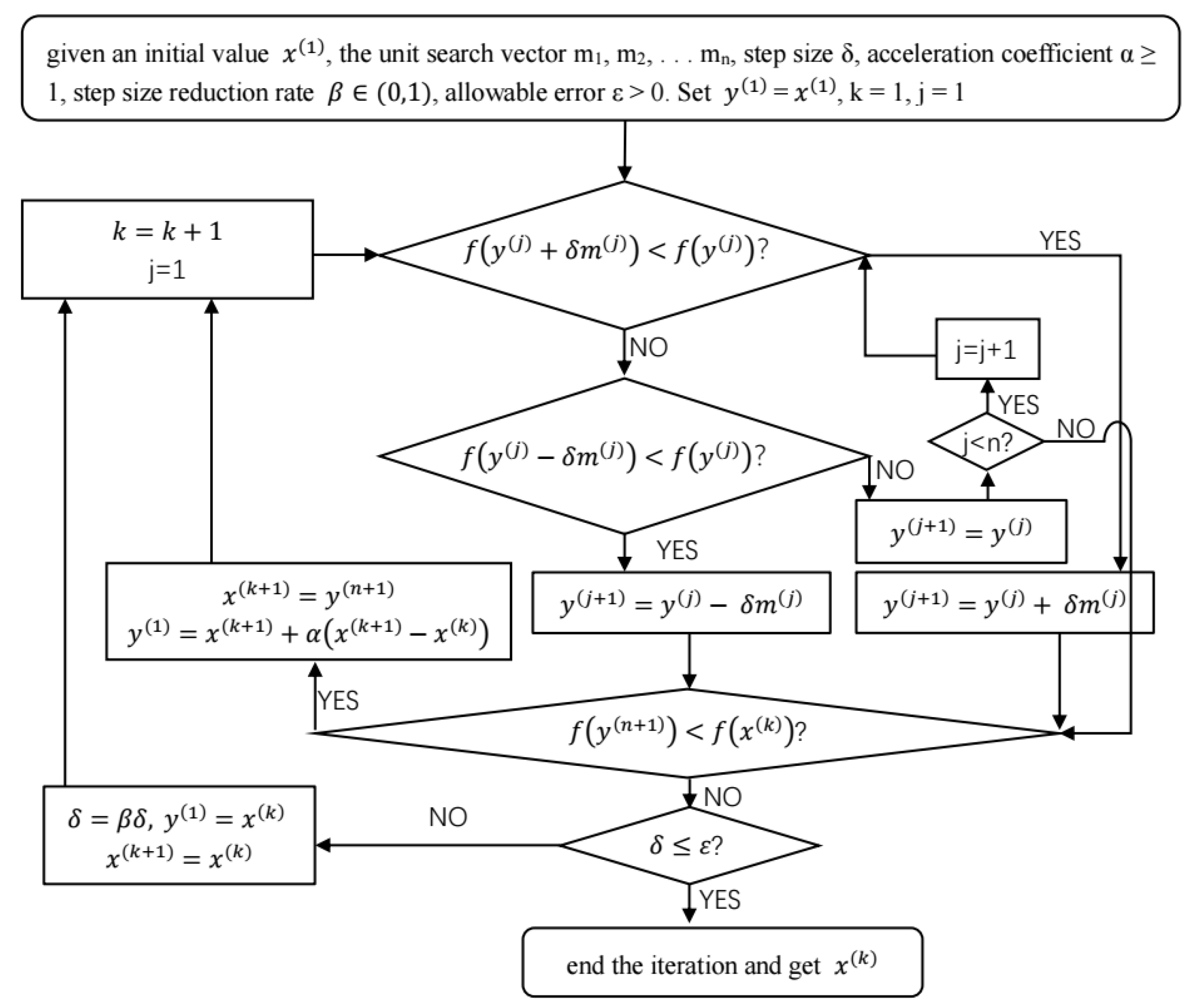
3.3. Parameter Optimization Based on the Monte Carlo Pattern Search Method

The pattern search method, also known as Hooke–Jeeves method, was proposed by Hooke and Jeeves in 1996. The basic idea of the pattern search method is that the algorithm starts from some initial point and alternates between axial and pattern shifts. Since the pattern search method does not require the objective function to be derivable or continuous, it can effectively solve the problem of difficult or non-solvable derivatives. However, the pattern search method can easily fall into a local optimal solution and not find the global optimal solution. In addition, the pattern search method has a strong dependence on the starting base point, and different initial points may lead to different local optimal solutions. To deal with this drawback, the initial points can be generated randomly by the Monte Carlo method. By doing so, the search diversity can be increased, and thus the possibility of finding the global optimal solution can be improved. In this paper, the Monte Carlo pattern search method is implemented by MATLAB (R2021a 9. 10. 0. 1602886): the pattern search method is run for each of the 10,000 initial points generated and the optimal solution is selected as the optimization result from all the results. For an objective function f (x1, x2, …, xn) with n variables, the optimization process of the pattern search method is shown in Figure 2.
The probing movement along m j ( j = 1, 2, ⋯, n) is performed according to the following format:
(1)
Positive axial probing: If f y j + δ m j < f y j , the probe is successful, take y j + 1 = y j + δ m j ; otherwise, the probing fails, and then perform negative axial probing;
(2)
Negative axial probing: If f y j δ m j < f y j , the probe is successful, take y j + 1 = y j δ m j ; otherwise, the probing fails, and y will remain unchanged.
The point obtained after each probing movement is used as the starting point for the next probing movement. After n probing movements, the point that makes the value of f decrease is obtained in general.
The axial search vectors m1, m2, …mn are of the following form:
P I 2 m 1 = 1 , 0 ,   , 0 1 * n m 2 = 0 , 1 ,   , 0 1 * n m n = 0 , 1 ,   , 0 1 * n
The contours of the design parameters of the vibration control system based on a parallel TID at μ 1 = 2.0 are shown in Figure 3. The optimal parameter points in Figure 3 are obtained by MSPS, and some of the codes are shown in Appendix D.

3.4. Parameters in Control Systems Based on Parallel and Serial TID

3.4.1. Inertial Mass Ratio
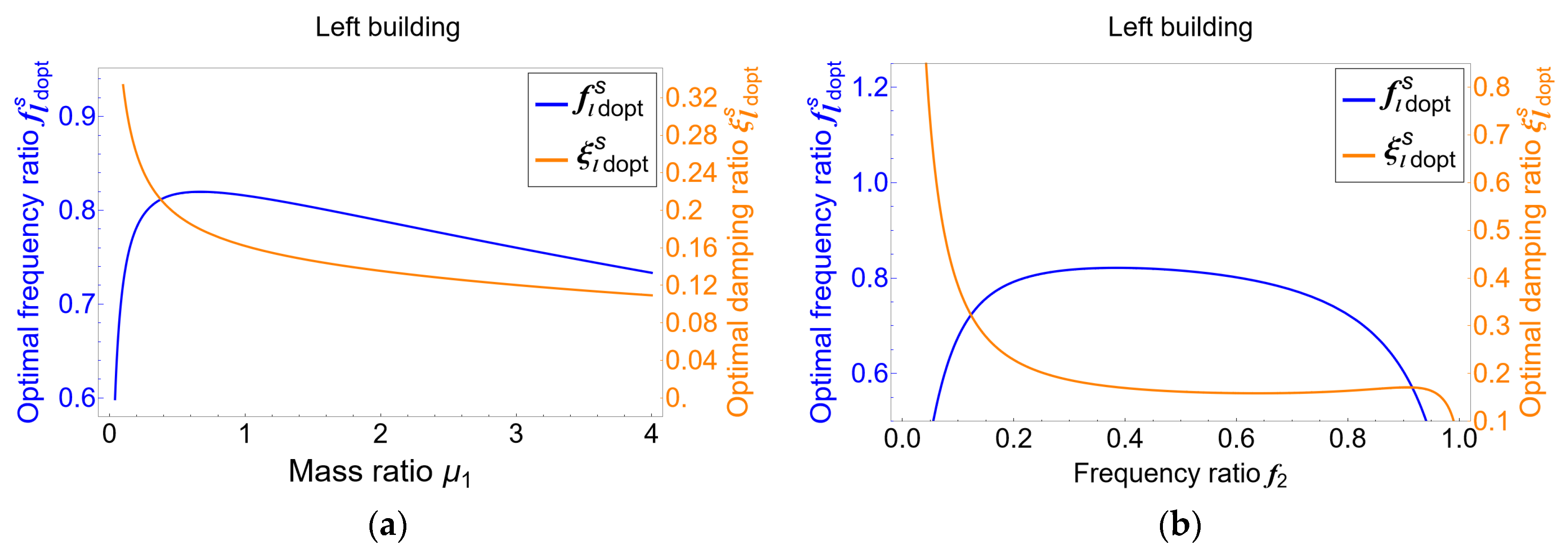
 μ d

The effect of the inertial mass ratio on the amplitude of the frequency response function is shown in Figure 4 by a three-dimensional plot. As the inertial mass ratio increases, the amplitude of the frequency response function decreases significantly in a certain frequency range. However, as the inertial mass ratio increases, the improvement effect gradually decreases. Moreover, the robustness of the system decreases when the inertial mass ratio is too large. Although there is an optimal value of inertial mass ratio for a single TID of a MDOF structure, it is necessary to consider various factors such as economic cost and feasibility in the actual design [44]. Therefore, the design of the vibration control system based on parallel and serial TIDs need to be adjusted and optimized according to the specific situation to ensure the system has a satisfactory seismic performance and economy. In this paper, a more satisfactory result is obtained for both vibration control systems at the inertial mass ratio μ d = 0.1 .
Considering that the masses of adjacent buildings generally do not deviate too much, three mass ratios μ 1 = 1 , μ 1 = 1.5 , μ 1 = 2.0 were selected for comparison. Observing the data in Table 1, it is found that the optimal design parameters of both the left building and the right building in the vibration control system based on parallel TID are significantly higher than those of the vibration control system based on serial TID. In addition, comparing the overall magnitude of change in values reveals that the optimal design parameters ξ d o p t of both systems are most significantly influenced by the mass ratio μ 1 . As the mass ratio μ 1 increases, the damping ratio ξ r p d o p t decreases by 25.21% and 16.37%, and the damping ratio ξ r s d o p t increases by 22.02% and 15.12%, respectively.

3.4.2. Frequency Response Function H l s ( j λ ) and H l p ( j λ )

In this subsection, the frequency response function of the system is solved to obtain the optimal solution for the design parameters. The influence of other parameters on the design parameters is discussed first, followed by a comparative analysis of H l s ( j λ ) and H l p ( j λ ) . The system design parameters are plotted in relation to the mass ratio u at μ 1 = 1 , μ 1 = 1.5 and μ 1 = 2.0 . In Figure 5, the blue line represents f l s d o p t and the orange line represents ξ l s d o p t . From the trend of the curves in Figure 5, it can be seen that the optimal values of the design parameters all decrease as the building mass ratio μ 1 increases.
It can be seen from Figure 6 that the peak value of the response is significantly lower for the vibration control system based on parallel TID, which indicates that the robustness of the vibration control system based on parallel TID is better than that of the vibration control system based on serial TID. At the beginning, as the frequency ratio λ increases, the amplitude of the frequency response function of the vibration control system based on parallel TID is positively correlated with the building mass ratio μ 1 . However, as the frequency ratio λ increases, the increase in the building structure mass ratio μ 1 decreases the vibration suppression effect of the vibration control system. On the whole, the peak value of the frequency response function amplitude of both vibration control systems decreases with the increase of mass ratio μ 1 .
In actual projects, the mass ratio μ 1 of adjacent buildings is not always fixed. In addition, the buildings can cause changes in their own inherent parameters during long-term service, which leads to many devices with large deviations from the ideal values in the practical application of the project. Therefore, it is necessary to consider the extent of the influence of the mass ratio μ 1 and frequency ratio f 2 on the values of design parameters. In Figure 7, the initial phase of the curve shows that the design parameters are both significantly influenced by the building mass ratio μ 1 . One point to note is that the design parameters change less and less as μ 1 increases to a certain level and the curves are flatter. When the frequency ratio f 2 is small, the effect on the design parameters is similar to that of the mass ratio μ 1 . However, when the frequency ratio f 2 grows to a certain value, the optimal value of the design parameters decreases significantly with the increase in the frequency ratio f 2 .

3.4.3. Frequency Response Function H r s ( j λ ) and H r p ( j λ )

In this subsection, the frequency response function H r s ( j λ ) of the system is solved and compared to H r p ( j λ ) . The optimal values of the design parameters in relation to the inertial mass ratio μ d are shown in Figure 8. It is clear that as the inertial mass ratio μ d increases, the less spring stiffness needs to be used to achieve optimal control. As the inertial mass ratio μ d increases, the nonlinearity of the optimal damping ratio ξ d increases and tends to level off. This indicates that when the inertial mass ratio μ d is relatively large, greater damping is required to obtain the optimal vibration reduction performance.
As shown in Figure 9, the effect of increasing the building mass ratio μ 1 on the right building is similar to Section 3.4.2. Initially, as λ increases, the amplitude of the frequency response function of the vibration control system based on parallel TID is positively related to the building mass ratio μ 1 . However, after λ increases to a certain degree, the increase of the building mass ratio μ 1 decreases the vibration reduction effect of the vibration control system. Compared with Figure 6, it can be found that the two vibration control systems are more effective in controlling the vibration of the building on the left.
In this paragraph, building damping ratios ξ l and ξ r are analyzed, and the effects of different damping ratio values on the frequency response functions in the two vibration control systems are explored separately. It can be seen from Figure 10 that an increase in the damping ratio can improve the stability and robustness of the structure, and, overall, an increase in the building damping ratio can better control the structural vibration. Interestingly, the effect of increasing the building damping ratio on the frequency response function of the left building and the right building shows a significant difference. Comparing Figure 10a,b, it can be found that the response peak of the left building decreases as the damping ratio ξ l increases, while the opposite is true for the right building. By comparing Figure 10c,d, the response peak of the left building increases with increasing damping ratio ξ r , while the response peak of the right building is clearly negatively correlated with the damping ratio. When the building damping ratio is used as a variable, interesting things can be found from Figure 10. Although the increasing damping ratio of the left building and the right building is beneficial to them, it is harmful to the neighboring buildings.

4. Verification in the Time Domain

First, these four classical seismic waves EL Centro (1940), Taft (1952), San Fernando (1971) and Northridge (1994) are selected in this paper (see Figure 11). The parameters are set as: mass ratio μ 1 = 2 , inertial mass ratio μ d = 0.1 , frequency ratio f 2 = 0.5 and building damping ratio ξ l = ξ r = 0.1 . For example, one setting of the vibration control system in MATLAB is shown in Table 2. The time domain results of the two vibration control systems are shown in Figure 12 and Figure 13. The peak displacement and dynamic energy of the TID for the building under different seismic excitation for both vibration control systems are listed in Table 3 and Table 4.
In Figure 12, Figure 13 and Figure 14, the blue line represents the response results of the adjacent building structure vibration control system based on parallel TID, the red line represents the response results of the adjacent building structure vibration control system based on serial TID, and the gray line means the response results of the adjacent building structure in the uncontrolled condition. The effectiveness and reliability of the two vibration control systems are evaluated by comparing the results of the above three time history responses. These results help to understand the effects of the two vibration control systems on the seismic performance of building structures and provide references for vibration control in practical engineering. In general, both vibration control systems are able to control the vibration amplitude of the buildings, and are particularly effective in controlling the vibration of the right building. Table 2 shows the peak response of the building structure under four types of seismic excitation for both vibration control systems. Obviously, it is more effective for the vibration control system based on parallel TID to improve the seismic capacity of adjacent building structures. The dynamic energy of the TID in both vibration control systems under EL Centro seismic wave excitation is shown in Figure 14, while the dynamic energy peaks are listed in Table 3. It is obvious that the vibration control system based on serial TID protects the building mainly by converting the seismic energy into dynamic energy. The vibration control system based on parallel TID protects the building mainly by consuming seismic energy through dampers. In the frequency domain analysis, the damping ratio ξ r p d o p t is a little larger in the vibration control system based on parallel TID, which is consistent with the above findings.

5. Conclusions

The paper proposes to connect two adjacent buildings with parallel and serial TIDs, and discusses the seismic performance of the vibration control system based on parallel and serial TIDs. In order to achieve the best vibration reduction effect, the H2 norm theory is used to optimize the design parameters for the vibration control system based on serial TID, and the H2 norm theory and Monte Carlo pattern search method are used to optimize the design parameters for the vibration control system based on parallel TID. The effects of parameter variations on the vibration reduction performance of the two vibration control systems were analyzed and compared. The following conclusions were obtained:
  • When the mass ratios of adjacent buildings in two vibration control systems are close to each other, the amplitude of the frequency response function of the buildings will increase. Therefore, appropriately increasing the mass ratio of adjacent buildings helps to improve the vibration control performance of the system.
  • Compared with the vibration control system based on serial TID, the vibration control system based on parallel TID can not only reduce the amplitude of the frequency response function of the building more effectively, but also apply to a wider range of frequencies.
  • Increasing the damping ratio of the building can effectively improve the amplitude of the frequency response function of the building. When the damping of the building is relatively low, a slight increase in the damping ratio can significantly reduce the amplitude of the frequency response function. However, when the damping ratio of the building is large, it is not worthwhile to continue to increase the damping ratio.
  • Compared with the vibration control system based on serial TID, the vibration control system based on parallel TID has higher robustness and stability. In addition, the vibration control system based on parallel TID can better reduce the vibration amplitude of adjacent buildings under the action of seismic excitation.
  • The vibration control system based on parallel TID dissipates seismic energy mainly by large damping, while the vibration control system based on serial TID protects buildings mainly by converting seismic energy into dynamic energy.

Author Contributions

Conceptualization, X.K. and J.T.; data curation, J.T.; formal analysis, J.T. and J.W. (Jian Wu); investigation, X.K., F.L., J.T. and Q.H.; methodology, X.K., J.T., J.W. (Jiachen Wei) and F.Z.; supervision, X.K. and Q.H.; validation, X.K. and Z.L.; writing—original draft preparation, X.K., J.T. and Z.S.; writing—review and editing, J.T. and F.Z. All authors have read and agreed to the published version of the manuscript.

Funding

This research was funded by the Anhui Provincial Natural Science Foundation (Grant No. 2008085QE245), the Natural Science Research Project of Higher Education Institutions in Anhui Province (Grant No. 2022AH040045), and the Project of Science and Technology Plan of Department of Housing and Urban-Rural Development of Anhui Province (Grant No. 2021-YF22).

Data Availability Statement

No new data were created or analyzed in this study. Data sharing is not applicable to this article.

Conflicts of Interest

The authors declare no conflict of interest.

Appendix A

B 0 p ~ B 4 p and A 0 p ~ A 6 p are the numerator and denominator of the frequency response function H l p ( j λ ) , respectively.
A 6 p = 1 A 5 p = 2   ( ξ l + f 2   ξ r + f d   ξ d ) A 4 p = 1 + f 2 2 + f d 2   ( 1 + μ d + μ 1   μ d ) + 4   f d   ξ l   ξ d + 4   f 2   ξ r   ( ξ l + f d   ξ d ) A 3 p = 2   ( f 2 2   ( ξ l + f d   ξ d ) + f d   ( f d   ( ξ l + μ 1   μ d   ξ l ) + ξ d + f d 2   ( 1 + μ 1 )   μ d   ξ d ) + f 2   ξ r   ( 1 + f d 2   ( 1 + μ d ) + 4   f d   ξ l   ξ d ) ) A 2 p = 4   f 2   f d   ξ r   ( f d   ξ l + ξ d + f d 2   μ d   ξ d ) + f 2 2   ( 1 + f d 2   ( 1 + μ d ) + 4   f d   ξ l   ξ d ) + f d 2   ( 1 + μ 1   ( μ d + 4   f d   μ d   ξ l   ξ d ) ) A 1 p = 2   f d   ( f 2   f d   ξ r + f d 2   μ 1   μ d   ξ d + f 2 2   ( f d   ξ l + ξ d + f d 2   μ d   ξ d ) ) A 0 p = f 2 2   f d 2 B 4 p = 1 B 3 p = 2 ( f 2   ξ r + f d   ξ d ) B 2 p = f 2 2 + f d 2   ( 1 + μ d + μ 1   μ d ) + 4 f 2   f d   ξ r   ξ d B 1 p = 2 f d   ( f 2   f d   ξ r + f 2 2   ξ d + f d 2   ( 1 + μ 1 )   μ d   ξ d ) B 0 p = f 2 2   f d 2
D 0 p ~ D 4 p and C 0 p ~ C 6 p are the numerator and denominator of the frequency response function H r p ( j λ ) , respectively.
C 6 p = 1 C 5 p = 2   ξ l + 2   f 2   ξ r + 2   f d   ξ d C 4 p = 1 + f 2 2 + f d 2 + f d 2   μ d + f d 2   μ 1   μ d + 4   f 2   ξ l   ξ r + 4   f d   ξ l   ξ d + 4   f 2   f d   ξ r   ξ d C 3 p = 2   f 2 2   ξ l + 2   f d 2   ξ l + 2   f d 2 μ 1   μ d   ξ l + 2   f 2   ξ r + 2   f 2   f d 2   ξ r + 2   f 2   f d 2   μ d   ξ r + 2   f d   ξ d + 2   f 2 2   f d   ξ d + 2   f d 3   μ d   ξ d + 2   f d 3   μ 1   μ d   ξ d + 8   f 2   f d   ξ l   ξ r   ξ d C 2 p = f 2 2 + f d 2 + f 2 2   f d 2 + f 2 2   f d 2   μ d + f d 2   μ 1   μ d + f d 4   μ 1   μ d + f d 4   μ 1   μ d 2 f d 4   μ 1   μ d   ( 1 + μ d ) + 4   f 2   f d 2   ξ l   ξ r + 4   f 2 2   f d   ξ l   ξ d + 4   f d 3   μ 1   μ d   ξ l   ξ d + 4   f 2   f d   ξ r   ξ d + 4   f 2   f d 3   μ d   ξ r   ξ d C 1 p = 2   f 2 2   f d 2   ξ l + 2   f d 4   μ 1   μ d   ξ l + 2   f 2   f d 2   ξ r + 2   f 2 2   f d   ξ d + 2   f 2 2   f d 3   μ d   ξ d + 2   f d 3   μ 1   μ d   ξ d + 2   f d 5   μ 1   μ d 2   ξ d 2   f d 4   μ 1   μ d   ( ξ l + f d   μ d   ξ d ) C 0 p = f 2 2   f d 2 D 4 p = 1 D 3 p = 2   ( ξ l + f d   ξ d ) D 2 p = 1 + f d 2   ( 1 + μ d + μ 1   μ d ) + 4   f d   ξ l   ξ d D 1 p = 2   f d   ( f d   ξ l + ξ d + f d 2   ( 1 + μ 1 )   μ d   ξ d ) D 0 p = f d 2

Appendix B

Taking P I l s as an example, the H2 norm performance index is calculated as follows:
P I l s = 1 2 π H l s ( j λ ) 2 d λ = N u m l s D e n l s
where
N u m l s = A 2 s 2   A 5 s ( A 5 s   A 6 s   b 0 + A 0 s   A 1 s   b 5 ) + A 1 s 2   ( A 6 s 3   b 0 + A 0 s   A 6 s 2   b 3 A 0 s   A 4 s   A 6 s   b 4 + A 0 s   A 4 s 2   b 5 ) + A 1 s   ( A 4 s 2   A 5 s   A 6 s   b 0 + A 3 s   A 4 s   A 6 s 2   b 0 + A 0 s   A 4 s   A 5 s   ( A 6 s   b 2 2   A 0 s   b 5 ) + A 0 s   A 6 s   ( A 5 s   A 6 s   b 1 A 3 s   A 6 s   b 2 + A 0 s   A 5 s   b 4 + A 0 s   A 3 s   b 5 ) ) + A 0 s   ( A 3 s   A 5 s   A 6 s   ( A 6 s   b 0 + A 0 s   b 3 ) + A 3 s 2   A 6 s   ( A 6 s   b 1 A 0 s   b 4 ) + A 0 s   A 5 s 2   ( A 6 s   b 2 + A 0 s   b 5 ) + A 4 s   ( A 5 s 2   A 6 s   b 0 A 3 s   A 5 s   A 6 s   b 1 + A 0 s   A 3 s 2   b 5 ) ) A 2 s   ( A 3 s 2   A 6 s 2   b 0 + A 6 s   ( 2   A 1 s   A 5 s   A 6 s   b 0 A 0 s   A 5 s 2   b 1 + A 0 s   A 1 s   A 5 s   b 3 + A 0 s   A 1 s 2   b 5 ) + A 3 s   ( A 4 s   A 5 s   A 6 s   b 0 A 0 s   A 1 s   A 6 s   b 4 + A 0 s   A 1 s   A 4 s   b 5 + A 0 s 2   A 5 s   b 5 ) ) D e n l s = 2   A 0 s   A 6 s   ( A 1 s 3   A 6 s 2 + A 0 s   ( A 3 s 2   A 4 s   A 5 s A 2 s   A 3 s   A 5 s 2 + A 0 s   A 5 s 3 A 3 s 3   A 6 s ) + A 1 s 2   ( A 4 s 2   A 5 s A 3 s   A 4 s   A 6 s 2   A 2 s   A 5 s   A 6 s ) + A 1 s   ( A 2 s 2   A 5 s 2 + A 2 s   A 3 s   ( A 4 s   A 5 s + A 3 s   A 6 s ) + A 0 s   A 5 s   ( 2   A 4 s   A 5 s + 3   A 3 s   A 6 s ) ) ) b 0 = B 0 s 2 b 1 = B 1 s 2 2   B 0 s   B 2 s b 2 = B 2 s 2 2   B 1 s   B 3 s + 2   B 0 s   B 4 s b 3 = B 3 s 2 2   B 2 s   B 4 s b 4 = B 4 s 2 b 5 = 0
where B 0 s ~ B 4 s and A 0 s ~ A 6 s are the numerator and denominator of the frequency response function H l s ( j λ ) .

Appendix C

B 0 s ~ B 4 s and A 0 s ~ A 6 s are the numerator and denominator of the frequency response function H l s ( j λ ) , respectively.
A 6 s = 1 A 5 s = 2 ( ξ l + f 2 ξ r + f d ( 1 + μ d + μ 1 μ d ) ξ d ) A 4 s = ( 1 + f 2 2 + f d 2 ( 1 + μ d + μ 1 μ d ) + 4 f d ( 1 + μ 1 μ d ) ξ l ξ d + 4 f 2 ξ r ( ξ l + f d ( 1 + μ d ) ξ d ) ) A 3 s = 2 ( f d ( 1 + μ 1 μ d ) ( f d ξ l + ξ d ) + f 2 2 ( ξ l + f d ( 1 + μ d ) ξ d ) + f 2 ξ r ( 1 + f d 2 ( 1 + μ d ) + 4 f d ξ l ξ d ) ) A 2 s = ( f d 2 ( 1 + μ 1 μ d ) + 4 f 2 f d ξ r ( f d ξ l + ξ d ) + f 2 2 ( 1 + f d 2 ( 1 + μ d ) + 4 f d ξ l ξ d ) ) A 1 s = 2 f 2 f d ( f d ξ r + f 2 ( f d ξ l + ξ d ) ) A 0 s = f 2 2 f d 2 B 4 s = 1 B 3 s = 2 ( f 2 ξ r + f d ( 1 + μ d + μ 1 μ d ) ξ d ) B 2 s = ( f 2 2 + f d 2 ( 1 + μ d + μ 1 μ d ) + 4 f 2 f d ξ r ξ d ) B 1 s = 2 f 2 f d ( f d ξ r + f 2 ξ d ) B 0 s = f 2 2 f d 2
D 0 s ~ D 4 s and C 0 s ~ C 6 s are the numerator and denominator of the frequency response function H r s ( j λ ) , respectively.
C 6 s = 1 C 5 s = 2 ( ξ l + f 2 ξ r + f d ( 1 + μ d + μ 1 μ d ) ξ d ) C 4 s = ( 1 + f 2 2 + f d 2 ( 1 + μ d + μ 1 μ d ) + 4 f d ( 1 + μ 1 μ d ) ξ l ξ d + 4 f 2 ξ r ( ξ l + f d ( 1 + μ d ) ξ d ) ) C 3 s = 2 ( f d ( 1 + μ 1 μ d ) ( f d ξ l + ξ d ) + f 2 2 ( ξ l + f d ( 1 + μ d ) ξ d ) + f 2 ξ r ( 1 + f d 2 ( 1 + μ d ) + 4 f d ξ l ξ d ) ) C 2 s = ( f d 2 ( 1 + μ 1 μ d ) + 4 f 2 f d ξ r ( f d ξ l + ξ d ) + f 2 2 ( 1 + f d 2 ( 1 + μ d ) + 4 f d ξ l ξ d ) ) C 1 s = 2 f 2 f d ( f d ξ r + f 2 ( f d ξ l + ξ d ) ) C 0 s = f 2 2 f d 2 D 4 s = 1 D 3 s = 2 ( ξ l + f d ( 1 + μ d + μ 1 μ d ) ξ d ) D 2 s = ( 1 + f d 2 ( 1 + μ d + μ 1 μ d ) + 4 f d ξ l ξ d ) D 1 s = 2 f d ( f d ξ l + ξ d ) D 0 s = f d 2

Appendix D

Part of the code for the Monte Carlo pattern search method is as follows:
f_new = rosenbrock(x_new(1), x_new(2));
    if f_new < f_i
      x_i = x_new;
      f_i = f_new;
    end
  end
  if f_i < f_min
    x_min = x_i;
    f_min = f_i;
  end
end

References

  1. Pisal, A.Y.; Jangid, R.S. Vibration control of bridge subjected to multi-axle vehicle using multiple tuned mass friction dampers. Int. J. Adv. Struct. Eng. 2016, 8, 213–227. [Google Scholar] [CrossRef] [Green Version]
  2. Debbarma, R.; Chakraborty, S.; Ghosh, S.K. Optimum design of tuned liquid column dampers under stochastic earthquake load considering uncertain bounded system parameters. Int. J. Mech. Sci. 2010, 52, 1385–1393. [Google Scholar] [CrossRef]
  3. Gao, H.; Kwok, K.; Samali, B. Optimization of tuned liquid column dampers. Eng. Struct. 1997, 19, 476–486. [Google Scholar] [CrossRef]
  4. Ras, A.; Boumechra, N. Seismic energy dissipation study of linear fluid viscous dampers in steel structure design. Alex. Eng. J. 2016, 55, 2821–2832. [Google Scholar] [CrossRef] [Green Version]
  5. Lavan, O.; Levy, R. Optimal design of supplemental viscous dampers for linear framed structures. Earthq. Eng. Struct. Dyn. 2006, 35, 337–356. [Google Scholar] [CrossRef]
  6. Chatzikonstantinou, N.; Makarios, T.K.; Athanatopoulou, A. Integration Method for Response History Analysis of Single-Degree-of-Freedom Systems with Negative Stiffness. Buildings 2022, 12, 1214. [Google Scholar] [CrossRef]
  7. Chang, H.; Liu, L.; Jing, L.; Lu, J.; Cao, S. Study on Damping Performance of Hyperboloid Damper with SMA-Negative Stiffness. Buildings 2022, 12, 1111. [Google Scholar] [CrossRef]
  8. Wang, M.; Sun, F.; Nagarajaiah, S. Simplified optimal design of MDOF structures with negative stiffness amplifying dampers based on effective damping. Struct. Des. Tall Spéc. Build. 2019, 28, e1664. [Google Scholar] [CrossRef]
  9. Kapasakalis, K.A.; Antoniadis, I.A.; Sapountzakis, E.J. Performance assessment of the KDamper as a seismic Absorption Base. Struct. Control Health Monit. 2020, 27, e2482. [Google Scholar] [CrossRef]
  10. Jiang, S.; Bi, K.; Ma, R.; Han, Q.; Du, X. Influence of spatially varying ground motions on the seismic responses of bridge structures with KDampers. Eng. Struct. 2023, 277, 115461. [Google Scholar] [CrossRef]
  11. Lukkunaprasit, P.; Wanitkorkul, A. Inelastic buildings with tuned mass dampers under moderate ground motions from distant earthquakes. Earthq. Eng. Struct. Dyn. 2001, 30, 537–551. [Google Scholar] [CrossRef]
  12. Lavassani, S.H.H.; Kontoni, D.-P.N.; Alizadeh, H.; Gharehbaghi, V. Passive Control of Ultra-Span Twin-Box Girder Suspension Bridges under Vortex-Induced Vibration Using Tuned Mass Dampers: A Sensitivity Analysis. Buildings 2023, 13, 1279. [Google Scholar] [CrossRef]
  13. Farshidianfar, A.; Soheili, S. Ant colony optimization of tuned mass dampers for earthquake oscillations of high-rise structures including soil–structure interaction. Soil Dyn. Earthq. Eng. 2013, 51, 14–22. [Google Scholar] [CrossRef]
  14. Khoshnoudian, F.; Ziaei, R.; Ayyobi, P.; Paytam, F. Effects of nonlinear soil–structure interaction on the seismic response of structure-TMD systems subjected to near-field earthquakes. Bull. Earthq. Eng. 2017, 15, 199–226. [Google Scholar] [CrossRef]
  15. De Angelis, M.; Perno, S.; Reggio, A. Dynamic response and optimal design of structures with large mass ratio TMD. Earthq. Eng. Struct. Dyn. 2011, 41, 41–60. [Google Scholar] [CrossRef]
  16. Hoang, N.; Fujino, Y.; Warnitchai, P. Optimal tuned mass damper for seismic applications and practical design formulas. Eng. Struct. 2008, 30, 707–715. [Google Scholar] [CrossRef]
  17. Jin, L.; Li, B.; Lin, S.; Li, G. Optimal Design Formula for Tuned Mass Damper Based on an Analytical Solution of Interaction between Soil and Structure with Rigid Foundation Subjected to Plane SH-Waves. Buildings 2023, 13, 17. [Google Scholar] [CrossRef]
  18. Kampitsis, A.; Kapasakalis, K.; Via-Estrem, L. An integrated FEA-CFD simulation of offshore wind turbines with vibration control systems. Eng. Struct. 2022, 254, 113859. [Google Scholar] [CrossRef]
  19. Mishra, S.K.; Gur, S.; Chakraborty, S. An improved tuned mass damper (SMA-TMD) assisted by a shape memory alloy spring. Smart Mater. Struct. 2013, 22, 095016. [Google Scholar] [CrossRef]
  20. De Domenico, D.; Ricciardi, G. Earthquake-resilient design of base isolated buildings with TMD at basement: Application to a case study. Soil Dyn. Earthq. Eng. 2018, 113, 503–521. [Google Scholar] [CrossRef]
  21. De Domenico, D.; Ricciardi, G. Improving the dynamic performance of base-isolated structures via tuned mass damper and inerter devices: A comparative study. Struct. Control Health Monit. 2018, 25, e2234. [Google Scholar] [CrossRef]
  22. Salvi, J.; Rizzi, E. Optimum tuning of Tuned Mass Dampers for frame structures under earthquake excitation. Struct. Control Health Monit. 2014, 22, 707–725. [Google Scholar] [CrossRef]
  23. Leung, A.Y.T.; Zhang, H.; Cheng, C.C.; Lee, Y.Y. Particle swarm optimization of TMD by non-stationary base excitation during earthquake. Earthq. Eng. Struct. Dyn. 2008, 37, 1223–1246. [Google Scholar] [CrossRef]
  24. Etedali, S.; Akbari, M.; Seifi, M. MOCS-based optimum design of TMD and FTMD for tall buildings under near-field earthquakes including SSI effects. Soil Dyn. Earthq. Eng. 2019, 119, 36–50. [Google Scholar] [CrossRef]
  25. ABE, M. SEMI-ACTIVE TUNED MASS DAMPERS FOR SEISMIC PROTECTION OF CIVIL STRUCTURES. Earthq. Eng. Struct. Dyn. 1996, 25, 743–749. [Google Scholar] [CrossRef]
  26. Lin, C.-C.; Lin, G.-L.; Wang, J.-F. Protection of seismic structures using semi-active friction TMD. Earthq. Eng. Struct. Dyn. 2009, 39, 635–659. [Google Scholar] [CrossRef]
  27. Xiang, Y.; Tan, P.; He, H.; Chen, Q. Seismic Optimization for Hysteretic Damping-Tuned Mass Damper (HD-TMD) Subjected to White-Noise Excitation. Struct. Control Health Monit. 2023, 2023, 1–21. [Google Scholar] [CrossRef]
  28. Anagnostopoulos, S.A.; Spiliopoulos, K.V. An investigation of earthquake induced pounding between adjacent buildings. Earthq. Eng. Struct. Dyn. 1992, 21, 289–302. [Google Scholar] [CrossRef]
  29. Raheem, S.E.A. Mitigation measures for earthquake induced pounding effects on seismic performance of adjacent buildings. Bull. Earthq. Eng. 2014, 12, 1705–1724. [Google Scholar] [CrossRef]
  30. Xu, Y.; He, Q.; Ko, J. Dynamic response of damper-connected adjacent buildings under earthquake excitation. Eng. Struct. 1999, 21, 135–148. [Google Scholar] [CrossRef]
  31. Abdullah, M.M.; Hanif, J.H.; Richardson, A.; Sobanjo, J. Use of a shared tuned mass damper (STMD) to reduce vibration and pounding in adjacent structures. Earthq. Eng. Struct. Dyn. 2001, 30, 1185–1201. [Google Scholar] [CrossRef]
  32. Su, N.; Peng, S.; Hong, N.; Xia, Y. Wind-induced vibration absorption using inerter-based double tuned mass dampers on slender structures. J. Build. Eng. 2022, 58, 104993. [Google Scholar] [CrossRef]
  33. Bian, Y.; Liu, X.; Sun, Y.; Zhong, Y. Optimized Design of a Tuned Mass Damper Inerter (TMDI) Applied to Circular Section Members of Transmission Towers. Buildings 2022, 12, 1154. [Google Scholar] [CrossRef]
  34. Islam, N.U.; Jangid, R.S. Optimum parameters and performance of negative stiffness and inerter based dampers for base-isolated structures. Bull. Earthq. Eng. 2023, 21, 1411–1438. [Google Scholar] [CrossRef]
  35. Gonzalez-Buelga, A.; Lazar, I.F.; Jiang, J.Z.; Neild, S.A.; Inman, D.J. Assessing the effect of nonlinearities on the performance of a tuned inerter damper. Struct. Control Health Monit. 2017, 24, e1879. [Google Scholar] [CrossRef] [Green Version]
  36. Smith, M. Synthesis of mechanical networks: The inerter. IEEE Trans. Autom. Control 2002, 47, 1648–1662. [Google Scholar] [CrossRef] [Green Version]
  37. Chen, M.Z.; Hu, Y.; Huang, L.; Chen, G. Influence of inerter on natural frequencies of vibration systems. J. Sound Vib. 2014, 333, 1874–1887. [Google Scholar] [CrossRef] [Green Version]
  38. Islam, N.U.; Jangid, R.S. Optimum Parameters of Tuned Inerter Damper for Damped Structures. J. Sound Vib. 2022, 537, 117218. [Google Scholar] [CrossRef]
  39. Kaveh, A.; Farzam, M.F.; Jalali, H.H. Statistical seismic performance assessment of tuned mass damper inerter. Struct. Control Health Monit. 2020, 27, e2602. [Google Scholar] [CrossRef]
  40. Di Matteo, A.; Masnata, C.; Adam, C.; Pirrotta, A. Optimal design of tuned liquid column damper inerter for vibration control. Mech. Syst. Signal Process. 2021, 167, 108553. [Google Scholar] [CrossRef]
  41. Lazar, I.; Neild, S.; Wagg, D. Vibration suppression of cables using tuned inerter dampers. Eng. Struct. 2016, 122, 62–71. [Google Scholar] [CrossRef] [Green Version]
  42. Chen, M.Z.; Papageorgiou, C.; Scheibe, F.; Wang, F.-C.; Smith, M.C. The missing mechanical circuit element. IEEE Circuits Syst. Mag. 2009, 9, 10–26. [Google Scholar] [CrossRef]
  43. Kang, X.; Li, S.; Hu, J. Design and Parameter Optimization of the Reduction-Isolation Control System for Building Structures Based on Negative Stiffness. Buildings 2023, 13, 489. [Google Scholar] [CrossRef]
  44. Shen, W.; Niyitangamahoro, A.; Feng, Z.; Zhu, H. Tuned inerter dampers for civil structures subjected to earthquake ground motions: Optimum design and seismic performance. Eng. Struct. 2019, 198, 109470. [Google Scholar] [CrossRef]
Figure 1. Schematic diagram of the adjacent building structures vibration control systems based on parallel and serial TIDs.
Buildings 13 01803 g001
Figure 2. Optimization process of pattern search method [43].
Buildings 13 01803 g002
Figure 3. Contour plots of frequency ratio and damping ratio ( ξ l = ξ r = 0 , μ d = 0.1 , μ 1 = 2.0 and f 2 = 0.5 ): (a) Left building; (b) Right building.
Buildings 13 01803 g003
Figure 4. Effect of inertial mass ratio on frequency response function ( ξ l = ξ r = 0 , μ 1 = 1.0 and f 2 = 0.5 ): (a) Frequency response function H l p ( j λ ) ; (b) Frequency response function H l s ( j λ ) ; (c) Frequency response function H r p ( j λ ) ; (d) Frequency response function H r s ( j λ ) .
Buildings 13 01803 g004aBuildings 13 01803 g004b
Figure 5. Effect of the inertial mass ratio μ d on the optimal design parameters f l s d o p t and ξ l s d o p t ( ξ l = ξ r = 0 and f 2 = 0.5 ).
Buildings 13 01803 g005
Figure 6. Effect of the mass ratio μ 1 on frequency response function H l s ( j λ ) and H l p ( j λ ) for vibration control systems based on parallel and serial TID ( ξ l = ξ r = 0 and f 2 = 0.5 ).
Buildings 13 01803 g006
Figure 7. (a) Effect of mass ratio μ 1 on optimal values of design parameters ( μ d = 0.1 , f 2 = 0.5 ); (b) Effect of frequency ratio f 2 on optimal values of design parameters ( μ d = 0.1 , μ 1 = 1 ).
Buildings 13 01803 g007
Figure 8. Effect of the inertial mass ratio μ d on the optimal design parameters f r s d o p t and ξ r s d o p t ( ξ l = ξ r = 0 and f 2 = 0.5 ).
Buildings 13 01803 g008
Figure 9. Effect of the mass ratio μ 1 on frequency response function H r s ( j λ ) and H r p ( j λ ) for vibration control systems based on parallel and serial TID ( ξ l = ξ r = 0 and f 2 = 0.5 ).
Buildings 13 01803 g009
Figure 10. The effect of the damping ratio ξ l on the frequency response function ( μ 1 = 2 , μ d = 0.1 , ξ r = 0.02 and f 2 = 0.5 ): (a) Left building; (b) Right building. Effect of damping ratio ξ r on the frequency response function ( μ 1 = 2 , μ d = 0.1 , ξ l = 0.01 and f 2 = 0.5 ): (c) Left building; (d) Right building.
Buildings 13 01803 g010aBuildings 13 01803 g010b
Figure 11. Seismic wave: EL Centro (18 May 1940); Taft (21 July 1952); San Fernando (9 February 1971); Northridge (17 January 1994).
Buildings 13 01803 g011
Figure 12. Displacement of left building under seismic excitation: (a) EL Centro (18 May 1940); (b) Taft (21 July 1952); (c) San Fernando (9 February 1971); (d) Northridge (17 January 1994).
Buildings 13 01803 g012
Figure 13. Displacement of the right building under seismic excitation: (a) EL Centro (18 May 1940); (b) Taft (21 July 1952); (c) San Fernando (9 February 1971); (d) Northridge (17 January 1994).
Buildings 13 01803 g013
Figure 14. Dynamic energy of TID under the action of EL Centro: (a) Left building; (b) Right building.
Buildings 13 01803 g014
Table 1. Optimization results of design parameters for vibration control system based on parallel and serial TIDs.
Mass   Ratio   μ 1 f l p d o p t ξ l p d o p t f r p d o p t ξ r p d o p t f l s d o p t ξ l s d o p t f r s d o p t ξ r s d o p t
11.7141.1361.8800.8250.8160.1620.4780.168
1.51.5661.1201.9960.6170.8030.1460.4640.205
21.4281.1181.9920.5160.7890.1350.4510.236
Table 2. The parameters of a vibration control system based on parallel TID in MATLAB.
ParametersLeft BuildingRight BuildingSerial TID
Mass (or inertance) (kg) 3.5382 × 10 4 1.7691 × 10 4 3.5382 × 10 3
Damping (kN∙s/m) 2.245268 × 10 5 5.613169 × 10 4 3.584579 × 10 5
Stiffness (kN/m) 3.562 × 10 7 4.4525 × 10 6 7.263573408 × 10 6
Table 3. Peak of time history response.
EarthquakePeak Displacement of the Left Building (m)Peak Displacement of the Right Building (m)
ParallelSerialParallelSerial
EL Centro0.0062689760.0064569390.0139435370.017472398
Taft0.002739250.00287410.005464030.00981471
San Fernando0.004949720.005943650.01052610.01917793
Northridge0.00496130.00574070.011699960.01555647
Table 4. Dynamic energy of TID.
EarthquakeDynamic Energy of TID at Optimizing the Left Building (J)Dynamic Energy of TID at Optimizing the Right Building (J)
ParallelSerialParallelSerial
EL Centro37.33402959434.207969765.37584434378.3601604
Taft5.669300497.412911911.657539193.0073466
San Fernando32.0653859318.24910573.7418221247.6958092
Northridge4.3210444330.316168149.7483858270.1696667
Disclaimer/Publisher’s Note: The statements, opinions and data contained in all publications are solely those of the individual author(s) and contributor(s) and not of MDPI and/or the editor(s). MDPI and/or the editor(s) disclaim responsibility for any injury to people or property resulting from any ideas, methods, instructions or products referred to in the content.

