Clustering of Asphalt Pavement Maintenance Sections Based on 3D Ground-Penetrating Radar and Principal Component Techniques

Abstract

Asphalt pavement maintenance section classification is an important prerequisite for accurately determining asphalt pavement maintenance needs and formulating accurate maintenance plans. This paper introduces the three-dimensional (3D) ground-penetrating radar (GPR) pavement internal crack rate index on the basis of an original road surface performance data matrix, and the dimensionality of the road section classification data matrix was reduced through the principal component technique. An analysis of variance was used to compare the significance of the differences in the results for road section classification using different clustering methods and different clustering data and to investigate the influence of the clustering method, principal component technique and crack rate index on the maintenance road section classification results. The results showed that the principal component technique could reduce the dimensionality of the data matrix by 33% and retain more than 84% of the information. There was a genetic relationship between the clustering data and the technical characteristics of the classified sub-sections, and the internal crack rate was important for the characterisation of internal defects in asphalt pavement sub-sections and the determination of maintenance needs. The results of section classification varied considerably between clustering methods, and the choice of clustering method had a relationship to the pavement maintenance objectives. The dynamic clustering method combined with principal component analysis could significantly improve the significance of the differences in the clustering results, effectively improving the division of maintenance sections.

1. Introduction

1.1. Background

Maximising technical and economic benefits is the ultimate goal of scientific decision making for preventive maintenance [1,2]. The scientific decision, which is mainly about applying the right preventive maintenance measures in the right place at the right time, usually includes the determination of the maintenance timing, the division of maintenance intervals and the selection of maintenance solutions [3,4]. Segmenting is an important technical tool to differentiate the maintenance needs of different segments and to allocate maintenance resources appropriately [5,6,7].

The initial division of asphalt pavement preventive maintenance sections is usually based on geology, weather, traffic, bridging, culverting, tunnel structure distribution and other spatial characteristics, with the same external condition characteristics of the various components of the road section being pre-divided into categories [8,9,10]. This method is still used in current maintenance management practice due to its simplicity of operation, but the results of section classification are fixed. It is difficult to relate this classification to the variability of external conditions, pavement disease characteristics (especially internal pavement disease characteristics), etc. With the development of preventive maintenance techniques [11,12], scholars have undertaken more in-depth research on the classification of maintenance sections, and the importance of asphalt pavement distress characteristics in section classification has increased [13,14,15]. The development of more efficient classification algorithms has become a major research hotspot, aiming to help fully exploit the differentiated information for asphalt pavement sections [16,17,18].

The above research has greatly contributed to the advancement of scientific decision making in preventive maintenance plans but still remains at the level of using surface functional indicators as the basis. These studies have limitations because internal pavement distress is easily covered by frequent preventive maintenance and surface indicators do not fully reflect the whole pavement condition [19,20]. Although methods for determining the preventive or structural maintenance needs of different road sections have been proposed [21,22], in practice, it is often found that several road sections that have been determined to be in need of preventive maintenance require preventive maintenance of different intensity or with different capacity levels because of the differences in the internal condition of these sections. Unfortunately, the technical indicators on which decision making about asphalt pavement maintenance plans is based do not so far include indicators of pavement internal damage, such as cracks, and relevant studies are less common [8,23,24,25].

When a certain clustering algorithm is used for a certain set of clustered data, the optimal classification result can be obtained from the iteration of the algorithm, but the samples under different classes do not necessarily have statistically significant differences, and it is difficult to match the pavement maintenance decision-making plan with the actual demand. This problem reduces the reliability of the classification results for asphalt pavement maintenance sections. Unfortunately, while previous studies have focused on the improvement of specific algorithms’ own classification effects, there is a lack of in-depth research on the composition of clustering data, the choice of clustering methods and the relationship between them [26,27,28].

1.2. Objective and Scope

The objectives of this study were first to adopt the three-dimensional GPR-based pavement internal crack rate index and the principal component technique to realize the segmentation of asphalt pavement maintenance sections and secondly to analyse the influence of different clustering methods and clustering data on the classification results. This will provide a theoretical basis for the determination of the basic data indicators and the selection of clustering methods for the classification of asphalt pavement and enable a more scientific classification of maintenance sections.

2. Methods

Cluster analysis is a method of classifying research objects without knowing how many classes they should be divided into using the help of statistical methods and based on the information already collected. The method of clustering analysis is to find some statistical quantities that objectively reflect the relationship between the research objects and their proximity. There are three main methods of cluster analysis: systematic clustering, dynamic clustering and ordered clustering [29,30].

2.1. Systematic Clustering Methods

The systematic clustering method, also named the hierarchical clustering method [31,32], is one of the most widely used all around the world. It involves first looking at the clustered samples or variables as specific groups, determining the similarity statistics between classes, selecting the two closest classes or a number of classes to merge into a new class, calculating the similarity statistics between the new class and the other classes, and then selecting the two closest clusters or a number of clusters to merge into a new class until all the samples or variables are combined into one class. The specific steps for classifying road sections using the systematic clustering method are as follows:

Step 1: The project is pre-divided into $n$ unit sections according to a fixed length $l_0$. For each unit section, a sample set of $m$ disease indicators is collected to form the sample set $X\left(n\times m\right)$ for the maintenance project, as shown by Equation (1):

$$X=\left\{x_{ij}\right\}=\left[\begin{array}{ccc}{x}_{11}& \cdots & x_{1m}\\ ⋮& \ddots & ⋮\\ x_{n1}& \cdots & x_{nm}\end{array}\right],\left(i=1,2,\dots ,n;j=1,2,\dots ,m\right)$$

(1)

where $x_{ij}$ is the $m\mathrm{t}\mathrm{h}$ disease characteristic indicator in the $n$th unit section.

Due to the variation in the range of values for each disease characteristic indicator, $x_{ij}$ is dimensionless for mathematical purposes, as shown by Equation (2):

$${x_{ij}}^{*}=\frac{x_{ij}-\overline{x_j}}{s_j},\left(i=1,2,\dots ,n;j=1,2,\dots ,m\right)$$

(2)

where $\overline{x_j}$ is the mean of each characteristic variable, and $s_j$ is the standard deviation.

The dimensionless sample set $X^{*}$ is calculated according to Equation (3):

$$X^{*}=\left[\begin{array}{ccc}{x_{11}}^{*}& \cdots & {x_{1m}}^{*}\\ ⋮& \ddots & ⋮\\ {x_{n1}}^{*}& \cdots & {x_{nm}}^{*}\end{array}\right]$$

(3)

Step 2: The distance $d_{ij}$ between two sections of the $n$th unit is calculated.

Defining each of the $n$ unit sections as a class, the number of classes for all the unit sections is $l=n,$ and the matrix $Y$ of sections of the conservation project is shown in Equation (4):

$$Y=\left\{{X_i}^{*}\right\},\left(i=1,2,\dots ,n\right)$$

(4)

The distance $d_{i{i}^{\prime }}$ between two sections of the $n$th unit can be calculated using Equation (5):

$$d_{i{i}^{\prime }}=\frac{1}{m}{\sum }_{j=1}^m\left|{x_{ij}}^{*}-{x_{i^{\prime }j}}^{*}\right|,\left(i,i^{\prime }=1,2,\dots ,n\right)$$

(5)

Step 3: The two closest classes in the matrix $Y$ are merged into one new class, and the number of classes in all unit sections of the combined project becomes $l=n-1$. Then, in the new class, it is necessary to continue to find the two closest classes to merge and to repeatedly merge them until the classification ends when the number of divided sections reaches the target $l=t$. When a new class contains at least two unit sections, the distance between the classes is calculated according to Equation (6):

$$d_{RS}=\sqrt{\frac{1}{n_R{n}_S}{\sum }_{i\in Y_R,i^{\prime }\in Y_S}{d_{i{i}^{\prime }}}^2},\left(n_R\ge 1,n_S\ge 1\right)$$

(6)

where $d_{RS}$ is the distance between two new classes, $Y_R$ and $Y_S$; and $n_R$ and $n_S$ are the number of unit sections contained in them, respectively.

2.2. Dynamic Clustering Methods

The dynamic clustering method involves randomly selecting a group of coalescence points, letting the other samples coalesce towards the coalescence points according to some principle (usually the minimal Euclidean distance) and iterating on the coalescence points until the coalescence points are stable. A popular dynamic clustering method is the k-means method [33,34].

The specific steps for classifying road sections using dynamic clustering are as follows:

Step 1: The dimensionless processing of the raw data matrix is consistent with the systematic clustering approach;

Step 2: The number of categories $t$ is specified and a random sample of $X^{*}$ is selected as the cluster centre ${\delta }_c$ for each category.

$${\delta }_c=\left({\delta }_{c_1},{\delta }_{c_2},\dots ,{\delta }_{c_t}\right)$$

(7)

$${\delta }_{c_k}=\left({x_{{\xi }_{k}1}}^{*},{x_{{\xi }_{k}2}}^{*},\dots ,{x_{{\xi }_{k}m}}^{*}\right),\left(k=1,2,\dots ,t; {\xi }_k=index\left({X_i}^{*},randbetween\left(1,n\right)\right)\right)$$

(8)

where ${\xi }_k$ is the serial number of the randomly selected sample in $X^{*}$;

Step 3: The distance of each sample in $X^{*}$ from each cluster centre ${\delta }_{c_k}$ is calculated.

$$d_{{ic}_k}=\sqrt{{\sum }_{j=1}^m{\left({x_{ij}}^{*}-{\delta }_{c_{k}j}\right)}^2},\left(i=1,2,\dots ,n; k=1,2,\dots ,t\right)$$

(9)

Step 4: All samples with the smallest distance from ${\delta }_{c_k}$ in $X^{*}$ are combined into one set (the set $t$ can be obtained), and the updated cluster centres for each set are recalculated. The cluster centres are determined using an iterative calculation, and the cluster centres obtained in the $\eta$th iteration are denoted as ${{\delta }_{c_k}}^{\left(\eta \right)}$.

$${{\delta }_{c_k}}^{\left(\eta \right)}=\frac{1}{N_k}{\sum }_{i=1}^{N_k}{x_{ij}}^{*},\left(j=1,2,\dots ,m; k=1,2,\dots ,t\right)$$

(10)

where $N_k$ is the number of samples in the new set $k$;

Step 5: The final clustering result is obtained when the samples in the set corresponding to the update of the clustering centre ${{\delta }_{c_k}}^{\left(\eta +1\right)}$ for the step $\eta +1$ match the samples in the set corresponding to the $\eta$th step clustering centre ${{\delta }_{c_k}}^{\left(\eta \right)}$.

2.3. Ordered Clustering Methods

Compared to systematic clustering methods in terms of sample data capacity, dynamic clustering methods have a greater range of application. However, both the methods disrupt the original unit sections denoted by asphalt pavement serial numbers; for example, the unit sections numbered 1, 3, 5 and 7 are classified as the first category, while the unit sections numbered 2, 4, 6 and 8 are classified as the second category. The two types of maintenance needs are different and require different maintenance programs. They must be constructed in phases, which greatly increases the difficulty of implementing maintenance construction, especially for projects with high traffic volumes, as well as increasing the frequency and reducing the efficiency of the deployment of construction equipment and other resources. Ordered clustering methods, also called optimal partitioning methods, can achieve a constant front-to-back order for each unit section [35,36]. The specific steps of the ordered clustering method are as follows:

Step 1: The dimensionless processing of the raw data matrix is consistent with the systematic clustering approach;

Step 2: The number of categories $t$ is specified. It is assumed that one of the category is $C_{i{i}^{\prime }}$, which is listed in Equation (11):

$$C_{i{i}^{\prime }}=\left\{{x_i}^{*},{x_{i+1}}^{*},\dots ,{x_{i^{\prime }}}^{*}\right\},\left(i^{\prime }>i\right)$$

(11)

The mean value of $C_{i{i}^{\prime }}$ is calculated using Equation (12):

$$\overline{x_{l{l}^{\prime }}}=\frac{1}{i^{\prime }-i+1}{\sum }_{\zeta =i}^{i^{\prime }}{x_{\zeta }}^{*}$$

(12)

The diameter $D_{i{i}^{\prime }}$ of each category of $C_{i{i}^{\prime }}$ is calculated using Equation (13):

$$D_{i{i}^{\prime }}={\sum }_{\zeta =i}^{i^{\prime }}{\left({x_{\zeta }}^{*}-\overline{x_{l{l}^{\prime }}}\right)}^{\prime }\left({x_{\zeta }}^{*}-\overline{x_{l{l}^{\prime }}}\right)$$

(13)

Step 3: The objective function is calculated.

A particular classification scheme is $C\left(n,t\right):\left\{i^{\prime },i+1,\dots ,i_2-1\right\},\left\{i_2,i_2+1,\dots ,i_3-1\right\},\dots ,\left\{i_t,i_t+1,\dots ,n\right\}$; then, the objective function is as shown by Equation (14):

$$e\left[C\left(n,t\right)\right]={\sum }_{k=1}^{t-1}D\left(i_k,i_{k+1}-1\right)$$

(14)

When $n$ and $t$ are fixed, the smaller $e\left[C\left(n,t\right)\right]$ is, the smaller the sum of squares of the deviations of each class is and the more reasonable the classification.

$e\left[C\left(n,t\right)\right]$ is calculated using the recursive Equations (15) and (16):

$$e\left[C\left(n,2\right)\right]=\underset{2\le i\le n}{\mathit{min}}\left\{D\left(1,i-1\right)+D\left(i,n\right)\right\}$$

(15)

$$e\left[C\left(n,t\right)\right]=\underset{t\le i\le n}{\mathit{min}}\left\{e\left[C\left(i-1,t-1\right)\right]+D\left(i,n\right)\right\}$$

(16)

Step 4: The optimal classification is calculated.

Under the condition that the number of categories $t$ is set, $i_t$ can be found such that the objective function $e\left[C\left(n,t\right)\right]$ is minimised.

$$e\left[C\left(n,t\right)\right]=e\left[C\left(i_t-1,t-1\right)\right]+D\left(i_t,n\right)$$

(17)

The classification $C_t=\left\{{x_{i_t}}^{*},{x_{i_t+1}}^{*},\dots ,{x_n}^{*}\right\}$ is obtained. Further, $i_t-1$ is found and $e\left[C\left(i_t-1,k-1\right)\right]$ can be calculated using Equation (18):

$$e\left[C\left(i_t-1,k-1\right)\right]=e\left[C\left(i_{t-1}-1,t-2\right)\right]+D\left(i_{t-1},i_t-1\right)$$

(18)

Thus, we obtain $C_{t-1}=\left\{{x_{i_{t-1}}}^{\mathrm{*}},{x_{i_{t-1}+1}}^{\mathrm{*}},\dots ,{x_{i_t-1}}^{\mathrm{*}}\right\}$. All categories $C_k,\left(k=1,2,\dots ,t\right)$ can be obtained by analogy.

3. Data Collection

In order to obtain more accurate unit section maintenance requirements for maintenance section classification, this paper proposes a technical condition evaluation index system that includes both pavement surface and pavement internal disease characteristics. The pavement surface technical condition indicators include the pavement condition index ($PCI$), skid resistance index ($SRI$), rut depth index ($RDI$) and ride quality index ($RQI$). The technical indicators for the characterisation of internal pavement distress are the internal pavement crack rate indicators. The length of a unit section in this paper is set to 1000 m [37].

3.1. Project and Materials

This research was based on an expressway named GB1 that was opened to traffic in 2005; it is an important highway section of the Beijing–Hong Kong–Macau Expressway in Guangdong province. The traffic volume has increased rapidly to the current average of 120,000 vehicles per day (converted to passenger cars). Traffic congestion is becoming more and more normal, especially during holidays.

Table 1. Pavement structure information for a typical section.

Layer	Definition
Asphalt overlay	0.5–2 cm preventive maintenance measures
Upper layer (asphalt)	5 cm AK-16 (with base binder asphalt)
Middle layer (asphalt)	6 cm AC-20 (with base binder asphalt)
Lower layer (asphalt)	7 cm AC-25 (with base binder asphalt)
Base layer	38 cm stabilized gravel (cement content: 5–6%)
Sub-base layer	16 cm stabilized gravel (cement content: 4%)
Subgrade	Soil

provides some information on the structure of a typical section. The upper layer of the pavement structure is a 5 cm AK-16 anti-skid wear layer, while the middle layer and lower layer adopt the widely used continuous dense-gradation 6 cm AC-20 and 7 cm AC-25 materials, respectively. The base layer is almost 54 cm of cement-stabilized gravel. In the last five years, some 0.5–2 cm ultra-thin overlays have been successively paved on the upper layer, such as Novachip.

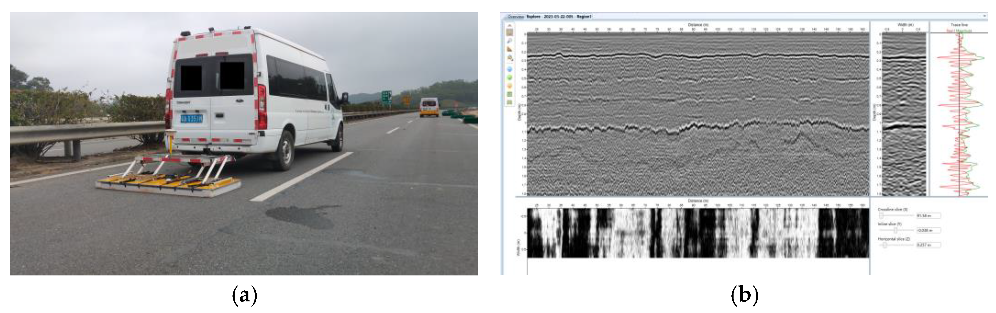
3.2. Data Collection for the Surface Technical Condition

The multifunctional vehicle mainly consisted of a charge-coupled device (CCD) camera system, laser scanner system, GPS system and distance measuring device (DMI). The CCD camera with a resolution of 1920 × 1080 pixels could simultaneously record images at different angles and identify different kinds of surface diseases. The surveying width was more than 4 m. The vehicle could detect one time period during which the full width of each lane with a width of 3.75 m could be covered in a continuous project. The vehicle speed during detection ranged from 60 km/h to 80 km/h.

The multifunctional vehicle could simultaneously determine the three surface condition indexes (pavement condition index ($PCI$), rut depth index ($RDI$) and riding quality index ($RQI$)), while the skid resistance index ($SRI$) required a special sideway-force coefficient detection vehicle.

3.3. Data Collection for the Pavement Internal Crack Rate

This project used 3D GPR to detect the inner damage affecting pavement structures [38,39]. The 3D GPR used was produced by 3D Radar (Trondheim, Norway) as Figure 1a). The radar host was GEOSCOPE MK IV, and the ground-coupled antennas were the DXG1820 model with a frequency bandwidth of 200–3000 MHz. The utilized 3D GPR could provide 20 emitting and receiving channels for electromagnetic wave signals through a linear combination of 20 pairs of antennas. The separation between antennas was 7.5 cm and the single sampling width for the GPR was 1.5 m. Changes in the GPR’s detection parameters caused variations in the vehicle speed during data collection, and the general vehicle speed ranged from 5 km/h to 60 km/h. The trigger spacing was 1 cm, dwell time was 10.0 µs and the time window was 25 ns [19]. The software used to process the 3D GPR data was 3D-Radar Examiner 3.5 as Figure 1b).

The pavement internal crack rate was utilized to characterize the cracks of the unit sections and calculated using Equation (19) [19]:

$$Cr\left(i\right)=50{lc}_i/S_i$$

(19)

where $Cr\left(i\right)$ is the pavement internal crack rate at the depth of $h_i$ (m/100 m²). ${lc}_i$ is the length of the cracks within a surveying section at the depth of $h_i$ (m). $S_i$ is the surveying area at the depth of $h_i$ (m²).

4. Results and Analysis

In this paper, data for 46 unit sections from the GB1 project were collected using a multifunctional vehicle, sideway-force coefficient detection vehicle and 3D GPR equipment (see

Table 2. Pavement condition index.

Unit Section Number	$\mathit{P}\mathit{C}\mathit{I}$	$\mathit{S}\mathit{R}\mathit{I}$	$\mathit{R}\mathit{D}\mathit{I}$	$\mathit{R}\mathit{Q}\mathit{I}$	$\mathit{C}\mathit{r}\mathbf{\left(}\mathbf{0}\mathbf{\right)}$	$\mathit{C}\mathit{r}\mathbf{\left(}\mathbf{0.25}\mathbf{\right)}$
1	74	96	84	94	53.0	26.0
2	74	96	84	94	53.0	28.0
3	76	99	82	93	0.0	39.0
4	86	99	82	97	28.7	45.0
5	86	100	85	95	20.5	37.0
6	86	100	85	95	20.5	18.0
7	86	100	85	95	20.5	79.0
8	86	100	85	95	20.5	3.0
9	80	100	83	95	18.8	28.0
10	80	100	83	95	18.8	65.0
11	80	100	83	95	18.8	0.0
12	86	98	83	95	9.0	14.0
13	82	99	84	94	15.1	12.0
14	82	99	84	94	15.1	56.0
15	80	99	85	94	15.5	74.0
16	80	99	85	94	15.5	65.0
17	85	99	84	95	11.7	57.0
18	85	99	84	95	11.7	44.0
19	88	97	83	95	17.7	50.0
20	97	99	82	93	14.5	57.0
21	97	99	82	93	14.5	45.0
22	93	98	84	95	7.1	38.0
23	93	98	84	95	7.1	11.0
24	93	98	84	95	7.1	31.0
25	87	93	81	95	15.5	42.0
26	87	93	81	95	15.5	21.0
27	85	98	84	96	14.4	6.0
28	84	98	83	95	14.0	50.0
29	90	98	85	93	8.1	9.0
30	90	98	85	93	8.1	39.0
31	84	98	82	93	12.2	73.0
32	100	93	82	97	4.5	44.0
33	94	98	85	95	12.4	2.0
34	100	97	84	94	4.1	59.0
35	100	97	84	94	4.1	79.0
36	93	99	83	95	12.9	20.0
37	81	98	85	94	14.8	37.0
38	81	98	85	94	14.8	25.0
39	81	98	85	94	14.8	32.0
40	88	98	84	94	13.9	5.0
41	93	98	84	94	10.0	41.0
42	93	98	84	94	10.0	74.0
43	93	98	84	94	10.0	77.0
44	93	98	84	94	10.0	39.0
45	100	100	82	95	0.2	43.0
46	96	96	85	98	0.0	47.0

). According to previous studies [40], the life of a semi-rigid-base asphalt pavement is mainly composed of the fatigue cracking life of the semi-rigid base and the fatigue cracking life of the asphalt layer, which is influenced by the integrity (cracking state) of the structural layer. Therefore, this study used the asphalt surface crack rate $Cr\left(0\right)$ and the base layer’s crack rate as indicators for evaluating the maintenance needs of a unit section. The sum thickness of the whole asphalt layer and the ultra-thin overlay plus 0.05 m was taken as the radar signal pick-up depth for the base layer. Data collected from the GB1 project are listed in Table 2.

4.1. Principal Components Analysis

There is often a certain correlation between the pavement performance indicators during service life; for example, ride quality indicators are often influenced by rutting indicators. This eliminates the requirement to subject all the metrics collected to calculation to assess the need for pavement maintenance, saving computing resources. The principal component analysis (PCA) technique is a commonly used method of data dimensionality reduction [41,42].

(1)

Applicability test for PCA

Principal component factor analysis was performed for the six technical indicators (shown in Table 2) in this study using the Kaiser–Meyer–Olkin test and Barlett’s test of sphericity [43]. The test model is shown by Equation (20):

$$KMO=\left\{\begin{array}{c}\ge 0.5,OK\\ <0.5,NotOK\end{array}\right.,\left(KMO=\frac{\sum \sum _{i\ne j}{r_{ij}}^2}{\sum \sum _{i\ne j}{r_{ij}}^2+\sum \sum _{i\ne j}{{\alpha }_{ij}}^2}\right)$$

(20)

where $r_{ij}$, and ${\alpha }_{ij}$ are, respectively, the simple and bias correlation coefficients for each pair of indicators in Table 2. The correlation matrix for the PCA is shown in

Table 3. Correlation matrix for PCA.

Correlation Coefficient	$\mathit{P}\mathit{C}\mathit{I}$	$\mathit{S}\mathit{R}\mathit{I}$	$\mathit{R}\mathit{D}\mathit{I}$	$\mathit{R}\mathit{Q}\mathit{I}$	$\mathit{C}\mathit{r}\mathbf{\left(}\mathbf{0}\mathbf{\right)}$	$\mathit{C}\mathit{r}\mathbf{\left(}\mathbf{0.25}\mathbf{\right)}$
$PCI$	1.000	0.162	−0.136	−0.181	−0.617	0.158
$SRI$	0.162	1.000	−0.074	−0.206	−0.044	−0.143
$RDI$	−0.136	−0.074	1.000	0.341	0.064	−0.082
$RQI$	−0.181	−0.206	0.341	1.000	−0.033	0.011
$Cr\left(0\right)$	−0.617	−0.044	0.064	−0.033	1.000	−0.153
$Cr\left(0.25\right)$	0.158	−0.143	−0.082	0.011	−0.153	1.000
Significance	$PCI$	$SRI$	$RDI$	$RQI$	$Cr\left(0\right)$	$Cr\left(0.25\right)$
$PCI$		0.141	0.184	0.115	0.000 a	0.146
$SRI$	0.141		0.312	0.084	0.386	0.171
$RDI$	0.184	0.312		0.010 b	0.337	0.293
$RQI$	0.115	0.084	0.010 b		0.414	0.472
$Cr\left(0\right)$	0.000 a	0.386	0.337	0.414		0.154
$Cr\left(0.25\right)$	0.146	0.171	0.293	0.472	0.154

Note: ^a significance p-value < 0.01, ^b significance p-value < 0.05.

.

As can be seen from Table 3, the absolute values of the cross-correlation coefficients for the six technical indicators ranged from 0.033 to 0.617, with the correlation coefficient between $PCI$ and $Cr\left(0\right)$ being the largest and most significant; thus, it can be presumed that the main surface disease affecting the GB1 project is cracking. Secondly, the correlation between $RDI$ and $RQI$ was also somewhat significant, in line with the engineering understanding that rutting has some effect on the ride quality provided by a road surface. The result of the $\mathrm{K}\mathrm{M}\mathrm{O}$ test was 0.517 > 0.5 and the result of Barlett’s test of sphericity was $p<0.05$ (p value of 0.003), thus, the six technical indicators were judged to be suitable for principal component analysis.

(2)

Principal component retention

The GB1 measured sample data matrix $\mathrm{X}=\left\{X_j\right\},\left(j=1,2,\dots ,6\right)$ was normalized according to Equation (2) to obtain $X^{*}=\left\{{X_j}^{*}\right\},\left(j=1,2,\dots ,6\right)$. Then, we calculated the data correlation matrix $R\left(X^{*}\right)=R\left(X\right)$ (see Table 3). The eigenvalues of $R\left(X^{*}\right)$ were calculated from $\left|R\left(X^{*}\right)-\lambda E\right|=0$ and are shown in

Table 4. Eigenvalues of correlation matrix.

Principal Component	$\mathbf{Eigenvalues},{\mathit{\lambda }}_{\mathit{j}}$	$\mathbf{Cumulative}\mathbf{Contribution}\mathbf{Rate},{\mathbf{c}}_{\mathsf{\varsigma }}\mathbf{/}\mathbf{\%}$
Z1	1.808	30.128
Z2	1.362	52.826
Z3	1.089	70.974
Z4	0.761	83.662
Z5	0.637	94.278
Z6	0.343	100.000

. Each eigenvalue corresponded to a principal component $Z_{\varsigma },(\varsigma =1,2,\dots ,6)$, and the cumulative contribution of $Z_{\varsigma }$ was calculated from ${\mathrm{c}}_{\mathsf{\varsigma }}={\sum }_{j=1}^{\varsigma }{\lambda }_j/{\sum }_{j=1}^6{\lambda }_j$ (see Table 4). The eigenvectors corresponding to the eigenvalues of $R\left(X^{*}\right)$ were also calculated from $\left|R\left(X^{*}\right)-\lambda E\right|=0$, and the eigenvectors are listed in

Table 5. Eigenvectors corresponding to the eigenvalues.

Index	Z1	Z2	Z3	Z4	Z5	Z6
E1*	0.632	0.190	−0.180	0.089	0.171	0.704
E2*	0.227	−0.419	−0.539	−0.605	−0.334	−0.071
E3*	−0.324	0.417	−0.474	−0.326	0.622	−0.053
E4*	−0.311	0.584	−0.204	0.011	−0.683	0.233
E5*	−0.549	−0.397	0.204	−0.231	0.072	0.664
E6*	0.216	0.340	0.608	−0.683	−0.014	−0.041

.

From Table 4 and Table 5, it can be seen that, when the four principal components $Z_1$, $Z_2$, $Z_3$ and $Z_4$ were selected, their variance accounted for about 84% of the total variance, indicating that these four principal components were able to retain about 84% of the information from the original data matrix. The principal component matrix was obtained using Equation (21), and the model of the relationship with the original variables is shown in Equation (22):

$$Z=\left\{Z_{i\varsigma }\right\}$$

(21)

$$Z_{i\varsigma }={\sum }_{j=1}^{\varsigma }{E_j}^{*}{X}_{ij},\left(i=1,2,\dots ,n;\varsigma =1,2,3,4\right)$$

(22)

(3)

Principal component matrix

For the GB1 project, the principal component scores for each unit section were calculated according to Equations (21) and (22), as shown in

Table 6. Scores for principal components.

Unit Section Number	Z1	Z2	Z3	Z4
1	−11.371	51.559	−97.436	−107.845
2	−10.939	52.239	−96.220	−109.211
3	23.438	74.725	−101.169	−105.477
4	14.081	69.627	−94.292	−115.259
5	16.715	69.814	−102.376	−109.513
6	12.611	63.354	−113.928	−96.536
7	25.787	84.094	−76.840	−138.199
8	9.371	58.254	−123.048	−86.291
9	12.577	65.467	−106.173	−102.848
10	20.569	78.047	−83.677	−128.119
11	6.529	55.947	−123.197	−83.724
12	18.260	66.568	−116.682	−89.283
13	12.171	62.124	−116.745	−90.622
14	21.675	77.084	−89.993	−120.674
15	23.761	83.086	−79.083	−133.562
16	21.817	80.026	−84.555	−127.415
17	25.337	79.924	−90.820	−120.296
18	22.529	75.504	−98.724	−111.417
19	22.303	76.157	−92.842	−115.095
20	32.638	79.079	−91.047	−119.252
21	30.046	74.999	−98.343	−111.056
22	28.588	77.229	−104.212	−104.939
23	22.756	68.049	−120.628	−86.498
24	27.076	74.849	−108.468	−100.158
25	20.869	74.947	−94.863	−106.150
26	16.333	67.807	−107.631	−91.807
27	12.312	62.523	−120.947	−85.466
28	21.995	76.419	−93.402	−115.218
29	20.144	65.627	−121.153	−85.992
30	26.624	75.827	−102.913	−106.482
31	28.897	83.369	−78.903	−130.207
32	34.637	84.068	−99.123	−104.110
33	18.182	63.472	−125.662	−81.824
34	39.279	86.725	−92.573	−117.372
35	43.599	93.525	−80.413	−131.032
36	22.039	67.951	−114.027	−94.276
37	16.514	71.361	−101.347	−107.454
38	13.922	67.281	−108.643	−99.258
39	15.434	69.661	−104.387	−104.039
40	14.861	61.764	−121.778	−84.434
41	27.922	76.490	−101.580	−107.683
42	35.050	87.710	−81.516	−130.222
43	35.698	88.730	−79.692	−132.271
44	27.490	75.810	−102.796	−106.317
45	38.976	81.323	−103.967	−106.698
46	34.598	86.673	−100.730	−108.269

.

As can be seen from Table 6, the original six variables $PCI, SRI, RDI, RQI, Cr\left(0\right)\mathrm{a}\mathrm{n}\mathrm{d}Cr\left(0.25\right)$ were turned into the four principal component variables $Z_1$, $Z_2$, $Z_3$ and $Z_4$ using principal component analysis, achieving a reduction of over 33% in the number of variables while retaining over 84% of the information in the original variables.

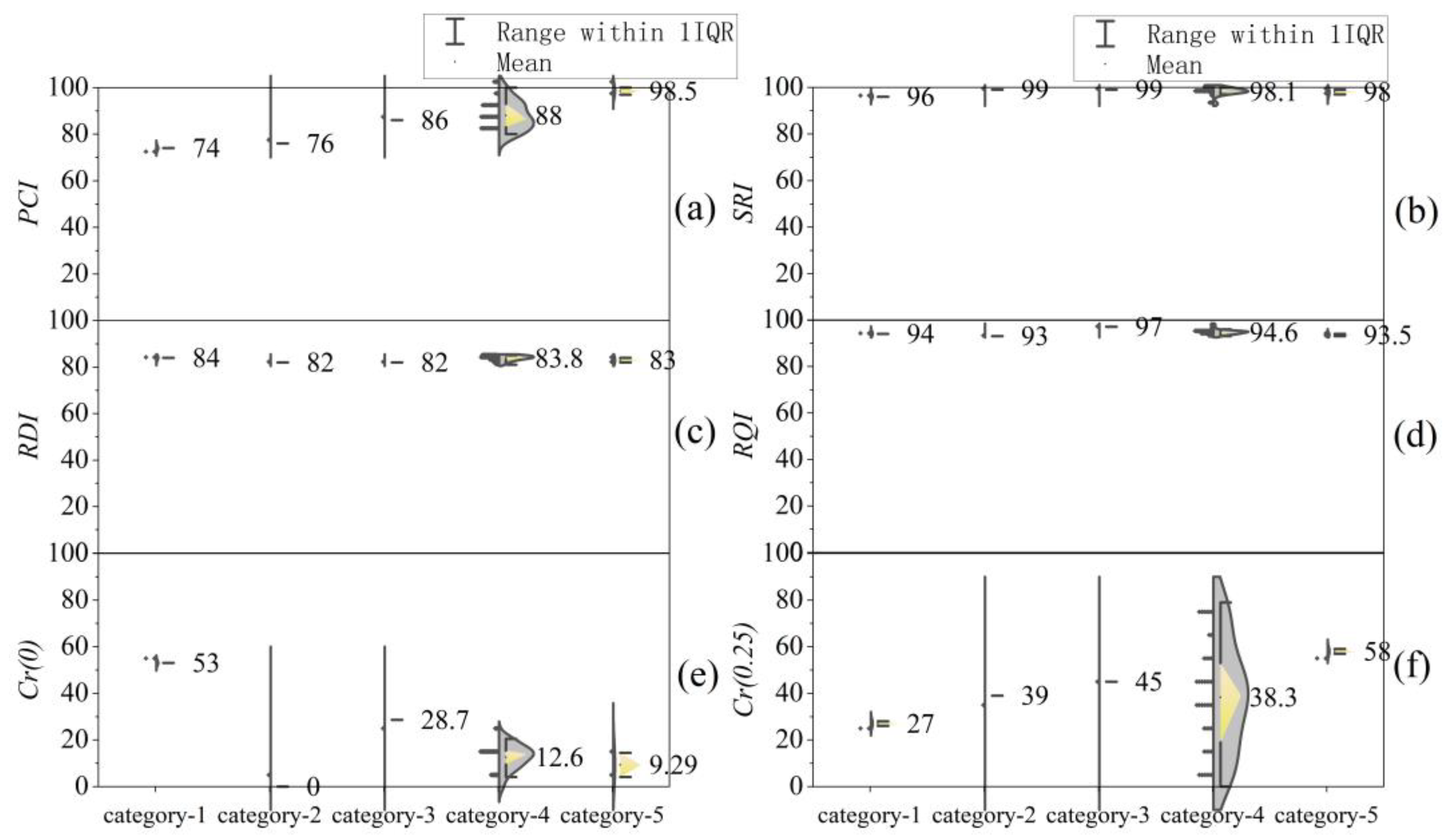
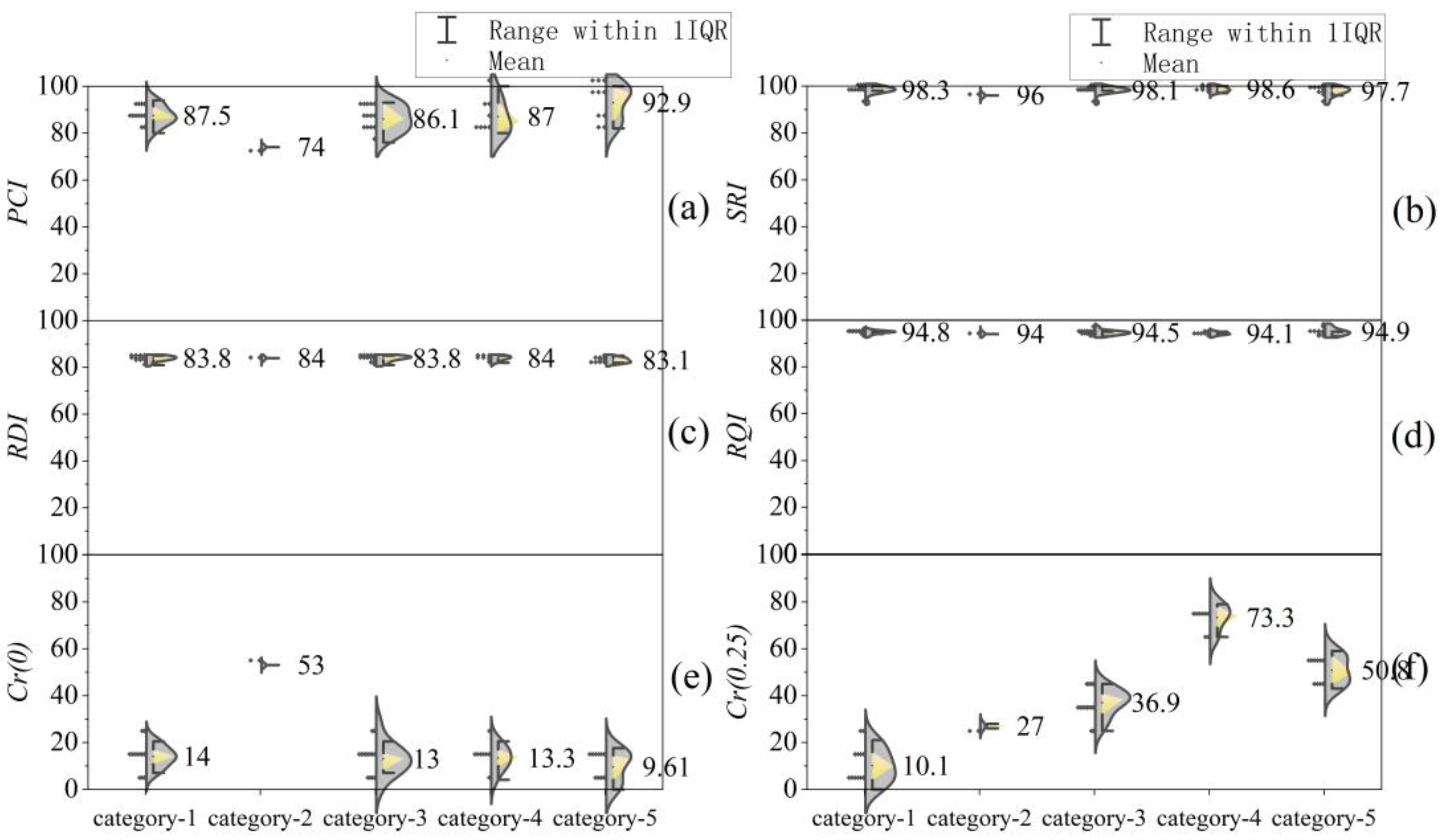
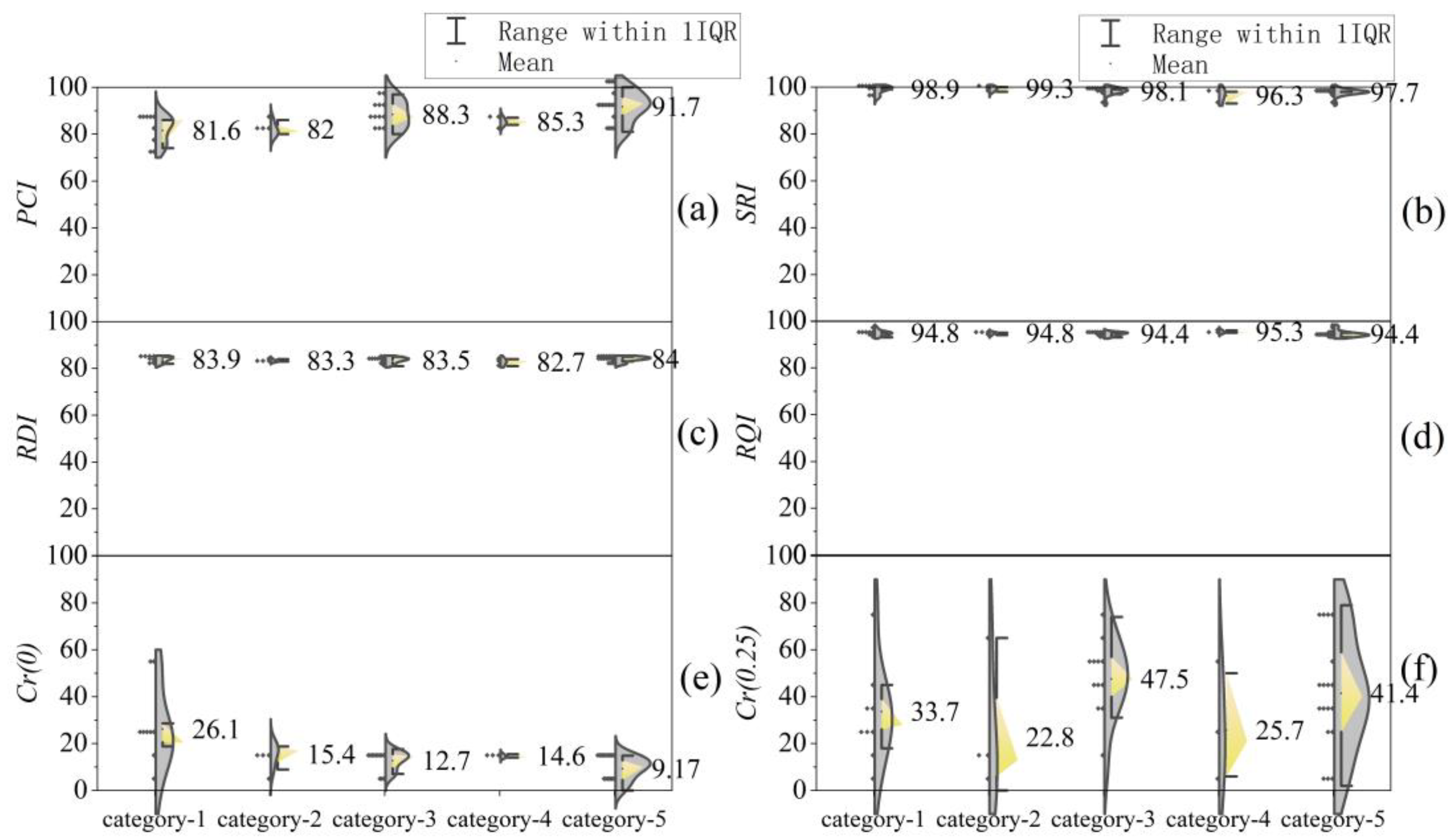
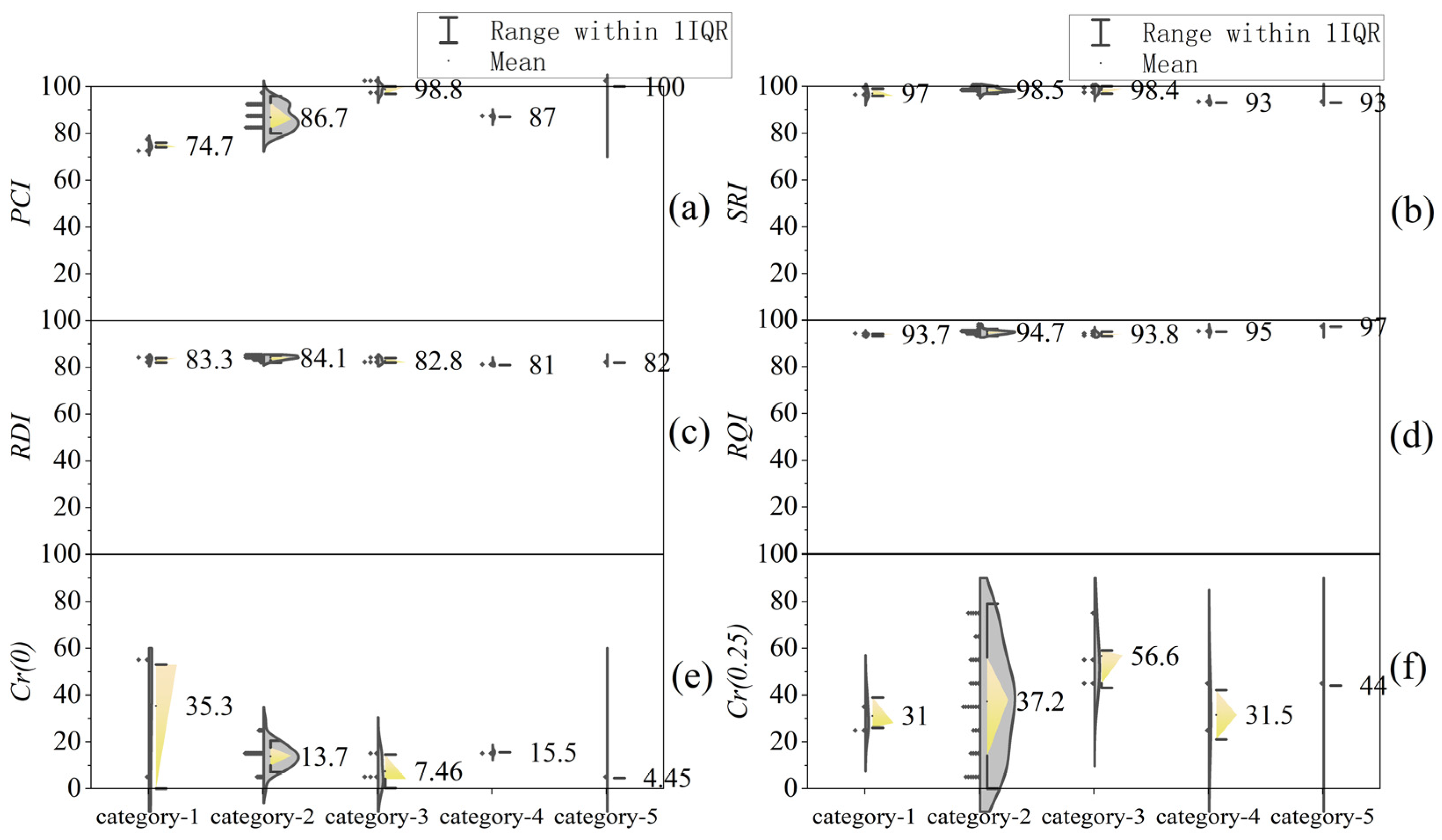
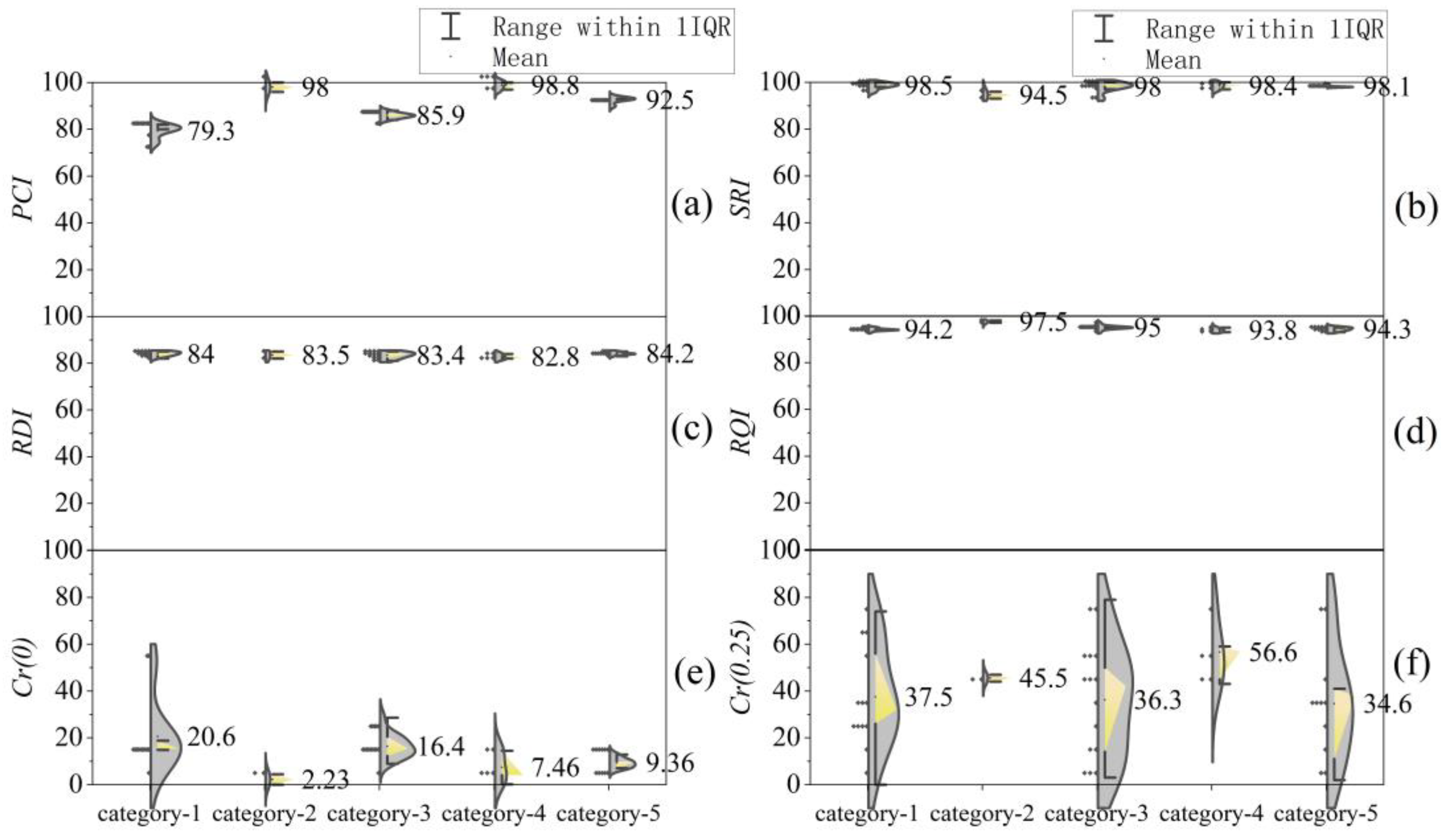
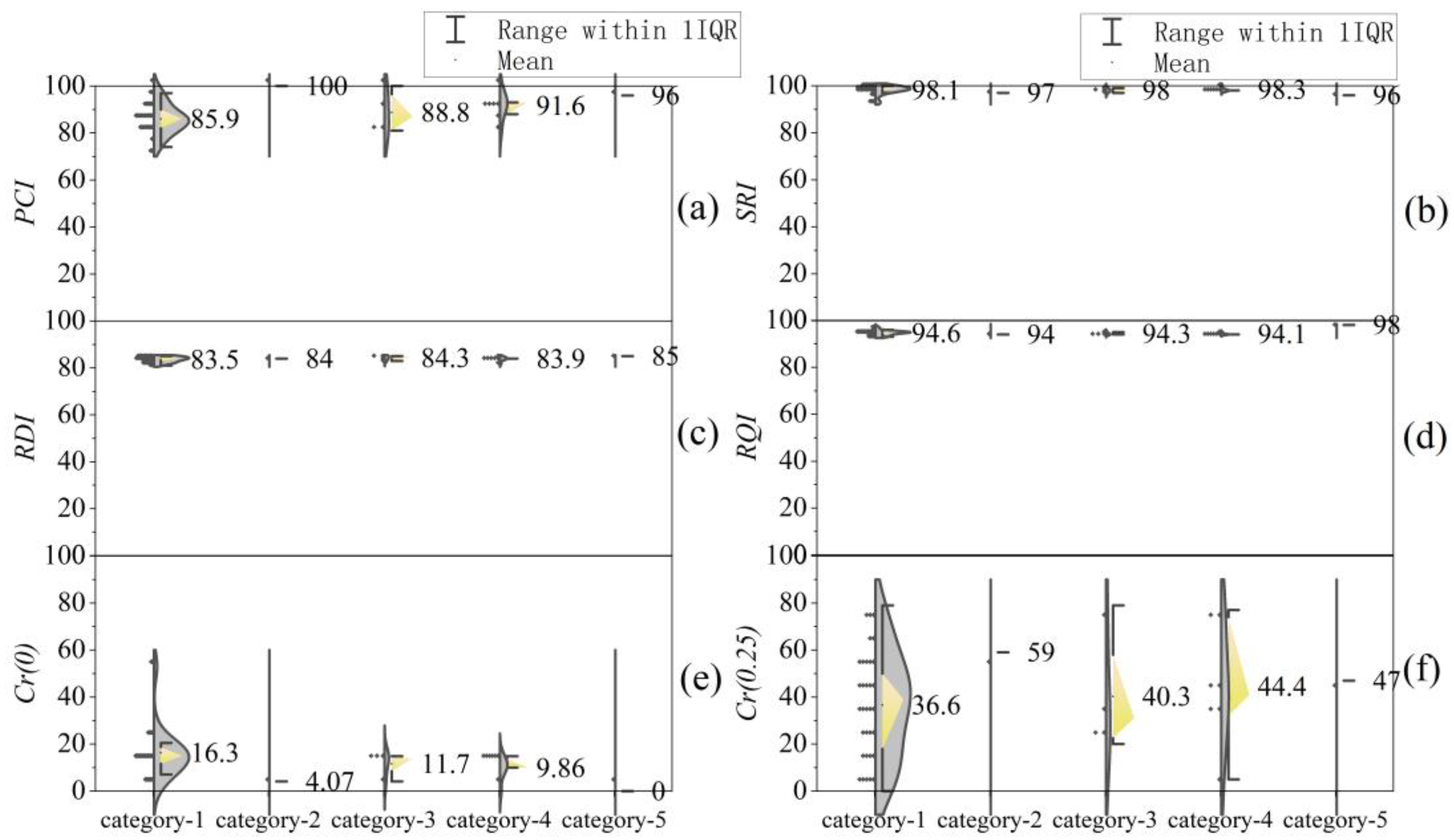
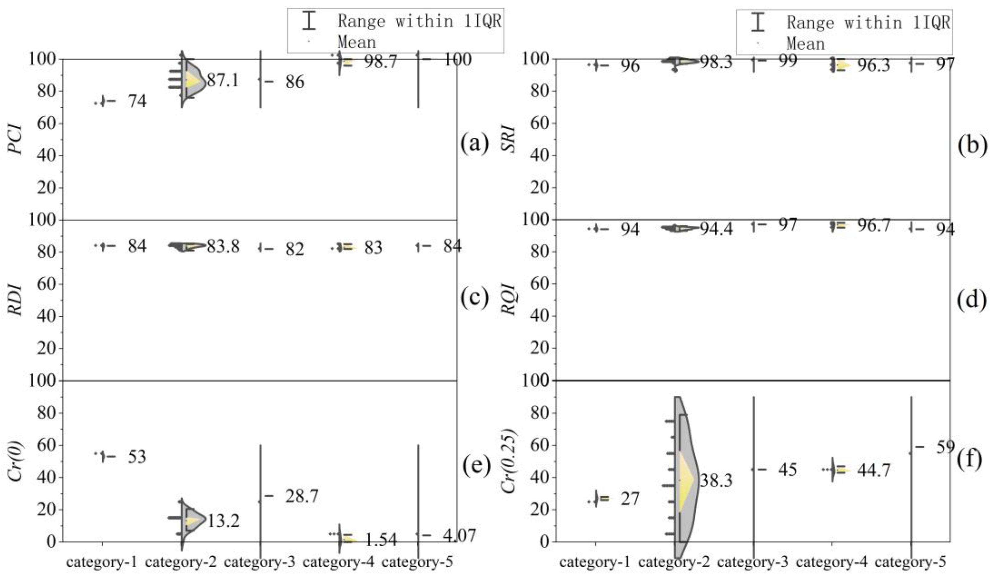
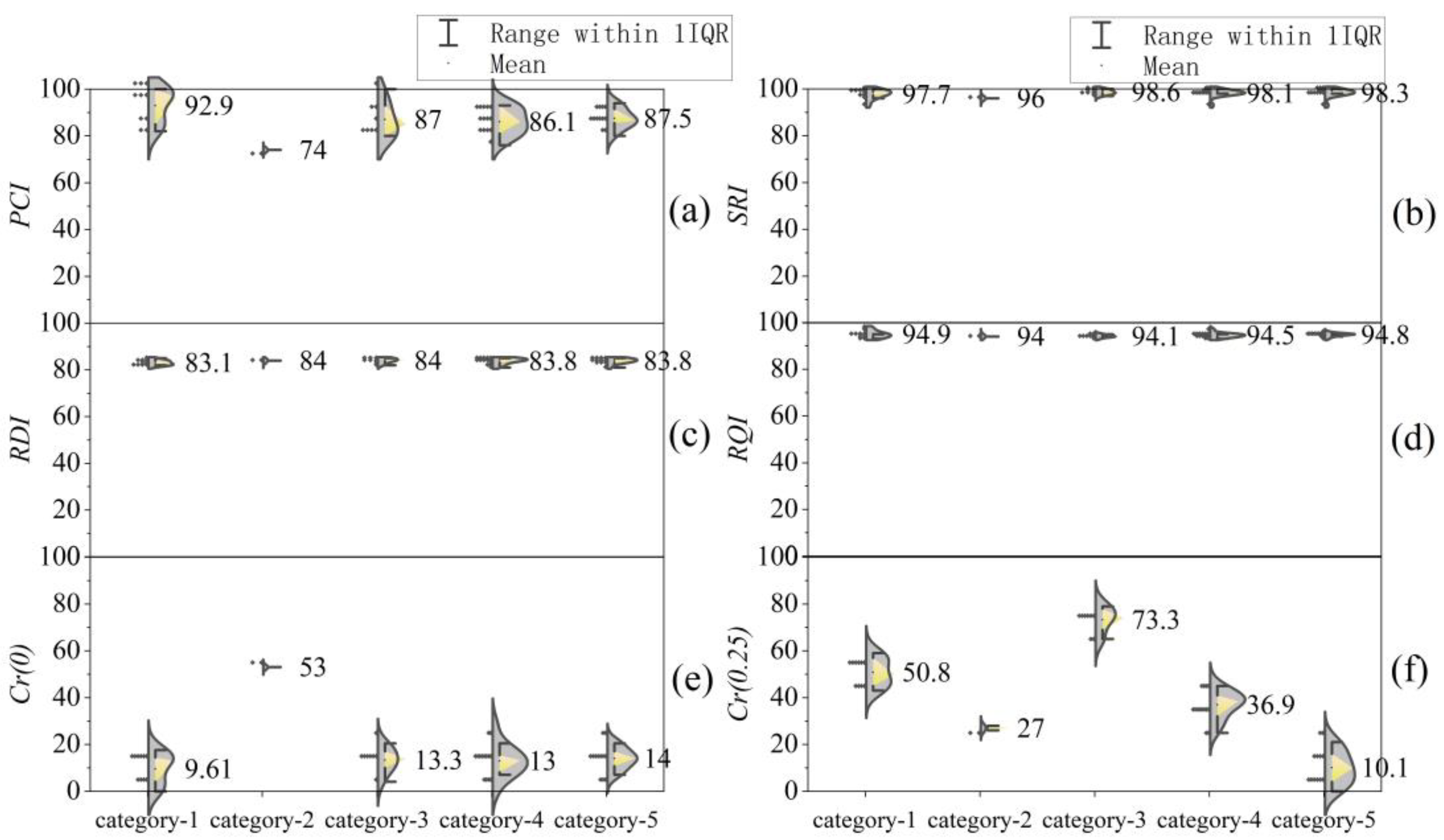
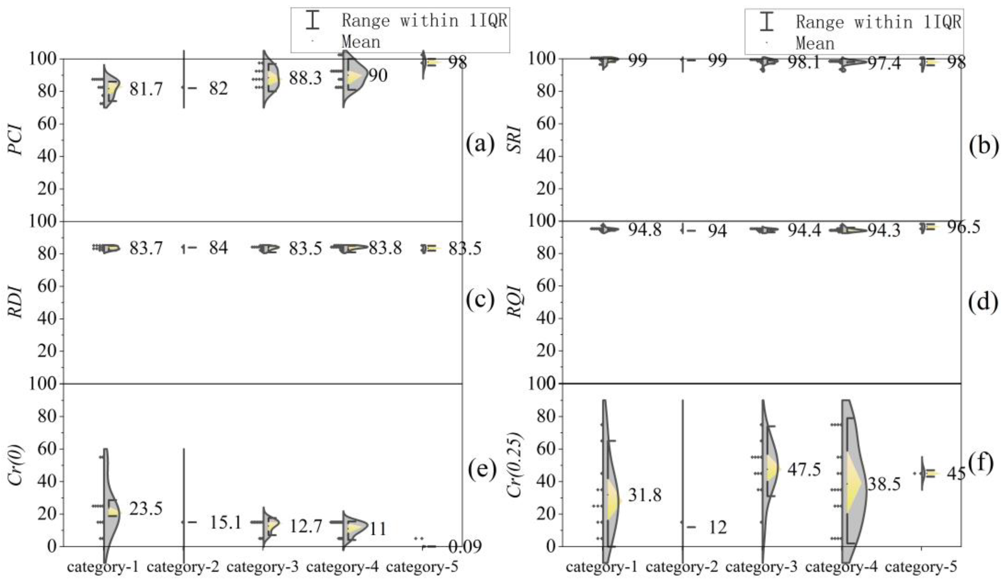
4.2. Analysis of Clustering Results

The systematic clustering, dynamic clustering and ordered clustering analysis methods mentioned in Section 2 were used to cluster the original variable data matrix $\left\{X_1,\dots ,X_6\right\}$, surface technical condition data $\left\{X_1,\dots ,X_4\right\}$ and principal components $\left\{Z_1,\dots ,Z_4\right\}$, respectively, in order to investigate the influence of the clustering methods, principal component analysis and pavement internal crack rate on the results of the section classification.

Considering that the asphalt pavement maintenance planning cycle generally lasts five years, the number of clusters in this was uniformly set to five. The results for the 46 unit sections classified for the GB1 project are shown in

Table 7. Clustering results for 46 unit sections for the GB1project.

Clustering Method		Category 1	Category 2	Category 3	Category 4	Category 5
Systematic clustering	X1 –X4	1–3	4–19, 22–24, 27–31, 33, 36–44, 46	20–21, 34–35, 45	25–26	32
	X1 –X6	1–2	3	4	5–19, 21–33, 35–46	20, 34
	Z1 –Z4	1–2	3, 5–31, 33, 35–44	4	32, 45–46	34
Dynamic clustering	X1 –X4	1–3, 9–11, 13–16, 37–39	32, 46	4–8, 12, 17–19, 25–28, 31, 40	20–21, 34–35, 45	22, 24, 29–30, 33, 36, 41–44
	X1 –X6	6, 8, 11–13, 23, 26–27, 29, 33, 36, 40	1–2	3–5, 9, 18, 22, 24–25, 30, 37–39, 41, 44	7, 10, 15–16, 31, 35, 42–43	14, 17, 19–21, 28, 32, 34, 45–46
	Z1 –Z4	14, 17, 19–21, 28, 32, 34, 45–46	1–2	7, 10, 15–16, 31, 35, 42–43	3–5, 9, 18, 22, 24–25, 30, 37–39, 41, 44	6, 8, 11–13, 23, 26–27, 29, 33, 36, 40
Ordered clustering	X1 –X4	1–33	34	35–38	39–45	46
	X1–X6	1–9	10–13	14–25	26–28	29–46
	Z1 –Z4	1–12	13	14–25	26–44	45–46

.

As shown in Table 7, there were significant differences in the classification results of the various clustering methods. The results using the principal components $\left\{Z_1,\dots ,Z_4\right\}$ and $\left\{X_1,\dots ,X_6\right\}$ had a relatively high degree of overlap, which side-by-side verified the ability of the PCA to retain information about the original data.

Box plots indicating the statistical distribution of each technical indicator for different combinations of clustered data and different clustering methods and principal component techniques are shown in Figure 2, Figure 3, Figure 4, Figure 5, Figure 6, Figure 7, Figure 8, Figure 9 and Figure 10. These figures show the mean value and the range of distribution for each technical indicator in each of the five categories. Using Figure 2 as an example, the means of $Cr\left(0\right)$ and $Cr\left(0.25\right)$ were relatively distinctly different, while the means of $PCI$, $SRI$, $RDI$ and $RQI$ were very similar. The graphs could reflect the variability of the results under the scheme using the data matrix $\left\{X_1,\dots ,X_6\right\}$ with the application of the hierarchical clustering method.

As shown by Figure 2, Figure 3, Figure 4, Figure 5, Figure 6, Figure 7, Figure 8, Figure 9 and Figure 10, the results obtained by the different clustering methods did not necessarily differ when analysing their individual specific indicators. In addition, when the ordered clustering method was utilized, the mean values and distribution ranges of the technical indicators obtained for each clustered sub-section were less differentiated, regardless of the type of clustered data used and regardless of whether the principal component method was used. When the hierarchical clustering method was used, the differentiation of indicator $PCI$ in the clustered sub-sections was better. When the dynamic clustering method was used, the differentiation of $Cr\left(0.25\right)$ in the clustered sub-sections was better. In terms of the selection of clustered data, when the clustered data did not contain $Cr\left(0\right)$ and $Cr\left(0.25\right)$, $Cr\left(0\right)$ and $Cr\left(0.25\right)$ also did not appear in the clustered results for indicators with high differentiation.

The ultimate goal of clustering is to classify the most similar unit sections into a particular sub-section. In order to more objectively compare the advantages and disadvantages of different clustering methods, a statistical ANOVA was conducted for the data for each technical index of the sub-sections classified by different clustering methods, and a p-value was used to characterise the significance of the differences between the data of each sub-section (see Figure 11). Statistically, the smaller the p-value, the more significant the differences between the data for each sub-section will be.

As can be seen from Figure 11, there was a genetic relationship between the clustering base data characteristics and the technical characteristics of the delineated sub-sections. When using $\left\{X_1,\dots ,X_6\right\}$ and $\left\{Z_1,\dots ,Z_4\right\}$, the p-values for $Cr\left(0.25\right)$ obtained by the dynamic and ordered clustering methods were significantly larger than those obtained by using $\left\{X_1,\dots ,X_4\right\}$. The sub-sections resulting from $\left\{X_1,\dots ,X_4\right\}$ did not reflect the differential characteristics of $Cr\left(0.25\right)$, which was related to the fact that the underlying data used for the clustering segments did not contain $Cr\left(0.25\right)$. $Cr\left(0\right)$ also exhibited similar characteristics, with the p-values from $\left\{X_1,\dots ,X_6\right\}$ and $\left\{Z_1,\dots ,Z_4\right\}$ being significantly smaller than that from $\left\{X_1,\dots ,X_4\right\}$, and this pattern held true for the systematic clustering approach as well. This result suggests that, when classifying asphalt pavements, if the difference in the technical characteristics of an aspect of the asphalt pavement is to be reflected in the classified section, it is necessary to include that technical indicator in the construction of the clustering data matrix, such as with $Cr\left(0\right)$ and $Cr\left(0.25\right)$ studied in this paper.

According to the results in Table 3, $PCI$ and $Cr\left(0\right)$ were the most significantly correlated, so they reflected essentially the same pattern of data. However, the p-values of the clustering results for indicators $SRI$, $RDI$ and $RQI$ did not reflect a similar pattern as for $PCI$, $Cr\left(0\right)$ and $Cr\left(0.25\right)$. In particular, for $\mathrm{S}\mathrm{R}\mathrm{I}$, the p-values of $\left\{X_1,\dots ,X_6\right\}$ and $\left\{Z_1,\dots ,Z_4\right\}$ were significantly greater for the systematic and dynamic clustering methods than that of $\left\{X_1,\dots ,X_4\right\}$, but the results were reversed when the ordered clustering method was used. For $RDI$, the ordered clustering method resulted in significantly larger p-values for $\left\{Z_1,\dots ,Z_4\right\}$ than for $\left\{X_1,\dots ,X_6\right\}$ and $\left\{X_1,\dots ,X_4\right\}$, while the systematic and dynamic clustering methods resulted in significantly larger p-values for $\left\{X_1,\dots ,X_6\right\}$ and $\left\{Z_1,\dots ,Z_4\right\}$ than that for $\left\{X_1,\dots ,X_4\right\}$. For $RQI$, dynamic and ordered clustering methods showed significantly larger p-values for $\left\{X_1,\dots ,X_6\right\}$ and $\left\{Z_1,\dots ,Z_4\right\}$ than for the segmentation results for $\left\{X_1,\dots ,X_4\right\}$.

In general, there were certain applicable relationships between the different clustering methods and the clustered data.

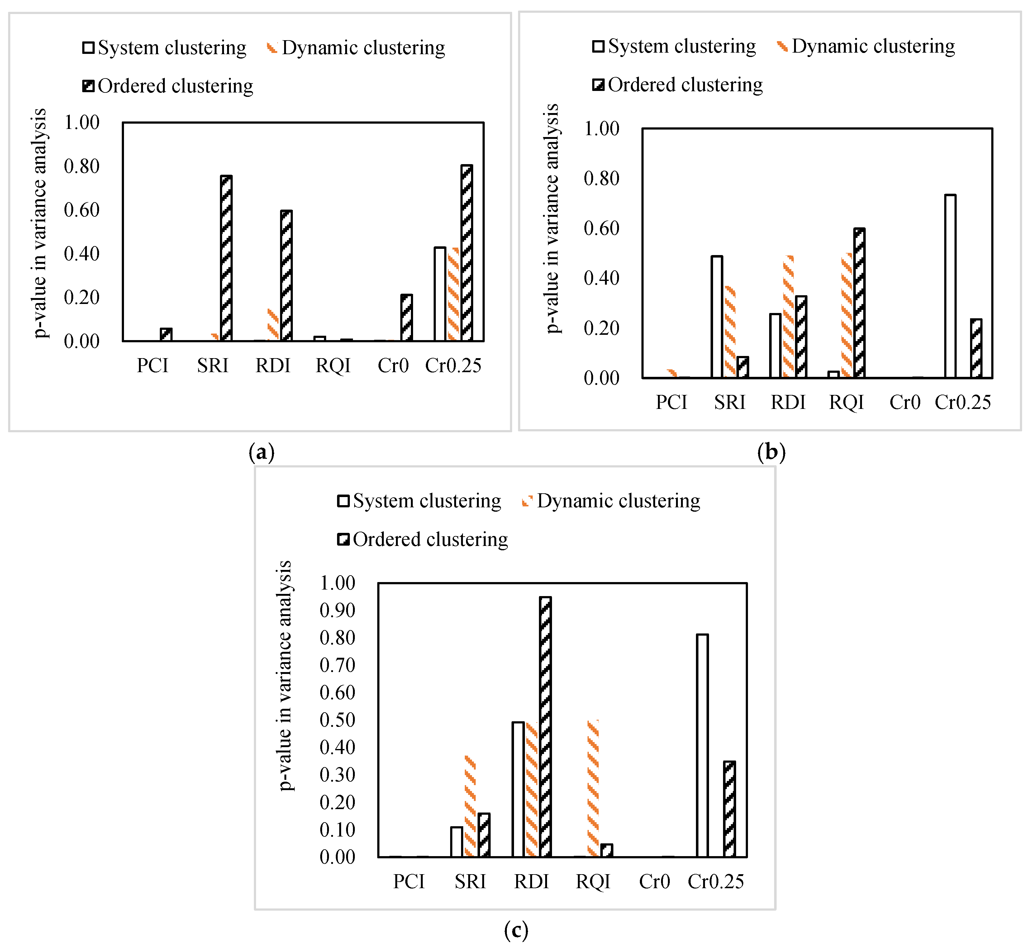
4.3. Applicability of Clustering Methods

In the practice of asphalt pavement maintenance and management, managers usually wish to design maintenance plans according to consecutive ordered segments, as this makes it more convenient and easier to allocate maintenance resources (which involve the transportation of construction materials, equipment and personnel, traffic organisation and other management issues), and consecutive segments are more conducive to mechanised operations and maintenance and repair quality assurance. Therefore, the ordered clustering method has been the more widely recommended method. However, as shown by Figure 11, although the ordered clustering method maximised the continuous and ordered merging of the different unit sections, the final clustering results did not guarantee that the technical characteristics of each sub-section were in a significantly different state after clustering. Five of the seven indicators (more than 71%) from the ordered clustering results in Figure 11a had higher p-value levels than in the systematic and dynamic clustering. The technical disadvantage of the ordered clustering method is that it tends to make it difficult to differentiate the maintenance plans for each sub-section, and it is not suitable for projects that require a high degree of refinement in the technical requirements of the maintenance plans. However, for projects that are limited by traffic volumes or other management factors, the ordered clustering method can be used.

Observing Figure 11, it can be seen that the p-value levels with the systematic clustering method were lower than 0.05 for all indicators except the indicator when clustering the segmentation of $\left\{X_1,\dots ,X_4\right\}$ (see Figure 11a). In addition, when applying the systematic clustering method, adding the internal crack rate to the data matrix caused significantly higher p-values for indicators $SRI$, $RDI$ and $Cr\left(0.25\right)$ for different sub-sections (see Figure 11a,b). Combining the functional indicators and the internal crack rate when classifying pavement sections using the systematic clustering method may have negative effects. Therefore, for projects that focus only on the surface functional indicators, a systematic clustering approach is advantageous.

The dynamic clustering method is suitable for projects that focus on the impact of the internal pavement condition on pavement maintenance needs. Adding the internal crack rate indicator resulted in significantly higher p-values for indicators $PCI$, $SRI$, $RDI$ and $RQI$ for different sub-sections but also significantly reduced the p-values for indicators $Cr\left(0\right)$ and $Cr\left(0.25\right)$, allowing the clustering to delineate sub-sections that could better reflect the differentiation of the internal disease characteristics of the asphalt pavements (see Figure 11a,b). The dynamic clustering method combined with principal component analysis could significantly improve the significance of the differences for the indicators of interest ($Cr\left(0\right)$ and $Cr\left(0.25\right)$) in the clustering results. It could also further reduce the p-values of the indicators not of interest ($PCI$, $SRI$, $RDI$ and $RQI)$ in the clustering results (see Figure 11b,c), effectively improving the segmentation of asphalt pavement maintenance sections.

5. Conclusions

To classify pavement maintenance sections, a clustering method based on 3D GPR and principal component analysis was proposed in this work. The effects of the clustering methods, principal component analysis and pavement internal crack rate on the classification results were investigated by analysing the significance of the variations in the classification results. The conclusions are as follows.

(1)

The characteristics of the cluster data and the technical characteristics of the subdivisions are genetically related. A clustering data matrix that takes into account internal cracking rates is essential in order to provide an effective means of classifying differences in asphalt pavement performance or maintenance requirements;

(2)

Classification results vary considerably between clustering methods and the choice of clustering method is related to pavement maintenance objectives. Ordered clustering is not suitable for projects requiring sophisticated maintenance plans, whereas it could be considered for traffic-limited projects. For projects focusing on surface functional indicators only, systematic clustering is advantageous, but combining functional and internal crack rates may be counterproductive. Dynamic clustering is suitable for projects focusing on internal distress effects;

(3)

Principal component analysis could reduce data matrix dimensionality by 33% and retain more than 84% of the information. The dynamic clustering method combined with the principal component analysis could significantly improve the significance of the differences for the indicators of interest in the clustering results, as well as the indicators not of interest, effectively improving the classification of asphalt pavement maintenance sections.

The limitations of this study were that limited data from one project were used for the analysis, but the data need to be more representative, and a more in-depth analysis will be conducted using data from multiple projects in the future. The application and validation of the asphalt pavement maintenance section classification method studied in this paper in maintenance science decision making will be followed up.

References

1. Peterson, J.C.; Bourgin, D.D.; Agrawal, M.; Reichman, D.; Griffiths, T.L. Using large-scale experiments and machine learning to discover theories of human decision-making. Science 2021, 372, 1209–1214. [Google Scholar] [CrossRef] [PubMed]
2. Davids, E.L. The Interaction between Basic Psychological Needs, Decision-Making and Life Goals among Emerging Adults in South Africa. Soc. Sci. 2022, 11, 316. [Google Scholar] [CrossRef]
3. Babashamsi, P.; Khahro, S.H.; Omar, H.A.; Al-Sabaeei, A.M.; Memon, A.M.; Milad, A.; Khan, M.I.; Sutanto, M.H.; Yusoff, N.I. Perspective of Life-Cycle Cost Analysis and Risk Assessment for Airport Pavement in Delaying Preventive Maintenance. Sustainability 2022, 14, 2905. [Google Scholar] [CrossRef]
4. Mousa, M.R.; Elseifi, M.A.; Zhang, Z.; Gaspard, K. Development of a Decision-Making Tool to Select Optimum Preventive Maintenance Treatments in a Hot and Humid Climate. Transp. Res. Rec. J. Transp. Res. Board 2020, 2674, 44–56. [Google Scholar] [CrossRef]
5. Miah, M.T.; Oh, E.; Chai, G.; Bell, P. An overview of the airport pavement management systems (APMS). Int. J. Pavement Res. Technol. 2021, 13, 581–590. [Google Scholar] [CrossRef]
6. Fani, A.; Golroo, A.; Mirhassani, S.A.; Gandomi, A.H. Pavement maintenance and rehabilitation planning optimisation under budget and pavement deterioration uncertainty. Int. J. Pavement Eng. 2020, 23, 414–424. [Google Scholar] [CrossRef]
7. Chen, W.; Zheng, M. Multi-objective optimization for pavement maintenance and rehabilitation decision-making: A critical review and future directions. Autom. Constr. 2021, 130, 103840. [Google Scholar] [CrossRef]
8. Mo T. JTG 5142-2019; Technical Specifications for Maintenance of HighwayAsphalt Pavement. China Communications Press: Beijing, China, 2019.
9. JTG H20-2007; Highway Performance Assessment Standards. Ministry of Transport of the People’s Republic of China: Beijing, China, 2008.
10. Anastasopoulos, P.C.; Mannering, F.L. Analysis of Pavement Overlay and Replacement Performance Using Random Parameters Hazard-Based Duration Models. J. Infrastruct. Syst. 2015, 21, 04014024. [Google Scholar] [CrossRef]
11. Cinar, Z.M.; Abdussalam Nuhu, A.; Zeeshan, Q.; Korhan, O.; Asmael, M.; Safaei, B. Machine Learning in Predictive Maintenance towards Sustainable Smart Manufacturing in Industry 4.0. Sustainability 2020, 12, 8211. [Google Scholar] [CrossRef]
12. Li, F.; Feng, J.; Li, Y.; Zhou, S. Introduction to the Pavement Preventive Maintenance Technology. Preventive Maintenance Technology for Asphalt Pavement; Springer Tracts on Transportation and Traffic; Springer: Berlin/Heidelberg, Germany, 2021; pp. 1–35. [Google Scholar]
13. Amarasiri, S.; Muhunthan, B. Evaluating the Effectiveness of Pavement Preventive-Maintenance Treatments in Mitigating Longitudinal Cracks in Wet-Freeze Climatic Zones. J. Transp. Eng. Part B Pavements 2020, 146, 04020014. [Google Scholar] [CrossRef]
14. Yamany, M.S.; Abraham, D.M. Hybrid Approach to Incorporate Preventive Maintenance Effectiveness into Probabilistic Pavement Performance Models. J. Transp. Eng. Part B Pavements 2021, 147, 04020077. [Google Scholar] [CrossRef]
15. Li, J.; Yin, G.; Wang, X.; Yan, W. Automated decision making in highway pavement preventive maintenance based on deep learning. Autom. Constr. 2022, 135, 104111. [Google Scholar] [CrossRef]
16. Hassan, M.U.; Steinnes, O.-M.H.; Gustafsson, E.G.; Løken, S.; Hameed, I.A. Predictive Maintenance of Norwegian Road Network Using Deep Learning Models. Sensors 2023, 23, 2935. [Google Scholar] [CrossRef] [PubMed]
17. Nautiyal, A.; Sharma, S. Cost-Optimized Approach for Pavement Maintenance Planning of Low Volume Rural Roads: A Case Study in Himalayan Region. Int. J. Pavement Res. Technol. 2022, 1–18. [Google Scholar] [CrossRef]
18. Liang, X.; Yu, X.; Chen, C.; Jin, Y.; Huang, J. Automatic Classification of Pavement Distress Using 3D Ground-Penetrating Radar and Deep Convolutional Neural Network. IEEE Trans. Intell. Transp. Syst. 2022, 23, 22269–22277. [Google Scholar] [CrossRef]
19. Xiong, C.; Yu, J.; Zhang, X. Use of NDT systems to investigate pavement reconstruction needs and improve maintenance treatment decision-making. Int. J. Pavement Eng. 2021, 1–15. [Google Scholar] [CrossRef]
20. Liu, Z.; Wu, W.; Gu, X.; Li, S.; Wang, L.; Zhang, T. Application of Combining YOLO Models and 3D GPR Images in Road Detection and Maintenance. Remote Sens. 2021, 13, 1081. [Google Scholar] [CrossRef]
21. Hong, X.; Tan, W.; Xiong, C.; Qiu, Z.; Yu, J.; Wang, D.; Wei, X.; Li, W.; Wang, Z. A Fast and Non-Destructive Prediction Model for Remaining Life of Rigid Pavement with or without Asphalt Overlay. Buildings 2022, 12, 868. [Google Scholar] [CrossRef]
22. Di Mascio, P.; Moretti, L. Implementation of a pavement management system for maintenance and rehabilitation of airport surfaces. Case Stud. Constr. Mater. 2019, 11, e00251. [Google Scholar] [CrossRef]
23. Gkyrtis, K.; Plati, C.; Loizos, A. Mechanistic Analysis of Asphalt Pavements in Support of Pavement Preservation Decision-Making. Infrastructures 2022, 7, 61. [Google Scholar] [CrossRef]
24. Nautiyal, A.; Sharma, S. Methods and factors of prioritizing roads for maintenance: A review for sustainable flexible pavement maintenance program. Innov. Infrastruct. Solut. 2022, 7, 190. [Google Scholar] [CrossRef]
25. Elmansouri, O.; Alossta, A.; Badi, I. Pavement Condition Assessment Using Pavement Condition Index and Multi-Criteria Decision-Making Model. Mechatronics Intell. Transp. Syst. 2022, 1, 57–68. [Google Scholar] [CrossRef]
26. Fang, N.; Chang, H.; Hu, S.; Li, H.; Meng, Q. Climate zoning of asphalt pavement based on spatial interpolation and Fuzzy C-Means algorithm. Int. J. Pavement Eng. 2022, 1–14. [Google Scholar] [CrossRef]
27. Milad, A.A.; Adwan, I.; Majeed, S.A.; Memon, Z.A.; Bilema, M.; Omar, H.A.; Abdolrasol, M.G.M.; Usman, A.; Yusoff, N.I.M. Development of a Hybrid Machine Learning Model for Asphalt Pavement Temperature Prediction. IEEE Access 2021, 9, 158041–158056. [Google Scholar] [CrossRef]
28. Han, C.; Ma, T.; Chen, S. Asphalt pavement maintenance plans intelligent decision model based on reinforcement learning algorithm. Constr. Build. Mater. 2021, 299, 124278. [Google Scholar] [CrossRef]
29. Ezugwu, A.E.; Ikotun, A.M.; Oyelade, O.O.; Abualigah, L.; Agushaka, J.O.; Eke, C.I.; Akinyelu, A.A. A comprehensive survey of clustering algorithms: State-of-the-art machine learning applications, taxonomy, challenges, and future research prospects. Eng. Appl. Artif. Intell. 2022, 110, 104743. [Google Scholar] [CrossRef]
30. Dalmaijer, E.S.; Nord, C.L.; Astle, D.E. Statistical power for cluster analysis. BMC Bioinform. 2022, 23, 205. [Google Scholar] [CrossRef] [PubMed]
31. Li, T.; Rezaeipanah, A.; El Din, E.M.T. An ensemble agglomerative hierarchical clustering algorithm based on clusters clustering technique and the novel similarity measurement. J. King Saud Univ.-Comput. Inf. Sci. 2022, 34, 3828–3842. [Google Scholar] [CrossRef]
32. Habib, A.; Akram, M.; Kahraman, C. Minimum spanning tree hierarchical clustering algorithm: A new Pythagorean fuzzy similarity measure for the analysis of functional brain networks. Expert Syst. Appl. 2022, 201, 117016. [Google Scholar] [CrossRef]
33. Ashari, I.F.; Banjarnahor, R.; Farida, D.R.; Aisyah, S.P.; Dewi, A.P.; Humaya, N. Application of Data Mining with the K-Means Clustering Method and Davies Bouldin Index for Grouping IMDB Movies. J. Appl. Inform. Comput. 2022, 6, 7–15. [Google Scholar] [CrossRef]
34. Nie, F.; Li, Z.; Wang, R.; Li, X. An Effective and Efficient Algorithm for K-Means Clustering with New Formulation. IEEE Trans. Knowl. Data Eng. 2022, 35, 3433–3443. [Google Scholar] [CrossRef]
35. Xia, J.; Ying, H.; Huang, Y. Application of ordered aggregation optimal partition method in pavement condition evaluation. In Frontier Research: Road and Traffic Engineering; CRC Press: Boca Raton, FL, USA, 2022; pp. 700–706. [Google Scholar]
36. Tang, H.; Wang, Y.; Jia, K. Unsupervised domain adaptation via distilled discriminative clustering. Pattern Recognit. 2022, 127, 108638. [Google Scholar] [CrossRef]
37. JTG E60-2008; Field Test Methods of Highway Subgrade and Pavement. Ministry of Transport of the People’s Republic of China: Beijing, China, 2008.
38. Liu, Z.; Gu, X.; Chen, J.; Wang, D.; Chen, Y.; Wang, L. Automatic recognition of pavement cracks from combined GPR B-scan and C-scan images using multiscale feature fusion deep neural networks. Autom. Constr. 2023, 146, 104698. [Google Scholar] [CrossRef]
39. Wang, S.; Leng, Z.; Sui, X. Detectability of concealed cracks in the asphalt pavement layer using air-coupled ground-penetrating radar. Measurement 2023, 208, 112427. [Google Scholar] [CrossRef]
40. Liu, Z.; Gu, X. Performance evaluation of full-scale accelerated pavement using NDT and laboratory tests: A case study in Jiangsu, China. Case Stud. Constr. Mater. 2023, 18, e02083. [Google Scholar] [CrossRef]
41. Xiong, C.; Yu, J.; Zhang, X.; Korolev, E.; Svetlana, S.; Chen, B.; Chen, F.; Yang, E. Modulus backcalculation methodology based on full-scale testing road and its rationality and feasibility analysis. Int. J. Pavement Eng. 2022, 1–13. [Google Scholar] [CrossRef]
42. Burstyn, I. Principal component analysis is a powerful instrument in occupational hygiene inquiries. Ann. Occup. Hyg. 2004, 48, 655–661. [Google Scholar] [CrossRef] [PubMed] [Green Version]
43. Vidal-Alaball, J.; Mateo, G.F.; Domingo, J.L.G.; Gomez, X.M.; Valmaña, G.S.; Ruiz-Comellas, A.; Seguí, F.L.; Cuyàs, F.G. Validation of a Short Questionnaire to Assess Healthcare Professionals’ Perceptions of Asynchronous Telemedicine Services: The Catalan Version of the Health Optimum Telemedicine Acceptance Questionnaire. Int. J. Environ. Res. Public Health 2020, 17, 2202. [Google Scholar] [CrossRef] [Green Version]
Figure 1. Three-dimensional (3D) GPR detection and analysis: (a) 3D GPR detection; (b) represented result from 3D-Radar Examiner 3.5.
Buildings 13 01752 g001
Figure 2. Distribution of the different technical indicators of the classification results using data matrix X 1 , , X 6 with the application of the hierarchical clustering method: (a) P C I ; (b) S R I ; (c) R D I ; (d) R Q I ; (e) C r ( 0 ) ; (f) C r ( 0.25 ) .
Buildings 13 01752 g002
Figure 3. Distribution of the different technical indicators of the classification results using data matrix X 1 , , X 6 with the application of the dynamic clustering method: (a) P C I ; (b) S R I ; (c) R D I ; (d) R Q I ; (e) C r ( 0 ) ; (f) C r ( 0.25 ) .
Buildings 13 01752 g003
Figure 4. Distribution of the different technical indicators of the classification results using data matrix X 1 , , X 6 with the application of the ordered clustering method: (a) P C I ; (b) S R I ; (c) R D I ; (d) R Q I ; (e) C r ( 0 ) ; (f) C r ( 0.25 ) .
Buildings 13 01752 g004
Figure 5. Distribution of the different technical indicators of the classification results using data matrix X 1 , , X 4 with the application of the hierarchical clustering method: (a) P C I ; (b) S R I ; (c) R D I ; (d) R Q I ; (e) C r ( 0 ) ; (f) C r ( 0.25 ) .
Buildings 13 01752 g005
Figure 6. Distribution of the different technical indicators of the classification results using data matrix X 1 , , X 4 with the application of the dynamic clustering method: (a) P C I ; (b) S R I ; (c) R D I ; (d) R Q I ; (e) C r ( 0 ) ; (f) C r ( 0.25 ) .
Buildings 13 01752 g006
Figure 7. Distribution of the different technical indicators of the classification results using data matrix X 1 , , X 4 with the application of the ordered clustering method: (a) P C I ; (b) S R I ; (c) R D I ; (d) R Q I ; (e) C r ( 0 ) ; (f) C r ( 0.25 ) .
Buildings 13 01752 g007
Figure 8. Distribution of the different technical indicators of the classification results using data matrix Z 1 , , Z 4 with the application of the hierarchical clustering method and PCA: (a) P C I ; (b) S R I ; (c) R D I ; (d) R Q I ; (e) C r ( 0 ) ; (f) C r ( 0.25 ) .
Buildings 13 01752 g008
Figure 9. Distribution of the different technical indicators of the classification results using data matrix Z 1 , , Z 4 with the application of the dynamic clustering method and PCA: (a) P C I ; (b) S R I ; (c) R D I ; (d) R Q I ; (e) C r ( 0 ) ; (f) C r ( 0.25 ) .
Buildings 13 01752 g009
Figure 10. Distribution of the different technical indicators of the classification results using data matrix Z 1 , , Z 4 with the application of the ordered clustering method and PCA: (a) P C I ; (b) S R I ; (c) R D I ; (d) R Q I ; (e) C r ( 0 ) ; (f) C r ( 0.25 ) .
Buildings 13 01752 g010
Figure 11. Significance of the differences in the results obtained with different clustering data by different clustering methods: (a) using data for X1X4; (b) using data for X1X6; (c) using data for Z1Z4.
Buildings 13 01752 g011