Development of a Joint Penalty Signal for Building Energy Flexibility in Operation with Power Grids: Analysis and Case Study

Abstract

Electricity generation from renewable energy reduces greenhouse gas emissions and, in the long term, the cost of electricity in power grids. However, there is currently no strong positive correlation between greenhouse gas intensity and electricity spot prices in Germany, despite increasing renewable energy penetration. Therefore, energy flexibility programs that rely on demand response may not be fully effective in reducing carbon emissions unless the energy market aligns consistently with carbon emission factors. To address this issue, we propose a model for joint signals consisting of power grid climate gas intensity and price signals that can achieve both environmental and economic benefits for building energy flexibility applications. Next, to assess the maximum possible flexibility hours from the grid side, we explore penalty signal threshold limits with daily and biweekly aggregation. Using a case study, we analyze energy flexibility with joint signals to explore their effect on greenhouse gas emissions and building operation cost. Our results suggest that joint signals can be more effective than a single type of signal in promoting energy flexibility.

1. Introduction

The European Commission addresses the climate crisis and intends to decrease the current greenhouse gas (GHG) emissions by at least 55% by 2030 compared to 1990 levels [1]. Looking further ahead, the Commission aims to achieve a further reduction of 55% in 2050 compared to 2030 [2]. Germany, which has high GHG emissions per capita compared to other EU countries and the global average, aims to reduce GHG emissions by 80–95% by 2050 compared to 1990 levels [3]. The country’s target for 2040 is a minimum reduction of 88%, with the goal of achieving GHG neutrality by 2045 [4]. On this path, Germany defines limits for the annual climate gas emissions by sectors and an annual control mechanism. To achieve the climate action goals, dissemination of renewable energy systems and energy efficiency investments are positive measures, hence heating systems based on renewable energy sources will be funded. The integration of renewable energy systems (RES) into the power supply is critical on the path to these targets. RES have intermittent form, coming from the variations in solar radiation and wind strength, which can result in variable electricity generation and fluctuating energy supply [5,6]. These changes over time within the power grid create stability issues [7].

National (Transmission) grids are responsible for transmitting electricity over long distances from large power plants to various regions of a country [8]. On the other hand, local (distribution) power grids distribute electricity from the national grid to homes and businesses in a specific area. The national and local power grids are different in design, function, and operational requirements due to the differences in the scale of their operation and the distances they cover [9]. As a result, electricity prices can vary between these grids due to factors such as generation costs, transmission costs, distribution costs [10,11], and stability issues. Moreover, electricity prices are influenced by the generation mix of electricity sources, which can vary between national and local power grids. Nevertheless, due to the cost reduction of RES technologies and the increasing cost of electricity generation by nonrenewable sources, RES is expected to contribute more significantly to the power grid globally [12].

Increasing electricity production from RES exposes energy providers to challenges in balancing supply and demand efficiently and economically [5]. To ensure efficient allocation of renewable and conventional energy, markets that allow for the trading of new information are crucial [13]. Increasing the flexibility and responsiveness of short-term wholesale markets to accommodate the growing share of renewable energy is suggested by the European Commission [14]. This proposes empowering consumers to participate in electricity markets by providing them with smart meters and dynamic retail tariffs that reflect changing wholesale prices, enabling them to make informed decisions about energy consumption [15]. To address this issue, energy flexibility in buildings as part of demand response management can be used to optimize the load in the power grid [5] based on various external factors such as power grid demand, energy price signal and CO_2eq. intensity.

Exploiting the potential of demand response has become an area of growing interest [16]. Demand response involves actions on the demand side by reacting to conditions in the power grid, providing an opportunity to reduce operating costs and GHG emissions [17]. However, the impact of demand–response programs on CO₂ emissions is often inaccurately assessed using dynamic power grid intensity [18]. The dynamic power grid intensity (CO_2eq. intensity) refers to the amount of CO₂ emissions released in the generation of one unit of electricity per hour. The marginal emissions factor based on specific generators’ CO₂ intensity provides a more accurate estimate of actual reductions rather than grid-average electricity [19]. The merit order dilemma, which refers to the preference for cheaper, more carbon-intensive technologies in the electricity generation process due to their low marginal costs, is often ignored [20]. Since accurately calculating marginal emissions at a given time is complex, identifying marginal generators and isolating their emissions can be challenging [21]. As a result, load shifting through demand–response programs cannot fully exploit the potential for carbon reduction unless the merit order of the energy market is correlated with carbon emission factors [20]. However, due to the mentioned complications, the CO_2eq. intensity signal based on average electricity emission factors are used conventionally in the present applications. In other words, the electricity spot price from the energy market and the commonly used CO_2eq. intensity value are not always positively correlated, which raises concerns about the optimizing method for both economic and environmental benefits in energy flexibility applications. Although energy storage can facilitate decarbonisation by boosting renewable energy integration in the long run, its effectiveness in reducing GHG emissions in the short term hinges on factors such as the storage technology used and its operational management [22].

The purpose of this paper is to develop a joint signal of price and CO_2eq. intensity and use it as a penalty signal for energy flexibility applications in buildings that achieves both environmental and economic savings. Modelling such a signal is a critical issue in building–grid studies to avoid one type of prominent saving since these signals are not always positively correlated. In the literature, there are various studies discussing the price and CO_2eq. intensity as a penalty signal to exploit the energy flexibility but, not much attention has been given to the joint influence of these signals and existing research with this focus is limited. One study [23] investigated the joint impact of both price and CO₂ signals in demand–response programmes using Markov–chain load models. Another study [24] conducted a tradeoff analysis between CO₂ emissions and electricity cost achieving both economic and environmental benefits by utilizing various schedules. [25] examined the combined impact of price and CO₂ emissions in demand response programmes and formulated an optimal control model to reduce energy cost and carbon emissions for five households in South Africa by mixed integer nonlinear programming. Similarly, [26] used mixed integer linear programming for an optimisation model to jointly minimize electricity costs and CO₂ emissions through an optimisation model for home energy management, achieving lower total cost, CO₂ emissions cost, and peak demand shaving. [27] used a mixed integer linear programming model with the ε-constraint method and Pareto curves to examine coordinated scheduling, which resulted in reduced cost and CO₂ emissions. A pilot study to evaluate the influence of real-time price visualisation on electricity consumption, electricity costs, and CO₂ emissions was performed [28]. Since there was a negative correlation between electricity price and CO_2eq. intensity in the Swedish electricity market in the period studied, the load shifting results showed a reduction in electricity costs while CO₂ emissions raised.

In this context, this paper introduces two joint penalty signals—concurrence penalty signal and combined penalty signal—and analyses their effectiveness when applied with threshold levels that determine the start of energy flexibility. To achieve this goal, the paper addresses the following research questions:

• What are the main drivers of the CO_2eq. intensity in the German power grid?

The power grid CO_2eq. intensity development is discussed in relation to the electricity spot price and energy flow.

2.

How does the observation interval affect the definition of penalty signal thresholds?

The paper analyses the upper and lower thresholds for CO_2eq intensity and electricity spot price and evaluates the flexibility operation under different observation intervals, such as daily and biweekly, for the heating season. Daily and biweekly observation times refer to the time intervals at which the penalty signals are monitored and used to determine the energy flexibility thresholds.

3.

What is the impact of joint penalty signals?

The penalty-unaware status of a case building is compared to different penalty-aware cases using four penalty signals, CO_2eq. intensity, electricity spot price (before tax), and two joint signals (concurrence and combined). Their effect on building performance metrics is discussed.

After this introduction (Section 1), this paper is structured as follows: Section 2 shows the calculation methodology of power grid CO_2eq. intensity, the threshold calculation of penalty signals and the methods to form the concurrence and combined penalty signals based on CO_2eq. intensity and price signals. Section 3 presents the factors influencing the power grid CO_2eq. intensity and its relationship with price signal. Additionally, the impact of the different observation intervals on the definition of the penalty signal thresholds is presented. In Section 4, the calculated thresholds are applied in a case study with the described penalty signals, and the result of the simulation results are illustrated. Section 5 discusses the implications of these findings and the analysis. Section 6 concludes the study.

2. Methodology

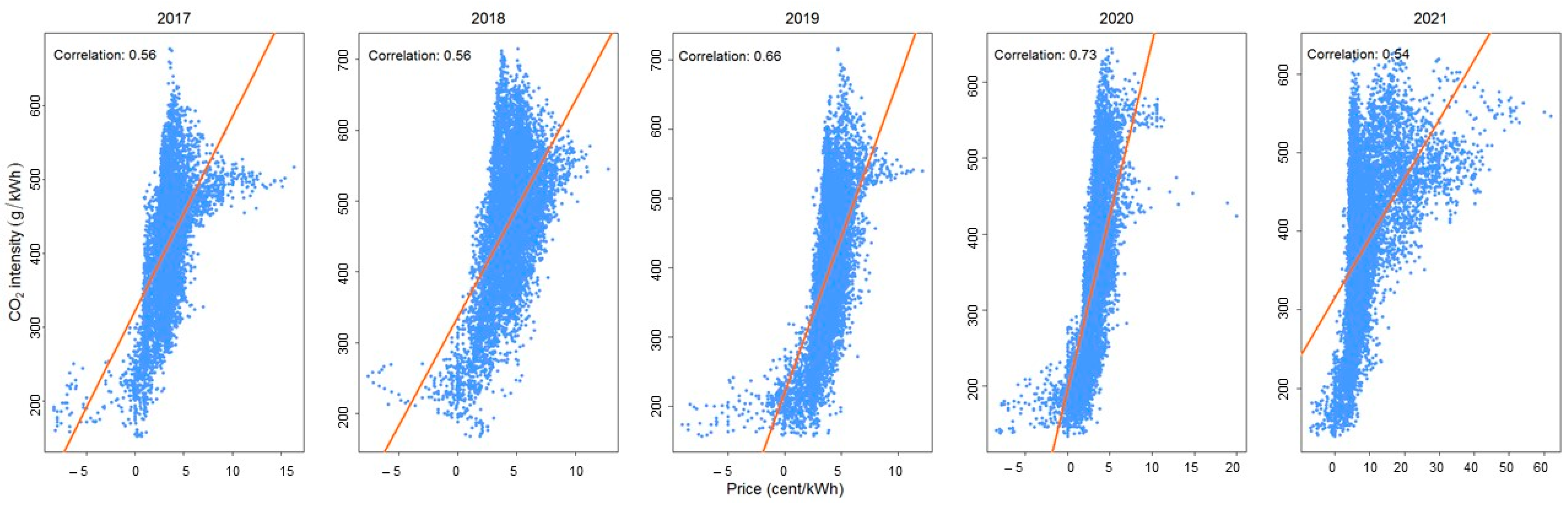
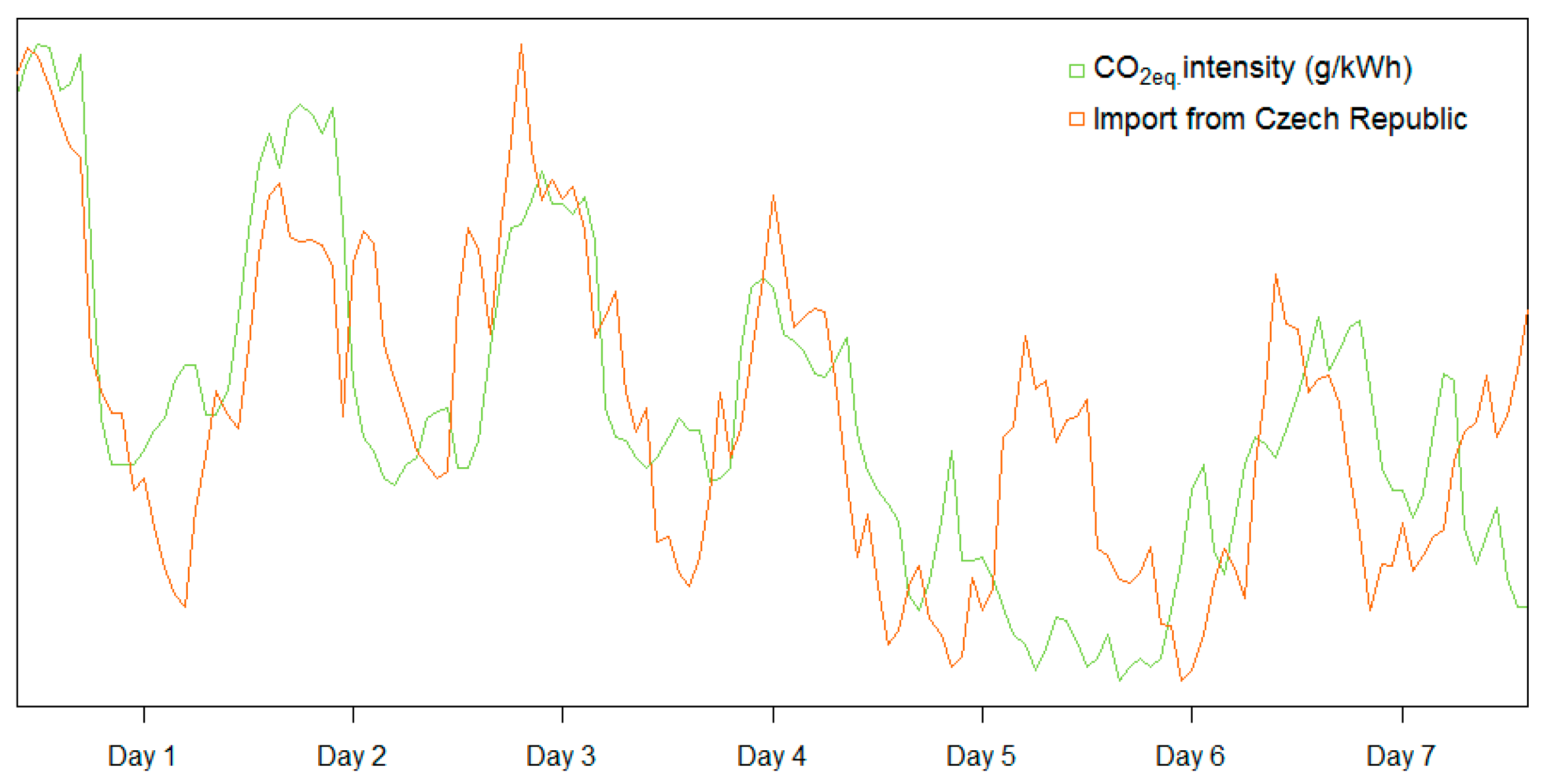
2.1. Dynamic CO_2eq. Intensity Calculation

The dynamic CO_2eq. intensity calculation data was collected from ENTSO-e [29], which provides free access to electricity production data and the energy flow information between countries with a time step of 15 or 60 min. The CO₂ emission factors for electricity production technologies are accessible from various resources. In Germany, the grid electricity is generated by 17 different technologies as shown in

Table 1. Climate gas emissions of various electricity generation technologies in Germany. Climate gases are expressed in CO₂ equivalents (Data source: [30].)

Electricity Production Technology	CO2 Coefficient (gCO2eq./kWh)
Biomass	70
Fossil brown coal/lignite	1054
Fossil coal-derived gas	433
Fossil gas	433
Fossil hard coal	873
Fossil oil	841
Geothermal	183
Hydro pumped storage-aggregated	14
Hydro run-of-river and poundage	3
Hydro water reservoir	14
Solar	67
Waste	342
Wind offshore	6
Wind onshore	10
Nuclear	68
Other	45
Other renewable	45

.

The production data and the energy flow between countries were obtained for the years 2017–2021, with the interconnected countries for energy flow varying by year.

Table 2. The CO_2eq. intensity of interconnected countries between 2017 and 2021 [31,32,33,34,35].

Country	CO2eq. Intensity (gCO2eq./kWh)
	2017	2018	2019	2020	2021
Austria	103	100	92	82	82
Belgium	-	-	174	161	140
Czech Republic	472	465	433	437	403
Denmark	179	193	123	109	155
France	69	58	56	51	58
Germany	413	404	344	311	349
Luxembourg	64	65	73	59	55
Netherlands	460	440	392	328	325
Norway	-	-	-	32	27
Poland	778	784	719	710	736
Sweden	10	11	10	9	10
Switzerland	35	35	35	35	35

presents the yearly average CO₂ emission coefficients of the connected countries. These data were only used as input for the emission calculation resulting from energy trade.

The CO_2eq. intensity in the power grid was influenced by five main factors, including the CO₂ emission coefficient of production technologies (Table 1), the share of technologies in use (from ENTSO-e platform with 60 min data resolution), the CO₂ emission coefficient of imported electricity based on countries (Table 2), and the amount of exported and imported electricity (ENTSO-e). Total CO₂ emissions coming from the production technologies were calculated using the electricity production amount and CO₂ emission coefficients from Table 1 by Equation (1). The average CO₂ emission coefficient of the import countries was used with the amount of imported electricity to calculate the total CO₂ emissions coming from the imported electricity in Equation (2). Total CO₂ emissions coming from the production technologies were reduced by considering the exported electricity to neighbouring countries. In Equation (3), the share of exported electricity in the total electricity production was found and the reduction amount was calculated in Equation (4). The next step focused on the total load in the power grid, presenting the approximate amount of electricity to be consumed by the users. The existing load in the power grid included the produced electricity and the electricity exchange coming from energy transaction Equation (5). Finally, the grid CO_2eq. intensity (Equation (7)) was found by the ratio of total CO₂ emissions in the power grid (Equation (6)) to total load in the power grid.

$$P{T}_{C{O}_2 emission}={\displaystyle \sum }_{i=1}^I{\displaystyle \sum }_{h=1}^{H}P{T}_{i,h}\times C{O}_{2{,}_i}$$

(1)

$$Impor{t}_{C{O}_2 emission}={\displaystyle \sum }_{j=1}^J{\displaystyle \sum }_{h=1}^{H}I{E}_{j,h}\times C{O}_{2eq{,}_j}$$

(2)

$$E{E}_{\mathrm{Ratio}}=\frac{{\sum }_{k=1}^K{\sum }_{h=1}^{H}E{E}_{k,h}}{{\sum }_{i=1}^I{\sum }_{h=1}^{H}P{T}_{i,h}}$$

(3)

$$Expor{t}_{C{O}_2 emission}=P{T}_{C{O}_2 emission}\times E{E}_{\mathrm{Ratio}}$$

(4)

$$Loa{d}_{Grid}={\displaystyle \sum }_{i=1}^I{\displaystyle \sum }_{h=1}^{H}P{T}_{i,h}+{\displaystyle \sum }_{j=1}^J{\displaystyle \sum }_{h=1}^{H}I{E}_{j,h}-{\displaystyle \sum }_{j=1}^J{\displaystyle \sum }_{h=1}^{H}E{E}_{i,h}$$

(5)

$$Gri{d}_{C{O}_2 emission}=P{T}_{C{O}_2 emission}+Impor{t}_{C{O}_2 emission}-Expor{t}_{C{O}_2 emission}$$

(6)

$$Gri{d}_{C{O}_2 intesity=}\frac{Gri{d}_{C{O}_2 emission}}{Loa{d}_{Grid}}$$

(7)

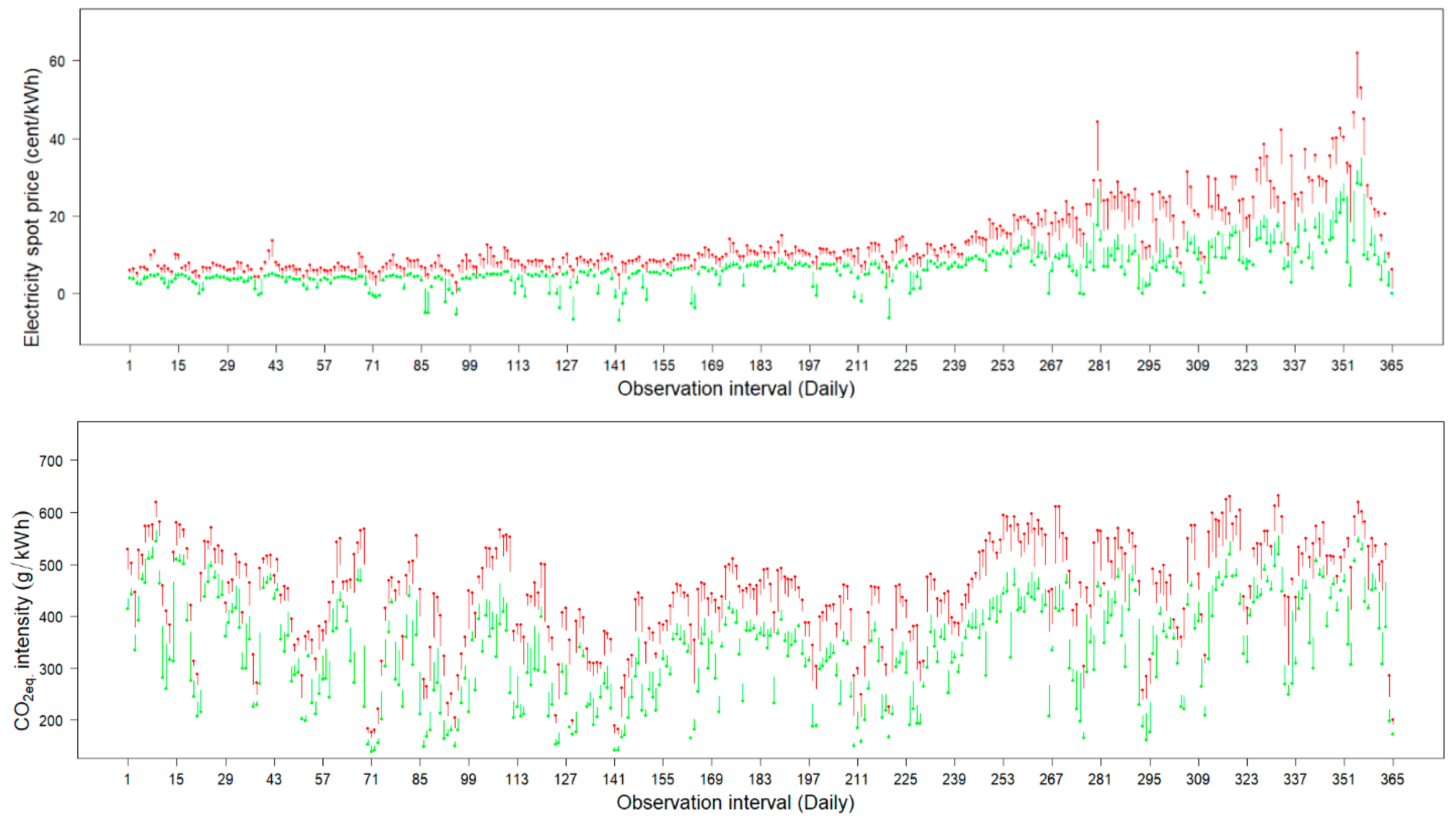
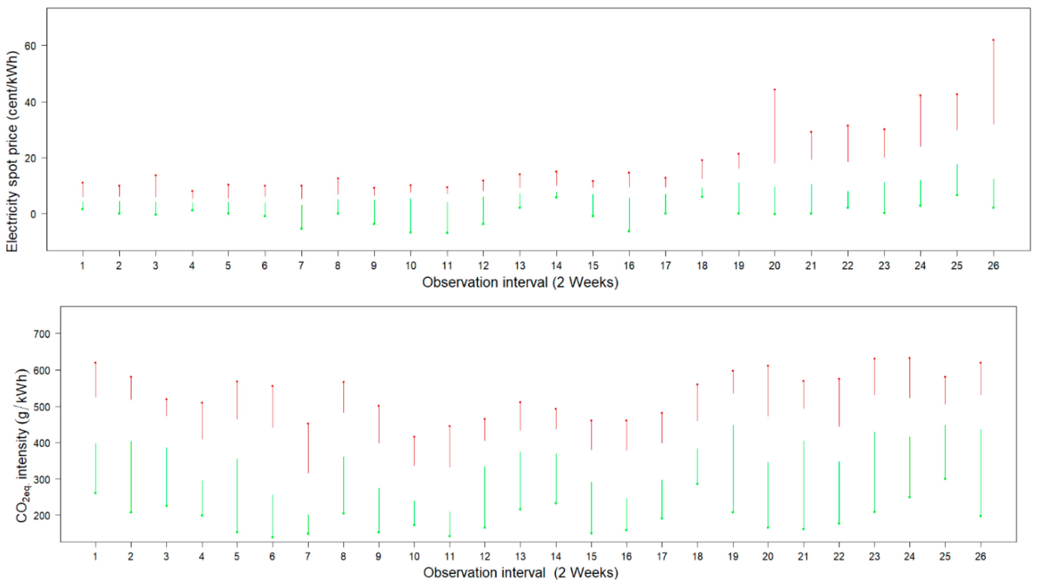
2.2. Threshold Calculation

Thresholds, which represent the boundary points for applying energy flexibility, were dynamically determined based on the observation time and the penalty signal, which in this study are CO_2eq. intensity and electricity spot price. In some studies, the observation time is chosen to be “daily” [36,37] or “biweekly” [38]. These observation periods are time intervals at which the penalty signals are monitored and used to determine the energy flexibility thresholds. This implies that 8760 data points per year are taken and aggregated into daily and biweekly intervals.

In the meantime, to approximate the optimal solution, different studies have discussed penalty signal thresholds, which represent the level at when energy flexibility is requested from a building energy system based on this aggregated data. Ref. [39] introduced two adjustable parameters to define the top and bottom threshold for grid interaction signals. In [40], various upper and lower thresholds were used to calculate the number of hours for the set-point adjustment. The thresholds were determined with 25th and 75th percentiles in [36].

In this study, the thresholds as responding to penalty signals were defined by the upper 25% quartile (downward flexibility) and the lower 25% quartile (upward flexibility) using hourly values. Whisker plots were used to assign the penalty signals into quartile groups by percentile analysis. Subsequently, this research compared the results of both aggregation intervals based on the grid status for heating season.

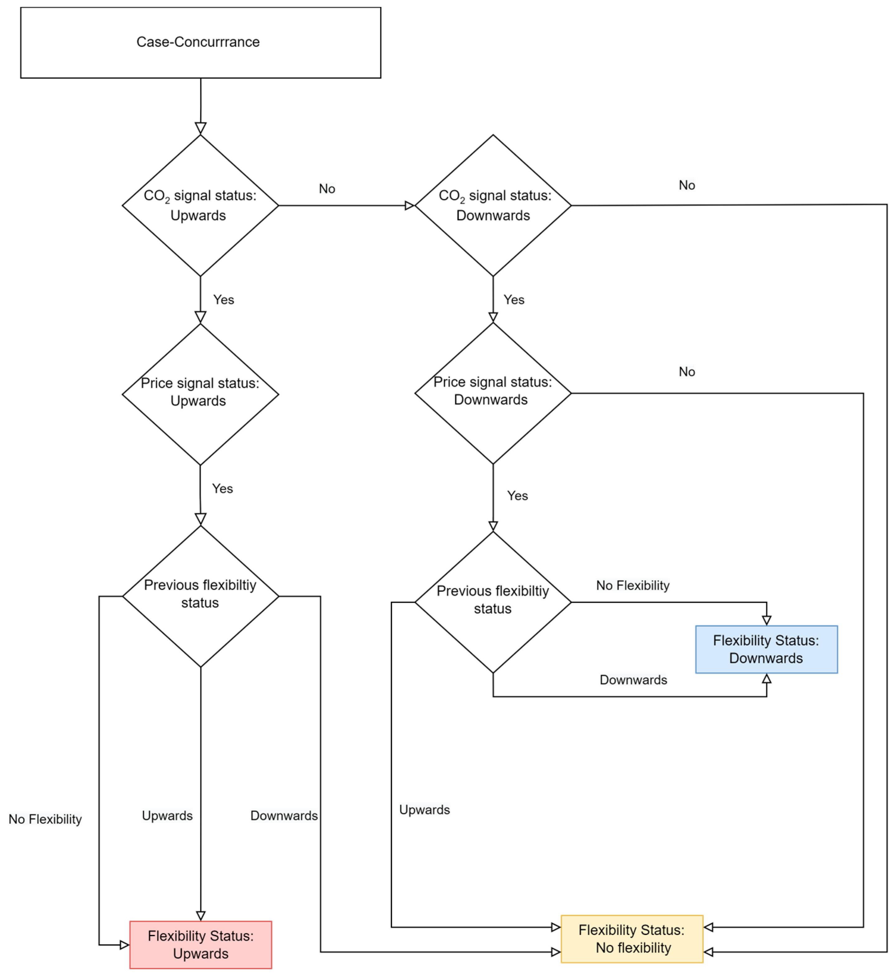
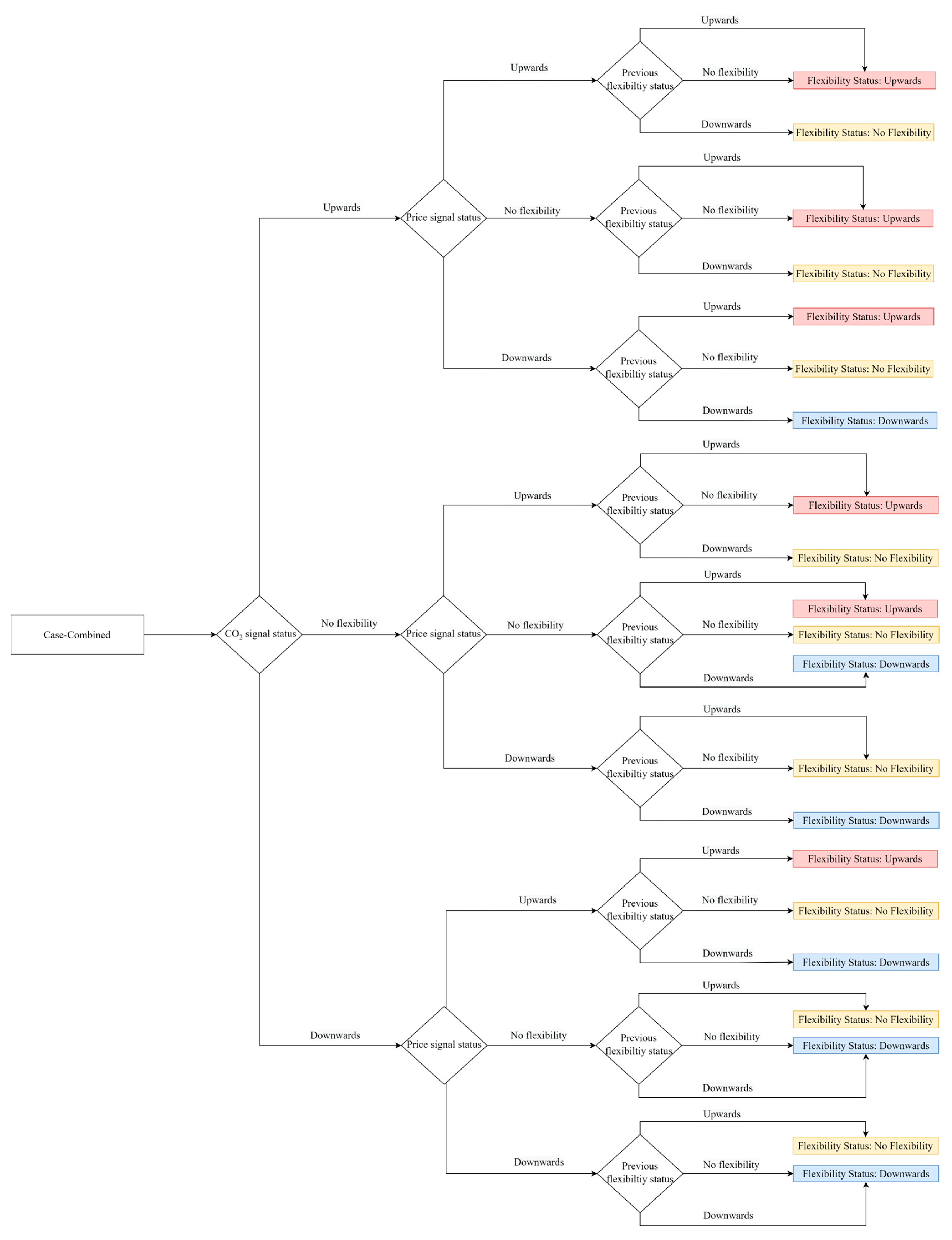
2.3. Development of Penalty Signals and the Simulation Cases

For every aggregation interval, five cases were simulated by a building energy simulation tool to quantify the total CO₂ emissions of the building energy supply, cost, and load profile according to the specified penalty signals. (

Table 3. The simulation cases based on the penalty signals.

Cases	Penalty Signal
Emission	CO2eq. intensity
Price	Electricity spot price
Concurrence	Simultaneous
Combined	Combined
Reference	Penalty unaware case—Thermostatic valve control

).

In the first case (Case Emission), the CO_2eq. intensity was exploited as a penalty signal. In the second case (Case Price), price signal was applied. In the third case (Case Concurrence), if the CO_2eq. intensity and price signal reflected the same behaviour at the same moment, such as either upward or downward interaction, this synchronised status was used as a signal (Figure 1).

In the fourth case (Case Combined), the combination of CO_2eq. intensity and price signals were driven for power grid interaction, such that if one of these signals offered interaction, it was taken into account to develop the combined status. The strategy to form this status was as follows: (1) If both signals offered the same type of power grid interaction state (upwards (+1), downwards (−1), or no interaction (0)), this state was set as the combined signal. (2) If these signals were not harmonised (one is upwards and other is downwards), the previous signal was checked and (2a) the same state as the previous combined signal was chosen; conversely, (2b) if the previous signal was 0 (no interaction), no interaction was continued. (3) If a shift from upwards to downwards or vice versa based on the signals was estimated, it was ignored, and the combined signal was considered as no interaction (Figure 2). Additionally, for (1), the previous signal was checked with the same purpose. This ensured a smooth transition between the statuses and avoided the sharp changes in the indoor thermal comfort and HVAC operation. Finally, the fifth case (Case Reference) presented the penalty signal-unaware status of the case building.

3. Results

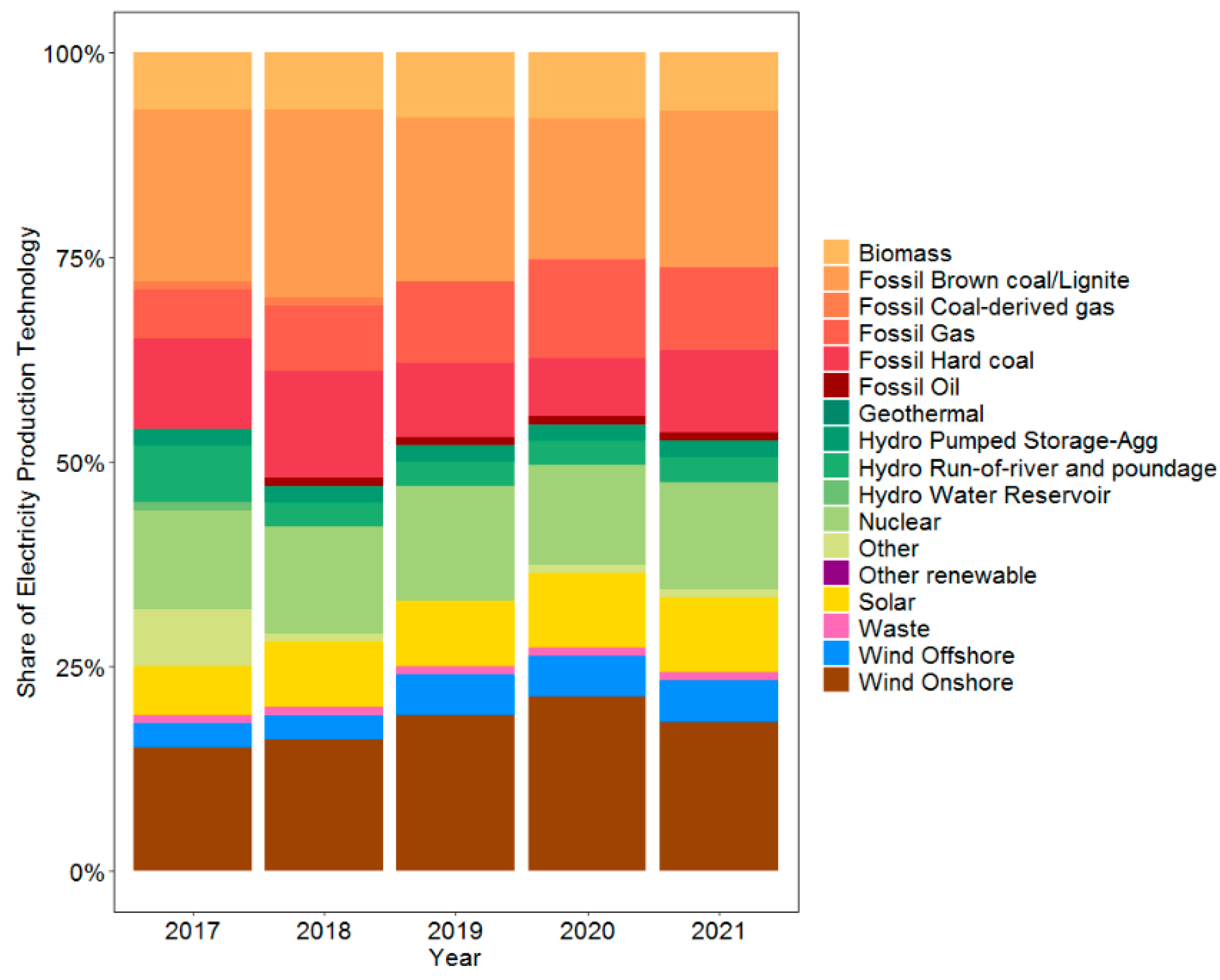
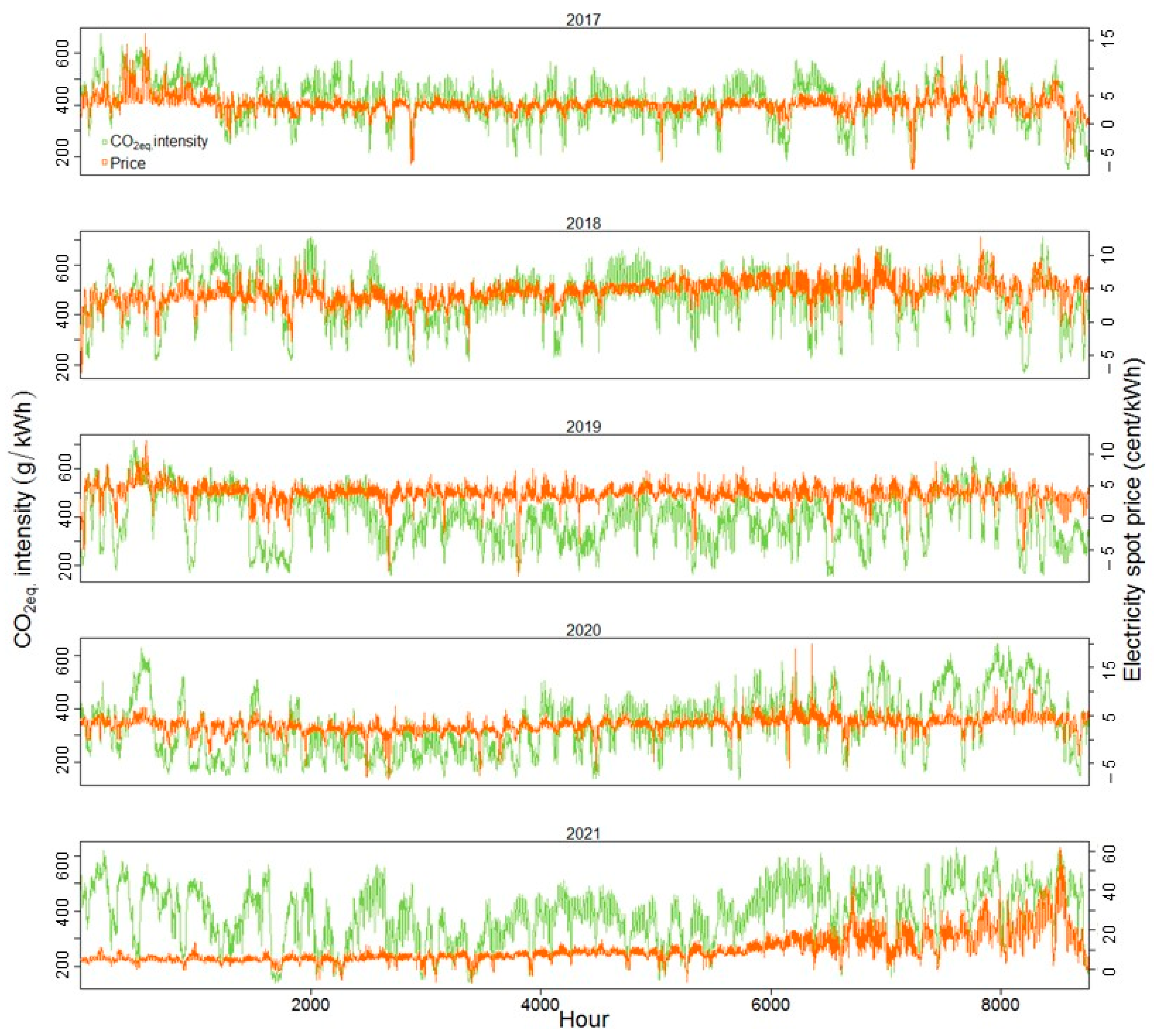
3.1. Dynamic CO_2eq. Intensity

Figure 3 presents the share of electricity production technologies between 2017 and 2021. In 2017, the largest contribution was from RES. Although the share of RES decreased in the following years, a growing trend can be observed from 2018 to 2020. Wind energy is the leading technology among RES in Germany, and its overall percentage has been increasing every year. The decreasing trend in production ratio from fossil technologies has reversed, resulting in an increase in 2021. Consequently, electricity generation from RES decreased to nearly 50% in 2021, which was attributed to unfavourable weather conditions [41]. In other words, the current generation in 2021 is approximately 50% dependent on fossil fuel-based power plants.

Figure 4 presents the grid CO_2eq. intensity and electricity spot price for the given years. The yearly average CO_2eq. intensity between 2017 and 2021 is calculated as 413, 404, 344, 311, and 439 gCO_2eq./kWh, respectively.

The share of electricity production from RES is higher in 2020 compared to other years, leading to lower CO_2eq. intensity. Conversely, the highest intensity is observed in 2021 due to a higher share of fossil-based production. The intensity value varies significantly over the year, with the average intensity being approximately 500 gCO_2eq./kWh during wintertime and around 300 gCO_2eq./kWh in the summer of 2021. The annual average values from Table 2 are reflected in Figure 4 dynamically based on hourly resolution for Germany.

The correlation between the CO_2eq. intensity and the electricity spot price is explored for the period between 2017 and 2021, and is illustrated in Figure 5. The results show an upward trend in the correlation factor over this period. As the share of RES in electricity generation increases, a stronger relationship is observed between cheaper generation and CO₂ emission-free generation, particularly between 2017 and 2020. Therefore, the behaviour of CO_2eq. intensity as a penalty signal on the energy flexibility reflects the behaviour of the price signal, especially in 2020, when the highest correlation is observed. However, a drastic change occurs in 2021, attributed to the rise of fossil-based production and the increase in electricity spot price by approximately three times compared to 2020 [41]. Further analysis of the relation between CO_2eq. intensity and the load in the power grid reveals no significant correlation, thus it is not presented in this study.

As described in Section 2.1, the CO_2eq. intensity calculation considers the CO₂ emission from the imported energy, hence, in Figure 6, the CO_2eq. intensity profile during import period is examined. One of the highest energy flows to Germany is from the Czech Republic. Along with the import, the CO_2eq. intensity in the German power grid rises.

3.2. Penalty Signals Threshold

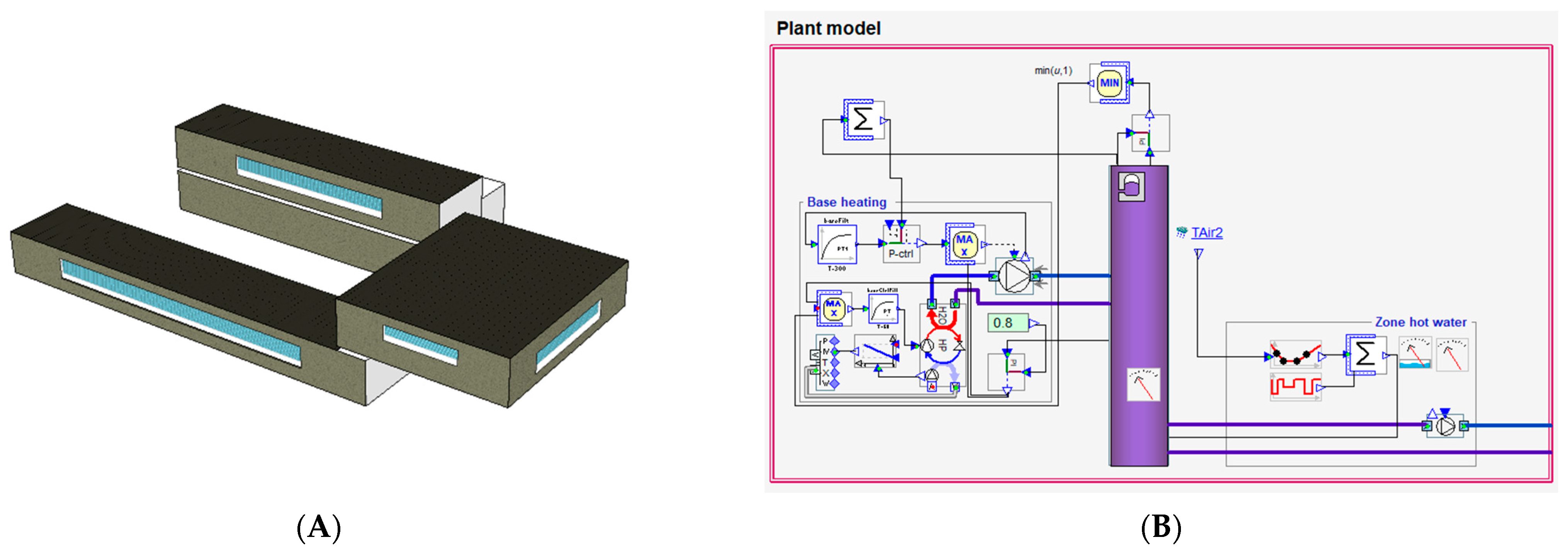
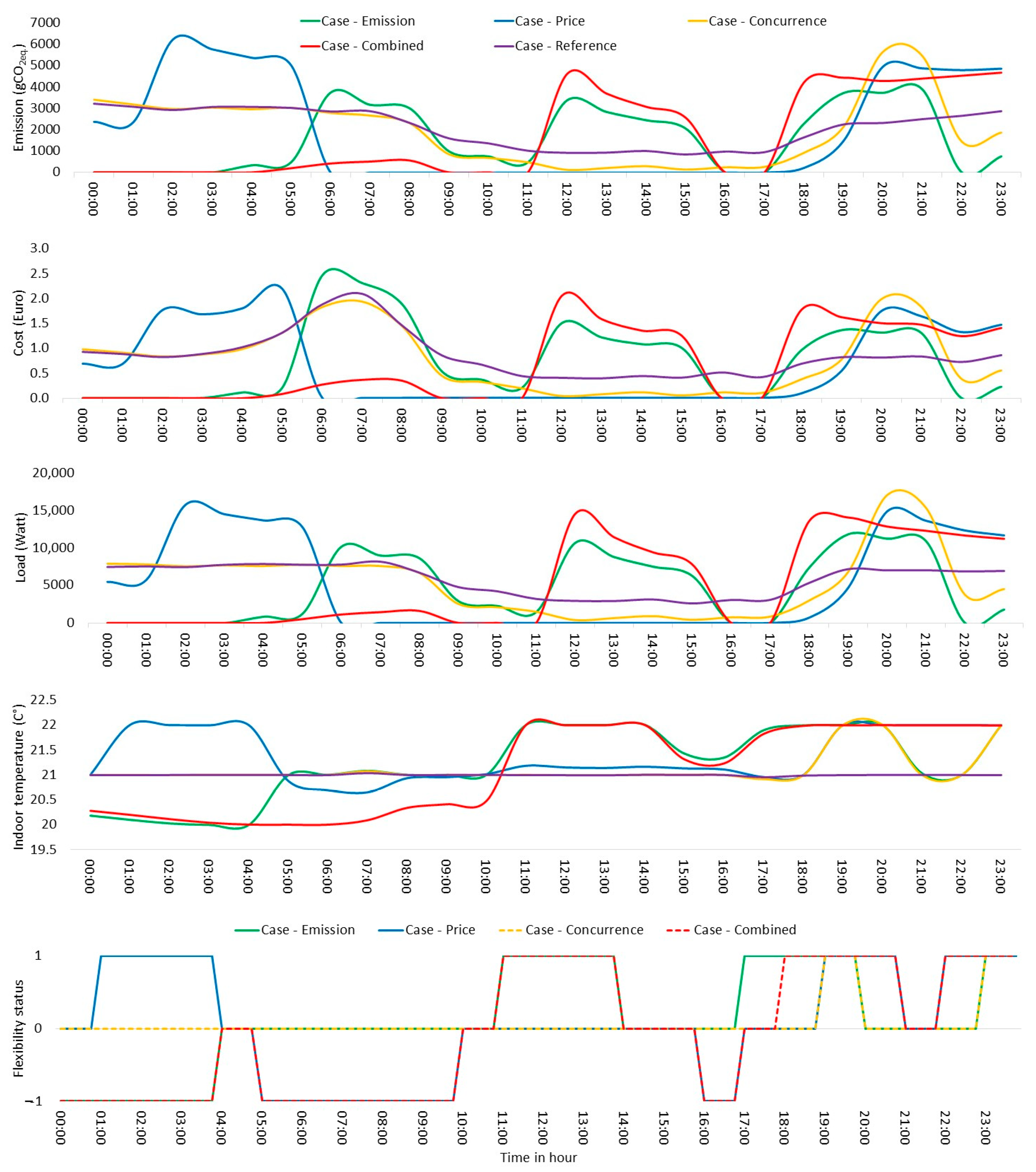
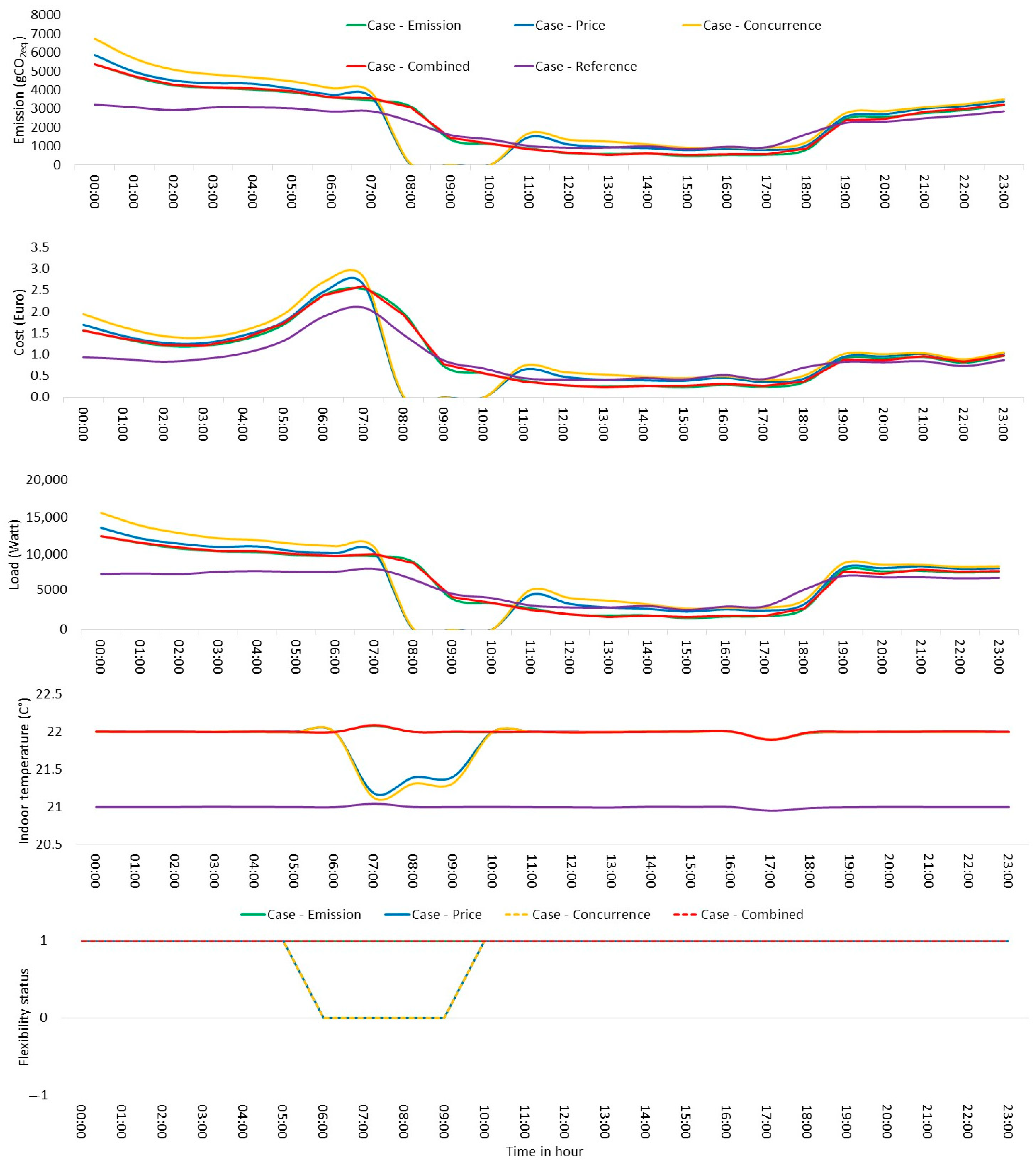
Figure 7 presents the penalty signal thresholds for CO_2eq. intensity and electricity spot price for daily aggregation in 2021. The price thresholds vary for each daily aggregation and fluctuate over the course of the year. This raises concerns about the choice of a threshold for a particular day, e.g., selecting the threshold for day_n may result in no positive grid interaction on day_n+1 or a loss of potential flexibility application hours. Similarly, CO_2eq. intensity thresholds vary significantly between days, requiring a threshold to be set for each day. Additionally, the daily CO_2eq. intensity thresholds exhibit larger differences throughout the year than the electricity spot price thresholds.

Figure 8 shows the results for biweekly aggregation, with a total of 26 intervals over the course of a year. The electricity spot price threshold values are close to each other among observations than those at daily aggregation, although differences are observed among the seasons. Conversely, CO_2eq. intensity threshold exhibits distinct variations during the year.

The benchmark for threshold limits for CO_2eq. intensity signal and price signal between daily and biweekly aggregation was assessed using the upper quartile and lower quartile for the heating season, and the results with the maximum possible flexibility operation hours are presented in

Table 4. The thresholds of CO_2eq. intensity based on daily and biweekly aggregation—heating season.

	Daily—CO2eq. Intensity Signal				Biweekly—CO2eq. Intensity Signal
	Upper	Lower	Upward	Downward	Upper	Lower	Upward	Downward
	(gCO2eq./kwh)		(Hour)		(gCO2eq./kwh)		(Hour)
Day 1	481	447	6	5	531	435	24	0
Day 2	499	465	6	6			7	2
Day 3	527	467	6	5			3	2
Day 4	494	440	6	7			0	9
Day 5	473	333	5	6			7	2
Day 6	553	513	7	5			14	2
Day 7	515	492	6	7			0	23
Day 8	539	497	6	5			0	10
Day 9	481	408	5	7			0	15
Day 10	508	456	7	5			13	2
Day 11	499	473	6	6			4	6
Day 12	464	426	6	6			0	4
Day 13	488	453	5	5			13	0
Day 14	513	481	6	6			0	2

and

Table 5. The thresholds of price signal based on daily and biweekly observation intervals in the heating season. (Data source for electricity spot price: [29]).

	Daily—Price Signal				Biweekly—Price Signal
	Upper	Lower	Upward	Downward	Upper	Lower	Upward	Downward
	(cent/kwh)		(Hour)		(cent/kwh)		(Hour)
Day 1	23	17	5	6	32	12	19	0
Day 2	21	9	6	6			6	0
Day 3	33	19	7	6			12	0
Day 4	29	13	5	6			3	11
Day 5	24	10	6	6			8	1
Day 6	34	20	7	6			9	0
Day 7	28	20	5	6			2	13
Day 8	28	21	7	6			3	2
Day 9	24	11	5	6			1	0
Day 10	32	19	7	6			12	0
Day 11	37	20	6	6			5	13
Day 12	34	24	6	6			4	14
Day 13	41	26	6	6			0	14
Day 14	39	27	5	6			0	16

. The penalty-aware times are grouped into upward and downward periods. Upward time represents the hours during a day when the penalty signal is less than the lower limit and downward time stands for the periods when the dynamic signal is higher than the upper limit. In Table 4, the differences between aggregations are found as following: In daily aggregation, flexibility application is possible while dynamic CO_2eq. intensity signal is higher than 481 gCO_2eq./kwh or lower than 447 gCO_2eq./kwh for Day 1. The maximum possible flexibility operation hours from the grid side are 6 and 5 h for upward and downward action, respectively. In the case of biweekly aggregation, there can be flexibility when the CO_2eq. intensity signal is higher than 531 gCO_2eq./kwh and lower than 435 gCO_2eq./kwh on the same day, and these are the limits for the next 13 days. On Day 1, the entire day is offered for the upward energy flexibility. By the last day, Day 14, almost no interaction presents based on the calculation results of biweekly aggregation. For this day, 6 h of upward and downward actions are found by the daily aggregation. Comparing the daily and biweekly aggregation cases, a 50% difference is observed for threshold limits, which is the main factor for the variability seen for possible flexibility hours. Besides, rather than having a switch between upward and downward actions, as in the daily aggregation case, the building is intended to have one type of operation in biweekly aggregation.

Table 5 presents the thresholds for the price signal and the maximum possible interaction hours for the heating season. Similar to the CO_2eq. intensity signal case, the daily aggregation case shows 5 and 6 h of upward and downward action on Day 1, respectively. However, some days exhibit significant differences by biweekly aggregation by enabling 19 h of upwards flexibility. On Day 14, the flexibility by biweekly aggregation is found as 16 h of downward flexibility. Yet, nearly equal number of flexibility hours (5 and 6 h) for both upwards and downwards are possible with daily aggregation.

4. A Case Study

The threshold limits are applied to the office zones of a university building assumed to be equipped with an air source heat pump with a constant COP of 4. The university building is located in Wuppertal, Germany and has a total net floor area of 860 m² (only for the case zone as presented in Figure 9).

The simulation employs measured climate data from the university weather station and power grid CO_2eq. intensity and electricity spot price data from 2021 as penalty signals. The U-values of the external walls (0.22 W/m².K), window (1.3 W/m².K), roof (0.20 W/m².K) and floor (0.28 W/m².K) were defined as well as the occupancy and ventilation profile (Mon.–Fri. 8:00 a.m. to 6:00 p.m.) in the simulation model. The indoor air temperature set points are designated as the flexibility option.

The simulation was conducted in hourly time step resolution using the IDA-ICE simulation tool [42], and all five cases are simulated, as outlined in Section 2.3. Daily and biweekly aggregation intervals are used for the simulation for a year, and a rule-based control (RBC) algorithm is employed. The calculated thresholds from Section 3.2 are inserted as input into the control macro, and the indoor temperature levels are adjusted according to the input flexibility status. The indoor temperature set points are 20 °C, 21 °C, and 22 °C for downward flexibility status, no flexibility status and upward flexibility status, respectively, during the heating season. Figure 10 presents the emissions, cost based on the electricity spot market prices (not end user costs), load demand profile, indoor temperature, and the possible flexibility status for Day 1 (from Table 4) as a representative day during the heating season based on daily aggregation, while Figure 11 presents the same metrics for biweekly aggregation intervals (Day 1 from Table 5). The analysis and comparison of the results of the entire 14 days are given in

Table 6. The results of the simulated cases for two weeks—heating season.

	Case Emission		Case Price		Case Concurrence		Case Combined		Case Reference
	1 Day	2 W	1 Day	2 W	1 Day	2 W	1 Day	2 W	-
Load demand (kWh)	690	710	715	740	740	730	710	740	875
CO2 emission (kgCO2eq.)	620	615	690	650	685	690	665	640	840
Cost (Euro)	310	280	245	240	300	305	290	250	380

with the reference case results. In this research, a simple thermostatic case is simulated for the reference case, and the given costs represent electricity usage coming from the heat pump operation, excluding other zone usage-related costs. It is assumed that end user costs follow the spot market cost profile.

The minimisation objective is achieved for both daily and biweekly aggregation as illustrated in Figure 10 and Figure 11. The results comparison of observation intervals indicates that savings are higher on biweekly aggregation intervals except for Case Concurrence. In Case Emission, CO₂ emissions are reduced by 26% and 27% with daily and biweekly aggregation, respectively. In Case Price, around a 35% decrement of costs is observed. In Case Concurrence, emission is reduced by 18%, while the cost change is reduced by around 27%. In Case Combined, a 21% and 24% downward change on emissions, besides, a 24% and 34% less cost is calculated for daily and biweekly aggregation, respectively.

Table 7. The results of the simulated cases for entire heating season in a year.

	Case Emission		Case Price		Case Concurrence		Case Combined		Case Reference
	1 Day	2 W	1 Day	2 W	1 Day	2 W	1 Day	2 W	-
Load demand (kWh)	20,800	22,200	20,400	21,350	21,000	22,000	20,800	21,700	23,300
CO2 emission (kgCO2eq.)	5660	5900	6170	6120	6240	6260	5900	5960	8290
Cost (Euro)	1500	1450	1270	1300	1530	1515	1360	1330	2070

provides a comprehensive overview of the yearly savings achieved by the different cases during the heating season. Based on the optimisation parameter (such as emissions for Case Emission and cost for Case Price, etc.), higher savings are calculated in the daily aggregation interval case by a small margin. Case Price results in the highest cost savings, followed by Case Combined. Likewise, the difference in emission savings between Case Emission and Case Combined is negligible. Although the results of Case Concurrence exhibit improvement compared to the reference case, they do not yield any substantial advantage in terms of final metrics. Single penalty signals, such as CO_2eq. intensity and price signals, maximise savings for their respective optimisation parameters. However, a holistic optimisation approach can be achieved as demonstrated by Case Combined.

5. Discussion

The relation between CO_2eq. intensity and share of electricity production type are assessed between 2017 and 2021. Following this, the correlation of CO_2eq. intensity and electricity spot price is analysed. The decrement of the positive correlation in the last year is highlighted. Moreover, it is seen that the CO_2eq. intensity does not depend on local generation technologies but also on the CO_2eq. intensity of the interconnected countries. The expansion of the power grid through neighbouring countries limits the value of environmental returns of the existing local RES. Despite the ongoing action plan and the increasing penetration of RES, the share of fossil-fuel based electricity generation does not demonstrate a steady decrease. For a nonemission power grid, the operated generation technology types of the interconnected countries are critical as the local technologies.

Two joint penalty signals and their modelling approach with the motivation of acquiring both environmental and economic savings are introduced. In addition to a single type of penalty signal implementation, their joint impact was able to address improved performance in terms of environment, cost, and load demand. The results from Case Combined presents an option for building operations which ensure remarkable savings on metrics compared to the other cases. Even though each of these parameters can be enhanced more by individual signals (either CO_2eq. or price), the overall average outcome is found to be favourable.

The building energy flexibility analysis by applying different penalty signals considering the upper and lower quartiles was performed with the calculated power grid CO_2eq. intensity data and historical electricity spot price (before tax) data from the ENTSO-E platform. Two aggregation intervals, namely daily and biweekly, were used for threshold analysis. These thresholds were incorporated into two joint penalty signals as concurrence and combined signals. The approach to develop these signals was described. An office zone group’s energy performance, presenting CO₂ emission, cost, load demand, and indoor temperature, was simulated by a building energy simulation tool using the mentioned penalty signals for five given cases. The main findings are listed below:

• The approach for aggregation intervals of penalty signals plays a critical role for the determination of thresholds and the maximum possible interaction hours from the grid side. In the heating season, marked differences were observed for upper and lower thresholds between aggregation intervals.
• Biweekly aggregation intervals might provide an improved building performance based on the time of the year during heating season. However, no significant difference is found between aggregation intervals in the yearly metrics.
• With Case Combined, the environmental and economic performance closely approximates that of Case Emission and Case Price, respectively, thereby achieving the research’s objective of minimizing both metrics to nearly the same level.
• Biweekly aggregation reduces peak demand compared to daily aggregation and results in less indoor temperature fluctuation.

The modelling approach of the combined signal ensures more flexibility hours than a single penalty signal, thereby improving both environmental and economic metrics with the use of a joint signal.

6. Conclusions

A simple-structured methodology is presented to calculate the dynamic climate gas emission intensity in the power grid. The calculation method can be used to generate the CO₂ penalty signal in the energy flexibility studies. The main drivers of the emission signals were investigated, following the impact of production technology types, and their share and electricity import in the local power grid are discussed. The relation of CO_2eq. intensity was compared to electricity spot price and energy use as a penalty signal in energy flexibility. The biggest challenge was to collect reliable climate gas emission factors of the production technologies and the average emission intensity of the countries, because available data from various sources are not consistent. However, data of electricity production from technologies was easily accessible through transparency platform. For precise emission intensity calculation, the dynamic CO_2eq. intensity of the interconnected countries should be considered rather than the average value for energy trade. However, this would complicate the calculation process, especially if there is more than one bidding zone in the connected country. As the penetration of RES is increasing in Germany, a bidding zone configuration might be needed to ensure congestion management. In such a situation, the grid emission intensity in Germany should be calculated on a bidding zone basis and the relation with the price signal should be assessed separately. Additionally, the self-consumption of the production plants should be considered for a more accurate outcome.

A joint signal is necessary for the current mixed power grid but may not be required for future grids based solely on renewable energy sources. In such a scenario, the order of merit for electricity generation could change, potentially simplifying the calculation challenges of marginal emission factors. Then, the dynamic power grid intensity and electricity spot prices would be positively correlated and employed in building energy flexibility applications.

References

1. Climate Action, 2030 Climate Target Plan. Available online: https://ec.europa.eu/clima/eu-action/european-green-deal/2030-climate-target-plan_en (accessed on 5 August 2022).
2. Communication from The Commission to The European Parliament, The Council, The European Economic and Social Committee and The Committee of the Regions. 2020. Available online: https://eur-lex.europa.eu/legal-content/EN/TXT/?uri=CELEX:52020DC0562 (accessed on 5 August 2022).
3. Federal Ministry for the Environment, Nature Conservation, Building and Nuclear Safety (BMUB). Climate Action Plan 2050: Principles and Goals of the German Government’s Climate Policy. 2016. Available online: https://www.bmuv.de/en/publication/climate-action-plan-2050-en (accessed on 3 March 2023).
4. Climate Change Act: Climate Neutrality by 2045. Available online: https://www.bundesregierung.de/breg-de/themen/klimaschutz/climate-change-act-2021-1936846 (accessed on 7 August 2022).
5. Lashmar, N.; Wade, B.; Molyneaux, L.; Ashworth, P. Motivations, barriers, and enablers for demand response programs: A commercial and industrial consumer perspective. Energy Res. Soc. Sci. 2022, 90, 102667. [Google Scholar] [CrossRef]
6. Bando, S.; Sasaki, Y.; Asano, H.; Tagami, S. Balancing control method of a microgrid with intermittent renewable energy generators and small battery storage. In Proceedings of the 2008 IEEE Power and Energy Society General Meeting—Conversion and Delivery of Electrical Energy in the 21st Century, Pittsburgh, PA, USA, 20–24 July 2008; pp. 1–6. [Google Scholar]
7. Makolo, P.; Zamora, R.; Lie, T.-T. The role of inertia for grid flexibility under high penetration of variable renewables—A review of challenges and solutions. Renew. Sustain. Energy Rev. 2021, 147, 111223. [Google Scholar] [CrossRef]
8. Eto, J.H.; Alvarado, F.L.; Dagle, J.E.; Hauer, J.F.; Widergren, S.E.; Gross, G.; Overbye, T.; Hirst, E.; Kirby, B.; Meyer, D.; et al. National Transmission Grid Study. 2002. Available online: http://energy.gov/oe/downloads/national-transmission-grid-study-2002 (accessed on 3 March 2023).
9. Executive Office of the President. Economic Benefits of Increasing Electric Grid Resilience to Weather Outages; Technical Report; President’s Council of Economic Advisers and the U.S. Department of Energy’s Office of Electricity Delivery and Energy Reliability: Washington, DC, USA, 2013.
10. Sahari, A. Electricity prices and consumers’ long-term technology choices: Evidence from heating investments. Eur. Econ. Rev. 2019, 114, 19–53. [Google Scholar] [CrossRef]
11. Li, J.; Ge, S.; Liu, H.; Zhang, S.; Wang, C.; Wang, P. Distribution locational pricing mechanisms for flexible interconnected distribution system with variable renewable energy generation. Appl. Energy 2023, 335, 120476. [Google Scholar] [CrossRef]
12. Kroposki, B.; Johnson, B.; Zhang, Y.; Gevorgian, V.; Denholm, P.; Hodge, B.M.; Hannegan, B. Achieving a 100% Renewable Grid: Operating Electric Power Systems with Extremely High Levels of Variable Renewable Energy. IEEE Power Energy Mag. 2017, 15, 61–73. [Google Scholar] [CrossRef]
13. Knaut, A. Essays on the Integration of Renewables in Electricity Markets; Köln Universität: Köln, Germany, 2017; Available online: https://kups.ub.uni-koeln.de/7729/ (accessed on 25 February 2023).
14. Widuto, A. Reforming the EU Electricity Market; European Parliamentary Research Service: Brussels, Belgium, 2023. [Google Scholar]
15. European Union Agency for the Cooperation of Energy Regulators. Energy Bills Continue to Be Very Different across EU Member States: The new Energy Retail and Consumer Protection Volume. Available online: https://documents.acer.europa.eu/Media/News/Pages/Energy-bills-continue-to-be-very-different-across-EU-Member-States.aspx (accessed on 3 March 2023).
16. Dahl Knudsen, M.; Petersen, S. Demand response potential of model predictive control of space heating based on price and carbon dioxide intensity signals. Energy Build. 2016, 125, 196–204. [Google Scholar] [CrossRef]
17. Saberi, K.; Pashaei-Didani, H.; Nourollahi, R.; Zare, K.; Nojavan, S. Optimal performance of CCHP based microgrid considering environmental issue in the presence of real time demand response. Sustain. Cities Soc. 2019, 45, 596–606. [Google Scholar] [CrossRef]
18. Hawkes, A.D. Estimating marginal CO2 emissions rates for national electricity systems. Energy Policy 2010, 38, 5977–5987. [Google Scholar] [CrossRef]
19. Bigazzi, A. Comparison of marginal and average emission factors for passenger transportation modes. Appl. Energy 2019, 242, 1460–1466. [Google Scholar] [CrossRef]
20. Fleschutz, M.; Bohlayer, M.; Braun, M.; Henze, G.; Murphy, M.D. The effect of price-based demand response on carbon emissions in European electricity markets: The importance of adequate carbon prices. Appl. Energy 2021, 295, 117040. [Google Scholar] [CrossRef]
21. Zohrabian, A.; Mayes, S.; Sanders, K.T. A data-driven framework for quantifying consumption-based monthly and hourly marginal emissions factors. J. Clean. Prod. 2023, 396, 136296. [Google Scholar] [CrossRef]
22. Bardwell, L.; Blackhall, L.; Shaw, M. Emissions and prices are anticorrelated in Australia’s electricity grid, undermining the potential of energy storage to support decarbonisation. Energy Policy 2023, 173, 113409. [Google Scholar] [CrossRef]
23. Song, M.; Alvehag, K.; Widén, J.; Parisio, A. Estimating the impacts of demand response by simulating household behaviours under price and CO2 signals. Electr. Power Syst. Res. 2014, 111, 103–114. [Google Scholar] [CrossRef]
24. Wu, J. Scheduling Smart Home Appliances in the Stockholm Royal Seaport; School of Electrical Engineering, Automatic Control, KTH Royal Institute of Technology: Stockholm, Sweden, 2012. [Google Scholar]
25. Setlhaolo, D.; Xia, X. Combined residential demand side management strategies with coordination and economic analysis. Int. J. Electr. Power Energy Syst. 2016, 79, 150–160. [Google Scholar] [CrossRef]
26. Pooranian, Z.; Abawajy, J.H.; Conti, M. Scheduling Distributed Energy Resource Operation and Daily Power Consumption for a Smart Building to Optimize Economic and Environmental Parameters. Energies 2018, 11, 1348. [Google Scholar] [CrossRef]
27. Zhang, D.; Evangelisti, S.; Lettieri, P.; Papageorgiou, L.G. Economic and environmental scheduling of smart homes with microgrid: DER operation and electrical tasks. Energy Convers. Manag. 2016, 110, 113–124. [Google Scholar] [CrossRef]
28. Nilsson, A.; Stoll, P.; Brandt, N. Assessing the impact of real-time price visualization on residential electricity consumption, costs, and carbon emissions. Resour. Conserv. Recycl. 2017, 124, 152–161. [Google Scholar] [CrossRef]
29. ENTSO-E Transparency Platform. Available online: https://transparency.entsoe.eu/dashboard/show (accessed on 8 July 2022).
30. Bavarian State for the Environment. Calculate Your Greenhouse Gas Emissions with the CO2 Calculator. Available online: https://www.umweltpakt.bayern.de/energie_klima/fachwissen/217/berechnen-sie-ihre-treibhausgasemissionen-mit-co2-rechner (accessed on 16 August 2022).
31. European Environment Agency. CO2 Emission Intensity from Electricity Generation. Available online: https://www.eea.europa.eu/data-and-maps/daviz/sds/co2-emission-intensity-from-electricity-generation-5/@@view (accessed on 16 August 2022).
32. Carbon Footprint. Country Specific Electricity Grid Greenhouse Gas Emissions Factors. Available online: https://www.carbonfootprint.com/docs/2019_06_emissions_factors_sources_for_2019_electricity.pdf (accessed on 16 August 2022).
33. Nowtricity. CO2 Emissions Per kWh in Norway. Available online: https://www.nowtricity.com/country/norway/ (accessed on 16 August 2022).
34. European Environment Agency. Greenhouse Gas Emission Intensity of Electricity Generation by Country. Available online: https://www.eea.europa.eu/data-and-maps/daviz/co2-emission-intensity-9/#tab-chart_2_filters=%7B%22rowFilters%22%3A%7B%22ugeo%22%3A%5B%22Germany%22%5D%7D%3B%22columnFilters%22%3A%7B%7D%7D (accessed on 16 August 2022).
35. Statista. Emissions. Available online: https://www.statista.com/markets/408/topic/949/emissions/#overview (accessed on 16 August 2022).
36. Hall, M.; Geissler, A. Comparison of Flexibility Factors and Introduction of A Flexibility Classification Using Advanced Heat Pump Control. Energies 2021, 14, 8391. [Google Scholar] [CrossRef]
37. Clauß, J.; Stinner, S.; Solli, C.; Lindberg, K.B.; Madsen, H.; Georges, L. Evaluation Method for the Hourly Average CO2eq. Intensity of the Electricity Mix and Its Application to the Demand Response of Residential Heating. Energies 2019, 12, 1345. [Google Scholar] [CrossRef]
38. Le Dréau, J.; Heiselberg, P. Energy flexibility of residential buildings using short term heat storage in the thermal mass. Energy 2016, 111, 991–1002. [Google Scholar] [CrossRef]
39. Georges, E.; Garsoux, P.; Masy, G.; d’Aertrycke, G.D.; Lemort, V. (Eds.) Analysis of the flexibility of Belgian residential buildings equipped with heat pumps and thermal energy storage. In Proceedings of the CLIMA 2016 Conference and 12th REHVA World Congress, Aalborg, Denmark, 22–25 May 2016. [Google Scholar]
40. Clauß, J.; Stinner, S.; Sartori, I.; Georges, L. Predictive rule-based control to activate the energy flexibility of Norwegian residential buildings: Case of an air-source heat pump and direct electric heating. Appl. Energy 2019, 237, 500–518. [Google Scholar] [CrossRef]
41. Fraunhofer Institute for Solar Energy Systems ISE. Public Net Electricity Generation in Germany in 2021: Renewables Weaker Due to Weather—Fraunhofer ISE. Available online: https://www.ise.fraunhofer.de/en/press-media/news/2022/public-net-electricity-in-germany-in-2021-renewables-weaker-due-to-weather.html (accessed on 10 August 2022).
42. Equa Simulation AB, IDA Indoor Climate and Energy 4.8. 2018. Available online: https://www.equa.se/en/ (accessed on 20 September 2022).
Figure 1. Development of concurrence signal based on the CO2eq. intensity and price signal.
Buildings 13 01338 g001
Figure 2. Development of combined signal based on the CO2eq. intensity and price signal.
Buildings 13 01338 g002
Figure 3. The share of electricity generation technologies in Germany between 2017 and 2021 (Data source: [29]).
Buildings 13 01338 g003
Figure 4. Hourly CO2eq. intensity and electricity spot price between 2017 and 2021 (Data source for electricity spot price: [29]).
Buildings 13 01338 g004
Figure 5. Correlation of hourly CO2eq. intensity and electricity spot price (Data source for electricity spot price: [29]).
Buildings 13 01338 g005
Figure 6. Correlation of hourly CO2eq. intensity and imports with interconnected countries.
Buildings 13 01338 g006
Figure 7. Upper and lower threshold of price and CO2eq. signals with daily observation (red lines represent the upper 25th percentile (downward action) and green lines show the lower 25th percentile (upward action)).
Buildings 13 01338 g007
Figure 8. Upper and lower threshold of price and CO2eq. signals with 2 weeks’ observation (red lines represent the upper 25th percentile (downward action) and green lines show the lower 25th percentile (upward action)).
Buildings 13 01338 g008
Figure 9. (A) The building zone and (B) plant model for the simulated case.
Buildings 13 01338 g009
Figure 10. Simulation results of penalty signal with daily aggregation threshold—heating season.
Buildings 13 01338 g010
Figure 11. Simulation results of penalty signal with a biweekly observation threshold—heating season.
Buildings 13 01338 g011