1. Introduction
Infrared thermography is an advanced technique of obtaining the intensity of heat radiation invisible to the human eye. The measurements are performed with no contact between the object that is emitting heat and the measuring device (thermal camera). The result of the measurements is an image of temperature distribution on the tested surface, commonly referred to as a thermogram. Surfaces with the same temperature are usually presented using the same color.
As far as the application of this method in the building sector is concerned, its greatest impact lies in the assessment of thermal losses through different elements of the building envelope. It is usually applied in the context of improving the energy efficiency of buildings (for example: detection and identification of thermal bridges, detection of thermal irregularities, determination of building envelope thermal properties) [
1,
2]. Another application of this method is in the detection of damage (cracks) in reinforced concrete elements, such as bridges [
3]. It is also used as a measure of inhomogeneity in certain building materials, as well as for inspection of heating and electrical installations [
4].
This paper is focused on a less well known application of infrared thermography, temperature measurement during an early age hydration of cement paste, a known exothermic process. Due to this reaction, the maximum temperature of concrete can reach up to 60 °C to 70 °C in the core, while the high temperature differential between the concrete’s surface and core can result in tensile stresses followed by cracking [
5,
6].
One of the methods used for reducing the temperature development in the early phases of the hydration process is the addition of supplementary cementitious materials (SCMs) as a partial replacement of pure Portland cement (PC). The most common mineral admixtures used for this purpose are fly ash (FA), steel slag (SS), ground granulated blast-furnace slag (GGBS), and natural pozzolanic materials [
7,
8]. Zhang et al. [
9] investigated the effects of different SCMs on hydration heat and temperature of cement pastes. Four types of pastes were tested, one ordinary Portland cement paste and three pastes where 40% of Portland cement was replaced with FA, SS, and GGBS. As expected, the highest temperature was reached for the sample containing only pure cement paste (54 °C), while the temperatures for three other pastes were lower, reaching 39.8 °C for the paste containing GGBS, 38.4 °C for the paste containing SS, and 37 °C for the paste containing FA. The authors also concluded that addition of these SCMs did not change the type of hydration products of the paste system at the early ages.
Liu et al. [
10] developed a hydration temperature test device to evaluate the effects of various steel slags with potential hydraulic activity on different properties of cement pastes. The hydration temperature results showed that when the slag content was higher than 30%, the maximum hydration temperature of the cement paste decreased linearly with increasing slag content.
Almattarneh et al. [
11] followed the development of the hydration process of two cement pastes—one with pure Portland cement and the other where 20% of the cement was replaced with FA—by measuring dielectric properties during the first 24 h. Through this method, four different stages of the hydration process were detected in both pastes: stage I lasted for approximately 3 h, stage II for 7 h, stage III for 8.3 h, and finally stage IV until the end of measurements. Bentz et al. [
12] showed that the heat release curves for the first 24 h of hydration, measured using isothermal calorimetry, are very similar for cement pastes with water-to-cement ratios ranging from 0.325 to 0.425. The maximum heat flow was reached approximately 7 h after the production of samples. However, a change in the water/cement (w/c) ratio had a more distinctive influence on the semi-adiabatic temperature curves of the pastes. The peak temperature was increased when the w/c ratio was lowered from 0.425 to 0.400 to 0.350, but it did not increase when it was further lowered to 0.325. Greater differences between the heat releases of different pastes were noticed during the first 7 days of the hydration process.
Xu and Chung [
13] measured the changes in specific heat of several cement pastes using admixture surface treatments. The w/c ratio of the tested pastes was 0.35, and Portland cement type I was used in the mixtures. The authors tested 12 different pastes with the addition of as-received silica fume and silane-treated silica fume, together with carbon fibers. The reference paste containing only cement and water had a w/c ratio of 0.45 and a measured specific heat of 0.736 J/gK. The addition of silica fume influenced the increase in the cement paste specific heat by 12% and the reduction of thermal conductivity of the paste by 40% when compared to addition of silane-treated silica fume.
Azenha et al. [
14] used infrared thermography and embedded sensors to monitor the surface and internal temperatures, respectively, of a 0.4 × 0.4 × 0.4 m
3 concrete cube since casting. Emissivity was assumed constant, with an adopted value of 0.88. The cement hydration heat release was characterized with the isothermal conduction calorimetry method. The obtained results of the temperature measurements were compared with numerically calculated values using a 3D finite element model. When the measurements using a sensor placed on the surface of the tested cube and thermography in the same point were compared, they showed a very similar trend, with the sensor measuring slightly higher temperatures during the whole experiment. The highest temperature was reached at about 8.3 h after the casting of the concrete. The authors concluded that the coherence between the data collected using two different measuring techniques allowed for strong confidence in the results obtained through thermography for hardening concrete. The authors also emphasized that infrared thermography offers greater information richness regarding the temperature distribution in concrete surfaces, which cannot be obtained using other conventional temperature sensors. The drawback of the method is that it needs “visual contact” with the object in question.
Apart from the high temperature development in massive concrete structures, temperature measurements in the early age concrete are of great interest. They are applied in maturity methods in estimating the concrete strength. These methods are based on the calibration performed in laboratory conditions, as well as in situ measurements of concrete temperature development in time [
15]. Measurements of concrete and ambient temperatures are for this purpose usually conducted through embedded thermo-sensors. The thermo-sensors used for the concrete temperature measurements often cannot be reused on another element of structure, which makes these kinds of measurements very costly. Another issue connected to the use of thermo-sensors is that they measure the temperature in one point of the sample (element) volume. Development of a method that would enable measurements of temperature in a higher number of points is an object of interest both for the scientific and engineering communities. Infrared thermography is one of the proposed solutions, due to the possibility of performing measurements in many points and in this way obtaining additional information on the homogeneity of the mass.
This paper aimed to investigate the relationship between measurements performed using infrared thermography and direct temperature measurements using embedded sensors through the testing of an early age hydration process of one cement-based paste, where fly ash was used as an SCM, replacing 20% of the cement (by mass).
2. Materials and Methods
Testing the applications of a thermal camera for the measurement of temperature development in the early stages of cement paste hydration was performed on a paste consisting of pure Portland cement CEM I 42.5 N and fly ash, using water from the city pipeline.
Standard testing of the cement paste (PCP) and the cement–fly ash paste (PCFP) with 20% mass replacement of the cement was performed first. The measurement of standard consistency and setting time, according to SRPS EN 196-3:2017 [
16], was included. These results were used as initial data for the planning of the temperature measurements, since standard consistency paste was used for the preparation of samples. Moreover, in order to define the binder properties, two types of standard cement mortar (designated as PCM and PCFM) were prepared for testing of the flexural and compressive strength, according to SRPS EN 196-1:2017 [
17], at the age of 7 and 28 days. Measurements were performed on three prismatic specimens, 4 × 4 × 16 cm in size, for each type and age of testing. The breaking force for flexural strength was measured using a range between 0 and 6 kN, with the precision of 0.1 kN, and for compressive strength using range between 0 and 200 kN, with the precision of 0.25 kN. The first mortar mix consisted of pure cement, standard sand, and water (PCM), while in the second mix, 20% of cement was replaced with fly ash (PCFM).
For measurements of cement hydration temperature at the early ages, cubic concrete molds with a 10 cm edge were used. For two samples, the mold was completely filled in, while for two samples, the mold was filled up to the height of 5 cm. Cement–fly ash paste (PCFP) of a water-to-binder ratio 0.25 was used for all of the sample preparations. Two sensors were placed in each of the four samples, one in the middle (at the cross section of the cube diagonals) and another in the center of the only free side. In order not to disturb the placing of the sensors, the samples were placed and compacted by hand. The room temperature and humidity were held constant (22 °C, 50%).
2.1. Testing of Cement
The chemical composition of the cement and fly ash used in the test is presented in
Table 1, while the specific and bulk densities of the cement, fly-ash, and sand used are presented in
Table 2. Composition of the pastes and mortars tested is presented in
Table 3.
The results of the basic properties of the cement and cement–fly ash pastes used in this experiment are presented in
Table 4. The mechanical properties of the tested mortars are presented in
Table 5. The addition of fly ash led to an increase in both flexural and compressive strength at the age of 28 days. Setting time was prolonged with the addition of fly ash, which was an important information for the temperature measurements.
2.2. Temperature Measurement Setup
The effects of the heat of hydration were recorded simultaneously on all four samples using a thermal imaging camera (FLIR E6) to monitor the temperature on the surface of the samples, as well as two thermo-sensors (IC LM35) installed in the middle and on the surface of each sample. To measure, display, and record the temperature in the center and on the surface of the four samples, we developed a custom LabVIEW application connected to an eight-channel system of thermo-sensors (see details below). The ambient temperature (thermostatic laboratory) was 22 °C. Temperature monitoring of the fresh concrete lasted for 30 h, and the sampling period was 10 min.
Figure 1 shows the experimental setup used, and
Figure 2 presents the positions of the sensors in the samples. A thermal imaging camera (with an accuracy of ±2 °C) recorded a thermogram of the upper surface of the sample. To prevent the reflection of IR radiation from the environment, PVC pipes with diameters of 200 mm were used.
On the basis of the expected temperature range and the required accuracy, an integrated LM35 circuit [
18] was used as the thermo-transducer. An additional resistor (100 k) to the negative source (−5 V) enabled the measurement of negative temperatures (
Figure 3). After filtering (capacitors 10 nF) and adjustment (resistors 10 kΩ), the signals from the thermo-sensor were fed to the input channels (AI CH0 to AI CH7) of the analog-to-digital converter (NI USB 6009) [
19]. The obtained digital signals were fed into a computer (PC) via the USB port and further processed by software. The temperature transmitters themselves were factory-calibrated in the range of −40 °C to 110 °C, so no additional adjustments were required. The accuracy of the measurement was ±0.2 °C. Due to the physical dispersion of the thermal sensors, shielded conductors were used for the transmission of analog signals over a relatively large distance (several meters) for each channel separately.
An application for measuring, displaying, and storing temperature in 8 points was developed in the software package LabVIEW 2016 [
20]. The graphic code (block diagram) of the application is shown in
Figure 4. DAQ Assistant, a standard module of the LabVIEW package for data acquisition, was used to measure analog signals from thermo-transducers. The data were then separated into eight channels, averaged (Statistics), and multiplied by 100 to transform the temperature into °C (output from LM35 is 10 mV/°C). The obtained temperatures are shown on the displays Ti (°C) and diagrams (XY Ti) and finally saved in the form of a text file whose name is specified before starting the measurement. The program was able to be stopped at any time by clicking the STOP button [
21].
For clarity, separate diagrams for each of the 8 channels were included on the front panel of the virtual instrument. Numerical displays for temperature (Ti (°C)) and time (t (min)), a file name input field, the STOP button, and an error code display field were also included.
2.3. Thermal Camera Measurement Setup
Images were obtained using a FLIR E6 thermal camera positioned at a distance of 60 cm from the sample, through a tube (as presented in
Figure 1). This was done to stabilize the environment between the camera and the surface of the samples. Images were always taken in the same order, after the stabilization of the temperature.
After the finalization of the measurements (30 h), images were processed using the FLIR Tools Plus V12 software, and the reports for each sample were extracted. The processing included defining the surface from which the temperatures should be calculated and inputting the values for emissivity, reflected temperature, and atmospheric temperature, as presented in
Figure 5.
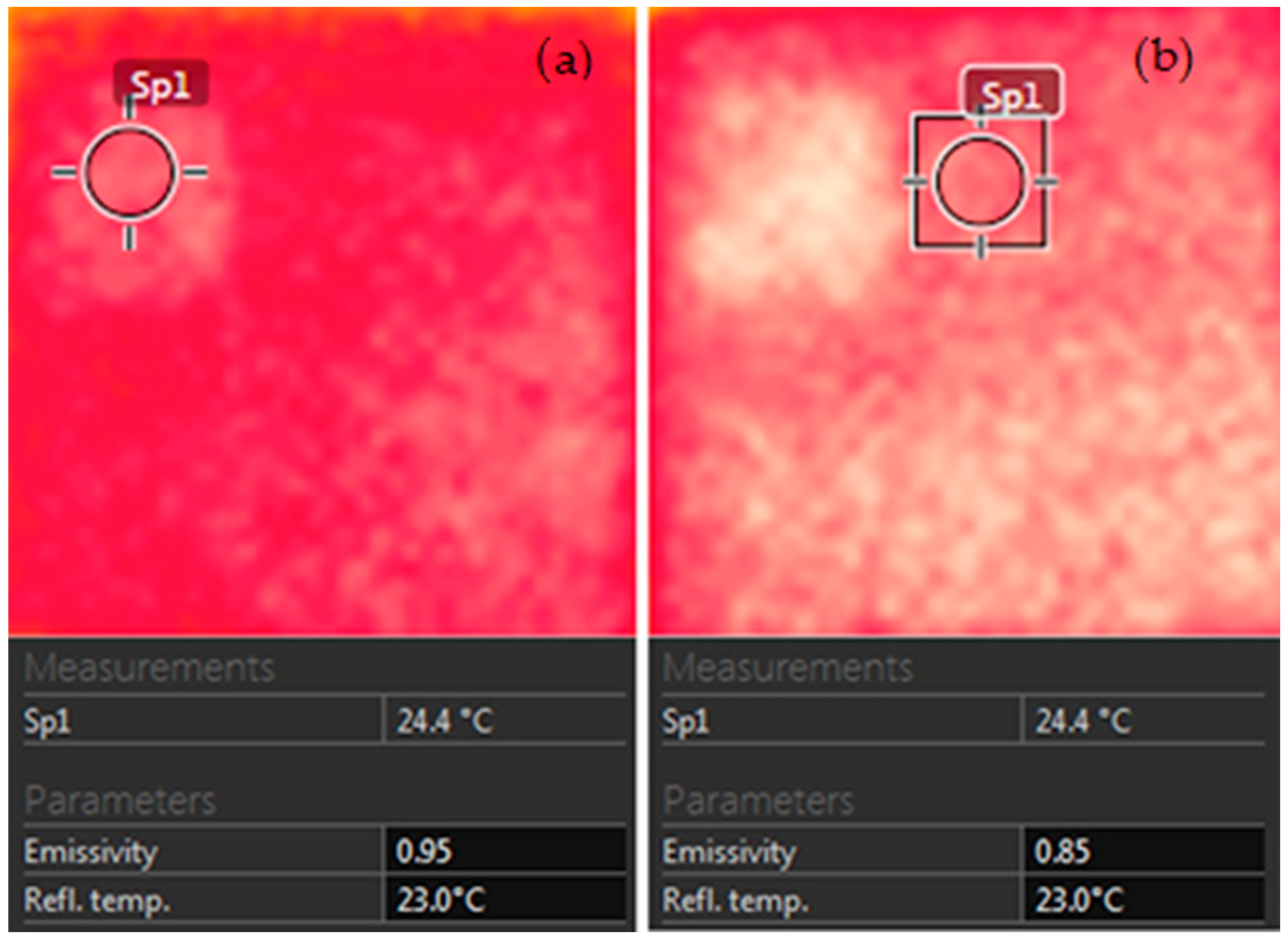
The emissivity was measured using two focus points for each sample. The first point was prepared by placing black tape on the surface of the sample. The measurement of temperature on the middle point of this black surface with known emissivity 0.95 [
14] is shown in
Figure 6a. The second point of measurement was placed on the similar position, but on the sample surface. During the image processing of the second image, it was brought to the same level of the temperature by changing emissivity (as shown in
Figure 6b). A value of 0.85 was adopted for the tested paste.
The pictures using the FLIR camera were taken every half an hour in periods of stable temperatures and every 10 min in periods of intensive temperature fluctuation.
Results from the embedded thermo-sensors were plotted in LabVIEW using temperature–time diagrams. Similar diagrams were generated from the test results of the thermal camera images, after the appropriate image analysis.
These diagrams were then analyzed and compared with the setting time results measured on the cement–fly ash paste samples.
2.4. Modelling
Modelling of the diagrams was performed for the periods where intensive temperature change was noted. Since the heating of the samples was faster than the cooling, the asymmetric Gaussian was used to describe the process, defined by the following parameters:
This model was referred to as univariate asymmetric Gaussian by the authors Kato et al. [
22]. This function returns normalized results ranging from 0 to 1. In order to fit the results of the temperature measurements, the parameters
were adopted for every diagram. This necessitated the addition of the additional parameters
A1,
A2,
N1, and
N2 in order to correlate the obtained results with the actual temperature measurements, which is explained in more detail in
Section 3. The adopted model was then
The moment when the temperature began to rise was adopted as t = 0, while the moment when the temperature began to stabilize was taken as final.
4. Discussion
4.1. The Influence of the Fly Ash Addition to the Cement-Based Composites
The mechanical properties of the mortars containing fly ash were improved, reaching 10.1 MPa for flexural strength and 53.3 MPa for compressive strength after 28 days. Both values were higher than the values measured on the pure cement mortar samples. The beginning and the setting time of the paste containing fly ash were prolonged for one and two hours, respectively, when compared to the pure cement paste.
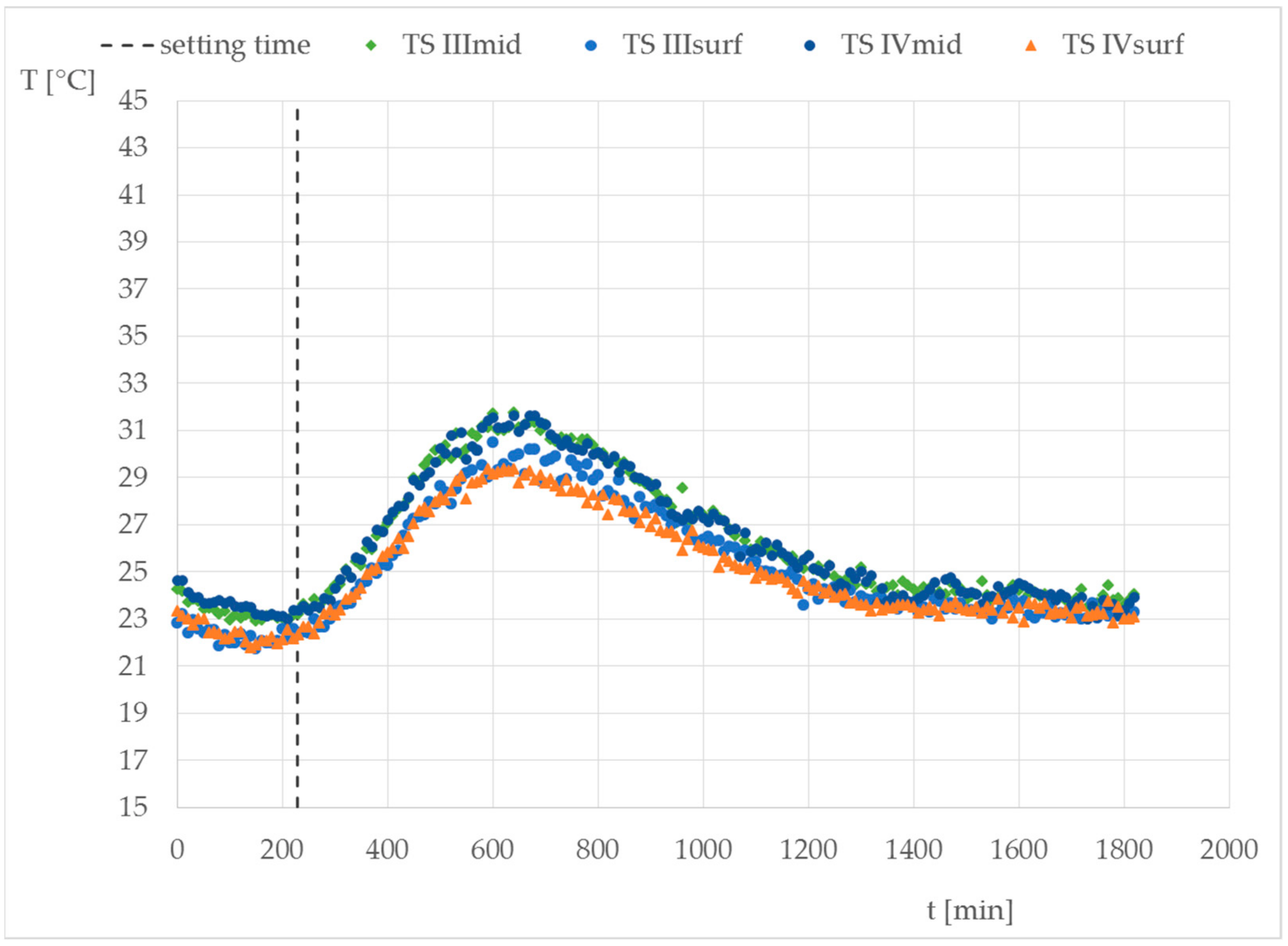
4.2. Temperature Development Discussion
The maximum temperature measured in the central point of the samples was 44 °C, while the maximum temperature on the surface of the samples was 40 °C. These temperatures were measured for the paste in which 20% of cement was replaced with fly ash. The maximum temperature for the paste containing 40% FA (as measured by Zhang et al. [
9]) was 37 °C. The difference was expected due to the larger amount of fly ash used in this study.
If the stages in the temperature development are to be compared to the stages defined in Almattarneh et al. [
11], very good compliance can be observed as well. The first stage in the temperature measurements was approximately 200 min (3.3 h), while the second stage lasted until the maximum temperature was reached, lasting for approximately 7.5 h. The third, cooling stage, lasted for approximately 9 h, which was all in accordance with Almattarneh et al. [
11].
According to the aforementioned, it can be concluded that the obtained results show very good compliance with the results presented in the literature.
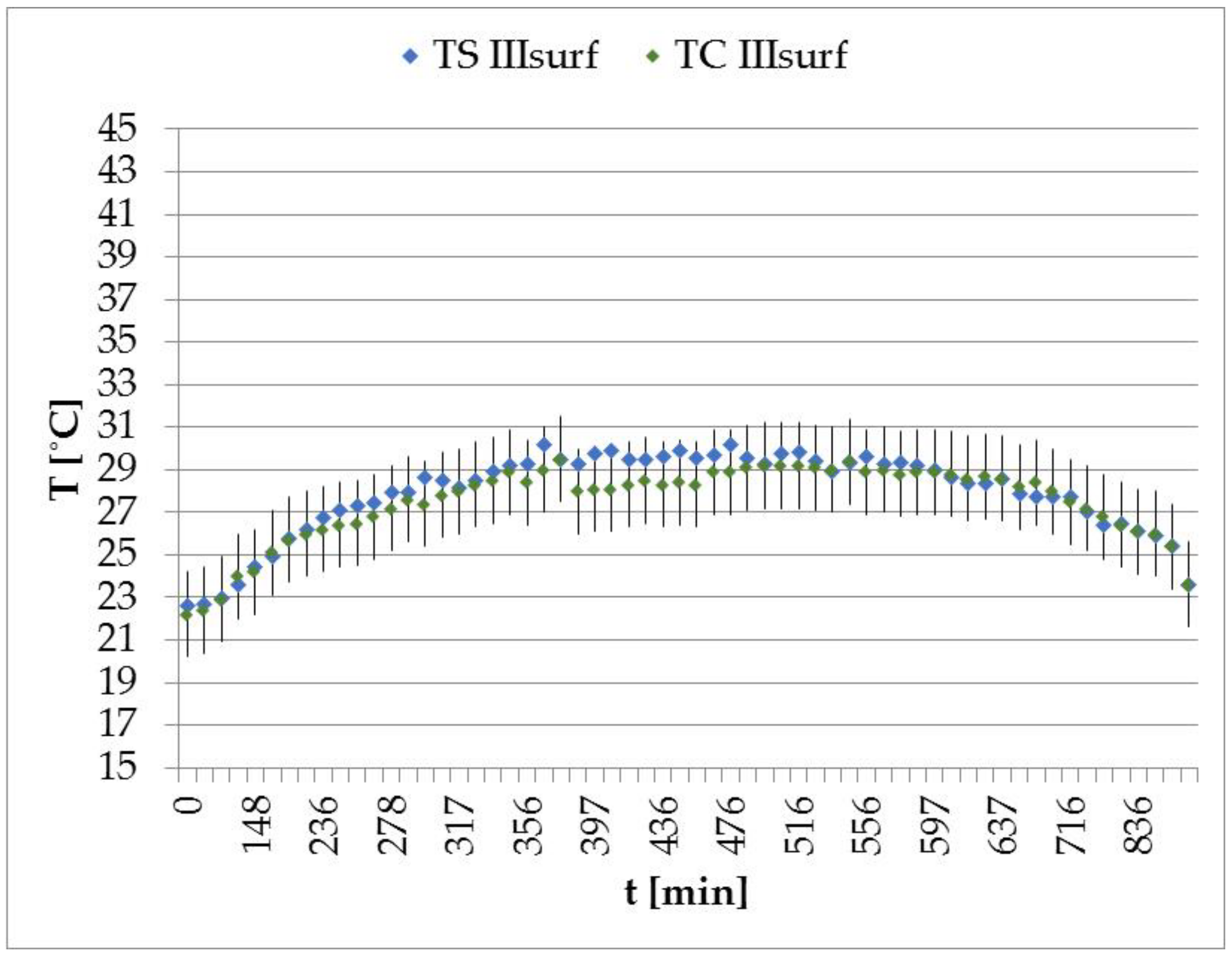
4.3. Comparison between the Results Obtained by Thermal Camera and Thermo-Sensors
The values obtained from the sensor placed in the central part of the samples were expectedly higher than the temperatures measured through sensors placed on the surface or with the thermal camera. The temperatures measured on the surface with two different devices showed very good accordance.
Figure 14 and
Figure 15 represent the results of thermal camera measurements ±2 °C in the central point of the sample and the surface thermal sensors measurements for samples I and III.
As shown in
Figure 14, the highest differences between the measurements occurred in the period of rising temperature and during the temperature peak. Even in this period, the difference was under 2 °C, considered to be the accuracy of the thermal camera measurements. The differences were even smaller for sample III. In conclusion, very good accordance was achieved between the two measuring techniques.
The time when the maximum temperature was reached in the thermal camera recordings slightly differed from the time measured by sensors, but only for the 10 cm high samples.
4.4. Modelling Discussion
All the measurements were modelled through the asymmetric Gaussian function, with very similar coefficients. Small differences between coefficients
A1 and
A2 probably occurred due to the imprecisions in the emissivity measurements, which will be improved through further investigations. The values adopted for the coefficients
ri and
σi were probably in correlation with the specific heat of the cement paste, which was measured in the literature to be 0.736 J/gK for pastes containing larger amounts of water and using only cement as a binder [
13].
For future research, it would be of great importance to perform similar measurements on concrete cubic samples, where the higher heterogeneity of the material could open more interesting questions. Finally, full-scale in situ tests should be performed using the results obtained through the testing of the concrete slabs, bridges, etc.
5. Conclusions
The main focus of the experimental work presented in this paper was the possibility of applying infrared thermography to describe the effects of the temperature development during the early hydration phase of the cement composites. In order to achieve this, a special testing setup was developed and used for temperature measurements in the sample middle point and on the central point of the exposed surface.
The following conclusions were drawn:
The partial replacement of the cement with 20% of fly ash prolonged the setting time of the paste, increased the amount of water necessary for obtaining standard consistency, and increased the flexural and compressive strength of the mortars prepared with these materials.
The results obtained through the system of embedded sensors were very uniform and in accordance with the results found in the literature. As expected, the highest temperatures were measured in the central point of the samples.
Infrared thermography results are comparable with results measured through the embedded thermo-sensors, especially at the surface of the samples.
Although additional confirmatory measurements are necessary, infrared thermography shows the potential to replace embedded sensors on the testing surface of the sample. As noted in the literature, the amount of data collected through the infrared thermography method is greater than by any other method, and its potential is still to be investigated. Further research is necessary to obtain a reliable relation between the inner temperature of the sample and infrared-thermography-based surface measurements.


