Dynamic Mechanical Strength Prediction of BFRC Based on Stacking Ensemble Learning and Genetic Algorithm Optimization

Abstract

Split Hopkinson pressure bar (SHPB) tests are usually used to determine the dynamic mechanical strength of basalt-fiber-reinforced concrete (BFRC), but this test method is time-consuming and expensive. This paper makes predictions about the dynamic mechanical strength of BFRC by employing machine learning (ML) algorithms and feature sets drawn from experimental data from prior works. However, there is still the problem of improving the accuracy of the dynamic mechanical strength prediction by the BFRC, which remains a challenge. Using stacking ensemble learning and genetic algorithms (GA) to optimize parameters, this study proposes a prediction method that combines these two techniques for obtaining accurate predictions. This method is composed of three parts: (1) the training uses multiple base learners, and the algorithms employed by the learners include extreme gradient boosting (XGBoost), gradient boosting (GB), random forest (RF), and support vector regression (SVR); (2) multi-base learners are combined using a stacking strategy to obtain the final prediction; and (3) using GA, the parameters are optimized in the prediction model. An experiment was conducted to compare the proposed approach with popular techniques for machine learning. In the study, the stacking ensemble algorithm integrated the base learner prediction results to improve the model’s performance and the GA further improved prediction accuracy. As a result of the application of the method, the dynamic mechanical strength of BFRC can be predicted with high accuracy. A SHAP analysis was also conducted using the stacking model to determine how important the contributing properties are and the sensitivity of the stacking model. Based on the results of this study, it was found that in the SHPB test, the strain rate had the most significant influence on the DIF, followed by the specimen diameter and the compressive strength.

1. Introduction

Concrete structures are subjected to many different types of loads over the course of their service life, including static loads (such as gravity), but also dynamic loads (such as explosions and impacts) [1,2,3]. The brittleness of concrete, however, under impact loading, can also lead to serious safety problems due to its low cracking resistance; this brittleness increases with an increase in strain rate; concrete’s brittleness can lead to a serious safety problem [4,5]. Due to its strong tensile strength, temperature resistance, and durability, BFRC is widely used in construction [6,7,8]. Additionally, by incorporating basalt fibers (BF) into concrete, the brittleness of concrete can be significantly reduced and the concrete’s impact resistance at high strain rates can be improved significantly [9,10,11].

As terrorist activities increase around the world, there is a growing need to build structures that can withstand blasts to be able to resist these attacks. Xu et al. [12] reported that fiber-reinforced concrete (FRC) has been used as an impact-resistant material for decades and can resist shrinkage and cracking better than plain concrete (PC), since the addition of fibers to FRC results in very different properties in terms of dynamic mechanical properties than those of PC. The determination of the properties of FRC corresponding to different strain rates is therefore critical [13]. There are a wide variety of tests that can be used to study the dynamic properties of BFRC, such as the drop hammer test, the SHPB test, and the air gun test. The SHPB test is one of the most used tests to understand the behavior of a material under different strain rates. A stress–strain curve, a strain rate–time curve, and a stress–time curve of concrete are obtained by measuring the dynamic properties of the curves for the long incidence and transmission bars in the SHPB test.

Currently, to determine the dynamic mechanical strength of BFRC, pie-type specimens of BFRC are usually fabricated. The specimens are subjected to SHPB tests so that stress–strain curves can be generated at different strain rates to collect test data. In general, the method of directly testing BFRC for dynamic mechanical strength will provide more accurate results than a method using estimated predictions. There are, however, other factors affecting BFRC’s dynamic mechanical properties than its strain rate in the SHPB test, including its BF content and length–diameter ratio. It is also worth pointing out that cement manufacturing is one of the major sources of greenhouse gas emissions in the world and poses a serious threat to the environment as a whole [14]. With ML methods, it is possible to achieve accurate predictions of the dynamic mechanical properties of BFRC, so that the problem of over-experimentation in the test process is avoided [15]. By reducing the cost of experiments and reducing CO₂ emissions at the same time, we can protect the environment and reduce costs.

ML methods have become increasingly important in predicting the mechanical properties of building materials to avoid costly experiments. When it comes to training complex models in a highly accurate manner, ML techniques are powerful tools [16,17]. Using an RF algorithm, Hong et al. [18] predicted the compressive strength (CS) of basalt fiber concrete. They found that the model fit well with the experimental data. Mousavi et al. [19] used six ML algorithms to classify wood types, states, and grain orientations. These algorithms included decision trees (DT), support vector machines (SVM), naive Bayes classifiers, nearest-neighbor classifiers, discriminant analysis, and ensemble classifiers. Their results show that different features can provide a better understanding of the problem and that the techniques can be applied to the assessment of wood quality. As part of the freeze–thaw prediction of aggregate by Kahraman et al. [20], gaussian process regression (GPR-Exponential and GPR-Matern5/2), SVM, and regression trees (RT) were applied. In their study, ML techniques were successfully applied to freeze–thaw resistance prediction. Tran [21] used a vast number of proposed ML algorithms to estimate the coefficient of chloride diffusion of concrete. Based on the results, they found that the GB model was the best at predicting the chloride diffusion coefficient with the highest performance. Shamsabadi et al. [22] considered the limitations of ML in the development of the compression strength model of waste marble powder concrete and thoroughly appraised the application of machine learning in this respect. With XGBoost and artificial neural network (ANN) informational models, the CS of WMP concrete could be predicted with high accuracy. Kang et al. [23] developed and compared ML models to predict the CS and flexural strength of steel-fiber-reinforced concrete. According to their research, no matter what the ML algorithm is, the prediction of CS is better than that of bending strength. A new algorithm, FDNN (forest deep neural network), has been proposed by Altayeb et al. [24], which performs better than previous algorithms. Armaghani et al. [25] explored the utilization of artificial intelligence as a viable method for determining the CS of concrete prepared with metakaolin. A neural network model they developed is believed to be the best prediction technology for solving the mortar CS problem. The CS of ground granulated blast furnace slag concrete (GGBFS) was studied and measured by Ahmed et al. [26] using various modeling techniques.

There are several deficiencies in some existing concrete strength prediction studies: (1) few studies have been conducted on the prediction of the mechanical properties, including base strength and dynamic strength, of BFRC; (2) single models are usually chosen in the selection of algorithms, rather than trying to construct new kinds of stacking ensemble models that make use of complementarity between the algorithms; and (3) most existing studies fail to examine the choice of multiple parameters through optimization when constructing prediction models and fail to take into account the significant impact of parameter selection on model accuracy.

In light of the above observations, our study has the following aims: (1) using experimental data from the relevant literature, a comprehensive BFRC dynamic mechanical property prediction dataset will be constructed based on SHPB experiments; (2) an advanced stacking ensemble algorithm will be developed and validated to predict the BFRC dynamic increase factor (DIF) accurately; (3) the optimization problem of determining the key parameters of the model will be solved, and the actual performance of the optimization result verified experimentally; and (4) to elucidate the model and its sensitivity to input variables, as well as to identify the crucial factors influencing the dynamic mechanical performance of BFRC, we will conduct a characteristic importance analysis using SHAP on the input variables. The flow chart of the study is shown in Figure 1.

This study aims to develop a systematic method for dynamic mechanical strength prediction of BFRC and to combine ML methods and intelligent optimization algorithms to build accurate prediction models that can be used to predict the mechanical strengths of BFRC under dynamic conditions. Furthermore, it can be used to build related prediction models in other fields as a reference for building similar models.

2. Data Preprocessing

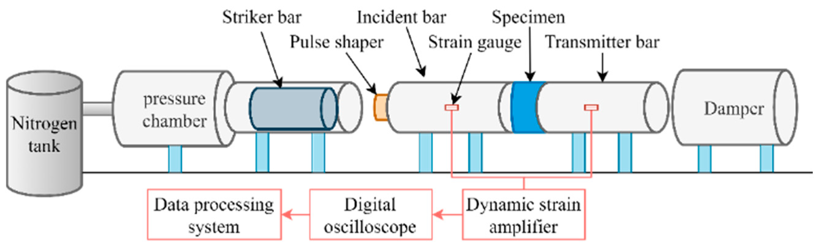
2.1. Experimental Dataset

Currently, SHPB devices are widely used to solve various problems, such as dynamic compression problems, tension, torsion, and triaxial compression. The experimental data from SHPB devices are reliable, and they are easy to use. SHPB devices mainly consist of a firing system, a pressure bar system, a data acquisition system, and a data processing system, as shown in Figure 2. The SHPB test can obtain the dynamic mechanical response of the material under high-speed deformation. Data on the incident pulse (${\epsilon }_i$), the reflected pulse (${\epsilon }_r$), and the drive pulse (${\epsilon }_t$) are collected during the test using strain gauges positioned on the incident bar and the drive bar, respectively. According to the one-dimensional stress wave theory, the plane section assumption and the stress uniformity assumption, the strain (${\epsilon }_s$), stress (${\sigma }_s$) and strain rate ($\dot{\epsilon }$) values were calculated by Equation (1) as follows [27].

$$\begin{array}{c}\left\{\begin{array}{l}{\sigma }_s=E\frac{A}{2A_s}({\epsilon }_i+{\epsilon }_r+{\epsilon }_t)\\ {\epsilon }_s={\int }_0^l\frac{c_0}{l_s}\left({\epsilon }_i-{\epsilon }_r-{\epsilon }_t\right)dt\\ \dot{\epsilon }=\frac{c_0}{l_s}({\epsilon }_i-{\epsilon }_r-{\epsilon }_t)\end{array}\right.\end{array}$$

(1)

where E, A, and $c_0$ represent the elastic modulus (MPa), cross-sectional area (${\mathrm{m}}^2$), and pulse speed ($\mathrm{m}/\mathrm{s}$) of the rod, respectively; and $l_s$ and $A_s$ represent the original length ($\mathrm{m}$) and cross-sectional area (${\mathrm{m}}^2$) of the specimen, respectively.

In this study, the dynamic increase factor (DIF) from impact testing on BFRC using SHPB devices is taken into consideration. DIF is the ratio of the dynamic compressive strength to the quasistatic compressive strength of concrete, as shown in Equation (2). It is often used to describe the effect of strain rate on the mechanical properties of concrete materials [28,29].

$$\begin{array}{c}\mathrm{DIF}=\frac{f_{c,d}}{f_{c,s}}\end{array}$$

(2)

where $f_{c,d}$ is the dynamic compressive strength and $f_{c,s}$ is the quasistatic compressive strength.

Test data for this article were contributed by several BFRC dissertations [30,31,32,33,34,35]. It was decided to utilize only specimens tested at 28 days, since many concrete standards focus on strength. Numerous parameters relating to the mechanical properties and mix design of BFRC were included in this dataset. The parameters in the database were water–cement ratio (W/C), fly ash–cement ratio (F/C), coarse aggregate (CA), fine aggregate (FA), superplasticizer–cement ratio (S/C), length–diameter ratio (FL/FD), fiber content (FC), CS, strain rate (SR), and specimen diameter (SD). Finally, the mechanical properties recorded in the dataset were DIF. The dataset contained eleven parameters divided into ten features and one target. Descriptive statistics for the datasets used in the model development are presented in

Table 1. Descriptive statistics of the dataset used in the development of models.

	W/C	F/C	CA	FA	S/C	FL/FD	FC	CS	SR	SD	DIF
unit	-	-	kg/m3	kg/m3	%	103	%	MPa	/s	mm	-
mean	0.438	0.107	1126	681.8	0.725	0.699	0.416	42.63	183.1	78.33	1.854
std	0.0563	0.106	107	101.3	0.371	0.314	0.608	12.93	164.8	13.95	0.594
min	0.302	0	891	518.3	0	0.2	0	22.29	21	54	0.78
max	0.485	0.25	1368	800	1.301	1.2	2	73.6	796	96	3.582
count	205	205	205	205	205	205	205	205	205	205	205

.

In many cases where the min DIF < 1, the specimens were composed of plain concrete (PC). The phenomenon of lower dynamic compressive strength of plain concrete compared to its static counterpart can be attributed to the impact of strain rate. Under high strain rates, the stress–strain relationship of concrete undergoes a marked transformation. Insufficient time is afforded to energy dissipation mechanisms, such as crack formation and propagation, causing fewer and larger cracks to bear the brunt of the load. This, in turn, leads to reduced strength of the material. At the same time, BFRCs with excessive BF doping exhibit a reduction in strength due to the negative impact of excess BF. This excess BF content can lead to a DIF value of less than 1, indicating a decrease in dynamic mechanical strength.

The specifics of the pairing matrix are illustrated in Figure 3 as variations in the magnitude of each variable’s correlation with the other variables. The value of DIF tends to decrease concerning increases in CA, FL/FD, and CS. The value of DIF rose following the increases in W/C, FA, S/C, FC, and SR. There was no significant impact from some of the other parameters on the DIF.

The coefficient matrix can also yield conclusions comparable to those presented here (Figure 4). CA, FL/FD, and CS all exhibited a negative correlation with CS, with corresponding correlation values of −0.3, −0.42, and −0.52. The degree of the positive correlation among W/C, FA, S/C, FC, SR, and DIF was comparable to 0.45, 0.59, 0.58, 0.55, and 0.54, respectively.

2.2. Data Scaling and Splitting

The dataset using the train_test_split function in Sklearn was randomly divided into two sets: the training set and the test set, in the ratio of 7:3. Models were trained on training sets, and test sets were used to compare predictions with the trained models. The random_state parameter of the train_test_split function was adjusted to 1 for the model with the same objective of ensuring consistency, stability, and reproducibility.

Oey et al. [36] explained that scaling training and test sets before segmentation might cause data leakage. After splitting the training and test sets, we used the RobustScaler function in Sklearn to scale the data. The robustness of the model could be improved by scaling utilizing the median and quartile moments to minimize the effect that outliers had on the model and make the prediction more accurate.

3. Method

3.1. Overview of Stacking Ensemble Algorithm

The stacking model is a hierarchical model ensemble framework where a new regressor combines several individual base learning predictions to predict the target variable [37]. The stacking model usually contains basic models and the meta-learner. The basic models rely on different kinds of algorithms to learn from the original dataset and produce the meta-feature dataset. The meta-learner applies the meta-feature dataset to learn each base model’s strengths and flaws and logically blends their predictions to generate the best performance. K-fold cross-validation is frequently used throughout the training phase of a single basic model to prevent overfitting and guarantee that all original data sets participate in the generation of a new meta-feature dataset. The training process of a single basic model and the structure of the entire stacking model are shown in Figure 5.

3.2. Overview of Genetic Algorithm (GA)

Genetic algorithm (GA) originated from computer simulation studies performed on biological systems. Using Darwin’s theory of evolution and Mendel’s theory of genetics, it is a stochastic global search and optimization method developed to mimic biological evolutionary mechanisms. The method is an efficient, parallel, global search method that discovers the best solution to the problem based on knowledge of the search space acquired automatically during the search process. The fitness function values are used by GA to determine which chromosomes or samples are the best [38]. As determined by the evaluation function, a higher fitness value for each chromosome implies a superior algorithm.

Although the ML model performs brilliantly across the board, it has flaws. One of them is that many parameters are adjustable, and the outcomes may differ depending on the settings used. The search time increases exponentially as the number of parameters increases when using a grid search for parameter tuning. Because of its intrinsic parallelism and capacity to execute distributed computations, the genetic algorithm could rapidly search through all the solutions in the solution space without falling into the pitfalls of fast descent of the local optimal solution. As a result, GA performs better than grid search in terms of efficiency and effectiveness, allowing faster optimization of a wider variety of algorithm parameters. In this paper, we utilized GA to refine the model’s parameter-finding procedure. Model issues, such as excessive tuning time and a plethora of parameters, can be addressed with this method.

3.3. Overview of Random Forest (RF)

RF is an integrated learning algorithm that reduces the fluctuations of a single decision tree by constructing an ensemble of decision trees [39]. By using the concept of “bagging”, many similar data sets randomly selected from the training set are aggregated to create a forest [40]. The bagging algorithm is a parallel algorithm that uses randomly selected training data with put-backs and constructs a classifier; the results are then combined and output. So that nodes are randomly picked with enough features, the RF algorithm optimizes them based on bagging. A suitable feature is obtained from randomly picked sample features for the decision tree’s left and right subtree divisions. They lessen the decision tree’s instability and improve its generalization capabilities. Figure 6 shows the schematic diagram of the bagging algorithm.

3.4. Overview of Gradient Boosting (GB) and Extreme Gradient Boosting (XGBoost)

Figure 7 shows a schematic diagram of the boosting algorithm. By combining several weak learners and increasing the sample weights for the subsequent model depending on the learning from the prior model, the boosting method creates strong learners [41]. As a result, each subsequent learning outcome is influenced by the preceding one, and the amount of decision trees increases the weight of the data. In the boosting algorithm, the model is constructed by iterating in steps, and weak learners are built to compensate for weaknesses in the existing model during each iteration [42].

GB is an integrated algorithm based on decision trees, which is one of the boosting algorithms that are effective in data analysis and prediction. GB uses the residual from each round as input and tries to fit this residual into the next round’s output so that the residual keeps getting smaller as the training continues. With each weak learner training round, GB changes toward a decreasing gradient of the loss function [43].

XGBoost is an improvement over the boosting algorithm based on the GB. In contrast to GB, XGBoost expands its loss function directly using both first-order and second-order gradients rather than using first-order gradients for its loss function. Thus, XGBoost fits more accurately and faster [44].

In several fields, XGBoost is used since it allows for more significant problem-solving capabilities and fewer usage conditions. Compared to GB, XGBoost also has a shorter learning time and better predictive power when a large amount of data are available. Due to the above, this paper employed the XGBoost algorithm and compared the overall performance of boosting techniques [45,46].

3.5. Overview of Support Vector Regression (SVR)

The SVR algorithm can solve linear and nonlinear regression problems [47]. Pattern recognition and data classification are both possible with this method, and it has a strong generalization ability [48]. By combining a series of kernel functions, SVR constructs a highly reliable regression model for predicting output values. The training sets indicating the coordinates of spatiotemporal points are mapped to a multidimensional feature space using hyperplanes. A further benefit of this approach is that it allows the user to employ the best kernel function for predicting the results.

3.6. Model Development

ML models usually use grid searches for optimal parameter tuning. The grid search will adjust the parameters sequentially in steps within the specified parameter range, train the model with the adjusted parameters, and find the best combination of parameters with the highest cross-validation score on the test set from all the parameter combinations. The advantage of this method is its simplicity and stability. However, the grid search will be time-consuming when the optimal parameter interval cannot be predicted.

To address the problems in the model, this paper uses a GA to optimize the parameter search process of the model and compare it with grid search. Figure 8 shows the schematic diagram of the GA. The basic idea of the optimization is to consider the frequently modified parameters in the ML model as the individual population of the genetic algorithm and to use the final training score of the ML model as the fitness function to search for the optimal parameters and improve the performance of the learner through the process of selection, crossover, and variation.

3.7. Model Evaluation

ML algorithms are evaluated based on mean square error (MSE), root mean square error (RMSE), coefficient of determination ($R^2$), and mean absolute error (MAE). The estimation of regression models in this type of problem relies heavily on these metrics.

In a regression model, $R^2$ is the variance fraction of the response characteristics, and its value can range from negative infinity to 1 [49]. As a result, if the model fits the data exactly, $R^2$ will be assumed to be 1, and the model will explain all the variability in the data [50]. As a result of the enhanced interpretability of the model’s performance, it is also regarded as the standard version of MSE, as shown in Equation (3). The MSE is calculated by averaging the squared differences between the actual and predicted values, as shown in Equation (4). It is the most widely used loss function in regression models. RMSE is equal to the square root of MSE, as shown in Equation (5). Due to the square effect, MSE values are more difficult to interpret than RMSE values, so RMSE is often used to evaluate models. MAE is the mean of absolute errors, as shown in Equation (6). MAE is also known as absolute loss.

$$R^2=1-\frac{\sum _{i=1}^n(y_i-{\widehat{y}}_i{)}^2}{\sum _{i=1}^n(y_i-\overline{y}{)}^2}$$

(3)

$$\mathrm{M}\mathrm{S}\mathrm{E}=\frac{1}{n}\sum _{i=1}^n(y_i-{\widehat{y}}_i{)}^2$$

(4)

$$\mathrm{R}\mathrm{M}\mathrm{S}\mathrm{E}=\sqrt{\frac{1}{n}\sum _{i=1}^n(y_i-{\widehat{y}}_i{)}^2}$$

(5)

$$\mathrm{M}\mathrm{A}\mathrm{E}=\frac{1}{n}\sum _{i=1}^n\left|y_i-{\widehat{y}}_i\right|$$

(6)

where ${\widehat{y}}_i$ is the predicted value, $y_i$ is the actual value, $\overline{y}$ is the sample mean, and $n$ is the number of data samples.

4. Result and Discussion

Five models are considered in this paper: XGBoost, GB, RF, SVR, and stacking models. In the stacking model, XGBoost, GB, and RF are used as basic models, and SVR is used as a meta-learner. This section illustrates the performance of the models in terms of different methods of parameter optimization, comparison of models, and the feature importance of the models.

4.1. Comparison of Different Ways of Parameters Optimization

The parameter optimization via grid search and GA for models is shown in

Table 2. The parameters of ML models.

ML Models	Parameters	Grid Search	GA
XGBoost	N-estimators	100	223
	Learning-rate	0.1	0.41
	Max-depth	3	2
	Min-child-weight	1	10
	Gamma	1	0.07
	Subsample	1	0.95
	Colsample-bytree	1	0.98
GB	N-estimators	100	230
	Learning-rate	0.15	0.53
	Max-depth	2	9
	Min-samples-leaf	0	10
	Alpha	0.9	0.79
	Subsample	1	0.71
RF	N-estimators	100	103
	Max-depth	6	8
SVR	C	10	178.73
	Gamma	0.1	0.1

. The default settings for the other models’ parameters are used. The optimization process of the GA is expounded in Section 3.6. In view of the copious number of iterations, which typically surpass 100 generations, and the fact that the iterative process solely presents the current optimal training score and ultimate parameter settings, the intricate details of the iterative optimization process are intentionally omitted.

The performance of the algorithms after grid search and GA tuning parameters is shown in Figure 9. The $R^2$ of the five algorithms is shown in Figure 9a. The $R^2$ of the training set for all models with parameter tuning was higher than that of the test set. In addition, the $R^2$ of the test set for the models with parameter tuning by GA was higher than that of the grid search. Among all the models, the model using SVR had the largest $R^2$ improvement after adjusting the parameters using GA. At the same time, the value of MAE, MSE, and RMSE also decreased the most (Figure 9b–d). This means that the model with GA tuning can further improve the performance, which is consistent with the performance comparison of other models. Like the case of $R^2$, the performance of the test part of all algorithms is always weaker than the training part. The stacking model parametrized by GA had the best performance with the highest $R^2$ and the lowest value of MAE, MSE, and RMSE. Overall, the model’s predictive performance was enhanced when parameters were optimized via GA as opposed to grid search.

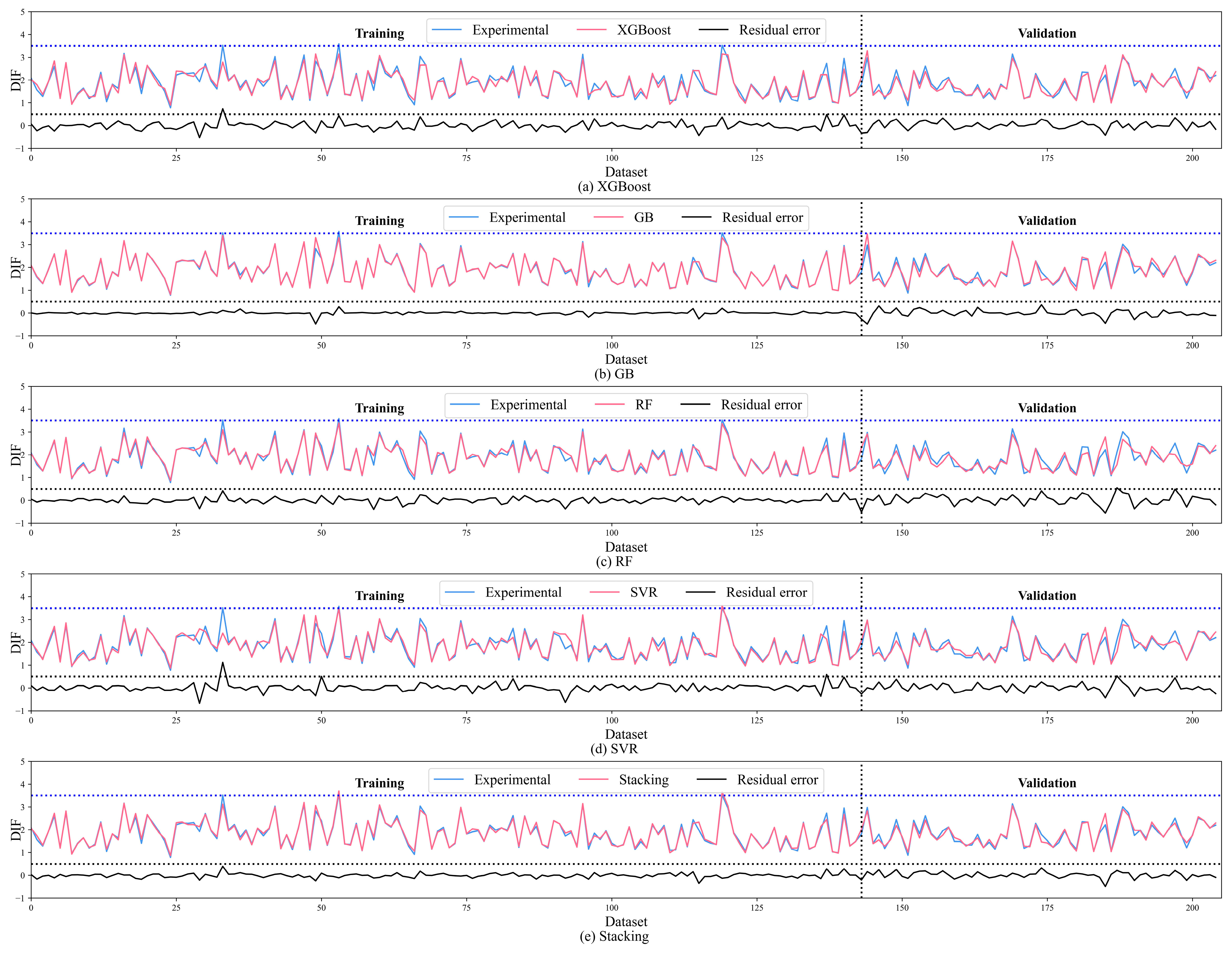
4.2. Comparison and Evaluation of Five Model

Figure 10 gives the predicted DIF of BFRC obtained by the five algorithms after optimizing the parameters using GA. In each diagram, the blue line depicts the actual DIF from the experiment, while the red line shows the DIF prediction from the ML algorithm. Additionally, the error for each sample is shown by the black line in each diagram. It was found that for most samples in the training set, the deviation between the predicted and actual values was relatively small, which indicates the good performance of the trained model. The larger deviations between the predicted and actual values in the test set compared to the training set can be seen in Figure 10. Among them, the RF model (Figure 10c) had the largest error fluctuation, and the stacking model (Figure 10e) had the smallest error fluctuation. The analysis’ findings demonstrate that the stacking model makes the most accurate predictions.

It can be seen from

Table 3. DIF prediction results from machine learning models based on GA parameter optimization.

ML Models	Training				Testing
	R2	MAE	MSE	RMSE	R2	MAE	MSE	RMSE
XGBoost	0.9261	0.1203	0.0286	0.1692	0.9035	0.1263	0.0258	0.1608
GB	0.9877	0.0349	0.0048	0.0691	0.9143	0.106	0.023	0.1515
RF	0.963	0.0848	0.0143	0.1198	0.8189	0.1708	0.0485	0.2203
SVM	0.9111	0.1219	0.0345	0.1857	0.8825	0.1329	0.0315	0.1774
Stacking	0.9769	0.0669	0.0089	0.0946	0.9326	0.1007	0.0181	0.1344

that performance indices values ($R^2$, MAE, MSE, RMSE) values are determined for the DIF in the case of the five models based on GA parameter optimization for the training and validation datasets. The fitness of the model is characterized by $R^2$. The $R^2$ of XGBoost, GB, and stacking models in this study were above 0.9 for both training and test sets, indicating their high accuracy. The $R^2$ deviation between the training and test sets of the RF model was relatively large, indicating that the generalization ability of the RF model was weaker than the other models. The stacking model achieved the largest $R^2$ value among all models on the training set (0.9326), which indicates that the stacking model has the best generalization ability and the best ability to fit the data compared to the other models. MSE and RMSE are commonly used to describe the degree of variability of the data, and MAE can reflect the true picture of the prediction error. The reduced values of these indices depict the higher performance of both models. From Table 3, the values of MAE, MSE, and RMSE for the RF model were the highest. This means that the RF model has the lowest accuracy, while the other models have relatively high accuracy. Meanwhile, the values of MAE, MSE, and RMSE of the stacking model on the test set were 0.93, 0.1007, 0.0181, and 0.1344, respectively. These values were the smallest compared to the other models. This indicates that the accuracy of stacking is the highest and the error is the lowest. Therefore, the stacking model based on GA optimization parameters proposed in this paper has higher accuracy and generalization ability.

Figure 11 and Figure 12 depict the predicted-to-experimental ratio widely used as a statistical evaluation for a model [51,52,53]. It can be noted that for the training and validation data of the stacking model, 121/142 (85.2%) and 45/64 (70.3%) of the predictions were recorded within ±5% of the relative error. Similarly, the XGBoost model interpreted 93/142 (65.5%) and 32/64 (50%) of the predicted values as ±5% of the relative error. The GB model interpreted 134/142 (94.4%) and 36/64 (56.3%) of the predicted values as ±5% of the relative error. The RF model interpreted 114/142 (80.3%) and 36/64 (56.3%) of the predicted values as ±5% of the relative error. The SVR model interpreted 98/142 (69%) and 45/64 (70.3%) of the predicted values as ±5% of the relative error. The stacking model had a higher error accuracy of the predicted values in the training set with the highest error accuracy in the test set, proving its superiority in predicting the DIF of BFRC.

4.3. Sensitivity Analysis Using SHAP

As part of designing the BFRC, it is crucial to analyze the effect of input variables on the DIF of the BFRC. A sensitivity analysis of the model is necessary to understand the stability of the algorithm. Additionally, the stacking ensemble algorithm should be detailed to understand how the predicted DIF is analyzed and calculated. Hence, the ability of SHAP to explain the ML model is based on ideas derived from game theory [54]. The shapely value approach describes a way to evaluate each input variable’s relative influence and contribution to the final output variable, represented by a shapely plot. This approach entails holding all other variables constant while changing one to determine the impact of a change in one variable on the target attribute.

The SHAP, based on game theoretical ideas, is a method of calculating the SHAP values which measures the contribution of each input variable to a model’s prediction by considering all possible combinations and splits of these variables. The formula for this method, as shown in Equation (7), represents a significant step towards understanding the underlying mechanisms of ML models and the interpretation of their results.

$$\begin{array}{c}g\left(x^{\prime }\right)={\phi }_0+\sum _{j=1}^M{\phi }_j{x}_j^{\prime }=f\left(x\right)\end{array}$$

(7)

where $g\left(x^{\prime }\right)$ is the explained model, $f\left(x\right)$ is the ML algorithm, $x^{\prime }$ is the simplified input and takes the value of 1 (same value of the feature) or 0 (loss of values of features), ${\phi }_0$ is the predicted mean value of the machine learning algorithm on the dataset, ${\phi }_j$ is the contribution value of the feature (i.e., SHAP value), and $M$ is the total number of features.

Figure 13 presents the calculation schematic of SHAP, which allows for a comprehensive evaluation of the contribution of each variable to the prediction results, accounting for both individual variables and their interactions. Using SHAP techniques, a more nuanced understanding of machine learning models can be gained, enabling their more effective application and improvement. By elucidating the role and significance of each variable in the model, we provide an intuitive reference for the preparation of BFRC and the sensitivity of the model to input variables.

Figure 14 shows the importance of the input variables in demonstrating the impact of the imputed characteristics on the prediction of the target variables. The results here are calculated by averaging the shapely values over the entire data set. As can be seen from the figure, SR is the most important variable affecting the DIF. This is consistent with the actual knowledge of concrete. The second important variable is SD, which is due to the size effect of the specimens. CS is the third important input variable. From this figure, we can also see that W/C is the least important variable. The observed discrepancy between our findings and the current understanding of concrete behavior may be attributed to the limited range of water–cement ratios covered in our dataset.

Figure 15 shows the global interpretation of the GB model by SHAP interpretation, showing the trend of the corresponding variables and the distribution of SHAP values for individual features. The X-axis indicates the SHAP values of the ten input features. Positive and negative SHAP values indicate the positive and negative gain of the DIF. Red dots indicate high feature values of the sample and blue dots indicate low feature values of the sample. From Figure 15, for SR, samples with higher values have positive SHAP values, which means that higher SR is beneficial for DIF. SD samples with higher values have positive SHAP values, indicating that an appropriate increase in specimen size can improve the DIF of BFRC. In a reversal of the observed trend for the SD samples, individuals with high sample values in the CS samples exhibited negative SHAP values, implying that a greater DIF was observed in BFRC with lower compressive strengths. Since summary plots summarize the relative importance of the input factors and how they relate to the independent variable, they play a crucial role in SHAP analysis.

5. Conclusions

In this paper, a stacking ensemble model combining XGBoost, GB, RF, and SVR models is proposed to predict the dynamic increase factor of BFRC, and all the parameters of the model are optimized using GA. The main conclusions are as follows:

(1)

In comparison to grid search, the performance of the model is improved when the parameters are optimized via GA. The performance of the algorithm can be improved by simultaneously optimizing more parameters with GA.

(2)

The stacking ensemble model presented in this research allows distinct prediction models to learn from one another by observing data space and structure from diverse angles. Predicted to experimental ratio also showed the stacking ensemble model’s advantage.

(3)

The SHAP analysis validated the developed stacking model and showed that the strain rate of the SHPB test was the most influential variable on the DIF values, followed by the specimen diameter and the compressive strength.

The results show that the model combines a strong predictive capability and a low correlation base learner with good prediction accuracy and high application value. Thus, the stacking ensemble model has high prediction accuracy and stability with several application values as follows:

(1)

It guides the dynamic mechanical strength calculation of BFRC required for engineering.

(2)

It effectively reduces the difficulty of obtaining the dynamic mechanical strength of BFRC, reduces the workload of conducting experiments, and is more economical and environmentally friendly.

Some of the contributions made by this study are as follows:

(1)

A dynamic mechanical property performance prediction dataset was developed based on the SHPB experiments.

(2)

A stacking ensemble model for predicting the DIF of BFRC was proposed based on the superposition algorithm; in this model, XGBoost, GB, and RF are used as basic models and SVR is used as a meta-learner.

(3)

We developed a GA for parameter optimization to determine the key parameters for the prediction model.

(4)

To evaluate the effectiveness of the proposed method, extensive numerical experiments were conducted on the collected data and results showing that the proposed method performs better than popular machine learning algorithms, including SVR, RF, GB, and XGBoost.

(5)

According to the SHAP and feature importance analyses, the strain rate of the SHPB test influenced the DIF most, followed by the specimen diameter and the compressive strength.

6. Limitations and Future Work

In the quest to accurately predict the dynamic increase factor of BFRC, existing experimental records from various sources were utilized in this study. However, due to the limited availability of experimental data, the range of some features, such as water-to-cement ratio, only ranged from 0.302 to 0.485, which can lead to a decrease in the model’s generalization ability. To establish a more accurate model, extensive experimental testing must be carried out under controlled conditions, and data must be collected from a single source with known environmental conditions.

Through the analysis of the input variables in the model, it was revealed that these variables can be optimized through feature engineering and quantitative simplification. Notably, the impact of CA and FA on the predictive power of the model is not obvious when considered as individual variables. Thus, combining the two into a single variable for input, i.e., F/C, is a promising strategy to reduce the number of input variables and improve the model’s generalization performance. Moreover, this approach can help to uncover the hidden relationship between FA and CA, providing valuable insights into the composition of BFRC.

To enhance the predictive performance of the model, we proposed investigating other ML models, including light GBM and DNN, optimized using genetic algorithms. These models can be incorporated into the stacking ensemble model to improve the accuracy of the dynamic increase factor prediction model. These findings shed light on the potential of utilizing machine learning algorithms and the importance of extensive experimental testing in accurately predicting the mechanical strength of BFRC, as well as other fiber-reinforced concrete materials. We hope that these findings will inspire more research into the optimization of machine learning algorithms for predicting the mechanical properties of composite materials.

References

1. Xiao, S.-H.; Liao, S.-J.; Zhong, G.-Q.; Guo, Y.-C.; Lin, J.-X.; Xie, Z.-H.; Song, Y. Dynamic properties of PVA short fiber reinforced low-calcium fly ash—Slag geopolymer under an SHPB impact load. J. Build. Eng. 2021, 44, 103220. [Google Scholar] [CrossRef]
2. Li, L.; Wang, H.; Wu, J.; Du, X.; Zhang, X.; Yao, Y. Experimental and numerical investigation on impact dynamic performance of steel fiber reinforced concrete beams at elevated temperatures. J. Build. Eng. 2022, 47, 103841. [Google Scholar] [CrossRef]
3. Sica, S.; Pagano, L.; Rotili, F. Rapid drawdown on earth dam stability after a strong earthquake. Comput. Geotech. 2019, 116, 103187. [Google Scholar] [CrossRef]
4. Hao, Y.F.; Hao, H.; Jiang, G.P.; Zhou, Y. Experimental confirmation of some factors influencing dynamic concrete compressive strengths in high-speed impact tests. Cem. Concr. Res. 2013, 52, 63–70. [Google Scholar] [CrossRef]
5. Zhang, X.; Elazim, A.A.; Ruiz, G.; Yu, R. Fracture behaviour of steel fibre-reinforced concrete at a wide range of loading rates. Int. J. Impact Eng. 2014, 71, 89–96. [Google Scholar] [CrossRef]
6. Branston, J.; Das, S.; Kenno, S.Y.; Taylor, C. Mechanical behaviour of basalt fibre reinforced concrete. Constr. Build. Mater. 2016, 124, 878–886. [Google Scholar] [CrossRef]
7. Jiang, C.; Fan, K.; Wu, F.; Chen, D. Experimental study on the mechanical properties and microstructure of chopped basalt fibre reinforced concrete. Mater. Des. 2014, 58, 187–193. [Google Scholar] [CrossRef]
8. Sim, J.; Park, C.; Moon, D.Y. Characteristics of basalt fiber as a strengthening material for concrete structures. Compos. Part B Eng. 2005, 36, 504–512. [Google Scholar] [CrossRef]
9. Wu, Z.; Shi, C.; He, W.; Wang, D. Static and dynamic compressive properties of ultra-high performance concrete (UHPC) with hybrid steel fiber reinforcements. Cem. Concr. Compos. 2017, 79, 148–157. [Google Scholar] [CrossRef]
10. Lai, J.; Sun, W. Dynamic behaviour and visco-elastic damage model of ultra-high performance cementitious composite. Cem. Concr. Res. 2009, 39, 1044–1051. [Google Scholar] [CrossRef]
11. Mastali, M.; Dalvand, A.; Sattarifard, A. The impact resistance and mechanical properties of reinforced self-compacting concrete with recycled glass fibre reinforced polymers. J. Clean. Prod. 2016, 124, 312–324. [Google Scholar] [CrossRef]
12. Xu, Z.; Hao, H.; Li, H. Experimental study of dynamic compressive properties of fibre reinforced concrete material with dif-ferent fibres. Mater. Des. 2012, 33, 42–55. [Google Scholar] [CrossRef]
13. Yoo, D.-Y.; Banthia, N. Impact resistance of fiber-reinforced concrete—A review. Cem. Concr. Compos. 2019, 104, 103389. [Google Scholar] [CrossRef]
14. Ghosh, S.; Dinda, S.; Das Chatterjee, N.; Dutta, S.; Bera, D. Spatial-explicit carbon emission-sequestration balance estimation and evaluation of emission susceptible zones in an Eastern Himalayan city using Pressure-Sensitivity-Resilience framework: An approach towards achieving low carbon cities. J. Clean. Prod. 2022, 336, 130417. [Google Scholar] [CrossRef]
15. Li, H.; Lin, J.; Zhao, D.; Shi, G.; Wu, H.; Wei, T.; Li, D.; Zhang, J. A BFRC compressive strength prediction method via kernel extreme learning machine-genetic algorithm. Constr. Build. Mater. 2022, 344, 128076. [Google Scholar] [CrossRef]
16. Murphy, K.P. Machine Learning: A Probabilistic Perspective; MIT Press: Cambridge, MA, USA, 2012. [Google Scholar]
17. DeRousseau, M.; Kasprzyk, J.; Srubar, W. Computational design optimization of concrete mixtures: A review. Cem. Concr. Res. 2018, 109, 42–53. [Google Scholar] [CrossRef]
18. Li, H.; Lin, J.; Lei, X.; Wei, T. Compressive strength prediction of basalt fiber reinforced concrete via random forest algorithm. Mater. Today Commun. 2022, 30, 103117. [Google Scholar] [CrossRef]
19. Mousavi, M.; Gandomi, A.H.; Holloway, D.; Berry, A.; Chen, F. Machine learning analysis of features extracted from time–frequency domain of ultrasonic testing results for wood material assessment. Constr. Build. Mater. 2022, 342, 127761. [Google Scholar] [CrossRef]
20. Kahraman, E.; Ozdemir, A.C. The prediction of durability to freeze–thaw of limestone aggregates using machine-learning techniques. Constr. Build. Mater. 2022, 324, 126678. [Google Scholar] [CrossRef]
21. Tran, V.Q. Machine learning approach for investigating chloride diffusion coefficient of concrete containing supplementary cementitious materials. Constr. Build. Mater. 2022, 328, 127103. [Google Scholar] [CrossRef]
22. Shamsabadi, E.A.; Roshan, N.; Hadigheh, S.A.; Nehdi, M.L.; Khodabakhshian, A.; Ghalehnovi, M. Machine learning-based compressive strength modelling of concrete incorporating waste marble powder. Constr. Build. Mater. 2022, 324, 126592. [Google Scholar] [CrossRef]
23. Kang, M.C.; Yoo, D.Y.; Gupta, R. Machine learning-based prediction for compressive and flexural strengths of steel fi-ber-reinforced concrete. Constr. Build. Mater. 2021, 266, 121117. [Google Scholar] [CrossRef]
24. Altayeb, M.; Wang, X.; Musa, T.H. An ensemble method for predicting the mechanical properties of strain hardening ce-mentitious composites. Constr. Build. Mater. 2021, 286, 122807. [Google Scholar] [CrossRef]
25. Armaghani, D.J.; Asteris, P.G. A comparative study of ANN and ANFIS models for the prediction of cement-based mortar materials compressive strength. Neural Comput. Appl. 2021, 33, 4501–4532. [Google Scholar] [CrossRef]
26. Ahmed, H.U.; Mostafa, R.R.; Mohammed, A.; Sihag, P.; Qadir, A. Support vector regression (SVR) and grey wolf optimization (GWO) to predict the compressive strength of GGBFS-based geopolymer concrete. Neural Comput. Appl. 2022, 35, 2909–2926. [Google Scholar] [CrossRef]
27. Zhang, H.; Wang, L.; Zheng, K.; Bakura, T.J.; Jibrin, T.; Totakhil, P.G. Research on compressive impact dynamic behavior and constitutive model of polypropylene fiber reinforced concrete. Constr. Build. Mater. 2018, 187, 584–595. [Google Scholar] [CrossRef]
28. Li, N.; Jin, Z.; Long, G.; Chen, L.; Fu, Q.; Yu, Y.; Zhang, X.; Xiong, C. Impact resistance of steel fiber-reinforced self-compacting concrete (SCC) at high strain rates. J. Build. Eng. 2021, 38, 102212. [Google Scholar] [CrossRef]
29. Su, H.; Xu, J.; Ren, W. Mechanical properties of geopolymer concrete exposed to dynamic compression under elevated tem-peratures. Ceram. Int. 2016, 42, 3888–3898. [Google Scholar] [CrossRef]
30. Shen, L.; Xu, J.; Li, W.; Fan, F.; Yang, J. Experimental investigation on the static and dynamic behaviour of Basalt fibres reinforced concrete. Concrete 2008, 4, 026. [Google Scholar]
31. Zhang, H.; Wang, B.; Xie, A.; Qi, Y. Experimental study on dynamic mechanical properties and constitutive model of basalt fiber reinforced concrete. Constr. Build. Mater. 2017, 152, 154–167. [Google Scholar] [CrossRef]
32. Pengfei, C. Research and Numerical Analysis on Impact Resistance of Basalt Fiber and Polypropylene Fiber Reinforced Concrete; Qingdao Technological University: Qingdao, China, 2021. [Google Scholar]
33. Ganorkar, K.; Goel, M.D.; Chakraborty, T. Specimen Size Effect and Dynamic Increase Factor for Basalt Fiber–Reinforced Concrete Using Split Hopkinson Pressure Bar. J. Mater. Civ. Eng. 2021, 33, 04021364. [Google Scholar] [CrossRef]
34. Xu, J.; Fan, F.; Bai, E.; Liu, J. Study on dynamic mechanical properties of basalt fibre reinforced concrete. Chin. J. Undergr. Space Eng. 2010, 6, 1665–1671. [Google Scholar]
35. Xie, L.; Sun, X.; Yu, Z.; Guan, Z.; Long, A.; Lian, H.; Lian, Y. Experimental study and theoretical analysis on dynamic mechanical properties of basalt fiber reinforced concrete. J. Build. Eng. 2022, 62, 105334. [Google Scholar] [CrossRef]
36. Oey, T.; Jones, S.; Bullard, J.W.; Sant, G. Machine learning can predict setting behavior and strength evolution of hydrating cement systems. J. Am. Ceram. Soc. 2019, 103, 480–490. [Google Scholar] [CrossRef]
37. Wolpert, D.H. Stacked generalization. Neural Netw. 1992, 5, 241–259. [Google Scholar] [CrossRef]
38. Jiang, Y.; Tong, G.; Yin, H.; Xiong, N. A Pedestrian Detection Method Based on Genetic Algorithm for Optimize XGBoost Training Parameters. IEEE Access 2019, 7, 118310–118321. [Google Scholar] [CrossRef]
39. Fawagreh, K.; Gaber, M.M.; Elyan, E. Random forests: From early developments to recent advancements. Syst. Sci. Control Eng. Open Access J. 2014, 2, 602–609. [Google Scholar] [CrossRef]
40. Breiman, L. Bagging predictors. Mach. Learn. 1996, 24, 123–140. [Google Scholar] [CrossRef]
41. Freund, Y.; Schapire, R.E. A Decision-Theoretic Generalization of On-Line Learning and an Application to Boosting. J. Comput. Syst. Sci. 1997, 55, 119–139. [Google Scholar] [CrossRef]
42. Hastie, T.; Friedman, J.H.; Tibshirani, R. The Elements of Statistical Learning: Data Mining, Inference, and Prediction; Springer: New York, NY, USA, 2009; Volume 1, Issue 3; pp. 267–268. [Google Scholar]
43. Friedman, J.H. Greedy function approximation: A gradient boosting machine. Ann. Stat. 2001, 29, 1189–1232. [Google Scholar] [CrossRef]
44. Sun, J.; Zhang, J.; Gu, Y.; Huang, Y.; Sun, Y.; Ma, G. Prediction of permeability and unconfined compressive strength of pervious concrete using evolved support vector regression. Constr. Build. Mater. 2019, 207, 440–449. [Google Scholar] [CrossRef]
45. Duan, J.; Asteris, P.G.; Nguyen, H.; Bui, X.-N.; Moayedi, H. A novel artificial intelligence technique to predict compressive strength of recycled aggregate concrete using ICA-XGBoost model. Eng. Comput. 2021, 37, 3329–3346. [Google Scholar] [CrossRef]
46. Chen, T.; Guestrin, C. Xgboost: A scalable tree boosting system. In Proceedings of the 22nd ACM SIGKDD International Conference on Knowledge Discovery and Data Mining; ACM: New York, NY, USA, 2016; pp. 785–794. [Google Scholar]
47. Friedman, J.H. Stochastic gradient boosting. Comput. Stat. Data Anal. 2002, 38, 367–378. [Google Scholar] [CrossRef]
48. Yuvaraj, P.; Murthy, A.R.; Iyer, N.R.; Sekar, S.; Samui, P. Support vector regression based models to predict fracture characteristics of high strength and ultra high strength concrete beams. Eng. Fract. Mech. 2013, 98, 29–43. [Google Scholar] [CrossRef]
49. DeRousseau, M.; Laftchiev, E.; Kasprzyk, J.R.; Rajagopalan, B.; Srubar, W.V., III. A comparison of machine learning methods for predicting the compressive strength of field-placed concrete. Constr. Build. Mater. 2019, 228, 116661. [Google Scholar] [CrossRef]
50. Cameron, A.C.; Windmeijer, F.A.G. An R-squared measure of goodness of fit for some common nonlinear regression models. J. Econ. 1997, 77, 329–342. [Google Scholar] [CrossRef]
51. Feng, D.-C.; Wang, W.-J.; Mangalathu, S.; Taciroglu, E. Interpretable XGBoost-SHAP Machine-Learning Model for Shear Strength Prediction of Squat RC Walls. J. Struct. Eng. 2021, 147, 04021173. [Google Scholar] [CrossRef]
52. Amin, M.N.; Iqbal, M.; Jamal, A.; Ullah, S.; Khan, K.; Abu-Arab, A.M.; Al-Ahmad, Q.M.S.; Khan, S. GEP Tree-Based Prediction Model for Interfacial Bond Strength of Externally Bonded FRP Laminates on Grooves with Concrete Prism. Polymers 2022, 14, 2016. [Google Scholar] [CrossRef]
53. Alabdullah, A.A.; Iqbal, M.; Zahid, M.; Khan, K.; Amin, M.N.; Jalal, F.E. Prediction of rapid chloride penetration resistance of metakaolin based high strength concrete using light GBM and XGBoost models by incorporating SHAP analysis. Constr. Build. Mater. 2022, 345, 128296. [Google Scholar] [CrossRef]
54. Lundberg, S.M.; Lee, S.-I. A unified approach to interpreting model predictions. In Proceedings of the Advances in Neural Information Processing Systems, Long Beach, CA, USA, 4–9 December 2017; Volume 30. [Google Scholar]
Figure 1. Research flow chart.
Buildings 13 01155 g001
Figure 2. SHPB equipment and schematic diagram.
Buildings 13 01155 g002
Figure 3. Pair diagrams showing variations of magnitudes of variables with each other.
Buildings 13 01155 g003
Figure 4. Correlation coefficients matrix.
Buildings 13 01155 g004
Figure 5. Illustration of stacking ensemble algorithm.
Buildings 13 01155 g005
Figure 6. Illustration of bagging method.
Buildings 13 01155 g006
Figure 7. Illustration of boosting method.
Buildings 13 01155 g007
Figure 8. Schematic diagram of the GA.
Buildings 13 01155 g008
Figure 9. Performance of the algorithms after grid search and GA tuning parameters.
Buildings 13 01155 g009
Figure 10. Comparison of DIF prediction with various algorithms.
Buildings 13 01155 g010
Figure 11. Predicted/experimental ratio (training set).
Buildings 13 01155 g011
Figure 12. Predicted/experimental ratio (testing set).
Buildings 13 01155 g012
Figure 13. SHAP analysis.
Buildings 13 01155 g013
Figure 14. Feature importance.
Buildings 13 01155 g014
Figure 15. SHAP summary plot.
Buildings 13 01155 g015