Non-Destructive Damage Detection of Structural Joint by Coaxial Correlation Method in 6D Space

Abstract

Failure of joints can lead to structural collapse. It is vital to monitor joint stiffness during operation to prevent such failures. This paper proposes a novel method for the quality assessment of structural joints using coaxial correlation in 6D space. Coaxially placed 6D sensors on either side of the joint implemented by 3D accelerometers and 3D gyroscopes with wide frequency range, automatic synchronisation between the input signal and receivers and response signal averaging are presented. The root mean square (RMS) value from the obtained signals convolution is proposed as a measure of the similarity between two signals for monitoring joint degradation. The method’s effectiveness was tested on steel beam splice connection, where it was found that the RMS of convolution signals in 6D space showed a direct correlation between the calculated RMS value in X, Y, GX, and GY axes directions and the stiffness grades of the joint. The paper concludes that the nature of the RMS during the degradation of the joint may change in different axes, and wrongly chosen axes may lead to wrong conclusions regarding the state of the investigated joint, especially in the case of complex joints, so that the measurements in 6D provide higher reliability of the result interpretation.

1. Introduction

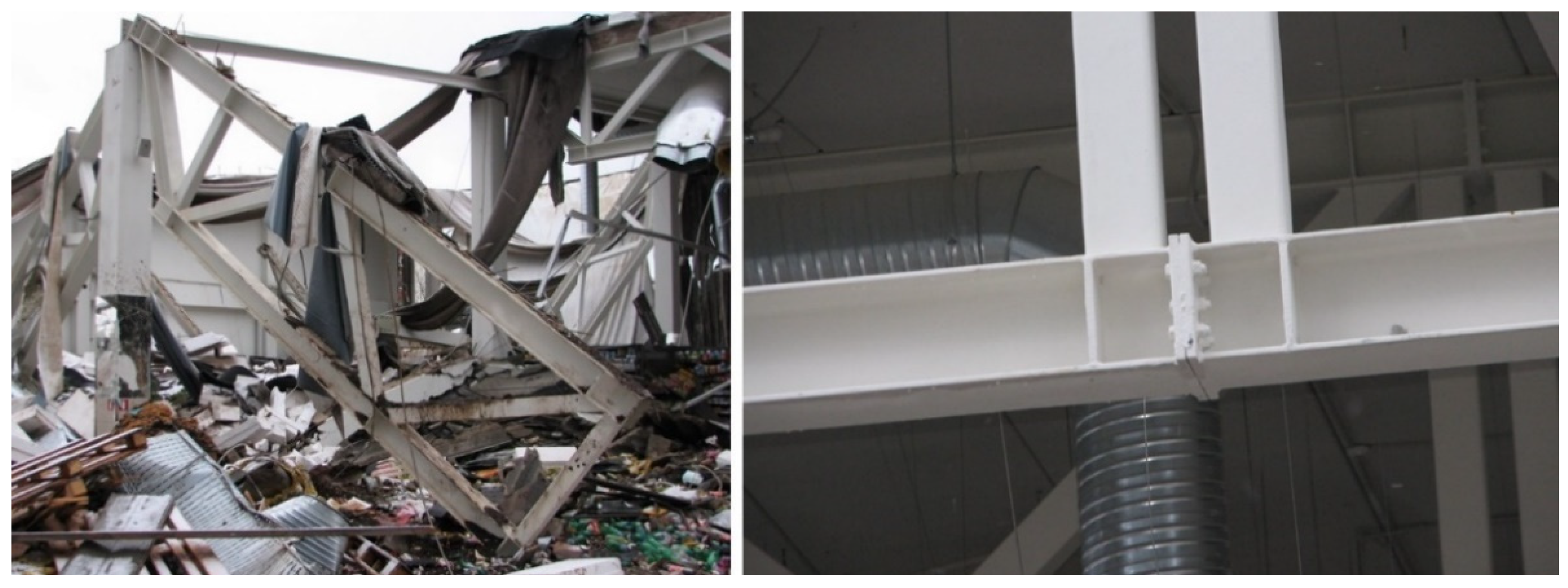
Structural failures in building structures are often attributable to the failure of the structural components connecting the structural elements. Such failures of the structural units can occur due to a loss of strength or buckling of their elements resulting from decreases in their parameters during operation or design errors [1]. One of the most devastating examples of such structural failures is the collapse of the roof of the Maxima shopping centre in Riga, Latvia, in 2013. The cause of the accident was traced back to the failure of the assembly joint of the bottom chord of a trapezoidal steel truss, which served as the main load-bearing structure for the roof. The consequences of the roof collapse and the fault joint leading to the accident are depicted in Figure 1.

This is just one example of the importance of joints and the global impact on the whole structure. Therefore, it is essential to ensure that the joint stiffness corresponds to the designed level during operation [2,3].

A joint’s stiffness directly impacts the distribution of internal forces and deformations within a structure [4]. Joints can be classified as pinned joints, which are a more conservative solution since the beams are designed for higher bending moment values, as the moment is not transmitted through the joint, and moment-resisting joints. Moment-resisting connections are connections between structural members that are designed to transfer bending moment between them. They are commonly used in multi-story buildings, bridges, and industrial facilities where the structure is subject to high horizontal or lateral loads. The design of moment-resisting connections involves ensuring that the connection is strong and stiff enough to transfer the bending moment without excessive deformation or failure. In steel structures, moment-resisting connections are often achieved through the use of welded or bolted connections.

Bolted connections can be designed as moment-resisting connections by using high-strength bolts and plates with sufficient thickness and stiffness to transfer the required bending moment. However, bolted connections generally have lower stiffness and strength compared to welded connections and are more prone to fatigue and failure over time due to cyclic loading [5]. Welded connections, on the other hand, can provide higher stiffness and strength compared to bolted connections, and are often preferred in situations where high loads and bending moments are expected. After the Northridge earthquake in California in 1994, where welded connections showed inadequate performance, bolted connections have been deeply studied [6,7,8], increasing the popularity of combination of welded and bolted moment connections, such as bolted end-plate connection, extended end-plate connection, flange plate moment connections and others, which can offer high ductility with good ability to dissipate energy, which is essential in the case of seismic or cyclic loading, as well as high quality and prompt assembly [6,9].

The inspection and maintenance during steel structures operation is required for the moment-resisting joints as the redistribution of moments decreases as the joint loses its stiffness, leading to higher internal forces and significant second-order effects [10]. Therefore, the moment-resisting joints are of interest for non-destructive testing (NDT) methods and it is essential to check the existing stiffness of the joint and compare it with the initially designed stiffness.

The vibration method is a commonly used non-destructive technique [11]. Vibration-based techniques for identifying damages in joints is a constantly evolving and advancing field, with new methods and technologies being developed and continuously tested.

Generally, the non-destructive quality control vibration method involves three primary stages [12]. The first stage involves applying vibrations to a specimen using special equipment, such as modal impact hammers or advanced shakers, depending on the desired frequency range or ambient vibrations [13,14]. In the second stage, the vibrational response of the specimen is measured using either contact sensors, such as accelerometers [15], or noncontact sensors, such as laser doppler vibrometers. Several emerging technologies, such as fibre-optic sensing and wireless sensor networks, are also being developed to enable real-time monitoring of joint health and detect any changes in its condition [16,17,18,19]. Finally, in the third stage, the obtained data from the second step is processed to identify changes and characterise the system.

There are many different approaches to processing the data obtained. One of the common techniques is the use of frequency response functions (FRFs) to identify changes in the dynamic behaviour of the joint, which can indicate the presence of damage [20,21,22,23]. FRF of a linear mechanical system is defined as the Fourier transform of the time domain response divided by the Fourier transform of the time domain input [24]. Other techniques involve using wavelet transform analysis instead of Fourier analysis, which makes it possible to analyse dynamic behaviour in the signal, so that is a powerful tool for use in artificial intelligence and machine learning algorithms to process vibration signals and identify damage patterns in the joint [25,26]. Another approach involves the estimation of changes in the dynamic properties of the specimen, including vibration frequencies, damping ratios, and modal shapes, by using either experimental modal analysis (EMA) or operational modal analysis (OMA) [22,27,28,29,30].

This paper proposes a novel method for assessing the quality of structural joints using coaxial correlation in 6D space, which involves the use of 6D sensors with a wide frequency range, automatic synchronization, and response signal averaging to measure joint stiffness. The proposed method for quality control of moment-resisting structural joints involves exciting the structure with a known input signal and measuring the structure’s response by using a pair of coaxially positioned sensors. The sensors are symmetrically placed on either side of the joint, aligned with its axis. The post-processing by correlation of obtained measured responses is made to predict the damages in the joint. The proposed method was verified for bolted splice connection between IPE 80 steel beams. It is a commonly used and easily accessible parallel flange I section that allows focusing on the evaluation of joint degradation using a simple, relatively lightweight, and effective moment joint model for the laboratory test. The chosen joint solution is specifically selected because of its simplicity and the ease of simulating the degradation of a moment-resisting joint in laboratory conditions. This is accomplished by reducing the stiffness of the joint through the loosening of bolts. The verification aimed to determine the relationship between the correlation of measured specimen responses and joint stiffness to verify the proposed method’s concept and evaluate its effectiveness for assessing structural moment-resisting joint degradation in steel beams.

2. Materials and Methods

2.1. Improved Coaxial Correlations Method for Structural Joints Quality Evaluation

The proposed method for evaluating the degradation of the structural joint was shown promising results in the case of T-type joints, where two beams are joined at right angles to each other, forming a T-shape, both for timber and steel structures [31,32]. However, the first version of the method for evaluating the quality of structural joints, which involves using an electronic testing system and mathematical analysis of the recorded data, as described in [31,32], also had several shortcomings. For example, there was an insufficient frequency range of the used sensors, the possibility of measurements only in 3D space, inconvenience related to the manual handling of multiple repeated measurements, and the need for strong input signals.

The electronic system’s first improvement involves using 6D sensors implemented by MPU-9250, which contains a 3-axis gyroscope and a 3-axis accelerometer. Three-dimensional gyroscopes consist of three independent vibratory MEMS rate gyroscopes, which detect rotation about the X, Y and Z axes. The analog-to-digital converter (ADC) sample rate for 3D gyroscopes is programmable from 8000 samples per second. The ADC sample rate for 3D accelerometers is 4000 samples per second. The 16-bit resolution of the ADC device has been used, which provides that each sample can take one of 2¹⁶ possible values, ranging from −32,767 to 32,767. The 16-bit resolution of the ADC device allows for a high level of precision in the digital representation of the signal amplitude.

Based on Nyquist theorem [33], also known as the sampling theorem, the sampling frequency must be at least twice the maximum frequency of the original signal to reconstruct an analog signal from its sampled digital representation accurately:

$$f_{\mathrm{sampling}}\ge 2\times f_{\mathrm{input},\max },$$

(1)

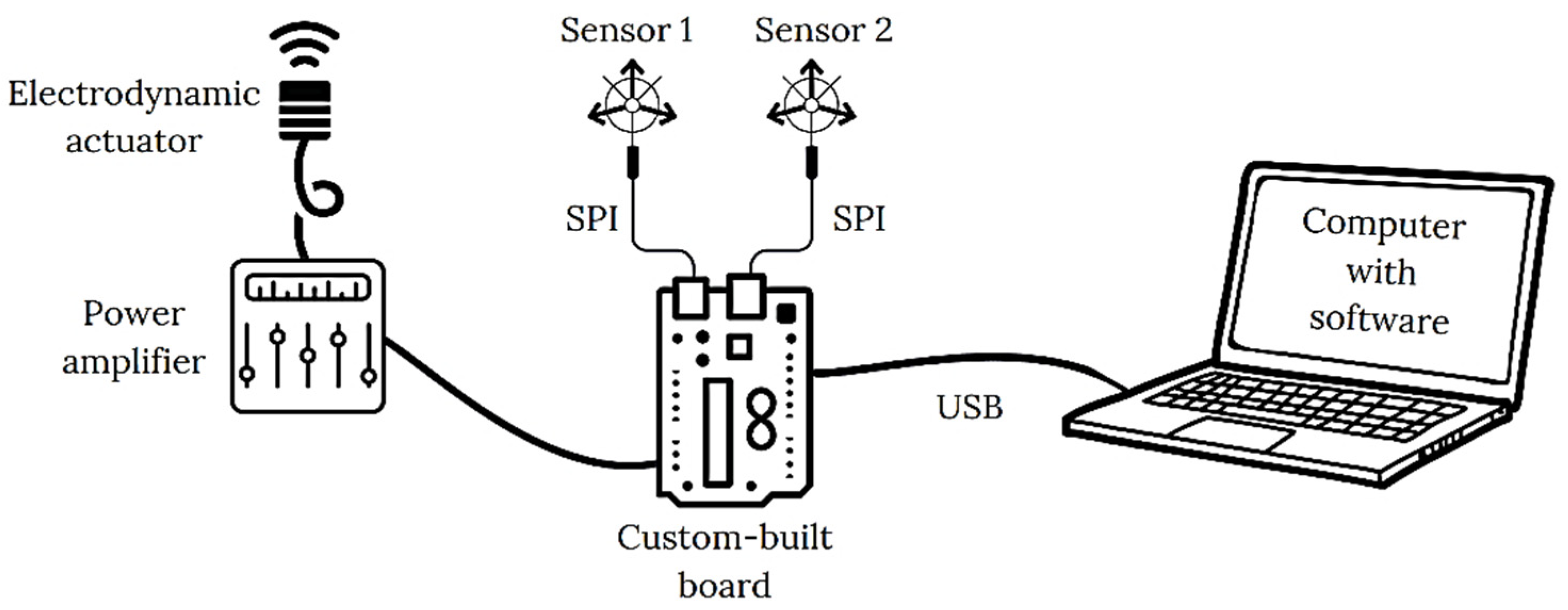
where f_sampling is the ADC sample rate, the number of samples per second; f_input,max is the highest frequency component of the sampled signal. Therefore, the frequency range for 3D accelerometers is 0 Hz to 2000 Hz, and for 3D gyroscopes it is 0 Hz to 4000 Hz. It has been hypothesised that 6D sensors can describe the state of the joint more fully, which would be especially important in the case of complex joints. The second improvement is the introduction of automatic synchronisation between the input signal and the receivers, as well as the use of the averaging method, which made it possible to significantly decrease the influence of the noise in the measurements of the structure’s response and made it possible to use even weak excitation signals for measurements. It is suggested to use at least 16 scans for significant (four times) improvement in the signal-to-noise ratio [34]. The improved electronic testing system is shown in Figure 2.

The enhanced system includes 6D sensors with a wider frequency, and a custom-built board instead of the previously used Arduino board. The custom-built board contains the STM32 microcontroller family based on the ARM Cortex-M processor architecture. These microcontrollers combine high performance, low power consumption, and a wide range of integrated peripherals and features, making them suitable for a wide variety of embedded applications. For a signal generation, Pulse Width Modulation (PWM) with a low pass filter is integrated into the custom-built board. In this way, a powerful technique for controlling the parameters of the generated signal is obtained, as it allows for precise and efficient control. A low-pass filter removes the high-frequency components and smooths out the signal. PWM is a method of controlling the power delivered to a load by modulating the width of a pulse of constant amplitude and frequency. By changing the duty cycle of the pulse, the effective voltage or current delivered to the load can be varied [35,36,37].

An electrodynamic actuator was used to generate an input signal as a short impulse. The electronic system provides measurements taken in six-dimensional space using two 6D sensors, coaxially positioned on the beams on either side of the joint. A crucial aspect in placing the sensors and the electrodynamic actuator is ensuring the sensors’ symmetrical positioning on both sides of the joint and aligned with its axis. Electronic system improvements allowed processing response signals from a wider frequency range and simplified the data collecting process. The impulse is sent many times, and the response data F1 and F2 from the first and second sensors are collected and averaged. Averaged data is saved for further post-processing, and the procedure is repeated for the medicated object of investigation.

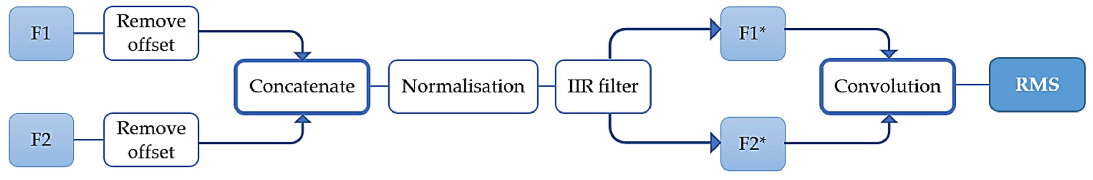
The signal analysis software package with a wide range of powerful tools and statistics functions, SIGVIEW, is used to post-process collected data. The processing of the collected data F1 and F2 in the time domain includes:

• Remove the constant offset from F1 and F2 by subtracting the signal’s mean value from all the amplitude values. The result is a signal with a mean equal to zero;
• Make the normalisation of concatenated pairs of responses F1 and F2 to ensure a mutual comparison of the obtained data under the conditions of the experiment with artificial degradation of the connection;
• Choose the frequency range in which the object’s behaviour under study will be observed based on the spectrum analysis;
• Split the filtered concatenated signal into two signals, F1* and F2*;
• Convolve the obtained normalised pairs of signals F1* and F2* from both sensors to characterise the degree of similarity between the two signals.;
• Determine the root mean square (RMS) value from the obtained signals convolution as a measure of the similarity between two signals.

Schematically, the post-processing process is shown in Figure 3.

The obtained step six parameter RMS is proposed for monitoring the system’s condition during operation as a reference point using determined parameters at the initial stage, with an approved design stiffness condition of the system.

2.2. Verification Approach

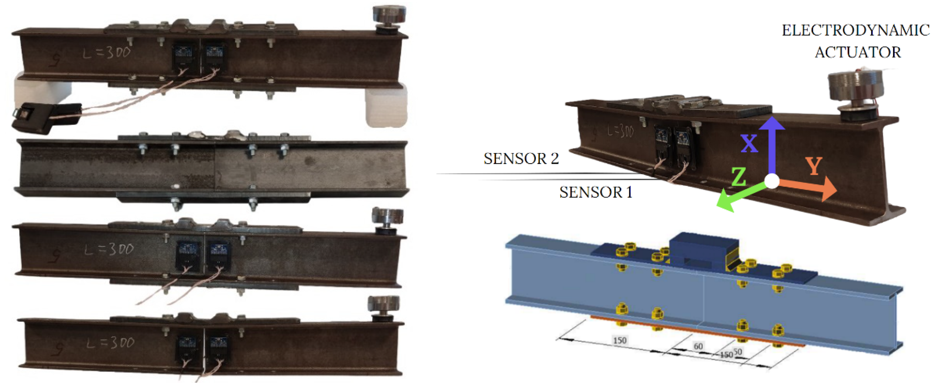
The steel beam specimen with splice connection was prepared (Figure 4) to check the possibility of damage detection of bolted splice connection by coaxial accelerations correlation.

The investigated steel specimen consisted of S355 strength class parallel flange I section IPE 80 steel beam elements with dimensions according EN 10365, where the height is 80 mm, the width is 46 mm, the web thickness is 3.8 mm, the flange thickness is 5.2 mm and the root fillet radius is 5.0 mm. A total length of the specimen is 600 mm that had been halved and joined using two metal plates with dimensions of 46 mm × 300 mm and thicknesses of 8 mm. One metal connector plate is positioned on the top face and the other on the bottom face of the specimen. The connection between the steel beam and steel plates was established using 8.8-grade M8 bolts. The positioning of holes for bolts is adopted following the requirements of the Eurocode EN 1993-1-8 of minimum and maximum spacing and end and edge distances for bolts. Since shear resistance of the bolts is decisive, the distance between the bolts is not essential and is not assumed as a variable for this test. The joint was investigated using varying numbers of bolts—16, 12, 8 and 4. In the case of 4 bolts, the bottom metal connector plate was removed. The degradation of a connection during operation has been artificially characterized by unbolting the bolts and removing the metal connector plate. Structural joint degradation can occur due to factors such as loosening of the bolts and/or corrosion. The order of unbolting was as follows: first, the 4 bottom bolts were unbolted, 2 edge bolts on each side of the joint; second, the 4 top bolts were unbolted, and 2 edge bolts on each side of the joint; finally, the last 4 bottom bolts were unbolted, and the bottom metal plate was removed.

Unbolting bolts allowed adjustments to the joint’s stiffness to be made and analysed using the proposed coaxial correlation method. During the experiment, constant support conditions for the specimen are provided: simply supported (roller-roller) on vibration-absorbing supports with a span of 500 mm.

The structural joint model is created using 3D modelling software Tekla Structures in accordance with the European standard EN 1993-1-8, which outlines the general principles and rules for designing joints in steel structures. Once the joint model is prepared, it is exported from Tekla Structures to IDEA StatiCa and analysed using the finite element analysis (FEA) method.

To accurately model the joint, both the webs and flanges of connected members as well as metal connector plates are modelled using 4-node quadrangle shell elements with nodes at each corner. The size of the finite elements varies from 5 to 10 mm, and the meshing is done automatically. Fasteners, such as bolts, are modelled using special FEM components.

The steel joint is analysed using a nonlinear, elastic-plastic material model. After conducting the calculations, the maximum value of the bending moment that the specimen can withstand is determined. In this case, with all 16 bolts, in a three-point bending configuration, the specimen is treated as a simply supported beam with a span of 500 mm. Based on the calculations, the maximum value of the bending moment that the specimen can absorb is determined to be equal to 4.75 kNm.

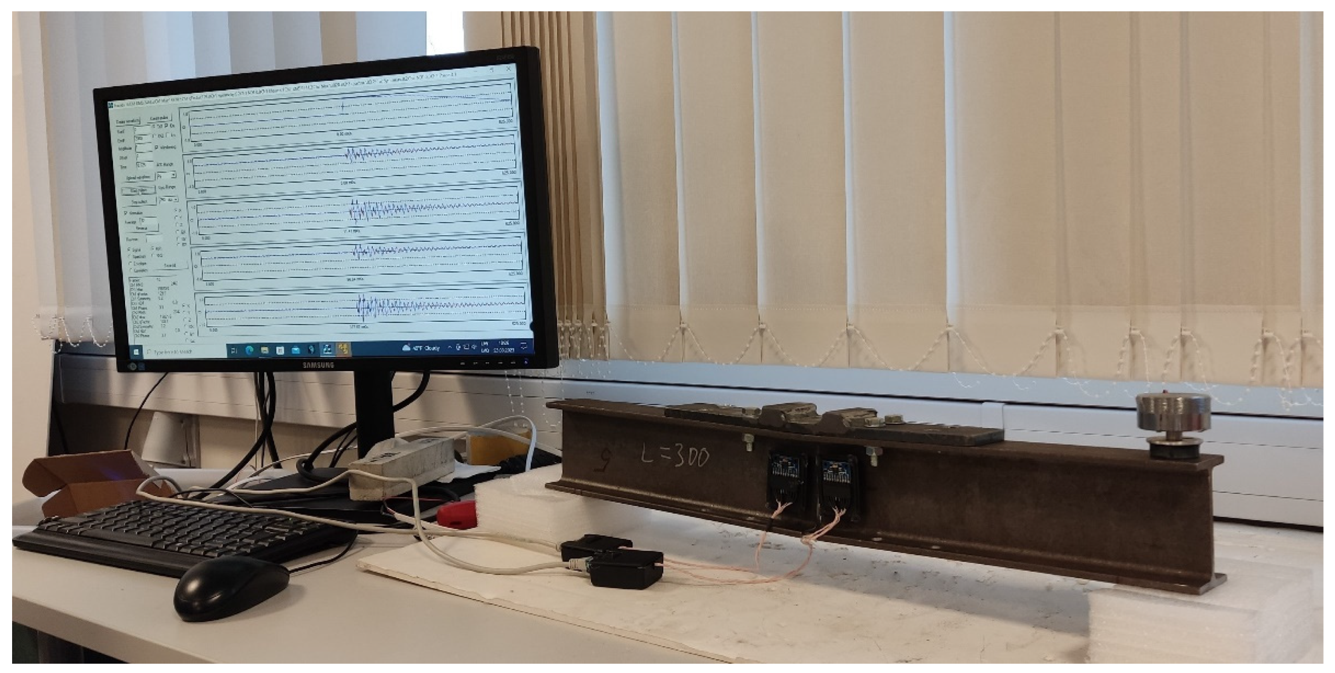
The vibration load was generated by an electrodynamic actuator mounted on one end of the beam coaxially to the X-axis of the specimen. The structure’s response was measured in three directions, namely, X, Y, and Z (see Figure 4), using two 3D accelerometers and around three axes, namely, GX, GY, and GZ, using two 3D gyroscopes, thus providing 6D space measurements. Next, 6D sensors 1 and 2 were coaxially placed on the beams on either side of the beam splice connection. The process of specimen testing is shown in Figure 5. The obtained signals were transmitted to a computer with corresponding software for further processing.

3. Results and Discussion

The vibration tests were conducted to assess the effectiveness of the coaxial acceleration correlation technique in detecting changes in joint stiffness in steel beam splice connections. In order to simulate a reduction in joint stiffness, the bolts were gradually unbolted. These tests aimed to confirm whether the technique could accurately identify variations in joint stiffness. The results of the tests provided valuable insights into the method’s performance and potential applications in structural joints.

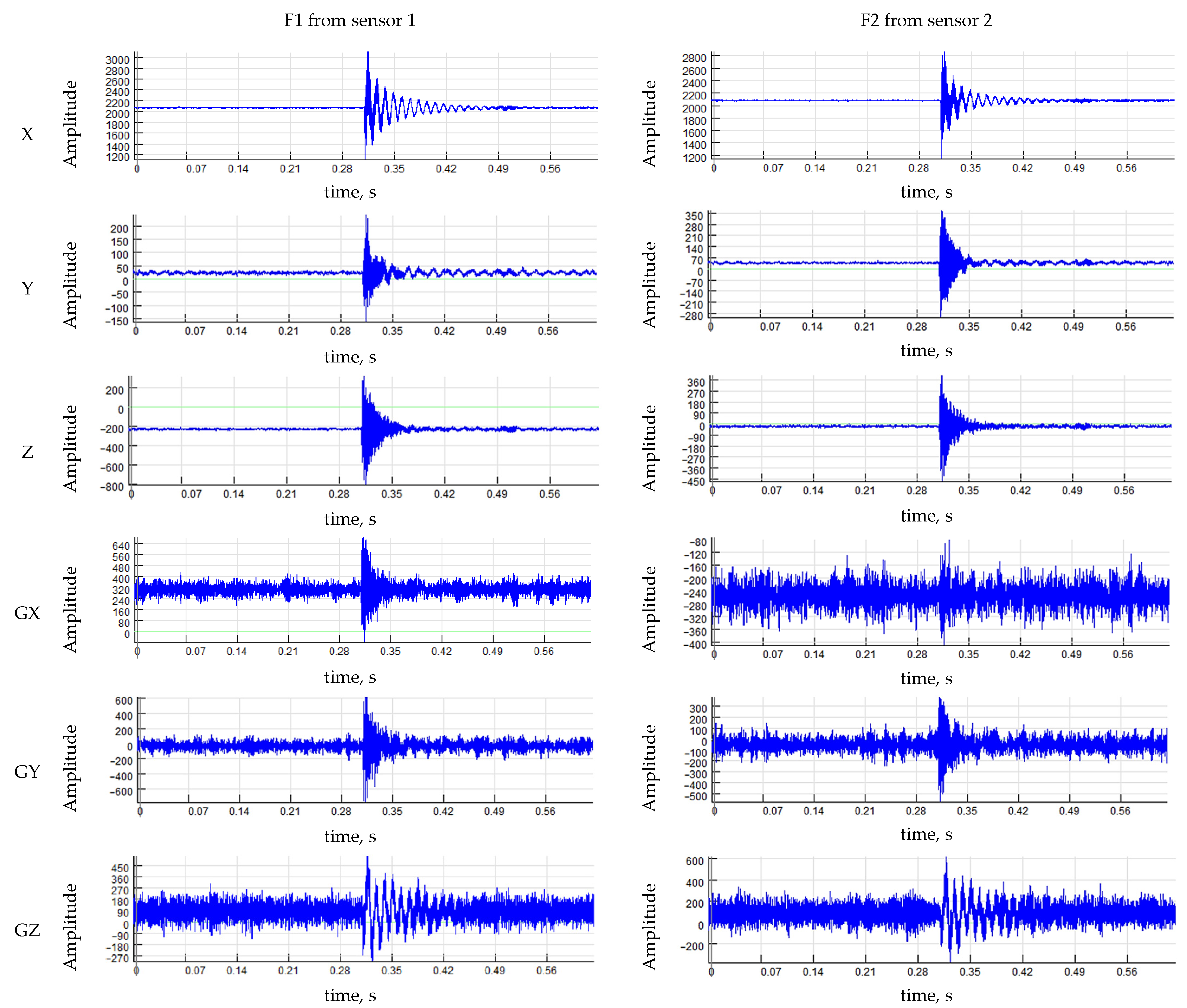
The averaging function was applied to response records from coaxially placed 6D sensors to obtain accurate data. This function helped minimise the effects of external noise or vibration on the measurements. The collected response records in 6 different axes for specimen with 16 bolts are summarised in Figure 6. The values on the y-axis in Figure 6 represent the amplitude of the signal data received from the ADC device. These values are not physical units, but rather arbitrary units used to represent the signal amplitude. The ADC device converts the continuous analog signal into a discrete digital signal by sampling it at specific intervals and assigning numeric values to each sample. Each sample represents the amplitude of the signal at that specific point in time, and the numeric value assigned to it is a measure of the amplitude of the signal. In the case of the sound card, each sample has a value between −32,767 and 32,767, which represents the maximum and minimum amplitude of the signal that can be recorded with 16-bit resolution.

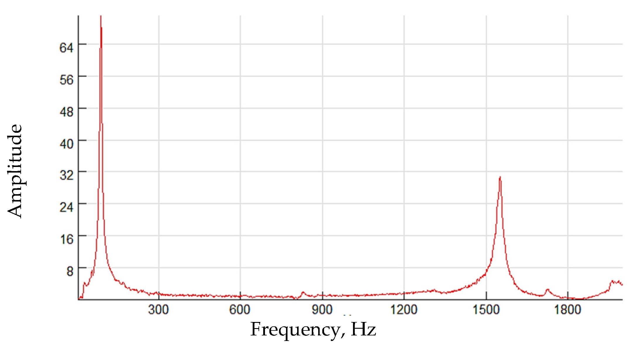
After removing the constant offset from F1 and F2, the signals are concatenated in the new signal and normalised. Based on the spectrum analysis (Figure 7), which represents the amplitude of the signal at each frequency component, the region of second pronounced peak is selected for further analysis. Infinite Impulse Response (IIR) filter with band-pass from 1200 Hz to 1800 Hz is used. The amplitude units on the y-axis of the spectrum are dependent on the units of the original signal recorded by the ADC device. As the original signal was recorded in arbitrary units, then the amplitude units of the spectrum are also in arbitrary units.

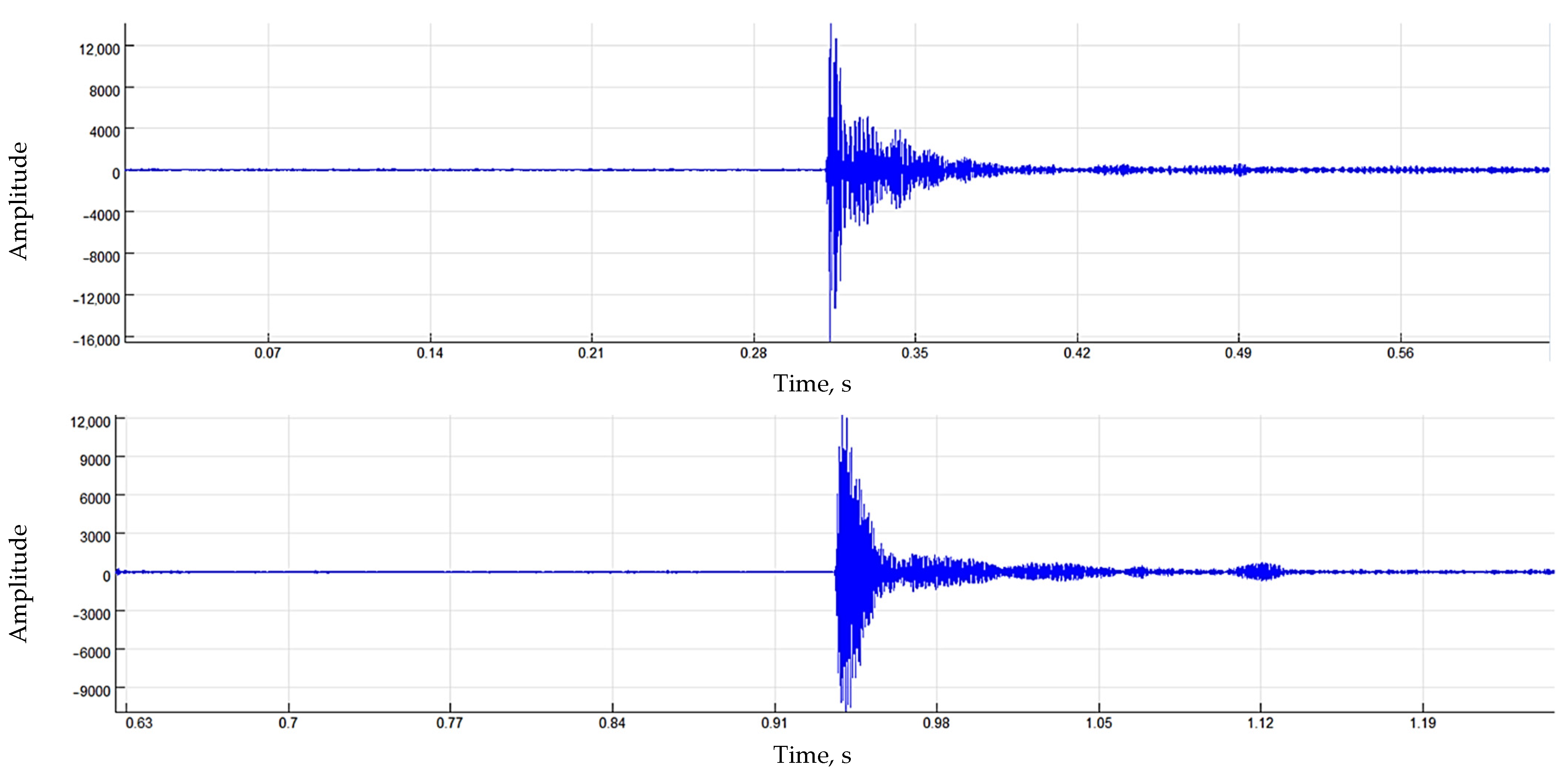
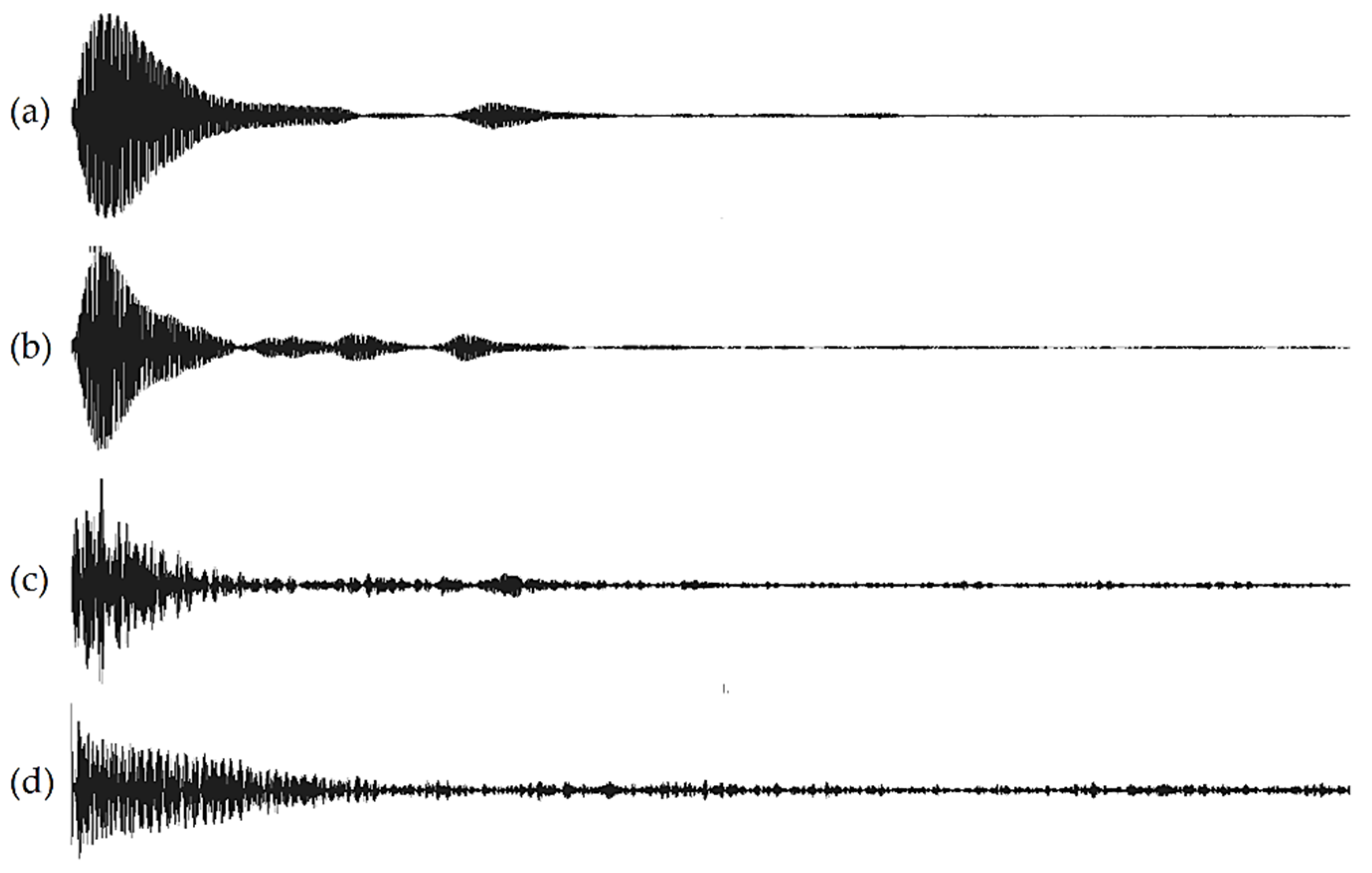
The split signals F1* and F2* after the IIR filter are shown in Figure 8.

Obtained product of convolution in the X-axis direction, which combines the pair of signals from both sensors and characterises the degree of similarity between two signals for four grades of joint stiffness, is shown in Figure 9.

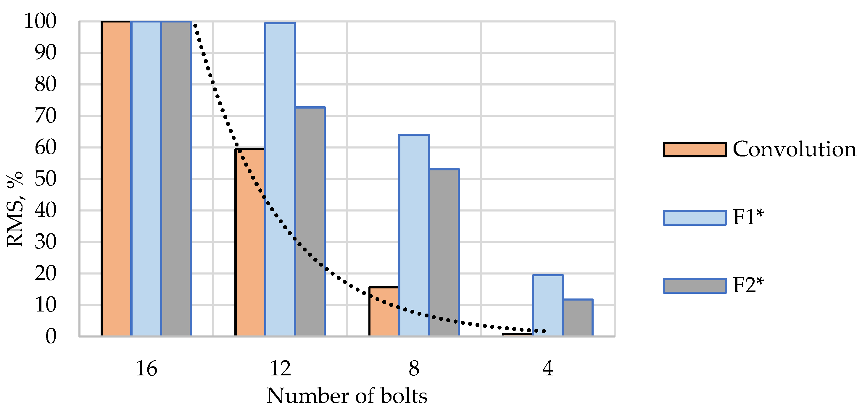
As can be seen from Figure 9, as the degree of joint degradation develops, its convolution shape changes. The representation of the convolutional signal becomes noisier as the joint degrades. As a convolution is integral that expresses the amount of overlap of one signal as it is shifted over another signal, it can be argued that as the joint degrades, the similarity of response signals from coaxially placed sensors on each side of the joint decreases. Quantitatively, this change can be expressed by the RMS of the convolution signal. RMS values of signals F1* and F2* and their convolution as a percentage from the corresponding maximal value are summarised in Figure 10.

It can be seen from Figure 10 that the RMS of sensors’ signals cannot provide a sufficient description of the joint stiffness grade. In the case of sensor 1, the difference between RMS for the joint with 16 bolts and 12 bolts is equal only to 0.6%. In the case of convolution of two coaxially collected signals, the RMS of convolution clearly shows a direct correlation between the calculated RMS value and the stiffness grades of the steel beam splice joint. The sensitivity of this parameter to changes in stiffness is high enough to be safe for a joint stiffness evaluation. These findings suggest that the coaxial correlation method with RMS of convolution signal can be used as indicators of joint stiffness in steel beam splice connections, providing valuable insights into the behaviour of these connections.

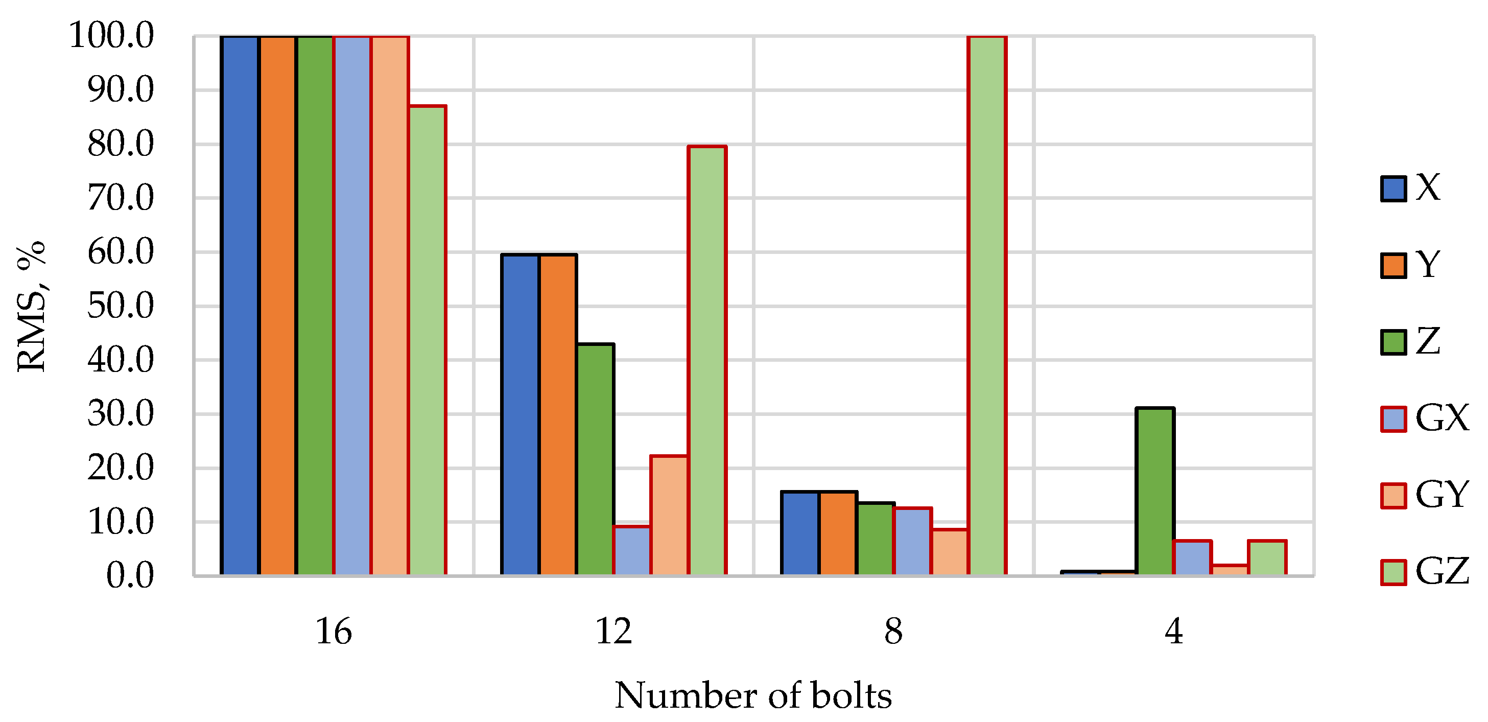
Figure 11 summarises the RMS values of convolution signals in 6D space. For the investigated type of splice joint, the RMS of convolution shows a direct correlation between the calculated RMS value and the stiffness grades of the joint in the X, Y and GY axes directions. In the GX axis, the obtained difference in RMS value for joints with 12, 8 and 4 bolts are not so pronounced for convenient and certain evaluation of joint stiffness. In the Z-axis direction, the increased RMS value was reached at a higher degree of joint degradation when the bottom metal plate was removed, and only the top 4 bolts were left. In the GZ axis, direction obtained data is not informative.

So, it can be concluded that the nature of the RMS during the degradation of the joint may change in different axes. If, in the case of simple joints, it is possible to predict which axes are better to investigate, then in the case of complex joints, wrongly chosen axes may lead to wrong conclusions regarding the state of the investigated joint. Therefore, the relationships obtained with the simple splice joint considered in this work confirm the usefulness of 6D measurements and increase the reliability of the interpretation of quality assessment of structural joints.

4. Conclusions

The novel method of coaxial correlation in 6D space for quality assessment of moment-resisting structural joints, including a system response analysis method with coaxially placed 6D sensors on either side of the joint and electronic system, is proposed. The improvements of the initial version of the coaxial correlation method provide the possibilities of:

• Determining linear accelerations and angular velocities, thus providing a measurement option in 6D space;
• Analysing at frequencies higher than 500 Hz, which is essential to ensure the possibility of studying the prototype of the structural joint in laboratory conditions;
• Processing data in the time domain thanks to synchronisation between the input signal and system responses;
• Using even weak input signal thanks to averaging system response.

The developed approach of collected data post-processing using convolution signals from both sensors makes it possible to estimate damage or degradation of the structural joint during its operation both visually by changes in the appearance of the convolution signal and also quantitatively by the suggested RMS value. Measurements in 6D space provide the reliability of the result interpretation. Mostly direct correlation between the calculated RMS values of convolution signals and the stiffness grades of the structural joint is obtained during the verification of the proposed method. It means that as the stiffness of the moment-resisting structural joint decreases, the similarity of the response signals from both sides of the joint also decreases. The results obtained from testing the proposed method on a simple model with a bolted joint demonstrate that the method can be effectively used to assess the quality of moment-resisting joints. Moreover, this method shows promise as a solution for assessing more complex joints, as well as welded joints.