
Simplified Procedure for Rapidly Estimating Inelastic Responses of Numerous High-Rise Buildings with Reinforced Concrete Shear Walls
Abstract
:1. Introduction
2. UMRHA Procedure
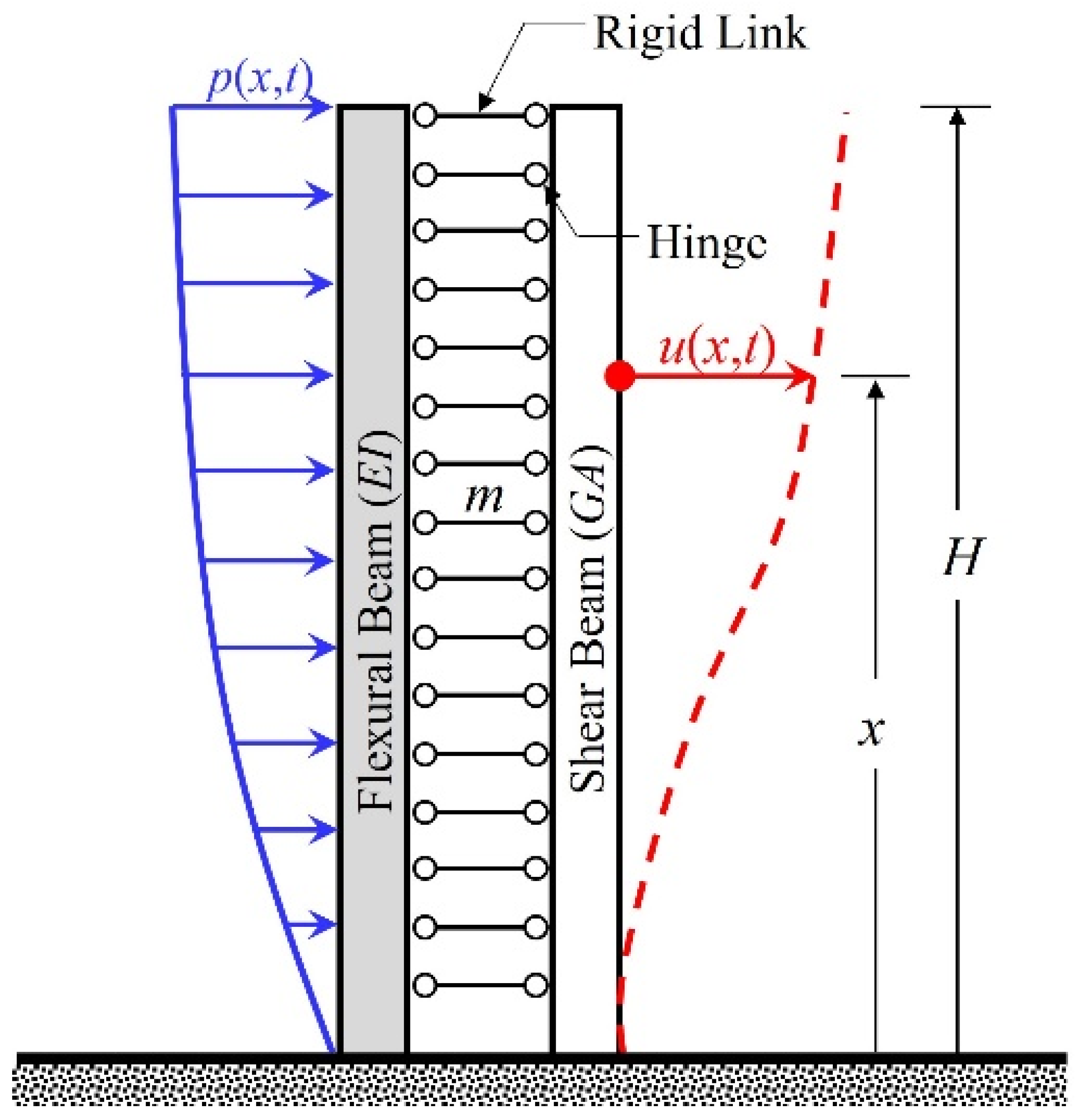
3. CSFCBM
4. Case Study Buildings
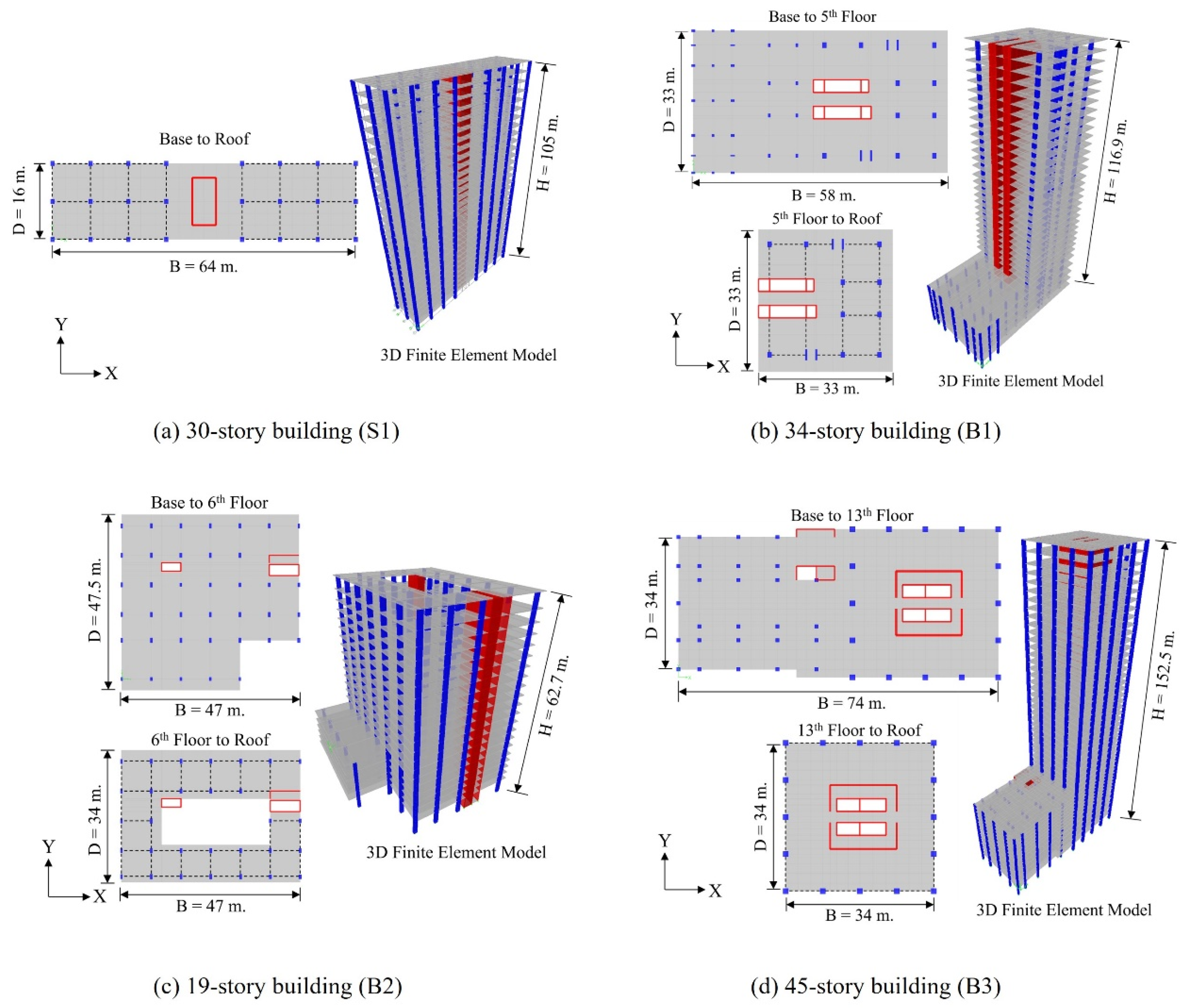
4.1. FEM of Case Study Building
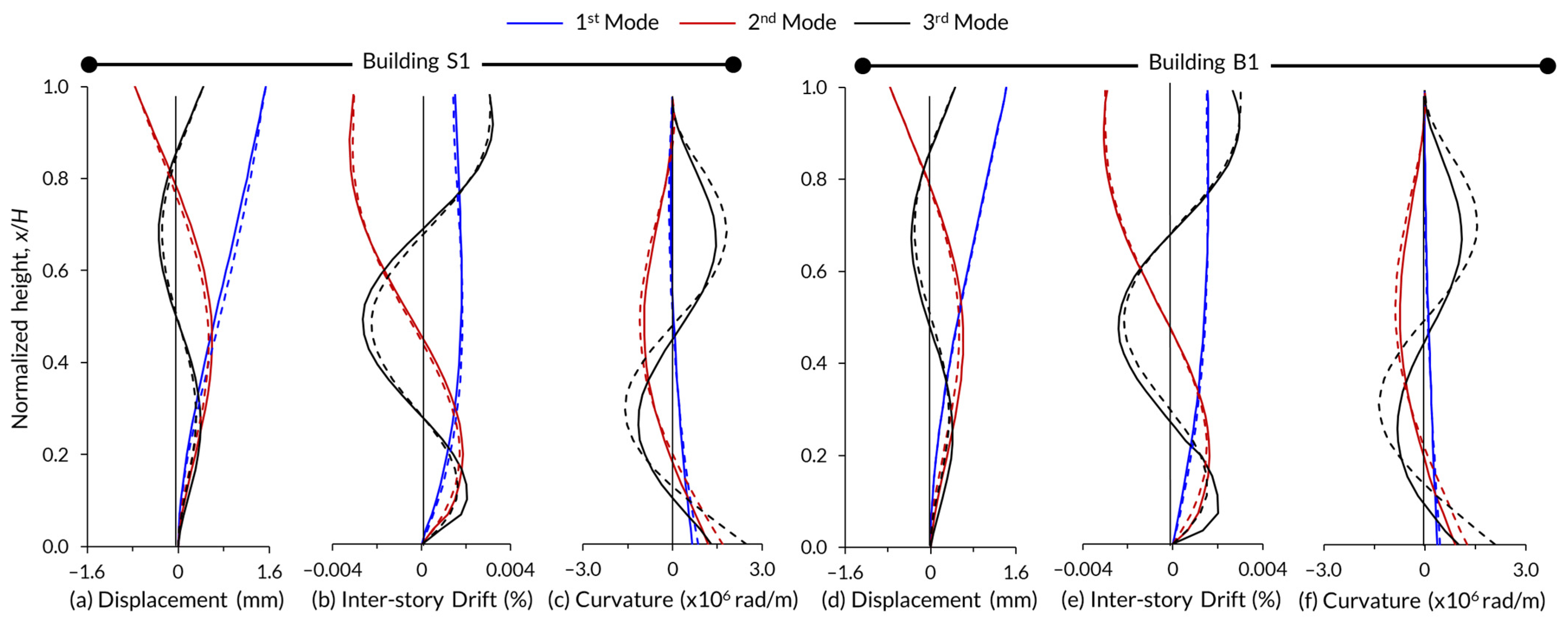
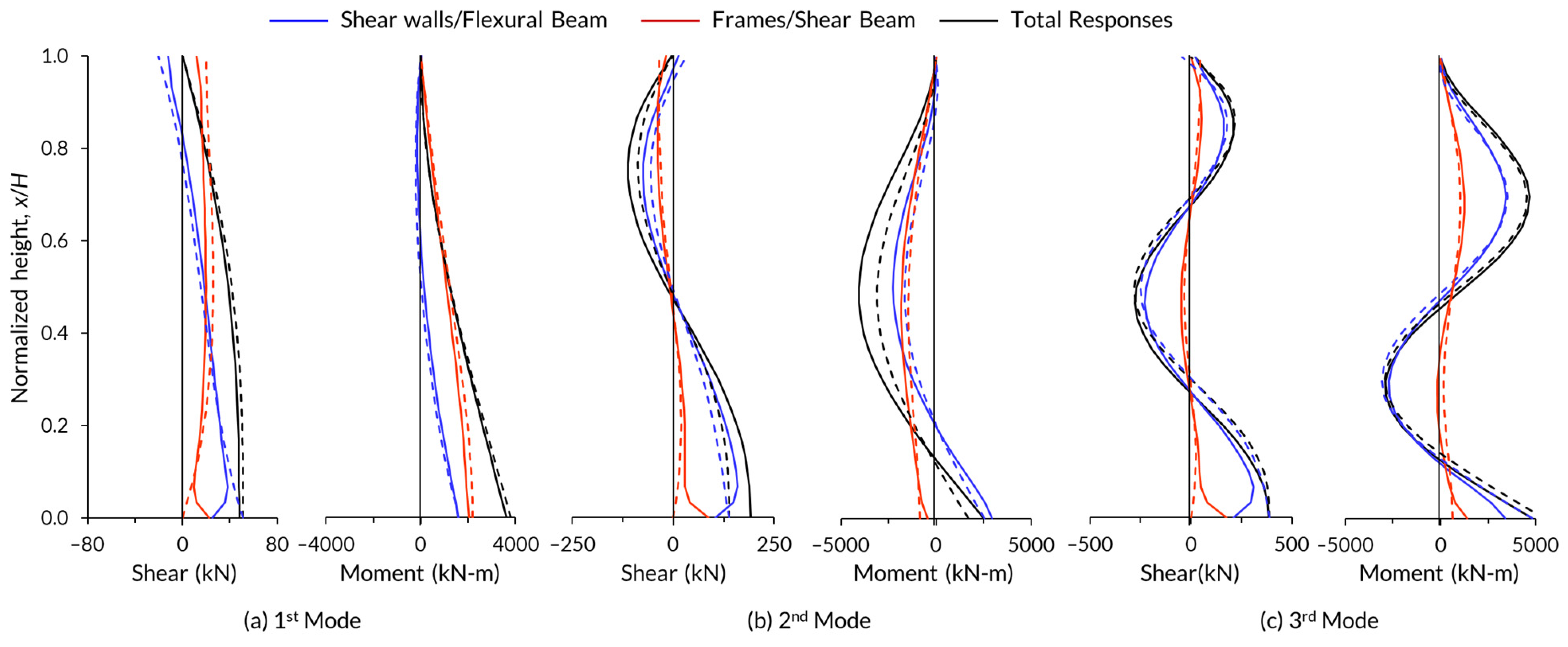
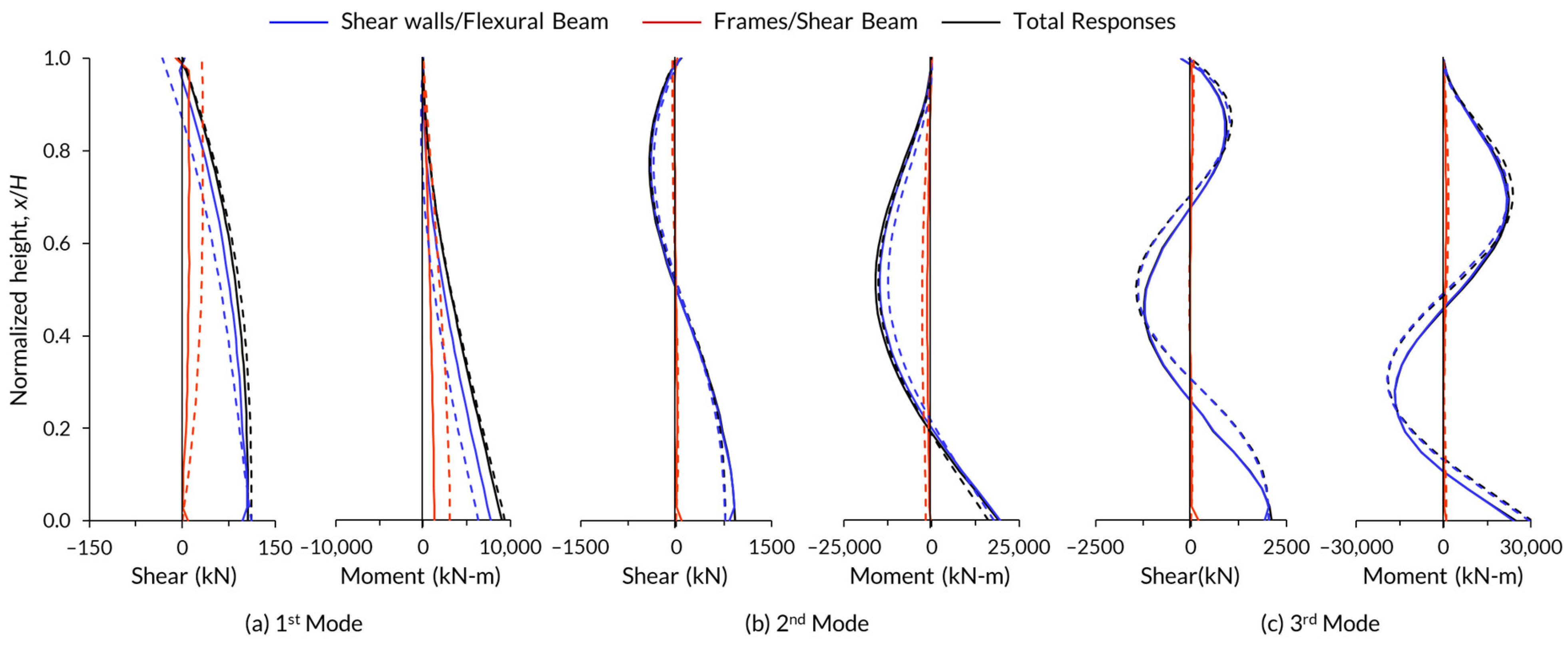
4.2. Accuracy of CSFCBM in Estimating the Modal Properties and Responses
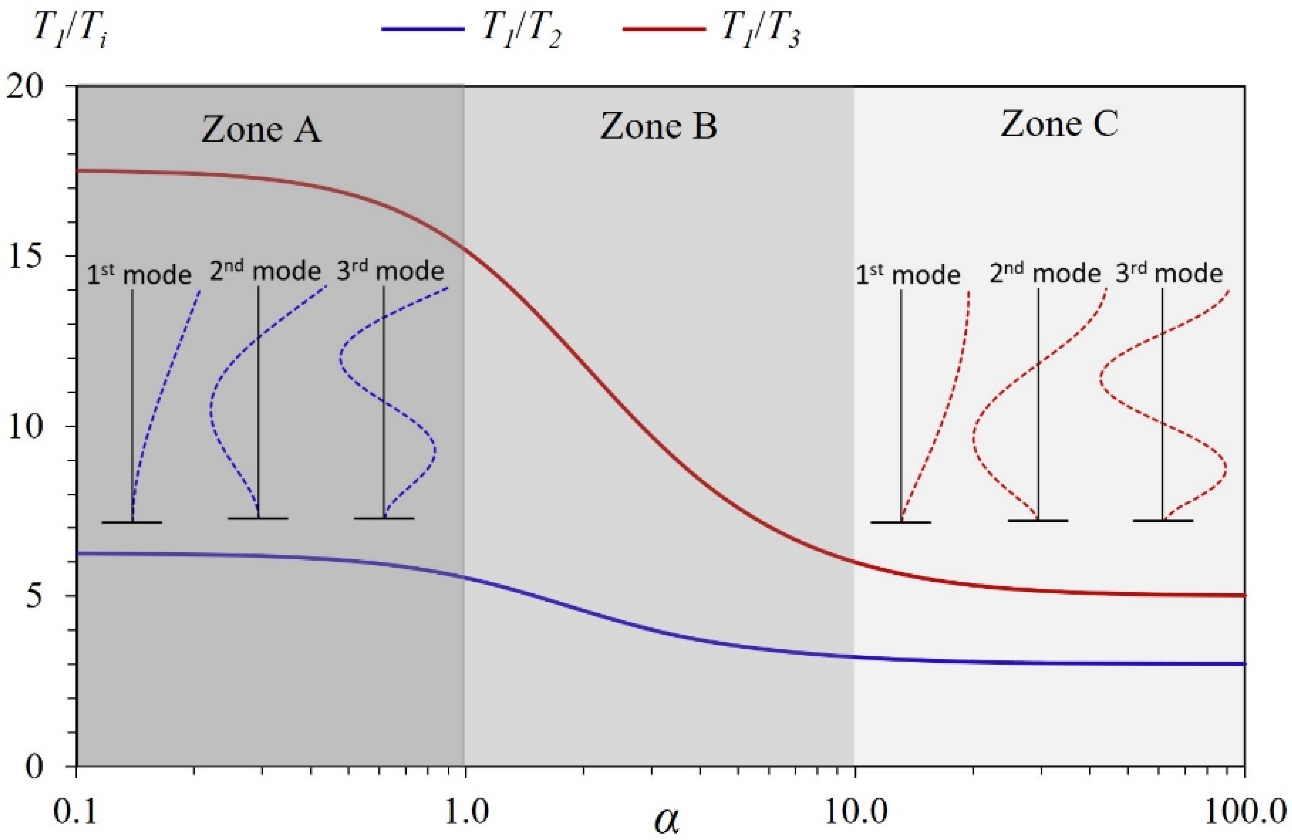
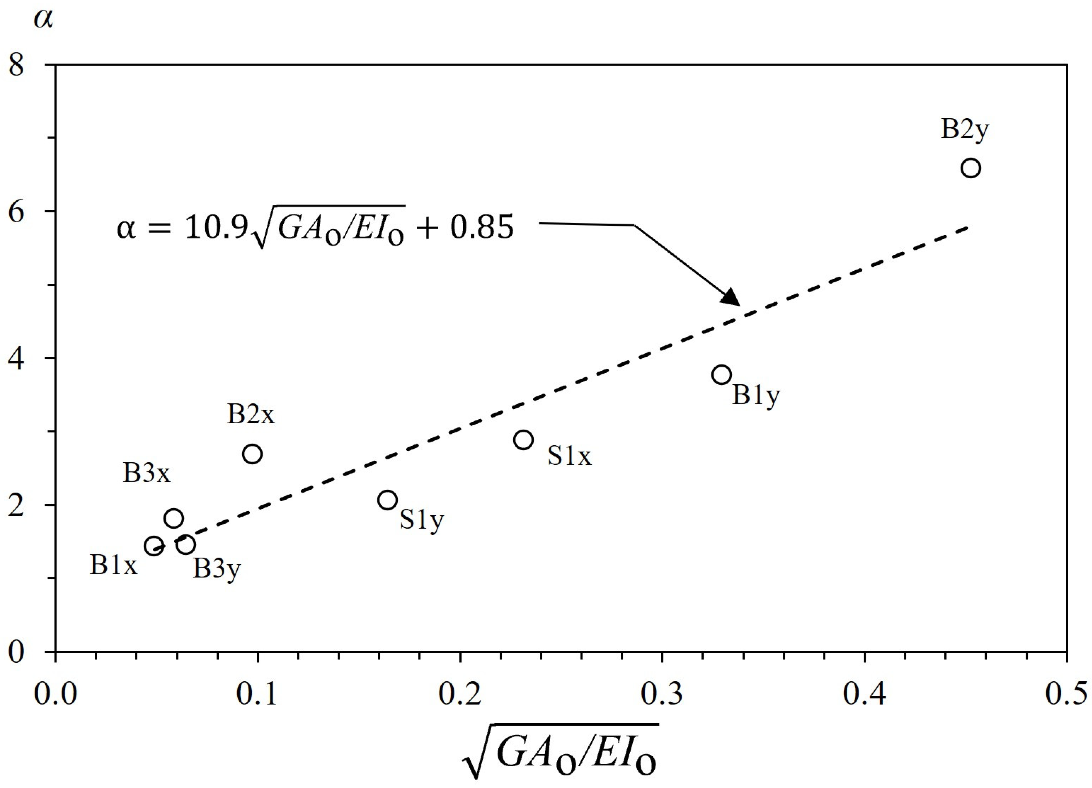
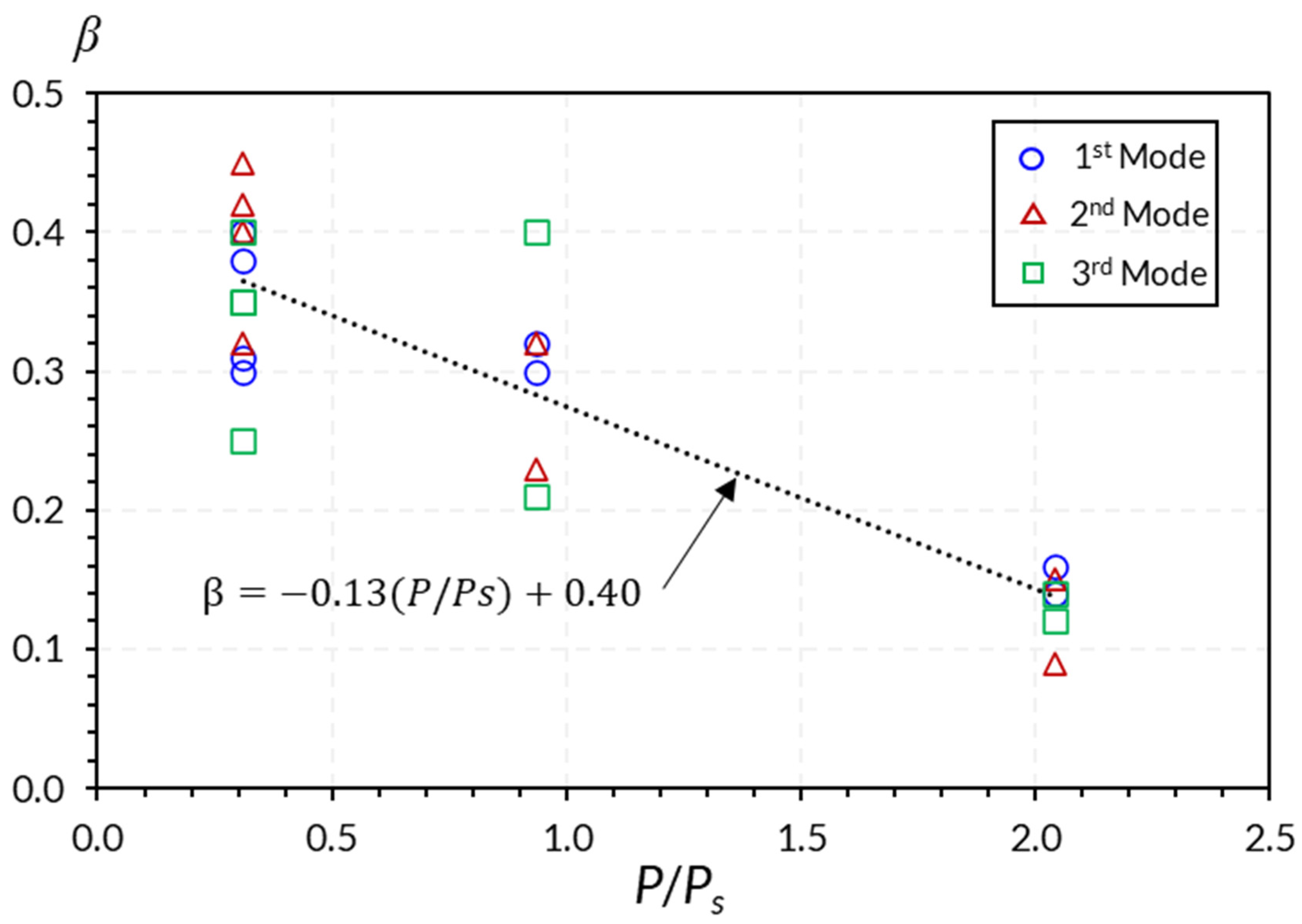
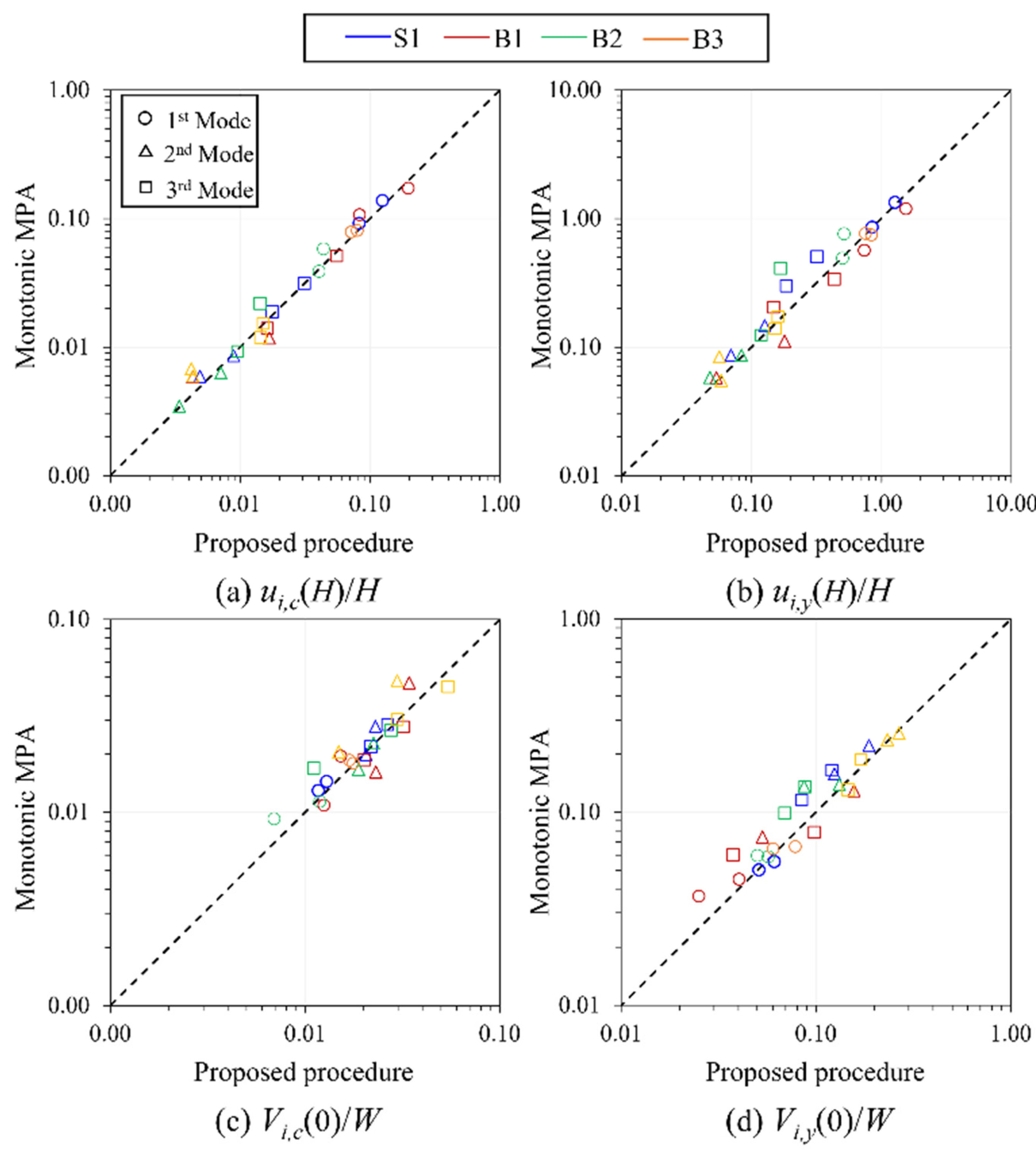
4.3. Estimation of α-Value
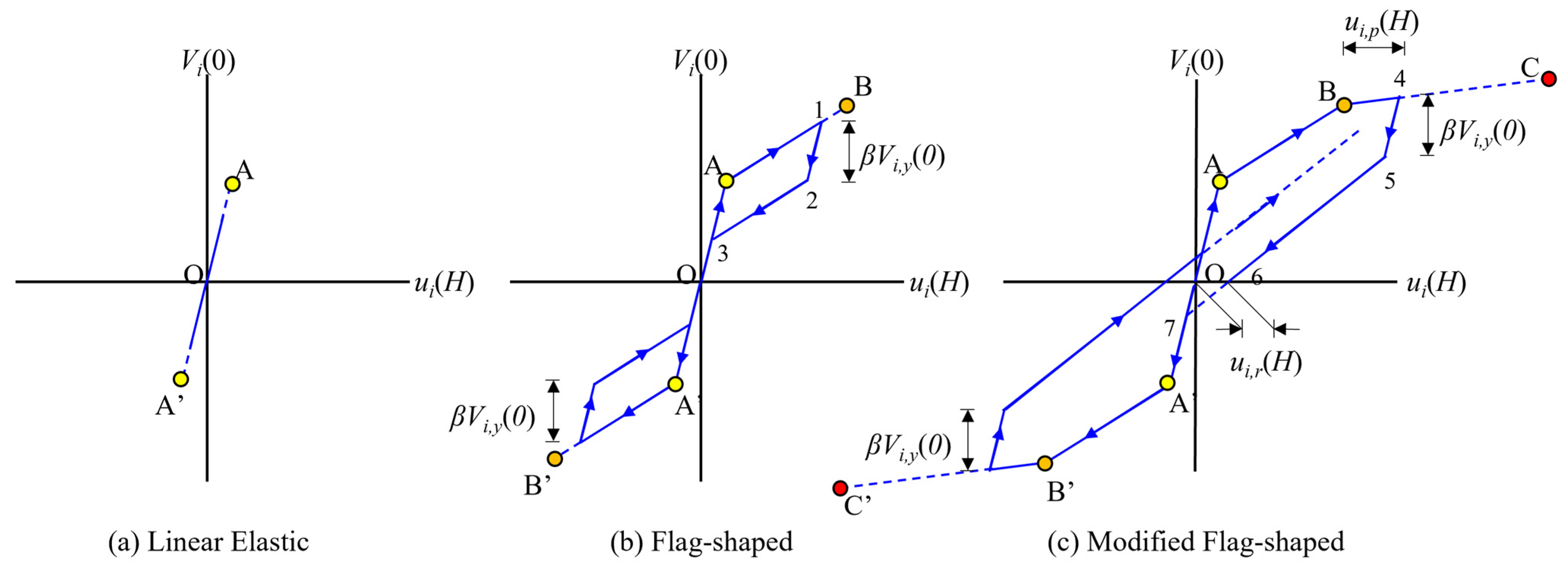
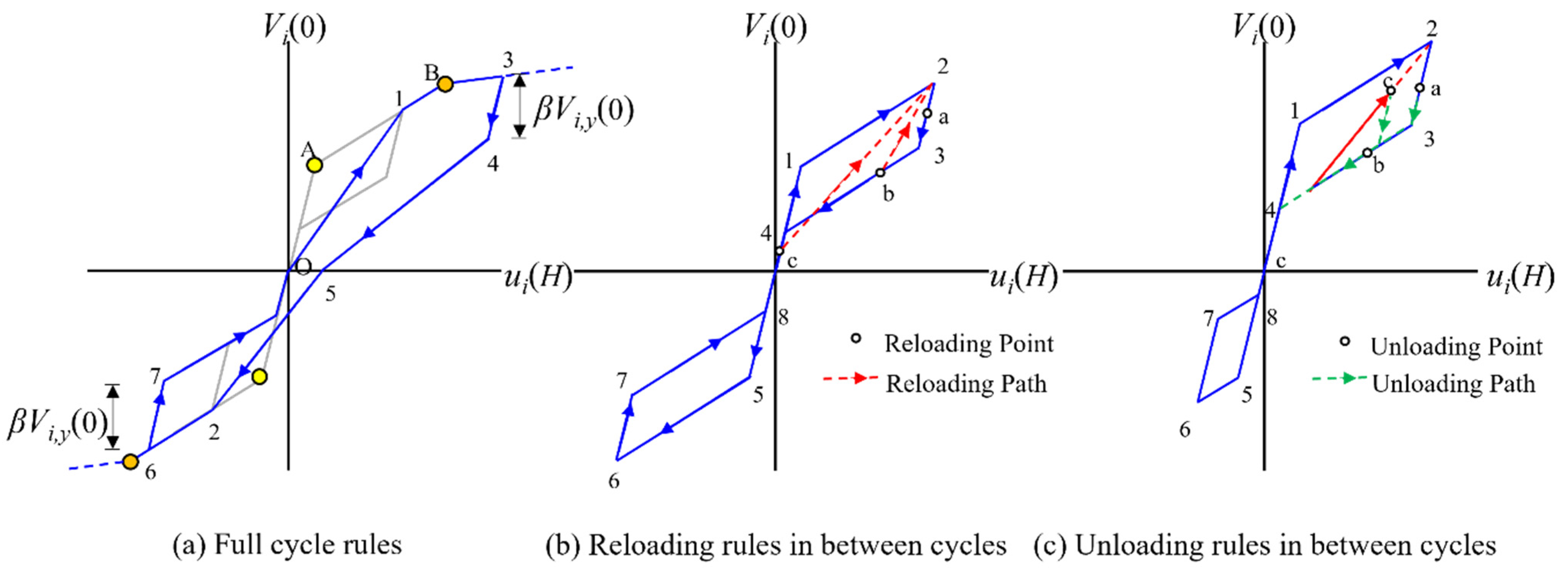
5. Modal Hysteretic Model
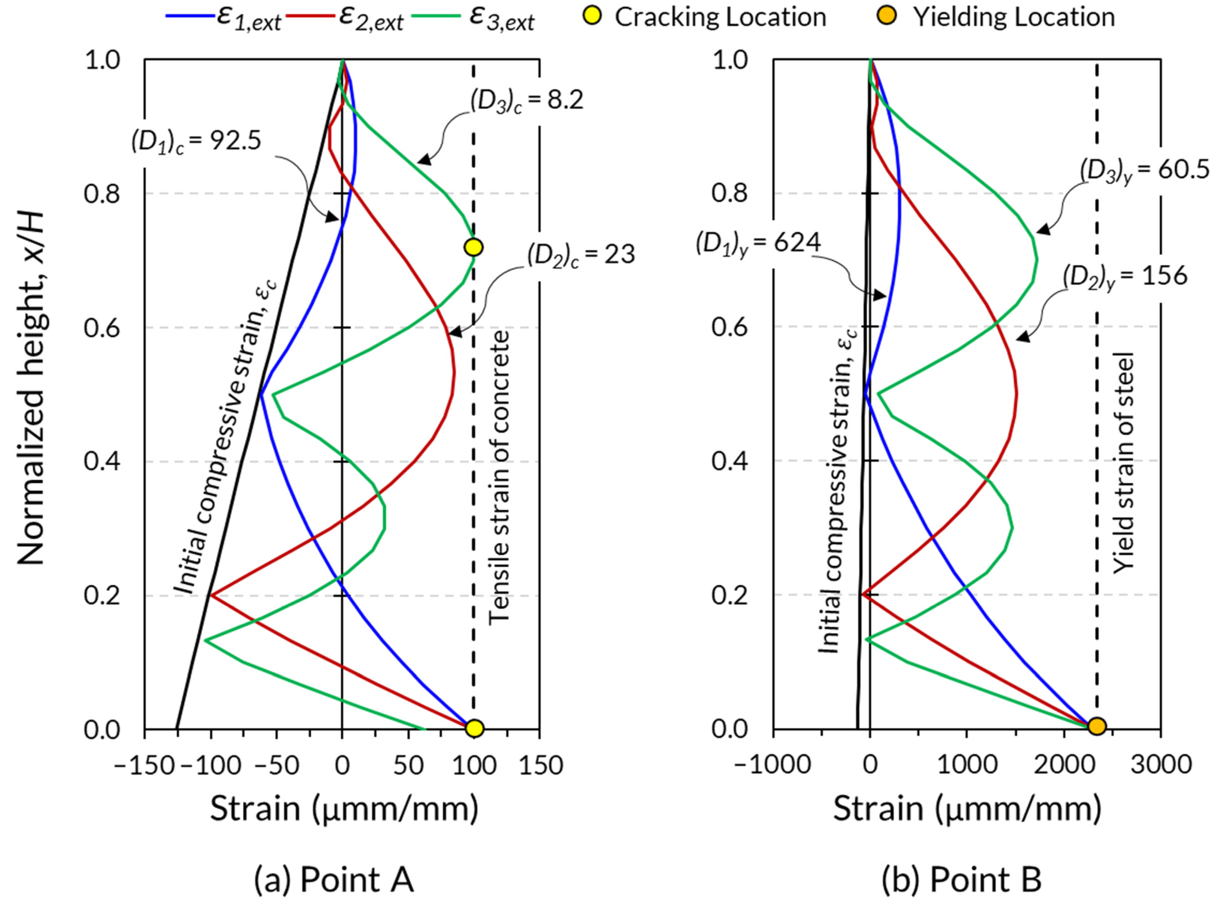
5.1. Modal Hysteretic Behavior
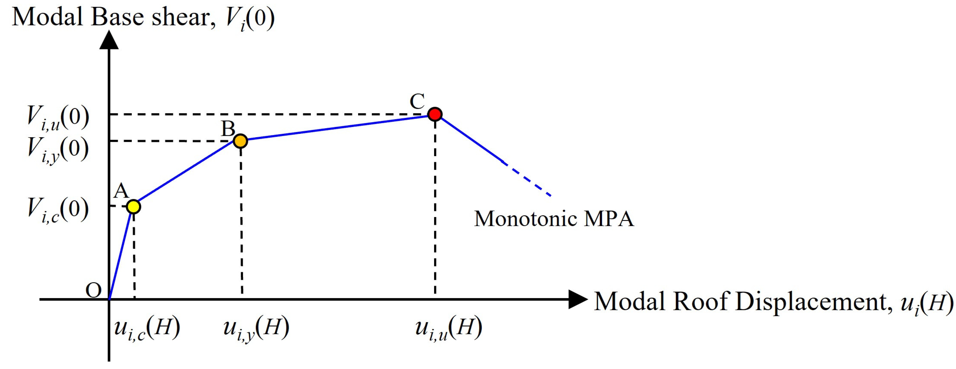
5.2. Construction of the Modal Hysteretic Model Using CSFCBM
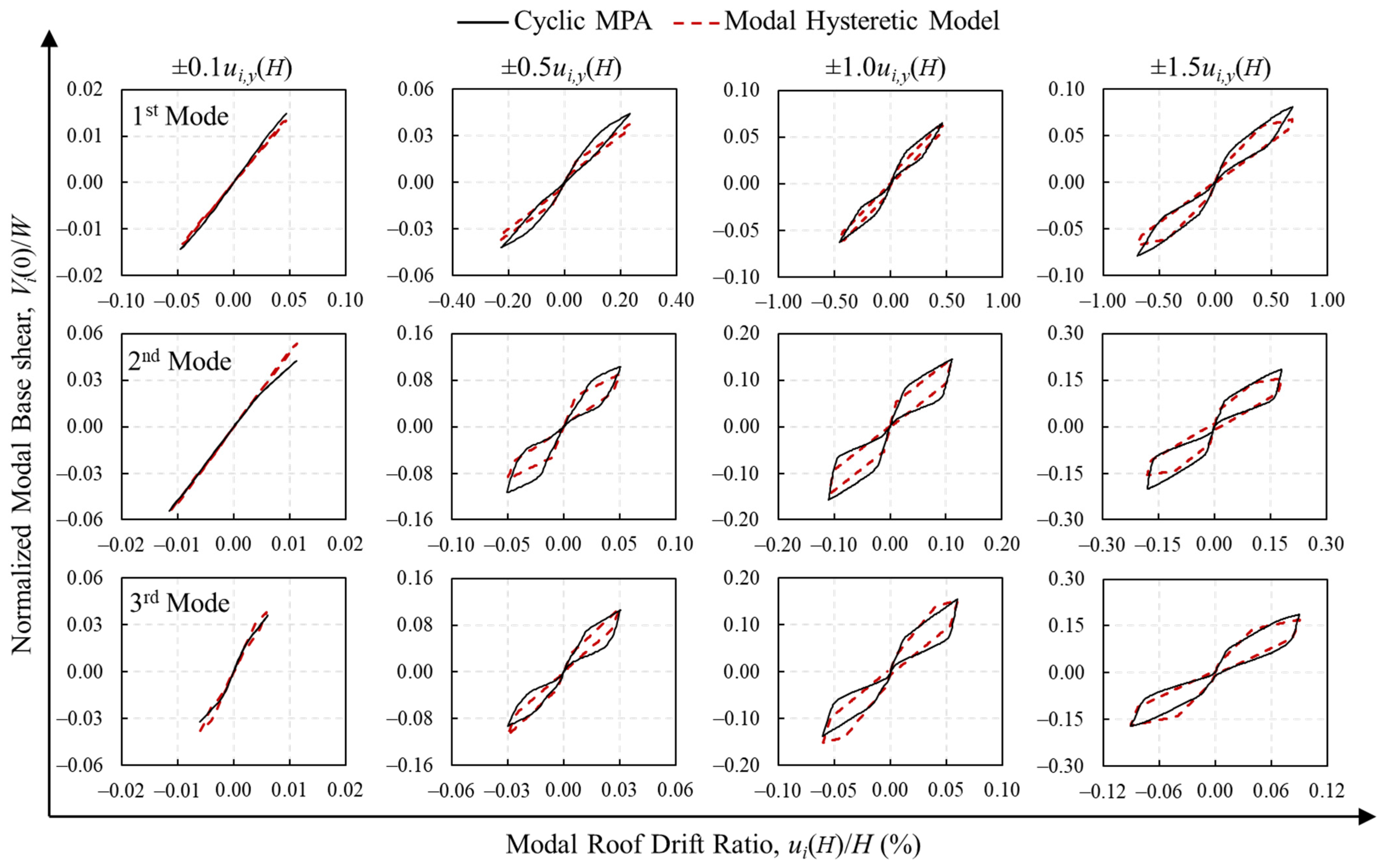
5.3. Verification of the Modal Hysteretic Model
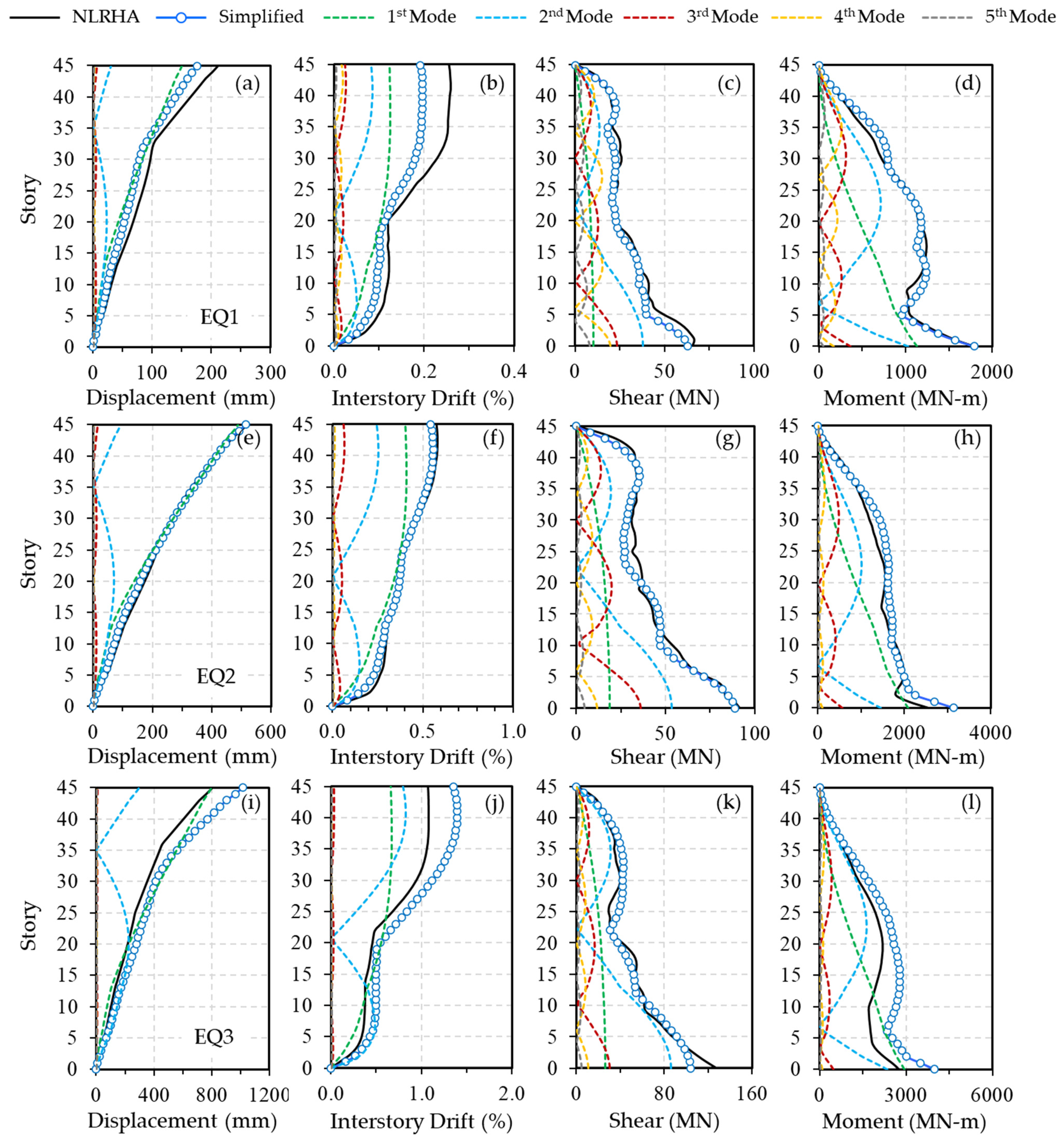
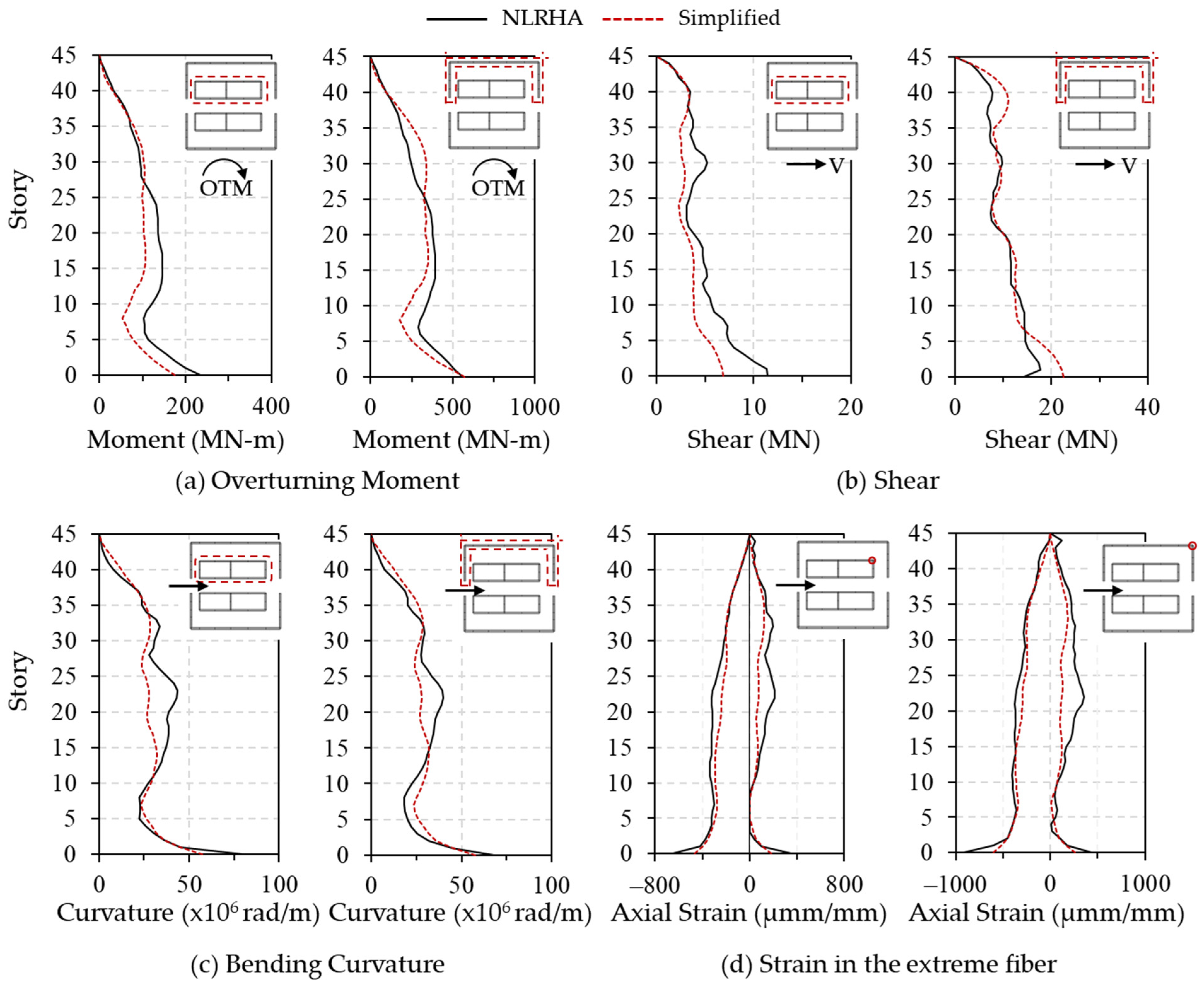
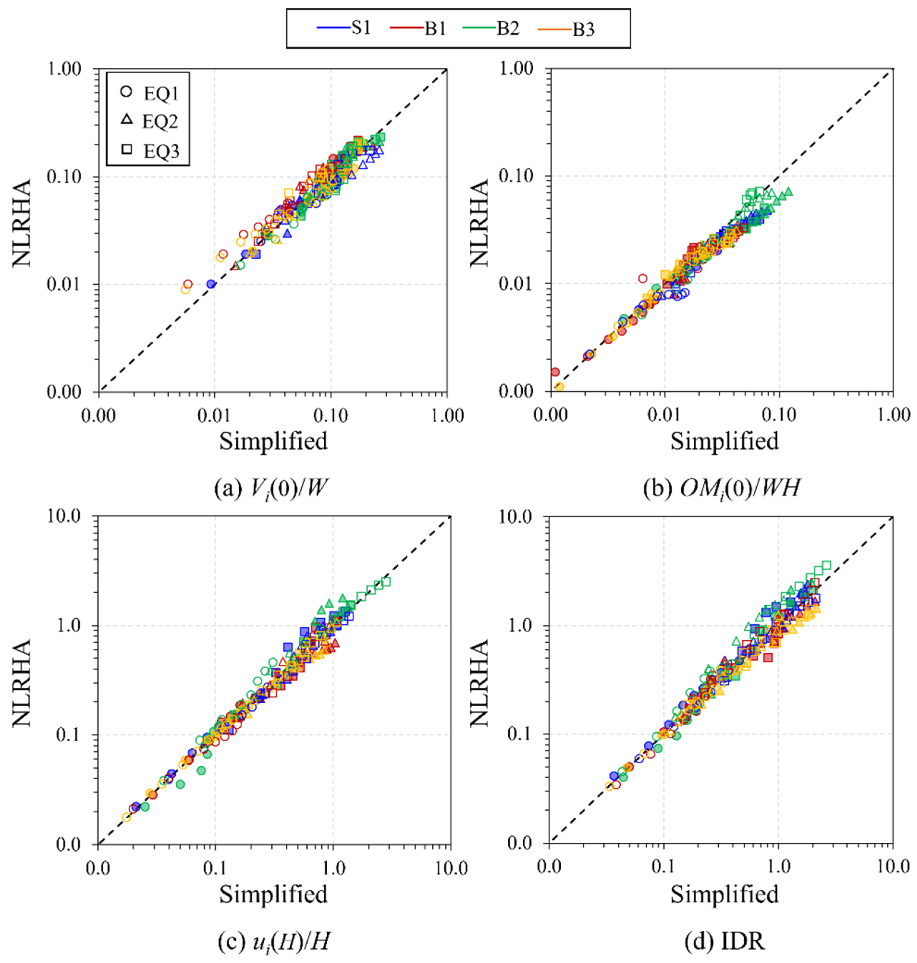
6. Verification of the Simplified Procedure
7. Conclusions
Supplementary Materials
Author Contributions
Funding
Data Availability Statement
Conflicts of Interest
References
- Maffei, J.; Yuen, N. Seismic performance and design requirements for high-rise buildings. Struct. Mag. 2007, 28–32. Available online: https://www.structuremag.org/wp-content/uploads/2014/09/F-HighRise-Maffei-Apr07-online-version1.pdf (accessed on 8 December 2021).
- Kayvani, K. Design of high-rise buildings: Past, present and future. In Proceedings of the 23rd Australasian Conference on the Mechanics of Structures and materials (ACMSM23), Byron Bay, Australia, 9–12 December 2014; pp. 15–20. [Google Scholar]
- Guidelines Working Group. TBI: Guidelines for Performance-Based Seismic Design of Tall Buildings; PEER Report No. 2010/05; University of California: Berkeley, CA, USA, 2010. [Google Scholar]
- Su, R.K.L.; Chandler, A.M.; Sheikh, M.N.; Lam, N.T.K. Influence of non-structural components on lateral stiffness of tall buildings. Struct. Des. Tall Spec. Build. 2005, 14, 143–164. [Google Scholar] [CrossRef] [Green Version]
- Kreslin, M.; Fajfar, P. The extended N2 method taking into account higher mode effects in elevation. Earthq. Eng. Struct. Dyn. 2011, 40, 1571–1589. [Google Scholar] [CrossRef]
- Pekelnicky, R.; Engineers, S.D.; Chris Poland, S.E.; Engineers, N.D. ASCE 41-13: Seismic evaluation and retrofit rehabilitation of existing buildings. In Proceedings of the SEAOC-SEANM Convention, Santa Fe, NM, USA, 12–15 September 2012. [Google Scholar]
- American Society of Civil Engineers. Minimum Design Loads and Associated Criteria for Buildings and Other Structures; American Society of Civil Engineers: Reston, VA, USA, 2017. [Google Scholar]
- Remo, J.W.; Pinter, N. Hazus-MH earthquake modeling in the central USA. Nat. Hazards 2012, 63, 1055–1081. [Google Scholar] [CrossRef]
- Chopra, A.K.; Goel, R.K. A Modal Pushover Analysis Procedure to Estimate Seismic Demands for Buildings: Theory and Preliminary Evaluation; Pacific Earthquake Engineering Research (PEER) Centre: Berkeley, CA, USA, 2001. [Google Scholar]
- Chopra, A.K.; Goel, R.K. A modal pushover analysis procedure for estimating seismic demands for buildings. Earthq. Eng. Struct. Dyn. 2002, 31, 561–582. [Google Scholar] [CrossRef] [Green Version]
- Miranda, E.; Akkar, S.D. Generalized interstory drift spectrum. J. Struct. Eng. 2006, 132, 840–852. [Google Scholar] [CrossRef] [Green Version]
- Munir, A.; Warnitchai, P. The cause of unproportionately large higher mode contributions in the inelastic seismic responses of high-rise core-wall buildings. Earthq. Eng. Struct. Dyn. 2012, 41, 2195–2214. [Google Scholar] [CrossRef]
- Mehmood, T.; Warnitchai, P.; Suwansaya, P. Seismic evaluation of tall buildings using a simplified but accurate analysis procedure. J. Earthq. Eng. 2018, 22, 356–381. [Google Scholar] [CrossRef]
- Najam, F.A.; Warnitchai, P. A modified response spectrum analysis procedure to determine nonlinear seismic demands of high-rise buildings with shear walls. Struct. Des. Tall Spec. Build. 2018, 27, e1409. [Google Scholar] [CrossRef]
- Khan, F.R.; Sbarounis, J.A. Interaction of shear walls and frames. J. Struct. Div. 1964, 90, 285–335. [Google Scholar] [CrossRef]
- Heidebrecht, A.C. Approximate analysis of tall wall-frame structures, B.S. Smith. J. Struct. Div. 1973, 99, 199–221. [Google Scholar] [CrossRef]
- Smith, B.S.; Kuster, M.; Hoenderkamp, J.C.D. A generalized approach to the deflection analysis of braced frame, rigid frame, and coupled wall structures. Can. J. Civ. Eng. 1981, 8, 230–240. [Google Scholar] [CrossRef]
- Smith, B.S.; Kuster, M.; Hoenderkamp, J.C.D. Generalized method for estimating drift in high-rise structures. J. Struct. Eng. 1984, 110, 1549–1562. [Google Scholar] [CrossRef]
- Nollet, M.J.; Smith, B.S. Behavior of curtailed wall-frame structures. J. Struct. Eng. 1993, 119, 2835–2854. [Google Scholar] [CrossRef]
- Miranda, E. Approximate seismic lateral deformation demands in multistory buildings. J. Struct. Eng. 1999, 125, 417–425. [Google Scholar] [CrossRef]
- Miranda, E.; Reyes, C.J. Approximate lateral drift demands in multistory buildings with nonuniform stiffness. J. Struct. Eng. 2002, 128, 840–849. [Google Scholar] [CrossRef]
- Miranda, E.; Taghavi, S. Approximate floor acceleration demands in multistory buildings. J. Struct. Eng. 2005, 131, 203–211. [Google Scholar] [CrossRef]
- Reinoso, E.; Miranda, E. Estimation of floor acceleration demands in high-rise buildings during earthquakes. Struct. Des. Tall Spec. Build. 2005, 14, 107–130. [Google Scholar] [CrossRef]
- Khaloo, A.R.; Khosravi, H. Multi-mode response of shear and flexural buildings to pulse-type ground motions in near-field earthquakes. J. Earthq. Eng. 2008, 12, 616–630. [Google Scholar] [CrossRef]
- Xiong, H.; Zheng, Y.; Chen, J. A nonlinear computational model for regional seismic simulation of tall buildings. Int. J. High-rise Build. 2020, 9, 273–282. [Google Scholar] [CrossRef]
- Kittiwuthikum, K. Effects of Foundation Flexibility on Dynamic Properties of Buildings in Bangkok. Ph.D. Thesis, Asian Institute of Technology, Khlong Nueng, Thailand, 2004. Available online: http://203.159.12.58/ait-thesis/detail.php?id=B08991 (accessed on 8 December 2021).
- Singlumpong, T. Effects of Pile Foundation Flexibility on the Dynamic Characteristics of Multi-Story Buildings in Bangkok. Ph.D. Thesis, Asian Institute of Technology, Khlong Nueng, Thailand, 2006. Available online: http://203.159.12.58/ait-thesis/detail.php?id=B10088 (accessed on 8 December 2021).
- Perform3D. Nonlinear Analysis and Performance Assessment for 3D Structures Version 7; Computers and Structures, Inc. (CSI): Berkeley, CA, USA, 2018. [Google Scholar]
- Orakcal, K.; Wallace, J.W. Flexural modeling of reinforced concrete walls-model attributes, J.P. Conte. Struct. J. 2004, 101, 688–698. [Google Scholar]
- Wallace, J.W. Behavior, design, and modeling of structural walls and coupling beams. Lessons from recent laboratory tests and earthquakes. Int. J. Concr. Struct. Mater. 2012, 6, 3–18. [Google Scholar] [CrossRef] [Green Version]
- LATSBC. The Structural Design of Tall and Special Buildings; John Wiley & Sons Ltd.: Hoboken, NJ, USA, 2017. [Google Scholar]
- Mander, J.B.; Priestley, M.J.N.; Park, R. Theoretical stress–strain model for confined concrete. J. Struct. Eng. 1988, 114, 1804–1826, 1827–1849. [Google Scholar] [CrossRef] [Green Version]
- ACI Committee 318. Building Code Requirements for Structural Concrete (ACI318M-11) and Commentary; American Concrete Institute: Farmington Hills, MI, USA, 2011. [Google Scholar]
- Paulay, T.; Priestley, M.J.N. Seismic Design of Reinforced Concrete and Masonry Buildings; John Wiley & Sons: Hoboken, NJ, USA, 1992. [Google Scholar]
- Kappos, A.J.; Stylianidis, K.C.; Michailidis, C.N. Analytical models for brick masonry infilled R/C frames under lateral loading. J. Earthq. Eng. 1998, 2, 59–87. [Google Scholar] [CrossRef]
- ACI Code-530.1-11/ ASCE 6-11; Building Code Requirements and Specifications for Masonry; Masonry Standards Joint Committee (MSJC): Boulder, CO, USA, 2011; pp. 602–611.
- Suwansaya, P. Simplified Analysis Procedure to Determine the Nonlinear Seismic Demands of High-Rise Building with Reinforced Concrete Shear Walls. Ph.D. Thesis, Asian Institute of Technology (AIT), Khlong Nueng, Thailand, 2023. [Google Scholar]
- Pandey, S.; Warnitchai, P.; Vasanthapragash, N.; Najam, F. Development of modal hysteretic model for the seismic response analysis of tall buildings with RC shear wall. In Proceedings of the 7th Asia Conference on Earthquake Engineering, Bangkok, Thailand, 22–25 November 2018. [Google Scholar]
- Pandey, S. Development of Modal Hysteretic Model for the Seismic Response Analysis of Tall Buildings with RC Shear Wall. Master’s Thesis, Department of Civil and Infrastructure Engineering. Asian Institute of Technology, Pathum Thani, Thailand, 2017. [Google Scholar]
- McKenna, F. OpenSees: A framework for earthquake engineering simulation. Comput. Sci. Eng. 2011, 13, 58–66. [Google Scholar] [CrossRef]
- Ancheta, T.D.; Darragh, R.B.; Stewart, J.P.; Seyhan, E.; Silva, W.J.; Chiou, B.S.; Wooddell, K.E.; Graves, R.W.; Kottke, A.R.; Boore, D.M.; et al. NGA-West2 database. Earthq. Spectra 2014, 30, 989–1005. [Google Scholar] [CrossRef]


| Building Name | S1 | B1 | B2 | B3 | |
|---|---|---|---|---|---|
| Width of the tower, B (m) | 64.0 | 31.0 | 47.0 | 33.6 | |
| Depth of the tower, D (m) | 16.0 | 32.5 | 34.0 | 33.6 | |
| Height, H (m) | 105.0 | 116.9 | 59.5 | 152.5 | |
| No. of stories | 30 | 34 | 19 | 45 | |
| Typical story height, h (m) | 3.5 | 3.2 | 2.9 | 3.5 | |
| RC wall section area/footprint area (%) | 0.88 | 1.62 | 0.54 | 2.42 | |
| RC column section area/footprint area (%) | 2.81 | 1.45 | 1.06 | 2.04 | |
| RC typical wall thickness (m) | Base–10th floor | 0.35 | 0.25 | 0.25 | 0.45 |
| 10th–20th floor | 0.35 | 0.25 | 0.25 | 0.40 | |
| 20th floor–roof | 0.35 | 0.25 | 0.25 | 0.35 | |
| RC column typical dimension (m) | Base–10th floor | 1.0 × 1.2 | 0.9 × 1.2 | 0.5 × 1.2 | 1.2 × 1.2 |
| 10th–20th floor | 1.0 × 1.2 | 0.9 × 1.2 | 0.5 × 1.2 | 1.2 × 1.2 | |
| 20th floor–roof | 1.0 × 1.2 | 0.9 × 1.2 | 0.5 × 1.2 | 1.2 × 1.2 | |
| Longitudinal reinforcement ratio in RC wall (%) | Base–10th floor | 4.0 | 1.27 | 2.27 | 2.95 |
| 10th–20th floor | 4.0 | 0.81 | 1.45 | 1.44 | |
| 20th floor–roof | 4.0 | 0.46 | 0.93 | 1.44 | |
| Specified compressive strength of concrete, (MPa) | RC walls | 45 | 45 | 42 | 45 |
| RC column | 45 | 32 | 42 | 40 | |
| RC and PT slabs * | 32 | 32 | 32 | 32 | |
| Specified yield strength of longitudinal reinforcement steel bar, fy (MPa) | 490 | 390 | 390 | 390 | |
| Modal Properties | X Direction | Y Direction | |||||
|---|---|---|---|---|---|---|---|
| FEM | CSFCBM | Error (%) | FEM | CSFCBM | Error (%) | ||
| Ti (s) | First mode | 4.420 | 4.420 | - | 3.371 | 3.371 | - |
| Second mode | 1.088 | 1.089 | - | 0.744 | 0.745 | - | |
| Third mode | 0.477 | 0.447 | 6.4 | 0.322 | 0.289 | 10.3 | |
| Mi/MT | First mode | 0.677 | 0.666 | 1.6 | 0.657 | 0.647 | 1.6 |
| Second mode | 0.162 | 0.143 | 11.8 | 0.184 | 0.159 | 13.5 | |
| Third mode | 0.063 | 0.059 | 6.0 | 0.065 | 0.062 | 5.1 | |
| Гi | First mode | 1.465 | 1.477 | 0.8 | 1.503 | 1.514 | 0.7 |
| Second mode | −0.724 | −0.767 | 6.1 | −0.757 | −0.810 | 7.0 | |
| Third mode | 0.414 | 0.495 | 19.5 | 0.411 | 0.502 | 22.0 | |
| T1/T2 | 4.063 | 4.531 | |||||
| A | 2.88 | 2.06 | |||||
| Modal Properties | X Direction | Y Direction | |||||
|---|---|---|---|---|---|---|---|
| FEM | CSFCBM | Error (%) | FEM | CSFCBM | Error (%) | ||
| Ti (s) | First mode | 3.112 | 3.112 | - | 5.487 | 5.487 | - |
| Second mode | 0.613 | 0.613 | - | 1.457 | 1.457 | - | |
| Third mode | 0.263 | 0.229 | 13.0 | 0.676 | 0.634 | 6.3 | |
| Mi/MT | First mode | 0.597 | 0.631 | 5.8 | 0.649 | 0.685 | 5.6 |
| Second mode | 0.200 | 0.172 | 14.0 | 0.135 | 0.129 | 4.6 | |
| Third mode | 0.085 | 0.063 | 25.6 | 0.059 | 0.056 | 4.7 | |
| Гi | First mode | 1.525 | 1.539 | 0.9 | 1.435 | 1.438 | 0.2 |
| Second mode | −0.814 | −0.838 | 3.0 | −0.689 | −0.721 | 4.6 | |
| Third mode | 0.490 | 0.506 | 3.2 | 0.429 | 0.485 | 13.0 | |
| T1/T2 | 5.077 | 3.766 | |||||
| A | 1.43 | 3.76 | |||||
| Building Name | X Direction | Y Direction | ||||||
|---|---|---|---|---|---|---|---|---|
| S1 | B1 | B2 | B3 | S1 | B1 | B2 | B3 | |
| Height of the building, H (m) | 105.0 | 116.9 | 59.5 | 152.5 | 105.0 | 116.9 | 59.5 | 152.5 |
| First mode period, T1 (s) | 4.420 | 3.112 | 1.704 | 2.717 | 3.371 | 5.487 | 2.701 | 2.854 |
| Second mode period, T2 (s) | 1.088 | 0.613 | 0.410 | 0.574 | 0.744 | 1.457 | 0.800 | 0.564 |
| T1/T2 | 4.063 | 5.077 | 4.156 | 4.733 | 4.531 | 3.766 | 3.376 | 5.060 |
| α | 2.88 | 1.43 | 2.68 | 1.80 | 2.06 | 3.76 | 6.58 | 1.45 |
| EIo (×1012 N·m2) | 1.32 | 9.96 | 1.35 | 25.2 | 3.75 | 0.88 | 0.34 | 20.6 |
| GAo (×1010 N) | 7.05 | 2.38 | 1.28 | 8.67 | 10.2 | 9.56 | 6.92 | 8.67 |
| (1/m) | 0.232 | 0.049 | 0.098 | 0.059 | 0.164 | 0.329 | 0.453 | 0.065 |
| Times (Hour) | S1 | B1 | B2 | B3 | ||||
|---|---|---|---|---|---|---|---|---|
| NLRHA | Simp. | NLRHA | Simp. | NLRHA | Simp. | NLRHA | Simp. | |
| Modeling phase | 40.4 | 1.0 | 80.5 | 1.0 | 30.2 | 1.0 | 137.0 | 1.0 |
| Analysis phase | 44.4 | 1.0 | 88.7 | 1.0 | 33.2 | 1.0 | 150.8 | 1.0 |
| Post-processing phase | 13.5 | 8.3 | 26.8 | 7.8 | 10.1 | 7.6 | 45.7 | 8.3 |
| Total calculation | 98.3 | 10.4 | 196.0 | 9.7 | 73.4 | 9.6 | 333.5 | 10.3 |
Disclaimer/Publisher’s Note: The statements, opinions and data contained in all publications are solely those of the individual author(s) and contributor(s) and not of MDPI and/or the editor(s). MDPI and/or the editor(s) disclaim responsibility for any injury to people or property resulting from any ideas, methods, instructions or products referred to in the content. |
© 2023 by the authors. Licensee MDPI, Basel, Switzerland. This article is an open access article distributed under the terms and conditions of the Creative Commons Attribution (CC BY) license (https://creativecommons.org/licenses/by/4.0/).
Share and Cite
Suwansaya, P.; Warnitchai, P. Simplified Procedure for Rapidly Estimating Inelastic Responses of Numerous High-Rise Buildings with Reinforced Concrete Shear Walls. Buildings 2023, 13, 670. https://doi.org/10.3390/buildings13030670
Suwansaya P, Warnitchai P. Simplified Procedure for Rapidly Estimating Inelastic Responses of Numerous High-Rise Buildings with Reinforced Concrete Shear Walls. Buildings. 2023; 13(3):670. https://doi.org/10.3390/buildings13030670
Chicago/Turabian StyleSuwansaya, Phichaya, and Pennung Warnitchai. 2023. "Simplified Procedure for Rapidly Estimating Inelastic Responses of Numerous High-Rise Buildings with Reinforced Concrete Shear Walls" Buildings 13, no. 3: 670. https://doi.org/10.3390/buildings13030670