1. Introduction
The growing diffusion of structural health monitoring (SHM) highlights practical challenges that need to be addressed through new solutions and technologies. Besides structures with strategic and monumental importance, recent developments in this field made SHM applicable to minor buildings and infrastructures [
1,
2,
3,
4].
Modal parameters (especially natural frequencies and mode shapes) are among the most used for damage identification due to their direct physical interpretation [
5,
6,
7]. A variation in indicators based on such parameters may denote a variation in the structural dynamic behavior and is often associated with ongoing damage.
Recently, sensing solutions were proposed based on Micro-Electro-Mechanical Systems (MEMS) combined with low-cost microcontrollers and wireless transmission modules, with less visual and economic impacts compared to the traditional configurations based on wired high-performance devices [
8]. Moreover, thanks to the computational capacity of microcontrollers, part of processing activities can be performed in a decentralized fashion onboard the sensing nodes [
9]. Energy consumption, which is strictly related to the number of wireless transmissions, is one of the most critical challenges for low-cost wireless solutions [
10,
11]. Moreover, because of the lack of a centralized time reference, data synchronization is a critical issue when dealing with complex monitoring networks [
12].
Frequency-based identification methods are particularly suitable for decentralized monitoring systems, as natural frequencies can be estimated even using one individual sensor without requiring any synchronization of acquired data.
Structures in nature typically have a nonlinear behavior [
13]. In civil engineering, nonlinearity can stem from several sources, including material properties (constitutive laws), geometry (when displacement magnitudes influence structural response), and boundary conditions [
14,
15]. Additionally, studies indicate that nonlinearities tend to increase in damaged structures where cracks or loose connections may occur [
15].
In vibration-based SHM, classical modal analysis methods typically require the assumption of “linearity”. Thus, nonlinearities are often ignored during operational modal analysis, as their effects are only noticeable under high-energy excitation, and ambient vibrations are typically modest [
5]. Traditional modal identification principles for linear systems, such as the superposition principle, may not be applicable in the presence of nonlinearities. This means that modal responses cannot be analyzed by separating time and space information, and the concept of “vibration modes” is invalid. Rosenberg [
16] was the first to extend this idea by defining a “nonlinear normal mode” as a synchronous periodic oscillation where all material points reach their extreme values and pass through zero simultaneously. This definition can also be applied to weakly damped systems and allows for the description of nonlinear structures using a nonlinear modal curve in the configuration space. In this case, however, the direct comparison of modal parameters (e.g., natural frequencies) identified in different time intervals may be misleading for the identification of damage, as the differences in estimated parameters could also be due to a variation in the exciting input.
In the last decades, several techniques have been proposed for removing environmental effects from damage-sensitive features (DSFs) [
17,
18,
19]. Also, some studies investigated the effects of nonlinearities [
20,
21]. However, most structural identification methods proposed in this field are computationally expensive and require large datasets, making them unsuitable for decentralized low-cost monitoring systems.
This study proposes a DSF that is easily implementable onboard wireless sensing systems, which also consider structural nonlinearities. The proposed DSF is based on the instantaneous frequency and amplitude of a selected modal response extracted using an algorithm presented in a previous paper [
9]. The procedure is also suitable for applications with nonstationary input excitation and does not require preliminary identification of nonlinearity sources.
The method proposed in this study was applied to the acceleration data collected during an experimental campaign conducted on a full-scale, seven-story slice of a reinforced concrete building, which was tested with different excitation levels and in progressively induced damage conditions [
22,
23,
24].
2. Proposed Procedure
This paper proposes a method to detect differences in natural frequencies due to structural damage while also accounting for their dependence on excitation amplitude, which may affect damage detection in nonlinear structures.
The first step of the proposed procedure consists of identifying instantaneous resonant frequencies and amplitudes from the vibration response of a structure. The identification algorithm used in this study is described in [
9], where the reader can find all the relevant technical aspects. Therefore, the method is only summarized herein. The algorithm involves preliminary construction of a wavelet filter bank to decompose the acquired signal into different modal responses and a real-time processing phase, where instantaneous frequencies and amplitudes are identified using the Teager energy operator (TEO). If the structure behaves linearly, the ratio between identified modal amplitudes can be interpreted as mode shapes [
9]. On the other hand, for nonlinear systems, instantaneous amplitude ratios can be seen as a representation of nonlinear normal modes in time [
25].
Instantaneous frequencies and the relevant amplitudes of the decoupled modal responses are then memorized. If the method is implemented on embedded systems, the storage space dedicated to identified instantaneous parameters should be minimized due to the limited capacity of low-cost electronic devices. However, the monitoring process should keep in its memory the parameters identified in a wide set of previous conditions (i.e., for different amplitudes of the structural response). It is thus necessary to use a model described by a few parameters that represent the structural behavior in different conditions, even those that occurred a long time before. For this reason, a criterion is proposed herein to recursively select identified parameters while keeping a constant storage size over time.
2.1. Data Selection Process
Consider one single modal response extracted using the algorithm proposed in [
9]. First, at time instant
, consider two zero-valued sequences
and
with
. Up to time instant
, replace
and
, where
and
are the instantaneous amplitude and frequency values, respectively, estimated through the identification algorithm. Both sequences are then reordered according to the amplitude values (i.e., such that
), thus obtaining
and
.
At time instant
, replace the terms
and
with
such that:
In this way, each couple of instantaneous parameters replaces the terms with more similar amplitudes in and . In this way, if the signal has nonstationary amplitude, a large part of the data sequences is updated. On the other hand, if the signal is stationary, a small portion of the data is updated without losing the parts related to different amplitude ranges.
2.2. Model Identification
After updating the frequency–amplitude data according to
Section 2.1, the ordered sequence
can be processed through a median filter at user-defined time intervals
with
, in order to limit the fluctuations of instantaneous estimates, thus obtaining the filtered sequence
. The couples
are then fitted using the least -squares method to a model described by the following equation:
representing a skew-normal distribution [
26] with a multiplication factor
, where
is the mean value of
. In Equation (2),
,
, and
are the parameters of the skew–normal model identified through fitting.
The identification of model parameters (i.e.,
,
, and
) is thus carried out at each update of the frequency–amplitude sequences (or at periodic user-defined intervals). Using these model parameters, the mean (
), variance (
), and skewness (
) of the identified model can be calculated as follows:
where
is defined for notational convenience as:
A synthetic DSF
can thus be calculated as:
This parameter can be interpreted as an approximation of the mode of the identified skew–normal distribution [
26] fitted to the data sequences obtained at the time instant
.
A variation in
with respect to a baseline value
obtained at the beginning of the monitoring process can thus be associated with a modification of the structural dynamic behavior and may be related to ongoing damage. In this work, the damage index is expressed as a percentage variation in
with respect to
:
It should be noted that, because of the data selection criterion, the algorithm is suitable even for non-persistently excited systems, and its effectiveness depends on sensor performance. If vibration amplitude is low (yet, larger than the sensitivity and noise floor of the sensing devices), identified frequencies refer to the quasi-linear behavior of the structure [
23], with a distribution that is nearly normal. The equations used in this paper for skew–normal distributions are still applicable for normal distributions. If damage occurs and vibration amplitude is still low, the distribution shifts, which involves a variation in its mode value (i.e., the damage index). This case coincides with the “traditional” approach of monitoring frequency variations, assuming that the structure behaves linearly.
If the excitation level increases, and the structure behaves nonlinearly, the data points with high amplitude populate the remaining parts of the sequence and contribute to a more accurate definition of the mode of the skew–normal distribution. Therefore, the proposed method is an extension of the traditional approach to also account for structural nonlinearities which may be visible during events that generate high-amplitude vibration.
Moreover, since the instantaneous identification of frequencies and amplitudes can be performed onboard each sensing node, data transmissions can be limited to cases where the DSF exceeds a given threshold (i.e., when damage is detected). Detection robustness can be improved by considering the results obtained from different devices operating individually.
3. Applications
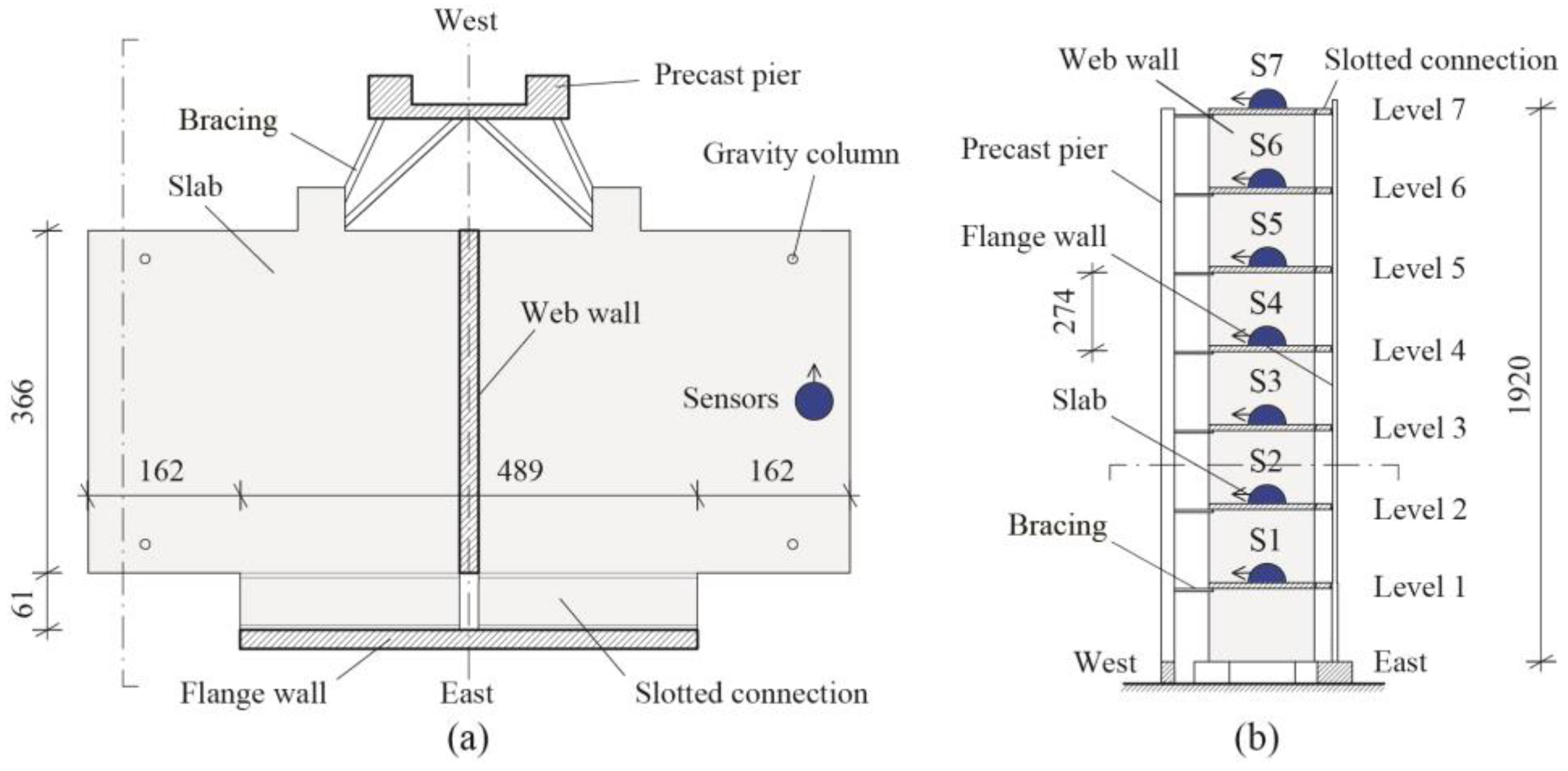
The case study of this paper is a full-scale slice of a seven-story reinforced concrete building with cantilever structural walls acting as the lateral-force-resisting system, which was tested on a shaking table at the University of California, San Diego, through the George E. Brown Jr. Network for Earthquake Engineering Simulation program [
22,
23,
24]. The test structure (
Figure 1) is about 20 m high overall, consisting of two perpendicular walls in elevation (web and flange wall) and a concrete slab at each level. The structure also has an auxiliary post-tensioned column, which provides torsional stability, and four gravity columns that support the slabs at the corners. Geometric details are provided in
Figure 2.
The shaking table tests were designed to progressively damage the building by simulating four historical earthquakes of increasing intensity recorded in Southern California.
Before and after each test with seismic excitation, the structural response of the building was recorded during a white noise excitation of 0.03 g root mean square (RMS) with an amplitude for 8 min and a low amplitude ambient vibration for 3 min. In this study, only the acceleration collected in these “inspection” intervals of 11 min was used and merged into a single dataset with a total duration of 3300 s. Specifically, the first 11 min refer to a reference “undamaged” condition, after which the first seismic excitation (EQ1, i.e., the longitudinal component of the San Fernando earthquake of 1971 recorded at the Van Nuys station) was applied. Subsequently, three intervals of the same length were recorded before and after two medium-intensity earthquakes (EQ2 and EQ3, i.e., the transverse component of the San Fernando earthquake recorded at the Van Nuys station in 1971, and the longitudinal component of the Northridge earthquake recorded at the Woodland Hills Oxnard Boulevard station in 1994, respectively). After EQ3, the bracing system between the slabs of the building and the post-tensioned column was stiffened. The last inspection interval was recorded after a high-intensity 360° excitation (EQ4, i.e., the Northridge earthquake of 1994, recorded at the Sylmar Olive View Med).
During the first three EQs, minor yet increasing damage was observed at the first two levels [
23]. During EQ4, flexure (horizontal) and flexure–shear (inclined) cracks were observed at the first story of the web wall. Moreover, a failure of the lap splice was observed in the web wall on the west side at the bottom of the second story. This failure involved debonding of the longitudinal steel reinforcement bars and the surrounding concrete. For this damage scenario, Moaveni et al. [
23] also identified damage at the fourth level experimentally by using different data series.
The structure was instrumented with 45 accelerometer channels: 29 in the longitudinal direction (three on each floor slab, one on the web wall at mid-height of each story, and one on the pedestal base), 14 in the transversal direction (2 on each floor slab), and 2 in the vertical direction (at the base, on the pedestal). The original data were sampled at 240 Hz. All the datasets are freely available on the DesignSafe online repository [
24,
28].
In this study, only seven acceleration channels were used (i.e., the longitudinal channels on each floor slab, as reported in
Figure 2), which were downsampled to 100 Hz.
The initialization step of the identification process was applied to a signal window consisting of the first 60 s of the dataset collected in the undamaged condition. The Fejér–Korovkin 14 wavelet function and a decomposition order of six were selected to analyze the signal. All the channels were considered in the MAC-based clustering procedure, with a threshold of 0.8, and assigning only consecutive components to the same cluster (see [
9] for more details). In
Figure 3, the filter bank obtained at the end of this process was reported in the frequency domain and superimposed with the frequency spectra of all the channels of the signal used for initialization. Due to its high energy (represented as a solid black circle), only the first mode was selected for further analysis.
Then, the entire dataset (i.e., the acceleration response collected at all the instrumented locations before and after each earthquake) was processed through convolution with the selected bandpass filter to extract only the first modal component from the structural response. The instantaneous frequency and amplitude of the filtered signal were thus evaluated by means of TEO. In this study, the analyses were performed offline. However, the algorithm allows for estimating these quantities onboard each sensor in real-time as new acceleration data is available.
Figure 4 shows an average of the instantaneous frequency of the first vibration mode of the structure computed at all nodes, which was weighted with the relevant instantaneous amplitudes. All seven accelerometers represented in
Figure 2 were considered to obtain this estimate. The overall amplitude, intended as the sum of instantaneous amplitudes evaluated while considering the filtered signal of all nodes, is represented using the color scale (normalized values).
The dashed vertical lines in
Figure 4 represent the occurrence of the four earthquakes described earlier. Each interval delimited by two seismic events is also divided into two parts: The response to 0.03 g of RMS white noise excitation was analyzed in the first 8 min, while low-amplitude ambient vibration was analyzed in the remaining part. This fact is also evident from the plot color, which is typically darker for larger response amplitude values (i.e., in the initial part of each damage scenario).
Figure 4 shows that the identified instantaneous frequency was quite noisy and strongly dependent on amplitude variations, thus presenting abrupt alterations when moving from high to low-amplitude excitation. The dependence of natural frequencies on signal amplitude clearly indicates nonlinear structural behavior [
29].
Figure 4 also shows that changes due to amplitude variations are often more significant than those due to different damage scenarios. This fact makes instantaneous frequency unusable as the only parameter for damage identification.
A computational algorithm was written that simulates online processing in order to apply the procedure proposed in
Section 2, i.e., using a small subset of 2000 couples of frequency–amplitude parameters at a time. The dataset was then updated every 10 s by replacing 1000 frequency–amplitude couples with new incoming identified parameters, as explained in
Section 2.1.
Figure 5 shows the identified instantaneous frequencies and amplitudes of the first modal response evaluated at the 7th floor of the test structure, which are represented as dots in a 2D plane. Here, normalized time is represented as a color bar next to each figure.
In
Figure 5a, the data is represented as extracted, i.e., without any selection criterion. It is possible to observe that some time intervals corresponding to the ambient vibration data sets were only characterized by low-amplitude values. In these parts, the model fitting would be based on a restricted range of amplitudes, which are not representative of the complete structural behavior. In
Figure 5b, the selection criterion proposed in this paper were applied and, indeed, each data set
included samples with a comprehensive set of amplitudes. In
Figure 5c, amplitude-based data sorting was performed, and a median filter of 51 samples was applied, obtaining a
dataset at instant
. This step was performed to de-noise the frequency–amplitude distribution and prepare it for model fitting.
Figure 5d shows the model described in Equation (2), fitted to
datasets reported in
Figure 5c. It is worth noting that the mode values of these distributions shifted in the frequency axis as the damage scenario changed. Therefore, it can be considered a suitable damage-sensitive feature.
Overall,
Figure 5 shows that, in the analyzed case study, the structural behavior in the undamaged configuration was almost linear, as the instantaneous frequencies formed a nearly normal distribution. On the other hand, as the structure experienced damage, lower instantaneous frequencies were identified at high-amplitude instants, which highlighted a softening behavior of the structure. An increasing level on nonlinearity is typically related with damage [
23,
30]. Defining the damage index as the mode of the skew–normal distribution makes it possible to take this concept into account.
Figure 6 shows the mean, variance, and skewness of the models identified on the seventh floor of the test structure, together with the DSF proposed in Equation (7). The mean values of the identified distributions were sensitive to damage and insensitive to amplitude variations. Moreover, variance and skewness indicate the spread and asymmetry of the distribution and are thus linked to structural nonlinearity [
31]. As for variance, the identified value grew with the progressive structural damage and was not dependent on the amplitude level, while skewness showed a sharp increase in the last scenario when the damage level was maximum. The main difference between the feature represented in
Figure 6 (proposed approach) and instantaneous frequencies reported in
Figure 4 (representative of the traditional approach) is that the former was insensitive to the frequency shift due to nonlinearities. In each damage scenario, the DSF was nearly constant, except for a transition interval at the occurrence of earthquakes. This gradual transition was due to updating the frequency–amplitude couples, and its length depended on the number of couples considered for model fitting.
Figure 7 shows the variation of the DSF evaluated at each level of the case study. In this figure, it is possible to observe that the damage index increased with time, except for the scenario after EQ3, in which the impact of retrofit interventions (i.e., stiffening the bracing system) was stronger than the effect of damage. Also,
Figure 8 reports the cumulative amount of detected “positives” (with respect to the initial baseline) over time. The variation reported in
Figure 7 is expressed as the percentage variation shown in Equation (8). The threshold for damage detection was chosen as three times the standard deviation of the baseline set, excluding the outliers (intended as the values exceeding three times the median absolute deviation).
Some inaccuracies (i.e., false positives/negatives) in damage detection were observed for both the undamaged and the damaged conditions and became more frequent at the lower levels of the building.
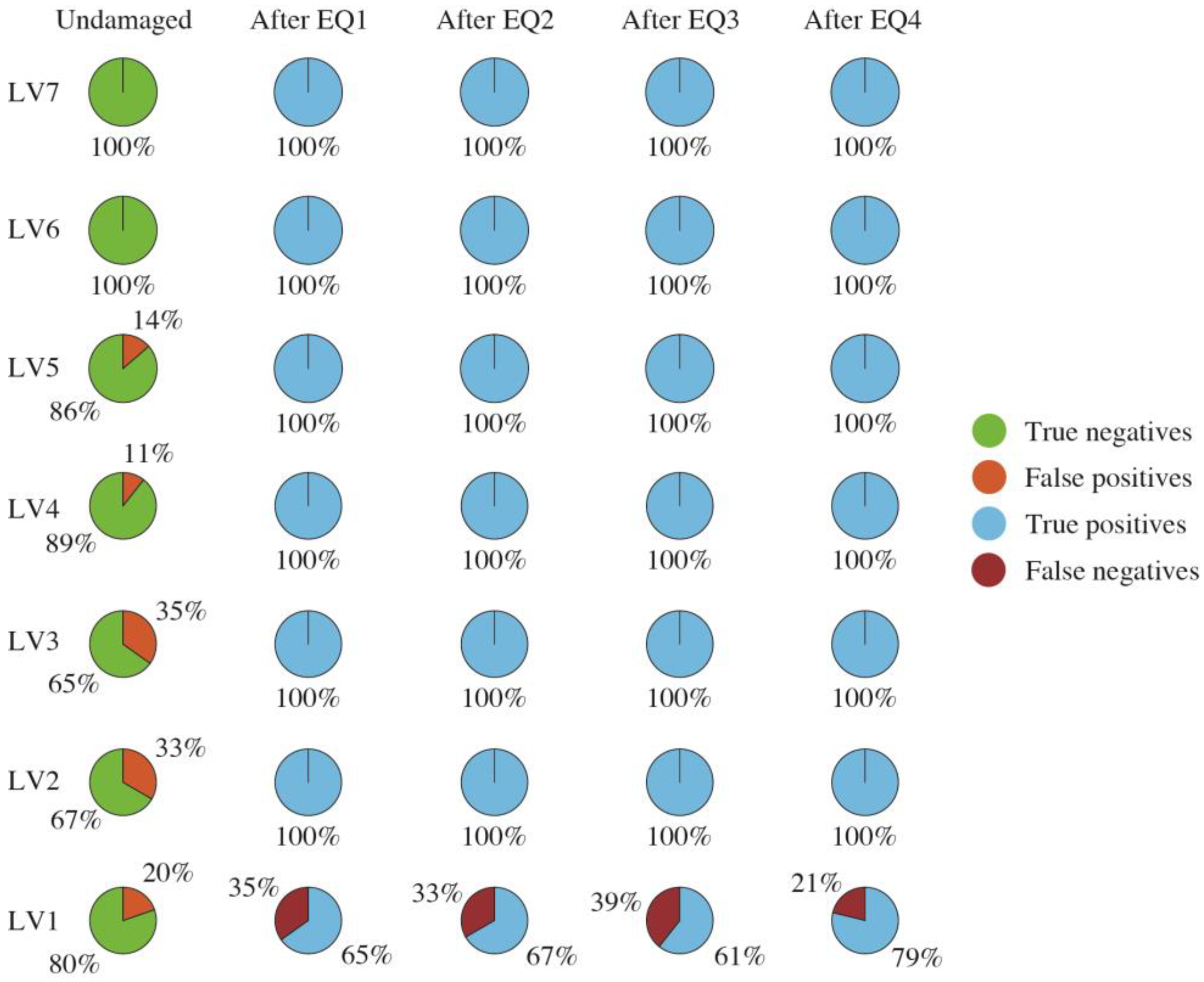
A study about damage detection accuracy was also conducted:
Figure 9 shows the percentage of true/false negatives/positives for each damage scenario and each level of the test structure. On the top floors, damage detection was more accurate. As for levels 6 and 7 (indicated in the figure as LV6 and LV7, respectively), 100% of the tests performed in the undamaged scenario resulted as “negative”, and 100% of the tests performed in all the damage scenarios resulted as “positive”. On the other hand, from levels 2 to 5, the positives were correctly detected at 100%, while some “false positives” were identified in the undamaged scenario. At level 1, a considerable percentage of “false negatives” was detected, making the estimation unreliable. This fact may be due to the low amplitude of the structural response collected at the lower floors, which were affected mainly by noise. However, by analyzing the results from all levels, as is performed in
Figure 8, correct damage detection could be achieved for all scenarios by setting 50% of “positives” as a threshold.
After a centralized initialization for the construction of the analysis filter, the possibility of evaluating the DSF individually at each level brings a considerable advantage for energy efficiency. Indeed, the amount of wirelessly transmitted data can be minimized and only consist of a “positive” notification transmitted when the DSF exceeds the selected threshold. Therefore, the probability that the structure is actually damaged increases when a substantial number of positives are collected at the central monitoring base.
The cumulative number of positives identified depends on the threshold of the damage index. In this application, the threshold was fixed based on the baseline dataset. Therefore, all the following scenarios were identified as “damaged”. It is also possible to initialize the threshold periodically to detect evolving damage. For instance, in this application,
Figure 7 shows that even by updating the threshold after every earthquake, variations in the damage index would have been detected for all scenarios. Specifically, after EQ3, a (negative) variation of the damage index was clearly visible, thus reflecting the retrofit intervention.


