Selection of Response Reduction Factor Considering Resilience Aspect

Abstract

The selection of an adequate response reduction factor (R) in the seismic design of a reinforced concrete building is critical to the building’s seismic response. To construct a robust structure, the R factor should be chosen based on the building’s resilience performance. Since no background was provided for the selection of R factors, the study focuses on the right selection of R factors in relation to the building’s functionality, performance level, and resilience. In this study, a high-rise building with multiple R factors (R = 3, 4, 5, and 6) is developed. Five potential recovery paths (RP-1 to RP-5) that matched the realistic scenario were used to estimate the building’s functionality. The building was subjected to uni and bi-directional loadings, and two design levels, Design Basic Earthquake (DBE) and Maximum Considered Earthquake were used to monitor the building’s response. According to the findings, a decrease in the lateral design force with the highest R results in a high ductility requirement and a substantial loss of resilience. The maximum R factor can be recommended under uni-directional loading up to 6, in which the building’s resilience is almost 50%, whereas under bi-directional loading and taking the recommended R factor decreased from 6 to 4.

1. Introduction

The seismic forces that are put on the buildings have been typically far higher when compared to those that were taken into account during design. A response reduction factor is used by several design codes to account for a building’s non-linear reaction (R). Each nation’s codes recommend using the R factor to reduce the building’s elastic response. In ASCE-7 [1], Eurocode-8 [2], and Indian Standard IS: 1893-2016 [3], the factor ‘R’ is referred to as the “response modification coefficient”, the “behaviour factor”, and the “response reduction factor”, respectively. To lower the seismic stresses and move the building near the inelastic range, the majority of structures employ response reduction factors. Therefore, a larger amount of deformation is required for the structure to disperse energy.

Numerous research work has been conducted to estimate the response reduction factor’s (R) influence on the seismic response of the structure. The response reduction factor (R) mentioned is significantly greater than the actual scenario according to Indian Standard [4]. The revised response reduction factor (R) value with regard to the earthquake series was discovered [5]. The conclusion shows that the adjusted R is less than the intended R. In a study by Djamal Yahmi et al. [6] to determine the impact of storey height and column/beam capacity ratio on behaviour factor (q) for steel special moment resistant frame (SMRF), it was discovered that the low-rise construction q factor recommended by Eurocode-8 is too low. By using non-linear pushover analysis, Kruti Tamboli and Amin. J. A [7] conducted a study to determine the impact of bracing system layout on the R factor. They found that the placement of bracing/shear walls in alternate bays increases the R factor. The R value proposed by the country codes is on the upper level, according to research by Nishanth, M. et al. [8] that aims to analyse the appropriate R value using non-linear pushover analysis with consideration of non-linearity in terms of geometrical orientation, storey height, etc. To determine the building’s seismic reaction, a non-linear pushover analysis was used where the results demonstrate that the response reduction factor “R” is influenced by the load path, ductility factor, and beam column strength ratio [9]. The impact of vertical linkages in braced frames on the response reduction factor in accordance with seismic demand and capacity was determined [10]. Non-linear static pushover analysis was used to investigate how soil flexibility affected the R factor, time period, and overall performance of the structure [11]. Non-linear time history was performed to conduct a study for medium seismicity, three-story health care facility with varied significance factor (I) values of 1.0, 1.2, 1.4, and 1.5, where the outcome demonstrates that when an important element is higher, the building sustains less damage [12]. The impact of non-uniformity in terms of span and height on the response reduction factor was examined, where the findings suggest that non-uniformity has a significant negative impact on the R value as it relates to height [13]. An investigation was conducted on how changing the building boundary condition affected the R factor [14]. A study was conducted to assess the R factor for bare and steel braced RC framed structures [15]. Kappos [16] carried out research to identify the many variables, such as ductility and overstrength factor, which influence the behaviour of the building. The parameters necessary to develop the response reduction factor for a framed RC structure were explored by Patel and Shah [17]. For RC members’ structural behaviour, the significance of component wise response reduction was evaluated [18]. The non-linear behaviour of the building at increasing ground motion levels is determined by the R factor [19]. The cracking coefficient was used in the analysis to account for strength degradation in terms of stiffness, and its impact on the building’s resilience was noticed by S Prasanth and Goutam Ghosh [20]. A shift in the seismic design acceleration spectrum happens as a result of an imbalance in the ambient circumstances, affecting the building’s operation. Prasanth S and Goutam Ghosh [21] assessed the seismic resilience of an existing building using a variety of design acceleration spectrums. For the pre-disaster response assessment, the stakeholders/decision-makers can utilise the computational platform, which includes a hybrid model developed by Sebastiano Marasco et al. [22] to anticipate damage loss and resilience at a large scale without addressing recovery. A study was conducted to determine how four different ground motions would affect a five-story structure with limited ductility and a soft storey mechanism’s operation and performance [23]. A quantitative method for assessing earthquake resilience in the healthcare society was also put forth by Gian Paolo Cimellaro et al. [24] along with the concept. The importance of repair downtime for structural loss recovery was emphasised by the author Gian Paolo Cimellaro et al. [23] because it combines social, environmental, and structural losses for a specific ground motion with various hazards for the hospital community system. According to Gian Paolo Cimellaro et al. [25], theoretical formulae have been developed to quantify the direct and indirect losses brought on by structural-socio degradation. In a study by Stephen Hudson [26], the need for reliable infrastructure was underlined, along with resilience-based design concepts and recommendations for designing infrastructure with adequate resilience. The resilience-based approach was used, according to Daniel Gallagher and Heather Cruickshank [27], even during extreme weather events. The three solutions proposed by Mark Grigorian and Mozhgan Kamizi [28] for constructing durable or long-lasting earthquake-efficient moment frames were replaceable energy-dissipating moment connections, energy-dissipating grade beams, and a hybrid rocking-stepping core. A bridge-specific fragility model was created by Jazalyn Dukes et al. [29] using Monte Carlo simulation and logistic regression as a design tool to support the performance-based strategy for enhancing the seismic resilience of bridges. A number of studies [30,31,32] were carried out to estimate the risk of collapse of common structures planned using different design codes. However, the majority of these experiments use two-dimensional (2D) building models that have been subjected to a single direction of seismic forces.

A greater R factor results in higher detailing costs, whereas a lower R causes overestimation of the design base shear, which results in larger member cross sections. The major literature gap from the previous studies, though several studies were performed in evaluating and using realistic R in design, was silent about based on what aspects of the R factor should have to be selected apart from the seismicity zone and type of structure. Hence the study tries to create a methodology that links R factor selection with building resilience with consideration of the recovery process. The study emphasises the most crucial component in the choice of R factors, which is the term called resilience. A proper recovery strategy for post-earthquake occurrences benefits from the selection of R factors based on resilience. The study highlights that resilience, performance level, and ductility demand must be taken into account in the selection of the R factor together with the examination of directional effect because many country code laws are quiet in these areas.

The study aims to emphasise the need for resilience consideration in the selection of the R factor for high-rise buildings. The proposed methodology/design concept can be adopted irrespective of the building type.

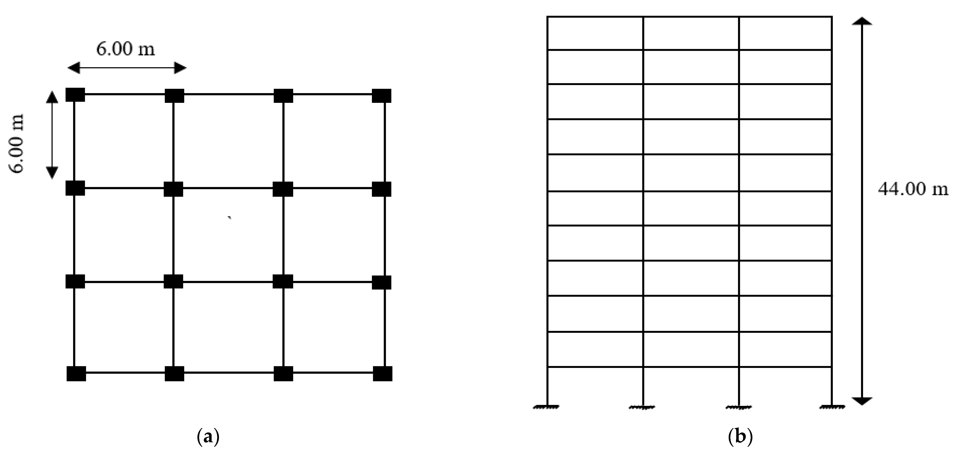
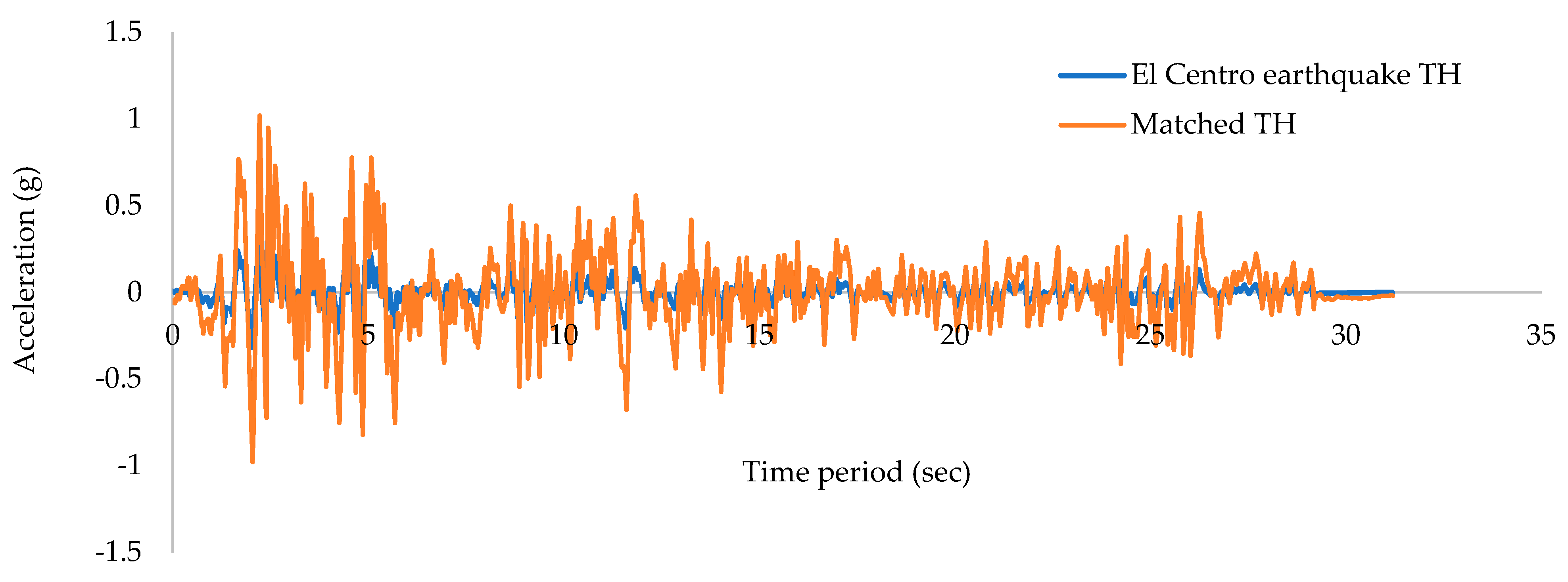
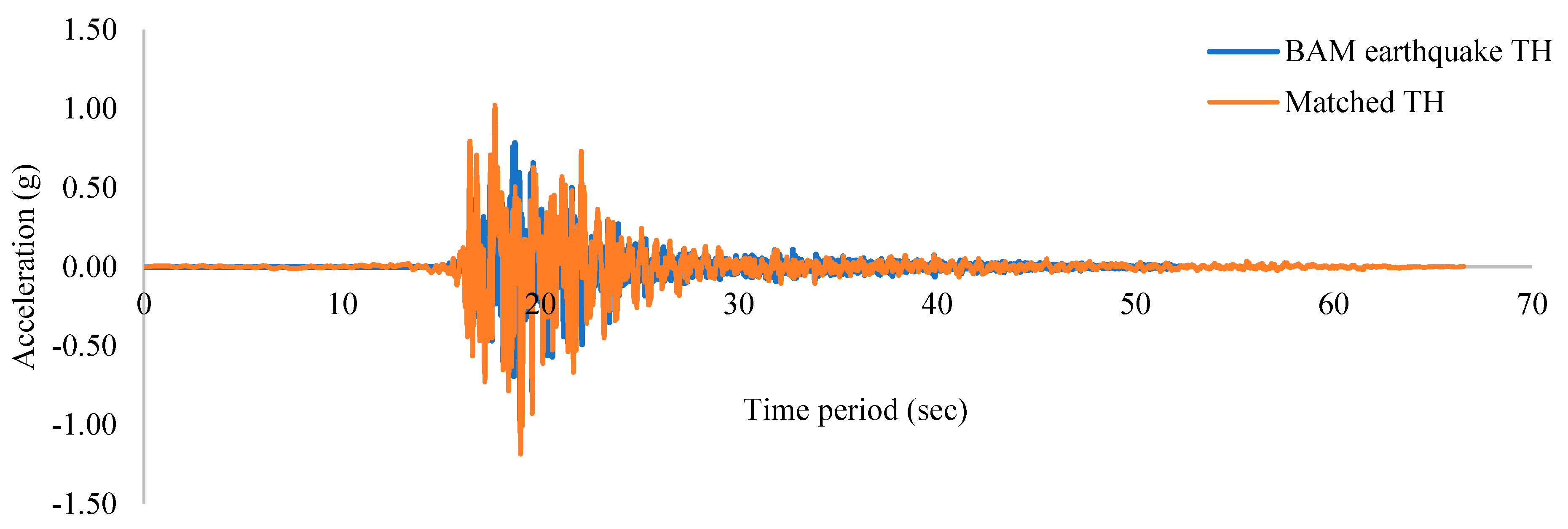
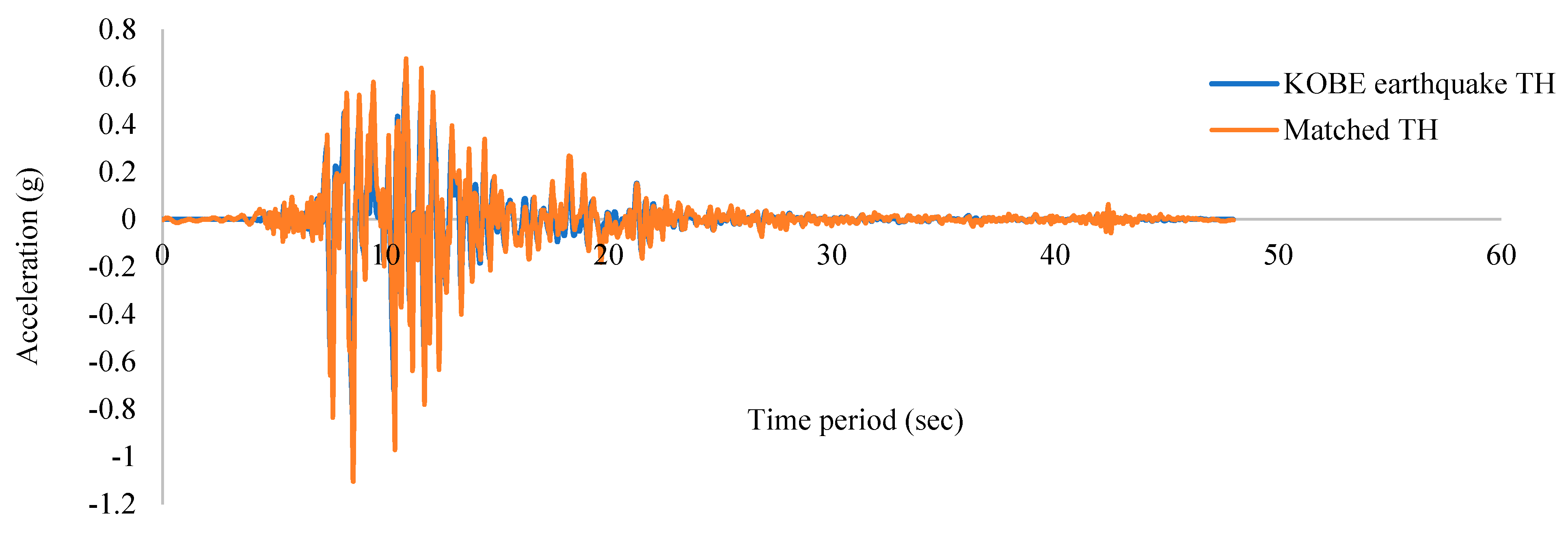
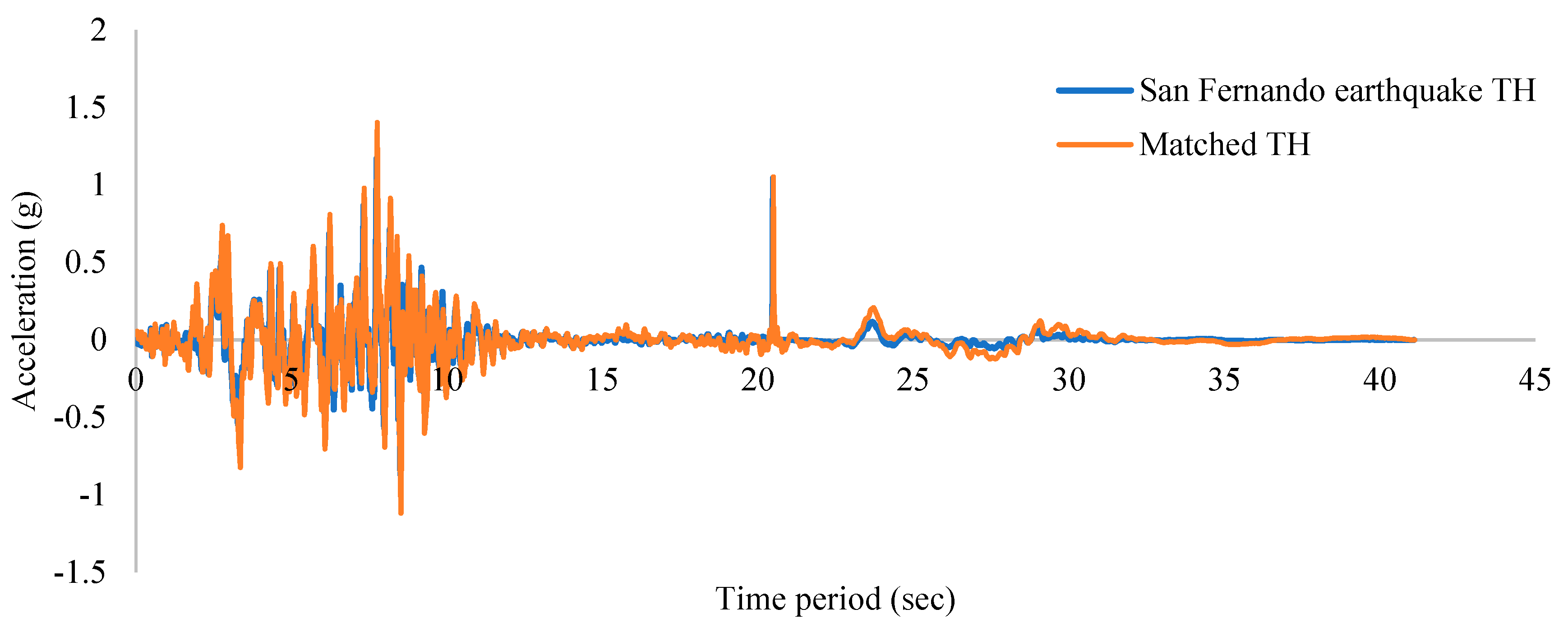
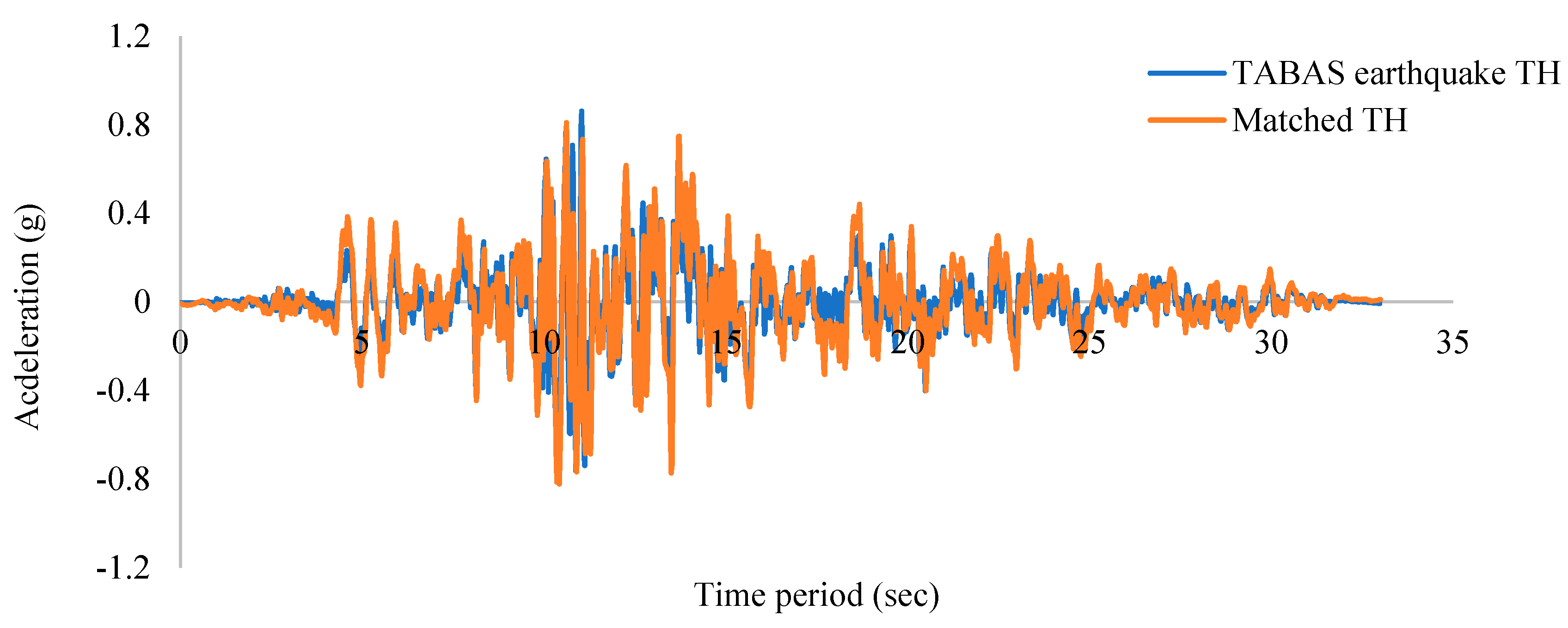
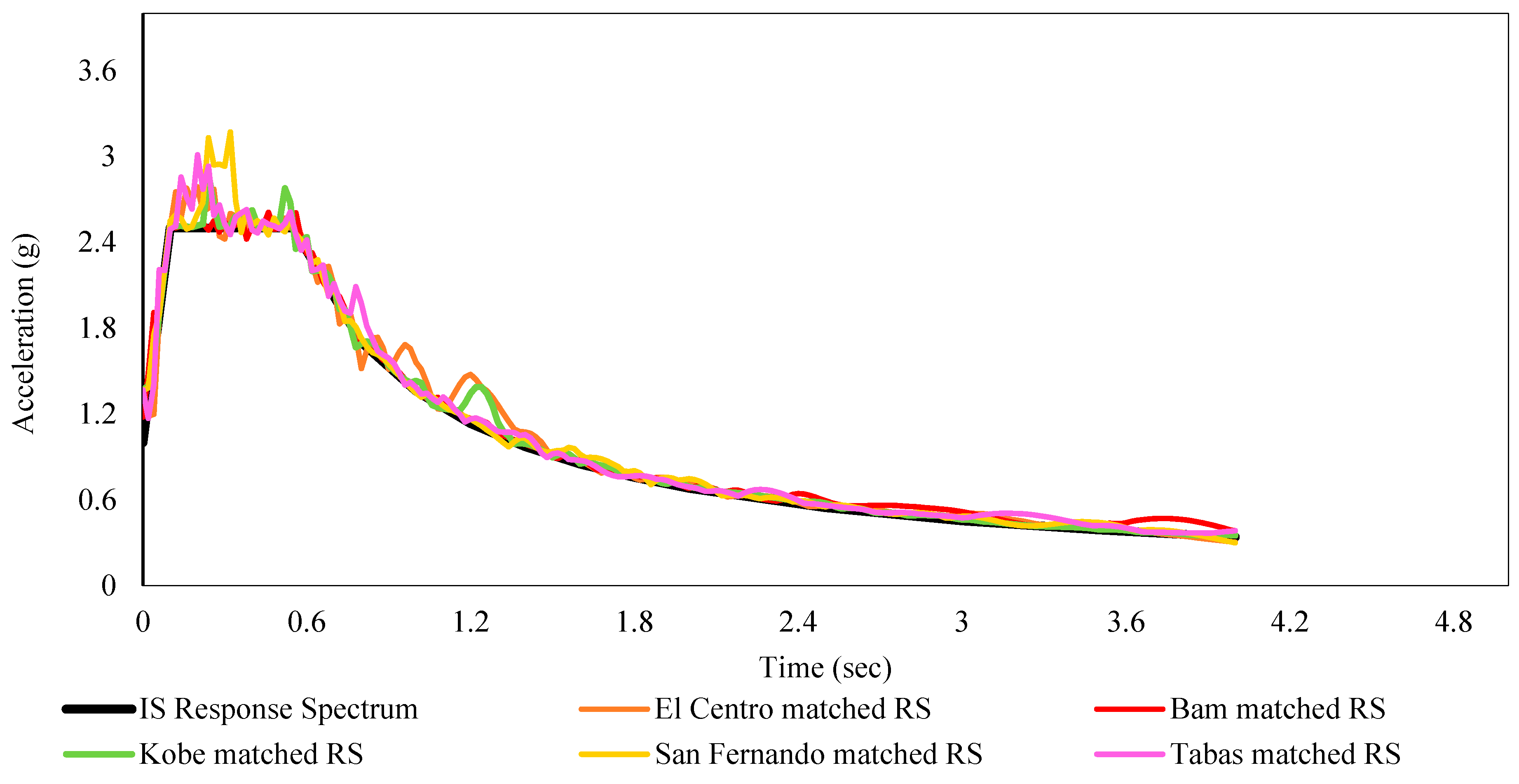
2. Building Information and Ground Motions Considered

For this study, a G+10 storey high-rise symmetrical building was taken into consideration. The structure is 18 × 18 m in area, with a total height of 44 m and a storey height of 4 m (Figure 1). The three-dimensional view is shown in Figure 2, which displays the natural axes in the x, y and z-direction of the building along with a rigid diaphragm with various member levels.

The building has been modelled based on IS: 456-2000. The wall is 230 mm thick on the outer periphery, and a floor finish of 1.5 kN/m² was taken into account. Considerations included the live load of 3 kN/m² and the roof live load of 0.75 kN/m². For beams and columns, respectively, grade M25 and M30 concrete have been taken into consideration. In this study, steel reinforcement with a 500 MPa yield strength was employed. 5% damping with medium (Type II) soil was considered in accordance with IS 1893:2016 (Part-I). In order to study different R factor scenarios (R = 3, 4, 5, and 6), the importance factor (I) was set at 1.5 and the zone factor (Z) at 0.36. For each occurrence of R, the performance of the buildings was evaluated in relation to two design levels, namely the DBE and MCE levels. DBE and MCE levels have scale factors of 2.6487 and 5.2974, respectively. El Centro, Kobe, Bam, San Fernando, and Tabas were among the five distinct earthquake ground motions that had an effect on the construction. The ground motion time history information was gathered from the ground motions database of the Pacific Earthquake Engineering Research (PEER) centre. The minimum number of accelerograms required for the time history analysis is different in different codes. For example, a minimum of three accelerograms is required for two-dimensional analyses of buildings according to ASCE (2010) and IS: 1893 (2016), while five accelerograms are required by CHBDC (2010) and AASHTO (2010). Hence in this study, five accelerograms were used. The selected ground motions belong to near-fault earthquakes. The selected ground motion records are made compatible with respect to the target response spectrum (Indian Standard) and were considered in the study. In order to make the ground motion consistent with the IS codal response spectrum, compatible time history (TH) data were discovered (Figure 3, Figure 4, Figure 5, Figure 6 and Figure 7). Figure 8 depicts the response spectrum that was matched to the IS codal response spectrum.

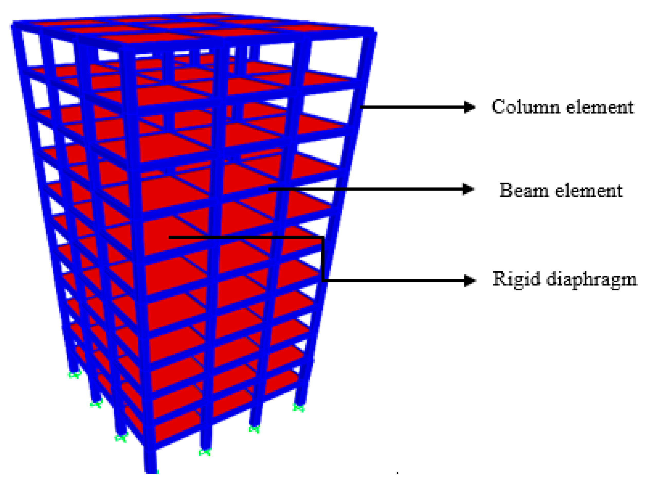
3. Analysis and Design of the Building

The building has been modelled and designed as per IS: 456-2000 using SAP2000 [33], considering various R factors accounting for various parameters such as the building’s occupancy/performance level, ductility demand and seismic resilience. The ductile detailing was provided in the design as per IS: 13920-2016 by using confined concrete. The structural details of concrete members are shown in

Table 1. Structural information of the building corresponds to case-I.

Case No.	Structural Members		Cross Section		Area of Longitudinal Reinforcement ‘Ast’ (mm2)
			Width (mm)	Depth (mm)	Top	Bottom
I (R = 3)	Beam		300	600	1183	1183
	Column	C1 (upto 8 m)	720	720	24–25Ø
		C2	550	550	20–20Ø

,

Table 2. Structural information of the building corresponds to case-II.

Case No.	Structural Members		Cross Section		Area of Longitudinal Reinforcement ‘Ast’ (mm2)
			Width (mm)	Depth (mm)	Top	Bottom
II (R = 4)	Beam		300	510	1183	1183
	Column	C1 (upto 12 m)	680	680	20–25Ø
		C2	520	520	12–25Ø

,

Table 3. Structural information of the building corresponds to case-III.

Case No.	Structural Members		Cross Section		Area of Longitudinal Reinforcement ‘Ast’ (mm2)
			Width (mm)	Depth (mm)	Top	Bottom
III (R = 5)	Beam		300	480	603	603
	Column	C1 (upto 20 m)	620	620	12–25Ø
		C2	480	480	12–20Ø

and

Table 4. Structural information of the building corresponds to case-IV.

Case No.	Structural Members		Cross Section		Area of Longitudinal Reinforcement ‘Ast’ (mm2)
			Width (mm)	Depth (mm)	Top	Bottom
IV (R = 6)	Beam		300	460	603	603
	Column	C1 (upto 20 m)	560	560	16–20Ø
		C2	420	420	12–20Ø

. The matched time history was used for the analysis. The LTHA was performed to find the actual demand of the member forces. The critical beams and columns were found for each design level. The building undergoes NLTHA, from which the actual capacity of the structural concrete members (beams and columns) was found from hinge frame properties. The building was designed with a view to maintaining demand and capacity balance. As the critical columns are on the bottom floors, the cross sections are kept higher than the remaining floor and also in view of the economical design in such tall buildings. Though the extremal columns are more critical, the uniform cross-section was maintained (Table 1, Table 2, Table 3 and Table 4). The maximum reinforcement of columns considered for building cases I, II, III and IV are 2.27%, 2.07%, 1.60% and 1.53%, respectively. The reinforcement percentage was fixed in such a way that the building did not cross the collapse level. Figure 9 shows the traditional concept of seismic design philosophy where the building is designed to withstand moderate intensity shaking with minimum damage loss and severe intensity shaking with more structural damage but with collapse prevention. Figure 10 describes the general concept behind the study. An RC building designed with various R factors shows different functionality losses, which affects the recovery process. This, in turn, affects the resilience of the building. To emphasise this concept, the schematic representation is shown in Figure 10. The detailed description of the limits, such as T_RE, T_LC and t_OE, were explained later in resilience Section 5.

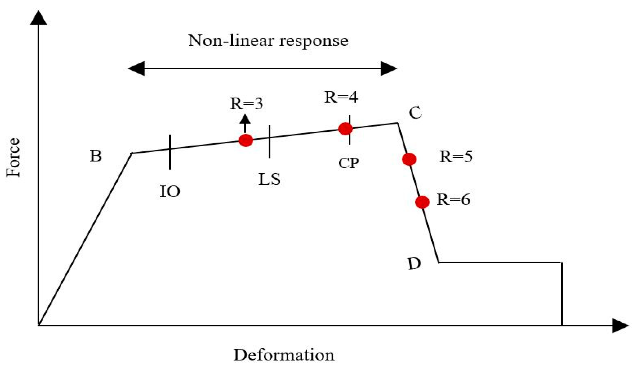
3.1. Non-Linear Time History Analysis (NLTHA)

Modelling and non-linear time history analysis were performed using SAP2000 V22 [33]. The collapse phenomenon is the combination of plastic and the dynamic behaviour of the structural members. Though distributed plasticity provides slightly better results, in terms of modelling difficulties, the lumped plastic hinges are assigned as per ASCE 41-17. The plastic hinges were assigned in beams and columns at the starting and end portion of the member. The beam elements were assigned with M3 hinges, whereas for columns, it was P-M2-M3 hinges [34,35]. M3 hinges in the beam element describe the post-yield behaviour corresponding to the major bending axis. P-M2-M3 hinges for the column describe the post-yield behaviour of the column with combined axial and bi-axial bending conditions. The default P-M2-M3 hinge in SAP2000 interpolates the post-yield behaviour using one or more moment-rotation (P-θ) curves, which indicates the relationship between M2 and M3. In the study, the lateral load resisting systems, such as bracings, URM infills etc., were not included. The slab members were provided along with the rigid diaphragm action at each floor level which inhibits the actual behaviour of the building.

The matched ground motion time history (Figure 3, Figure 4, Figure 5, Figure 6 and Figure 7) was used in the analysis. Since the building is symmetrical in plan orientation, the seismic loading was subjected towards the major direction (Ux). In this study, each building case was subjected to unidirectional loading (Ux direction) and bi-directional loading (Ux and Uy) separately. As per IS: 1893-2016, the structure shall be designed for the simultaneous effects due to full design earthquake loading in one horizontal direction plus 30% of the design earthquake load along the other horizontal direction.

Since the El Centro ground motion was more predominant in the previous analysis, the matched El Centro time history data was used for bi-directional loading conditions. The NLTHA was performed for each building case. The seismic load was applied along the longitudinal (Ux) and transverse (Uy) directions simultaneously [36,37,38,39]. Based on the loading conditions, the maximum roof displacement was found by taking the control node on the roof top with respect to the considered design level. The maximum roof displacement was found for each building case under uni- and bi-directional loading conditions (

Table 5. Maximum top roof displacement under uni-directional excitation.

S.No.	Design Level	Maximum Roof Displacement ‘Δu’ (mm)
		Case-I	Case-II	Case-III	Case-IV
1	DBE	216.09	255.86	267.55	297.08
2	MCE	470.69	509.69	649.72	685.82

and

Table 6. Maximum top roof displacement under bi-directional excitation.

S.No.	Design Level	Maximum Roof Displacement ‘Δu’ (mm)
		Case-I	Case-II	Case-III	Case-IV
1	DBE	220.06	268.06	276.98	308.41
2	MCE	474.15	521.48	660.01	696.52

).

Many studies found the behaviour factor/response reduction factors for different types of building with uni-directional loading conditions. In order to represent the response due to the bi-directional effect, the displacement envelope was plotted (Figure 11, Figure 12, Figure 13 and Figure 14) for the maximum R factor at the MCE design level, where the same pattern will be followed in the remaining cases.

The displacement envelope was plotted by finding the top roof. The displacement envelope was developed with a different incidence angle of seismic excitation (0° to 360°) (Figure 11, Figure 12, Figure 13 and Figure 14) to emphasise the seismic response of the building in terms of displacement at bi-directional loading conditions. Both the axes’ title shows the displacement in meters. From Figure 11, Figure 12, Figure 13 and Figure 14, it was noticed that at higher R factors, the bi-directional effect has a significant impact when compared with the building cases having low R factors. This shows at high seismicity conditions with higher R factors, the bi-directional effect plays a predominant role. Hence, in this study, the directional effect (uni-directional and bi-directional loading) was accounted for to assess the building’s performance.

3.1.1. Ductility Demand Estimation for Each Case of the Building

Ductility demand is the essential seismic characteristic. The ductility demand is the ability of the structure to undergo large deformations without collapse for a specified ground motion. It is expressed by a ratio between maximum displacement and yield displacement. For the evaluation of the ductility, the displacements are determined at the control node, which is located at the roof top level. The capacity curves for each building scenario were determined using a PA based on FEMA-440 [40]. The bilinearisation of the capacity curve was performed as per ATC-40 guidelines [41] to find yield and ultimate displacement, which was used to assess the ductility demand of the building in each case. The yield displacement Δy was defined using the secant stiffness connecting the origin and the peak (maximum) displacement. Yield displacement indicates the end of linear elastic behaviour and the beginning of non-linear inelastic behaviour. The maximum displacement Δu was defined as the post peak displacement corresponding to the peak strength. The ratio of ultimate and yield displacement (Δu/Δy) gives the displacement ductility demand of the buildings at each design level. The ductility demand of each building case under uni and bi-directional loading was found (

Table 7. Ductility demand under uni-directional loading.

S.No.	Design Level	Ductility Demand (μD)
		Case-I	Case-II	Case-III	Case-IV
1	DBE	1.17	1.4	1.50	1.71
2	MCE	2.55	2.78	3.63	3.94

and

Table 8. Ductility demand under bi-directional loading.

S.No.	Design Level	Ductility Demand (μD)
		Case-I	Case-II	Case-III	Case-IV
1	DBE	1.19	1.46	1.55	1.77
2	MCE	2.57	2.84	3.69	4.00

).

According to ASCE 41-17 [34], displacement ductility below 2 indicates low ductility requirement, while displacement ductility greater than 4 indicates high ductility demand. According to Table 7 and Table 8, each case of building at the DBE design level has a ductility demand below 2 μ_D under both uni-directional and bi-directional loading circumstances. This demonstrates that at the DBE level, the building has a low ductility need, which is feasible. At the MCE design level, the building has a ductility demand of nearly 4 μ_D at R= 5 and 6. This means that the higher the R, the greater the ductility demand. It was also observed that the building under bi-directional loading experiences slightly higher ductility demand when compared with uni-directional loading. Though the amount of variation is not significant, the impact on building response can be noted in terms of higher roof displacement and ductility demand.

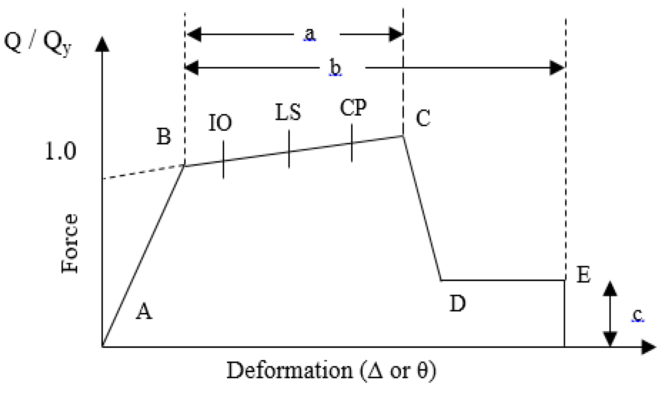
3.1.2. Assessment of Building’s Performance

The performance level indicates the functional attributes of a building considering safety and utility against designed criteria. Non-linear time history analysis (NLTHA) was performed to assess the performance of the building. The building experiences three types of performance levels, namely Immediate Occupancy (IO) level, Life Safety (LS) level and Collapse Prevention (CP) level. The Immediate Occupancy (IO) level indicates only limited structural damage. Life Safety (LS) indicates that significant damage has occurred, but the structure remains in a non-collapse state. Collapse Prevention (CP) denotes that the structure is on the verge of experiencing partial or total collapse. From Figure 15, if the building lies in A–B performance level, it shows that the building is in the elastic range (A–B level). If the building reaches B–C level, it shows that the building’s performance is in the strain hardening region. The performance level C–D shows that the structure starts approaching the collapse range with reduced resistance towards seismic force. Level E shows final resistance loss. In the study, the inter storey drift ratio (IDR) has been checked but not considered as a major parameter since the current study mainly focused on damage loss ratios in accordance with spectral displacement rather than IDR. Hence, based on spectral displacement, the performance level in each case was determined.

The performance level was determined using the force-deformation curve (Figure 15) in conjunction with the performance point’s location and hinge formation. According to pushover analysis, the demand and capacity curves cross at a location known as the performance point, which is where they intersect. The performance level is determined by where that point on the capacity curve lies in the Acceleration Displacement Response Spectrum (ADRS) format. Based on the hinge formation at the conclusion of the ground motion, the performance level for NLTHA was identified. For each building case, the performance level was discovered with respect to each design level.

Table 9. Variation in performance level under uni-directional loading.

S.No.	Design Level	Performance Level
		Case-I	Case-II	Case-III	Case-IV
1	DBE	IO	IO	IO to LS	IO to LS
2	MCE	IO to LS	LS to CP	CP to C	CP to C

and

Table 10. Variation in performance level under bi-directional loading.

S.No.	Design Level	Performance Level
		Case-I	Case-II	Case-III	Case-IV
1	DBE	IO	IO	IO to LS	IO to LS
2	MCE	IO to LS	CP	C to D	C to D

display the performance level based on NLTHA for both uni-directional and bi-directional loading circumstances. The schematic representation of the location of the performance point based on directional loading is shown in Figure 16 and Figure 17. For the study, different limit state parameters can be used, such as ductility, inter storey drift etc.

Table 9 and Table 10 show that the building’s performance/occupancy level has been impacted by the change in R factors under both loading conditions. Under both directional loading situations, the building with R = 3 experiences an IO level at the DBE design level, while with R equal to 6, it approaches the IO-LS level. Although directional loading has no impact on the DBE design level, significant performance level variation was seen at the MCE level.

Under unidirectional loading, the building is located at IO to LS, LS to CP, CP to C, and CP to C at R equal to 3, 4, 5, and 6, respectively, at the MCE design level. The building’s performance level with bi-directional loading is IO-LS level at R = 3, CP level at R = 4, C–D level at R = 5, and C–D level at R = 6. This structural behaviour was not found in the situation of uni-directional loads where the building is located at the CP to C level (Table 9). It demonstrates that taking into account the bi-directional effect reduced the building’s performance level, particularly at larger R factors.

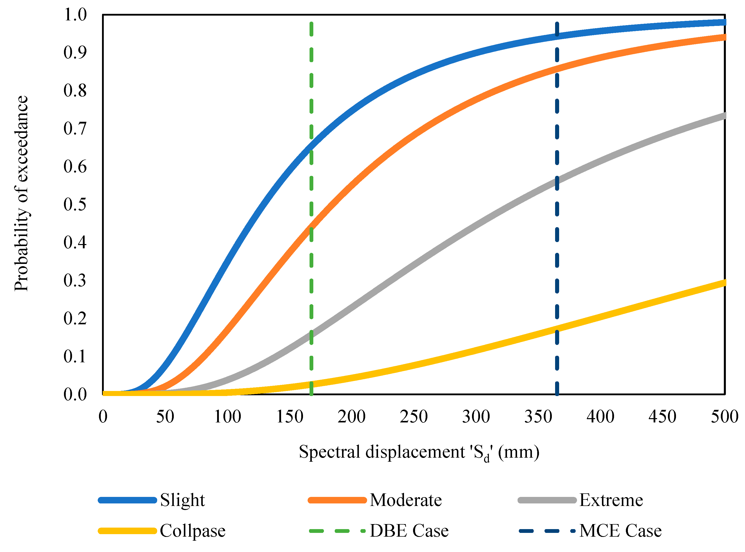
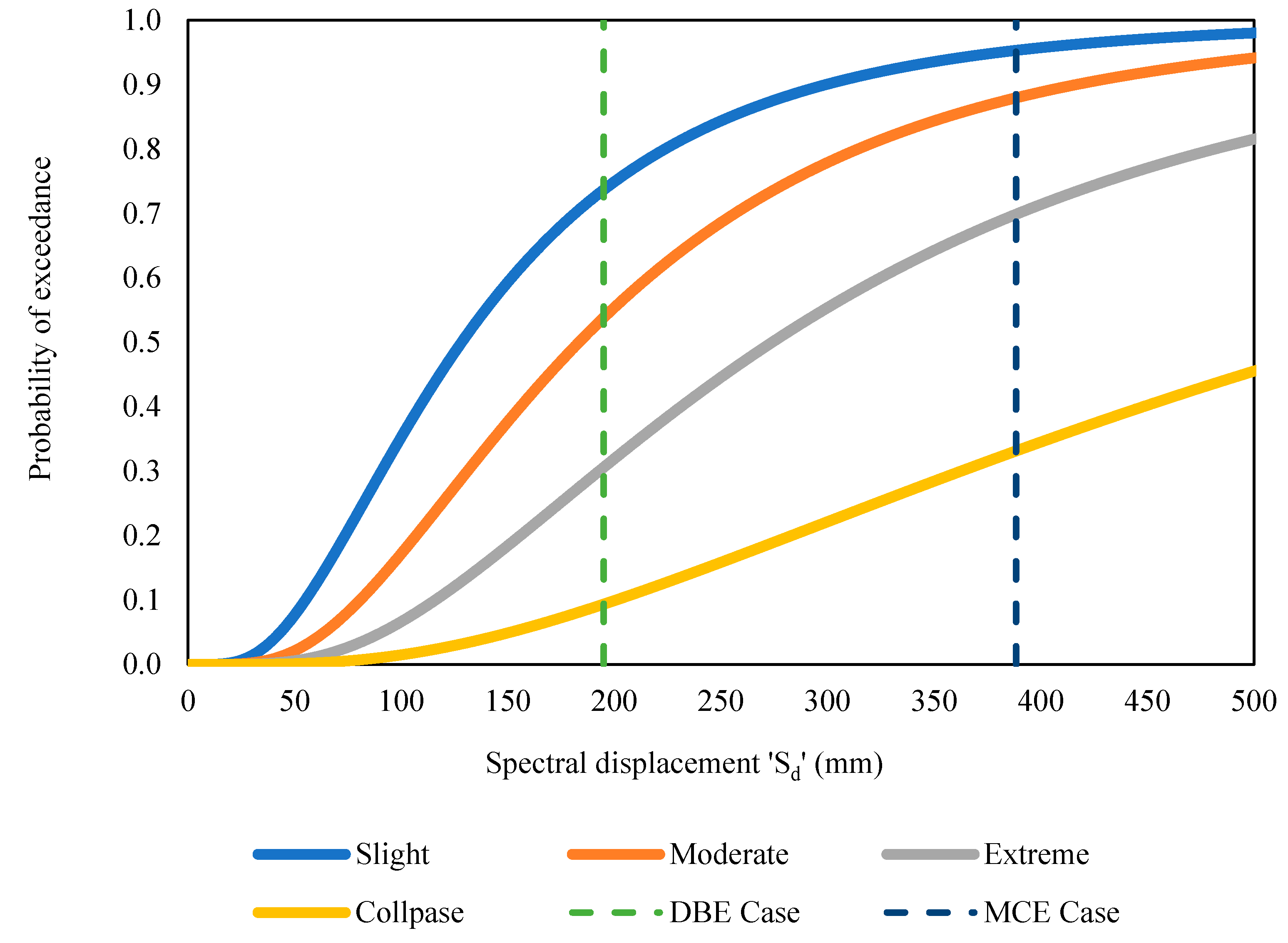
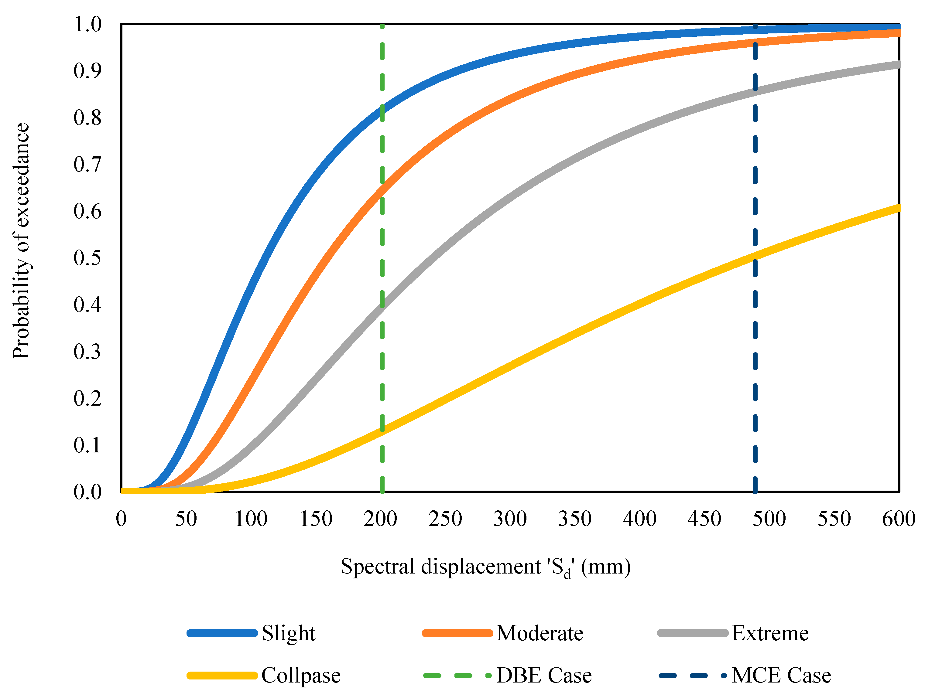
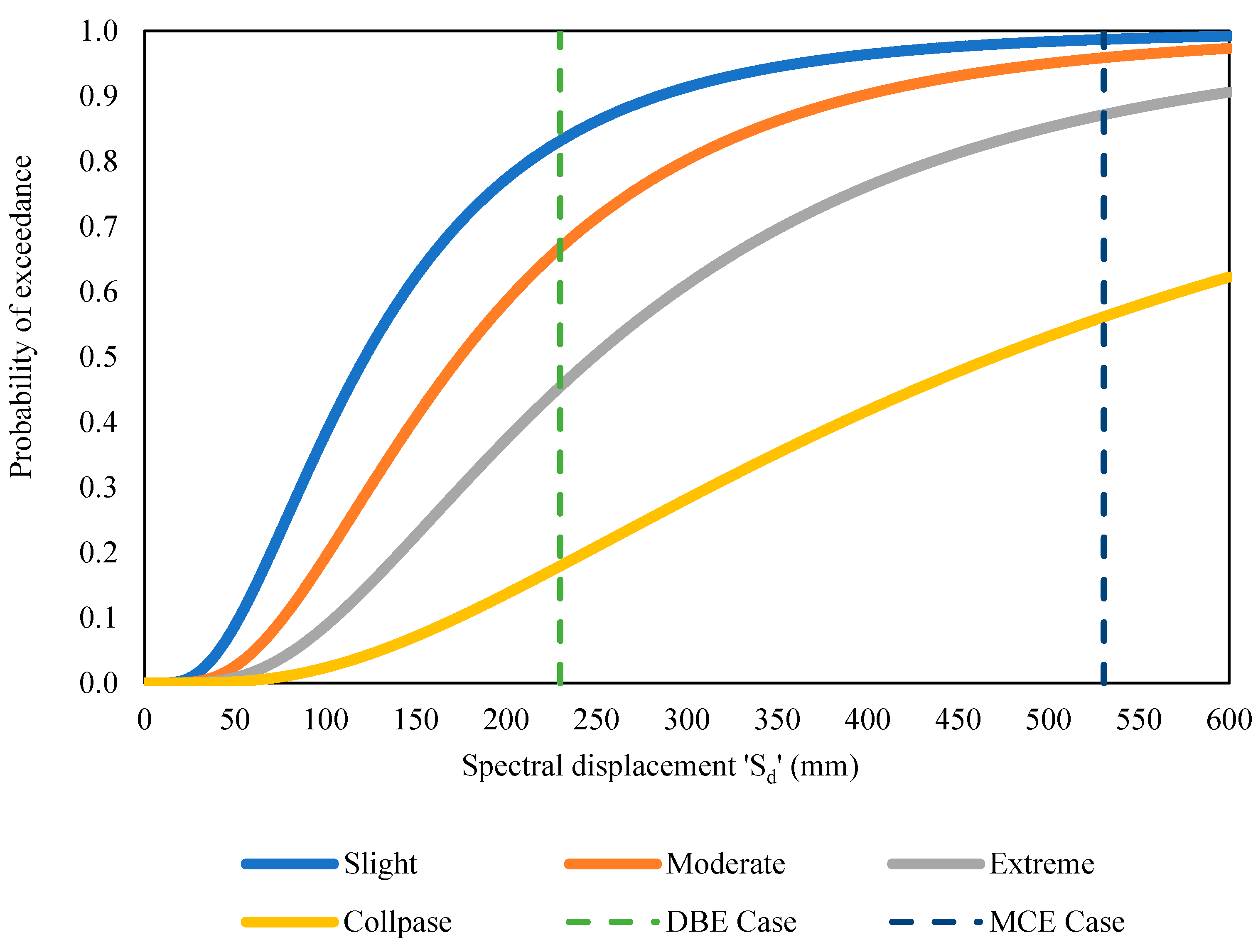
4. Seismic Vulnerability Assessment

The likelihood of exceeding each damage condition, namely slight, moderate, extreme, and collapse, was calculated using the HAZUS technique [42]. Equation (1) was used to calculate the damage probability.

$$P\left(\raisebox{1ex}{$ds$}\!\left/ \!\raisebox{-1ex}{$S_d$}\right.\right)=\varphi \left[\frac{1}{{\beta }_{ds}}\ln \left(\raisebox{1ex}{$S_d$}\!\left/ \!\raisebox{-1ex}{$S_{d,ds}$}\right.\right)\right]$$

(1)

With respect to the first mode (considered as 1), MPF and k, roof top denote the mode participation factor and modal amplitude at the roof top, respectively. Meanwhile, represents the mode shape coefficient, while Wi denotes floor weight at each storey level.

The yield (S_dy) and ultimate (S_du) displacement was determined by bilinearization from the capacity curve derived from the pushover study in accordance with ATC-40 criteria [41]. The equation suggested by Barbat et al. (2006) was utilised to determine the damage state threshold. The spectral displacement (S_d) has been calculated from the maximum top roof displacement with the help of below mentioned formulae;

$$S_d=\left[\frac{{\mathsf{\Delta }}_{rooftop}}{{\varphi }_{k,rooftop}\ast MPF}\right]$$

(2)

$$MPF=\left(\frac{{\displaystyle \sum _{i=1}^n{W}_i{\varphi }_{iK}}}{{\displaystyle \sum _{i=1}^n{W}_i{({\varphi }_{iK})}^2}}\right)$$

(3)

By creating fragility/vulnerability curves with regard to spectral displacement, it was possible to determine the likelihood of exceeding (Figure 18, Figure 19, Figure 20 and Figure 21). The chance of exceeding the vulnerability in terms of the fragility curve on the y-axis and spectral displacement (S_d) on the x-axis were plotted. The y-axis ordinates range from 0 to 1, which represents the probability of reaching a given damage level or state from 0% to 100%. The probability that the building may sustain various damages was calculated using fragility curves.

Damage Loss Assessment

Buildings’ structural and non-structural damages were included in the direct economic loss, whereas indirect economic loss is determined by moving costs, lost income, etc. The study’s primary focus is on direct economic costs related to structural disruption. The loss ratio was found using Equation (4).

$$L_D={\displaystyle \sum P_E}(DS=K)\times r_K$$

(4)

K is the building’s damage state, P_E(DS = K) is the discrete damage probability that the building was in the damaged state at the time of the occurrence, and r_K is the damage ratio for each damaged state as extracted from the HAZUS MR4 technical documentation [42]. From which the discrete damage probability was found.

The direct damage loss ratio was evaluated for each building case at each design level under uni and bi-directional loading conditions (

Table 11. Direct damage loss ratio under uni-directional loading.

S.No.	Design Level	Direct Economic Loss Ratio (LD)
		Case-I	Case-II	Case-III	Case-IV
1	DBE	0.265	0.376	0.459	0.501
2	MCE	0.610	0.705	0.830	0.847

and

Table 12. Direct damage loss ratio under bi-directional loading.

S.No.	Design Level	Direct Economic Loss Ratio (LD)
		Case-I	Case-II	Case-III	Case-IV
1	DBE	0.273	0.399	0.477	0.520
2	MCE	0.613	0.714	0.834	0.852

). The damage loss ratio is higher in the case of a higher R factor, which was due to high ductility demand. Though there was not much difference in damage loss ratio when compared with uni and bi-directional loading conditions, the bi-directional effect shows a slightly higher damage loss ratio which affects the building’s functionality.

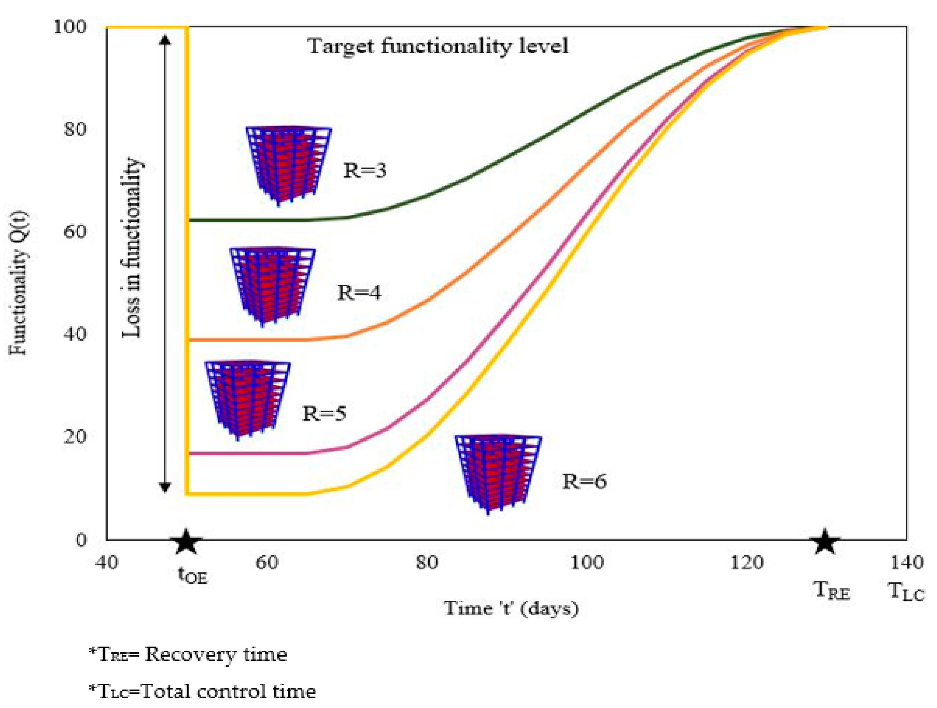
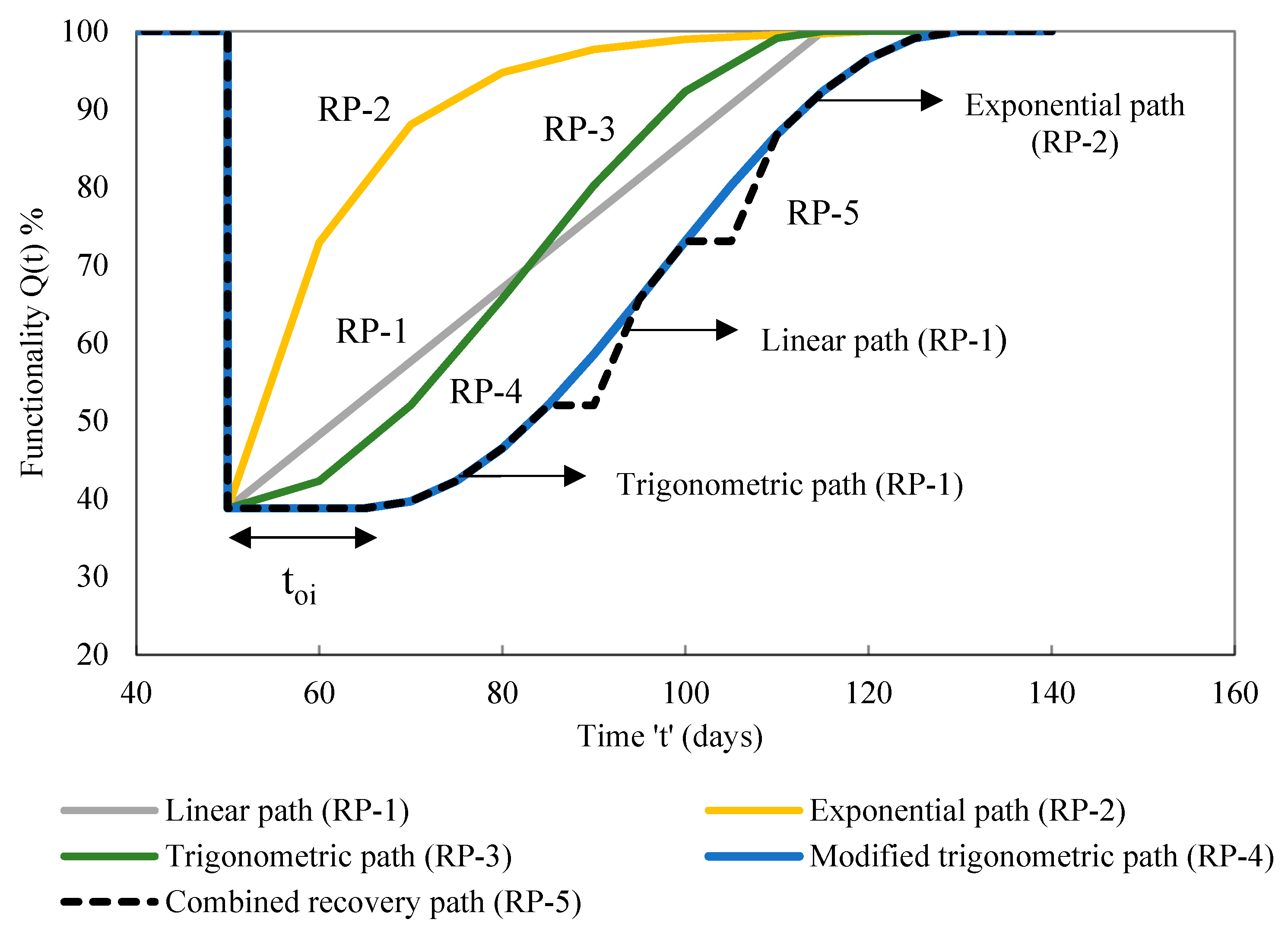
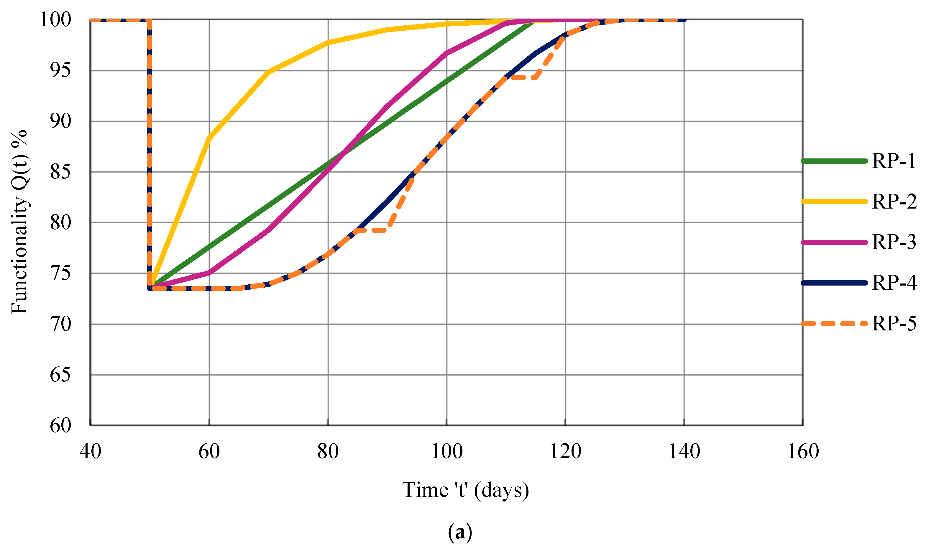
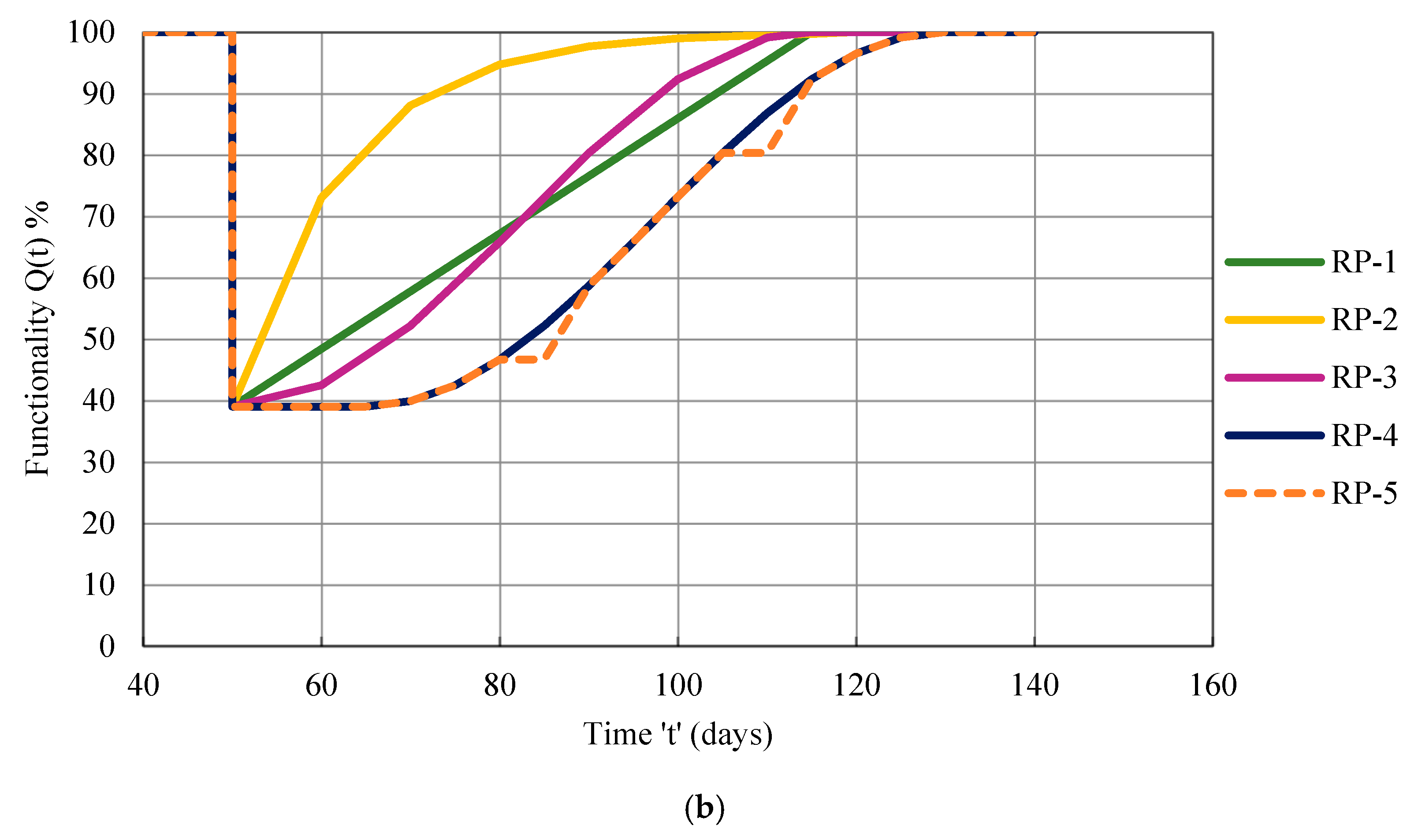
5. Resilience Estimation

Resilience is about preserving and restoring functionality linked to building performance as measured by the amount of time taken to recover back to its target functionality. The functionality curve was found using three analytical recovery models proposed by Michel Bruneau et al. (2003) [43]. The functionality defines the occupancy condition of the building. The newly constructed building is 100% functional. After the occurrence of seismic events, the building gets damaged, which leads to further examination before occupation/use of the building. Resilience is about preserving and restoring functionality linked to building performance as measured by the amount of time taken to recover back to its target functionality. In addition to the three traditional recovery patterns—linear, exponential, and trigonometric—two modified recovery paths based on real-world scenarios were adopted. Using Equation (5), the functionality curve and resilience were discovered.

Functionality:

$$Q(t)=1-\left.\left\{L\left(I,T_{RE}\right)\times \left[H\left(t-t_{OE}\right)-H\left(t-\left(t_{OE}+T_{RE}\right)\right)\right]\times f_{rec}\left(t,t_{OE},T_{RE}\right)\right.\right\}$$

(5)

The time of occurrence of a seismic event is denoted as ‘t_OE’, recovery time as ‘T_RE’ and H( ) is denoted as the Heaviside step function. In this study, t_OE is assumed as 50 days, and a total recovery time of 65 days with a total control time period (T_LC) of 140 days was assumed for the study [44]. In resilience-based design, the recovery time depends upon the functional type of the structure. As an example, for hospital buildings, the recovery time will be minimal since it has to recover fast. Based on this concept, since a single building was considered in the study, the operational need of the building is the same, and hence the recovery time is kept the same for each case of R. In other words, the recovery time is directly proportional to the functional need of the structure.

The analytical equations for each recovery function are shown below;

Linear function:

$$f_{rec}\left(t,t_{OE},T_{RE}\right)=\left[1-\frac{t-t_{OE}}{T_{RE}}\right]$$

(6)

Exponential function:

$$f_{rec}\left(t,t_{OE},T_{RE}\right)=\exp \left[-\frac{\left(t-t_{OE}\right)\left(\ln 200\right)}{T_{RE}}\right]$$

(7)

Trigonometric function:

$$f_{rec}\left(t,t_{OE},T_{RE}\right)=0.5\left\{1+\cos \left[\mathsf{\Pi }\frac{\left(t-t_{OE}\right)}{T_{RE}}\right]\right\}$$

(8)

The linear function (RP-1) adopts steady progress in functionality, which implies the timely availability of resources. The exponential functions (RP-2) have a higher functionality rate at the initial path, which indicates the high resource inflow at the initial stages, but this is not possible in all situations. The trigonometric functions (RP-3) followed less functionality rate at the beginning, which was due to a lack of resources.

Real-world recovery functions follow their own course based on actual circumstances. Figure 22 illustrates the many recovery pathways that each function takes. The behaviour of the linear functions is consistent, suggesting that the resources are accessible when needed. Although this is not always practical, the exponential functions on the initial route have a higher functionality rate, indicating a big influx of resources at the beginning. The trigonometric functions initially operate at a lower functionality rate when resources are scarce.

The functionality Equation (5) now includes the new argument “toi”. The thought behind the parameter’s inclusion was that, in the case of real-world circumstances, recovery could not begin after a seismic event had happened (Figure 22). Real-world events necessitate thorough damage assessments of the structure, and the recovery procedure is time-consuming. Based on this, the functionality and recovery equation was modified as below;

$$Q(t)=1-\left.\left\{L\left(I,T_{RE}\right)\times \left[H\left(t-t_{OE}-t_{oi}\right)-H\left(t-\left(t_{OE}+T_{RE}\right)-t_{oi}\right)\right]\times f_{rec}\left(t,t_{OE},T_{RE},t_{oi}\right)\right.\right\}$$

(9)

$$f_{rec}\left(t,t_{OE},T_{RE},t_{oi}\right)=0.5\left\{1+\cos \left[\mathsf{\Pi }\frac{\left(t-t_{OE}-t_{oi}\right)}{T_{RE}}\right]\right\}$$

(10)

The new recovery path, known as RP-5, has a recovery profile that uses linear, exponential, and trigonometric recovery patterns (Figure 22). Given a “toi” of 15 days and a 5-day respite, two distinct functional levels were examined for recovery. Based on the idea that an increasing recovery path was not viable in any case, a break in the healing process was implemented.

5.1. Resilience of Each Building Case under Uni-Directional Loading

For each design level, the functionality curves were created (Figure 23, Figure 24, Figure 25 and Figure 26) with respect to various recovery paths under unidirectional loading conditions. The area below and above the functioning demonstrates the building’s resilience and loss of resilience (LOR). Utilising the software Origin, the curve’s area was evaluated [45]. Five recovery functions at each design level’s resilience were discovered (Table 9, Table 10, Table 11 and Table 12).

In relation to considered design levels for the case-I building, Figure 23a,b displays the various functionality curves, which were plotted considering five recovery functions. A decline in functionality was observed at the time of the earthquake event occurrence (on the 50th day). The building functionality decreases from 100% to 73.50% and 39.00%, respectively, at DBE and MCE design levels. At the DBE and MCE design levels, the functionality loss was estimated to be 26.50% and 61.00%, respectively. This demonstrates that functionality was significantly reduced at the higher design level (MCE) due to a significant increase in the damage loss ratio than at the DBE design level.

The building’s functionality curves at each considered design level for the case-II building are shown in Figure 24a,b. The fall in the building functionality has been estimated to be 62.40% and 30% at DBE and MCE design levels, respectively, at the time of occurrence of the earthquake event (on the 50th day). At the design level of DBE and MCE levels, the functionality loss was estimated to be 37.60% and 70.50%, respectively.

The various functionality curves corresponding to the case-III building were developed at both design levels (Figure 25a,b). The functionality at the DBE and MCE design levels, respectively, decreases from 100% to 54.10% and 17.01% at the occurrence of an earthquake event (on the 50th day). At DBE and MCE design levels, the loss in the building functionality was assessed to be 45.90% and 82.99%, respectively.

Figure 26 depicts the functionality curves corresponding to both considered design levels for Case-IV Building (a and b). When a disaster event (seismic) occurs (on the 50th day), the functionality with respect to DBE and MCE design levels was reduced from 100% to 49.90% and 15.25%, respectively. At the DBE and MCE design levels, the loss in the building functionality has been estimated to be 50.10% and 84.75%, respectively. In Figure 23, Figure 24, Figure 25 and Figure 26, the area under and above the functioning curves depict, respectively, the building’s seismic resilience and loss of resilience (LOR). Utilising the software Origin, the curve’s area was discovered.

The seismic resilience of each building case corresponding to the considered design level was estimated under five various recovery paths (

Table 13. Seismic resilience of the building corresponds to case-I (R = 3).

S.No.	Case No.	Design Level	Resilience (%)
			RP-1	RP-2	RP-3	RP-4	RP-5
1	I (R = 3)	DBE	86.75	95.37	87.69	84.26	83.93
2		MCE	69.5	88.77	71.69	63.77	63.02

,

Table 14. Seismic resilience of the building corresponds to case-II (R = 4).

S.No.	Case No.	Design Level	Resilience (%)
			RP-1	RP-2	RP-3	RP-4	RP-5
1	II (R = 4)	DBE	81.2	93.08	82.55	77.67	77.18
2		MCE	64.75	87.02	67.29	58.13	57.26

,

Table 15. Seismic resilience of the building corresponds to case-III (R = 5).

S.No.	Case No.	Design Level	Resilience (%)
			RP-1	RP-2	RP-3	RP-4	RP-5
1	III (R = 5)	DBE	77.05	91.55	78.7	72.74	72.17
2		MCE	58.51	84.72	61.49	50.71	49.69

and

Table 16. Seismic resilience of the building corresponds to case-IV (R = 6).

S.No.	Case No.	Design Level	Resilience (%)
			RP-1	RP-2	RP-3	RP-4	RP-5
1	IV (R = 6)	DBE	74.95	90.78	76.75	70.24	69.57
2		MCE	57.63	84.39	60.68	49.66	48.53

). Though the exponential recovery path (RP-2) gives higher resilience, it cannot be considered in all real situations due to its high resource inflow at the initial stages which is not possible.

Table 13 shows that the building’s seismic resilience corresponds to DBE design level varies from 83.93% to 86.75% in accordance with the recovery paths considered (RP-1 to RP-5). The resilience continued to decline under the MCE design level. With respect to the MCE design level, seismic resilience ranges from 63.02% to 69.50%. A higher damage economic loss ratio leads to a maximum fall in the resilience of around 24.9% at the MCE design level. Since recovery path RP-2 was not always a practical option, a comparison of the reaming recovery paths was done.

In comparison with the traditional recovery paths [46], the proposed recovery path RP-5 showed about 3–4% and 12–13% lesser seismic resilience at DBE and MCE design levels (RP-1 and RP-3). This resulted from the recovery process’s initial delay in the beginning. Although the resilience at the RP-4 and RP-5 recovery paths did not change significantly, a minor decline in resilience was seen as a result of the break/delay in the recovery process. At the community level (large scale), the break/delay in the recovery process will affect the recovery time and control time period, leading to a significant drop in seismic resilience. The higher Loss of Resilience (LOR), which corresponds to RP-5, was found to be approximately 16.07% and 36.98% for the DBE and MCE design levels, respectively.

The building’s seismic resilience corresponding to DBE design level changes around from 81% to 77% in case-II (Table 14). The resilience continued to decline at the MCE design level. At MCE design level, the resilience ranges around from 65% to 57%. At the DBE and MCE design levels, respectively, the maximum Loss of Resilience (LOR) has been estimated to be around 23% and 43%.

The building’s resilience in case-III (Table 15) ranges from around 77% to 72% at the DBE design level. The seismic resilience ranges from around 59% to 50% at the MCE design level. At both DBE and MCE design levels, the higher possible Loss of Resilience (LOR) has been discovered to be approximately around 28% and 50%, respectively.

The building’s seismic resilience with respect to DBE design level varies around between 75% and 70% in case-IV (Table 16). Resilience at the MCE design level ranges around from 58% to 49%. At DBE and MCE design levels, the high Loss of Resilience (LOR) was discovered to be approximately 30.43% and 51.47%, respectively. When compared to previous building cases, the building that corresponds to case-IV (R equal to 6) exhibits reduced seismic resilience at both design levels. This was brought on by the significant demand for ductility at R = 6 (case-IV building).

5.2. Seismic Resilience of Considered Building Cases Corresponds to Bi-Directional Excitations

The seismic resilience of cases of the building cases subjected to bidirectional loading has been found (

Table 17. Seismic resilience of the building corresponds to case-I (R = 3).

S.No.	Case No.	Design Level	Resilience (%)
			RP-1	RP-2	RP-3	RP-4	RP-5
1	I (R = 3)	DBE	86.35	94.97	87.33	83.79	83.45
2		MCE	69.35	88.72	71.56	63.59	62.79

,

Table 18. Seismic resilience of the building corresponds to case-II (R = 4).

S.No.	Case No.	Design Level	Resilience (%)
			RP-1	RP-2	RP-3	RP-4	RP-5
1	II (R = 4)	DBE	80.05	92.65	81.49	76.30	75.81
2		MCE	64.30	86.86	66.87	57.59	56.64

,

Table 19. Seismic resilience of the building corresponds to case-III (R = 5).

S.No.	Case No.	Design Level	Resilience (%)
			RP-1	RP-2	RP-3	RP-4	RP-5
1	III (R = 5)	DBE	76.15	91.22	77.87	71.67	71.05
2		MCE	58.30	84.47	61.30	50.46	49.35

and

Table 20. Seismic resilience of the building corresponds to case-IV (R = 6).

S.No.	Case No.	Design Level	Resilience (%)
			RP-1	RP-2	RP-3	RP-4	RP-5
1	IV (R = 6)	DBE	74.00	90.43	75.87	69.11	68.44
2		MCE	57.40	84.32	60.47	49.39	48.26

). The comparison of seismic resilience has been made between uni-directional and bi-directional excitations (Figure 14 and Figure 15).

Figure 27 shows that corresponding to DBE design level, the variance in seismic resilience was not statistically significant with bi-directional loading. When compared to unidirectional loading, the seismic resilience under bi-directional excitations has been marginally weaker in all of the considered building cases at the DBE level. Under uni-directional and bi-directional excitation circumstances, the MCE design level showed a similar variance in seismic resilience (Figure 28).

6. Conclusions

The study’s goal was to demonstrate the significance of the response reduction factor in seismic analysis and design in relation to the usefulness and resilience of the building. A G+10 storey reinforced concrete building was exposed to a various number of seismic excitations under uni- and bi-directional loading conditions. The seismic response assessment was conducted with respect to two design levels, such as the DBE and MCE levels. Resilience, ductility demand, and performance/occupancy level variations have been found for the case of the building corresponding to DBE and MCE design levels. These are the key findings from the study.

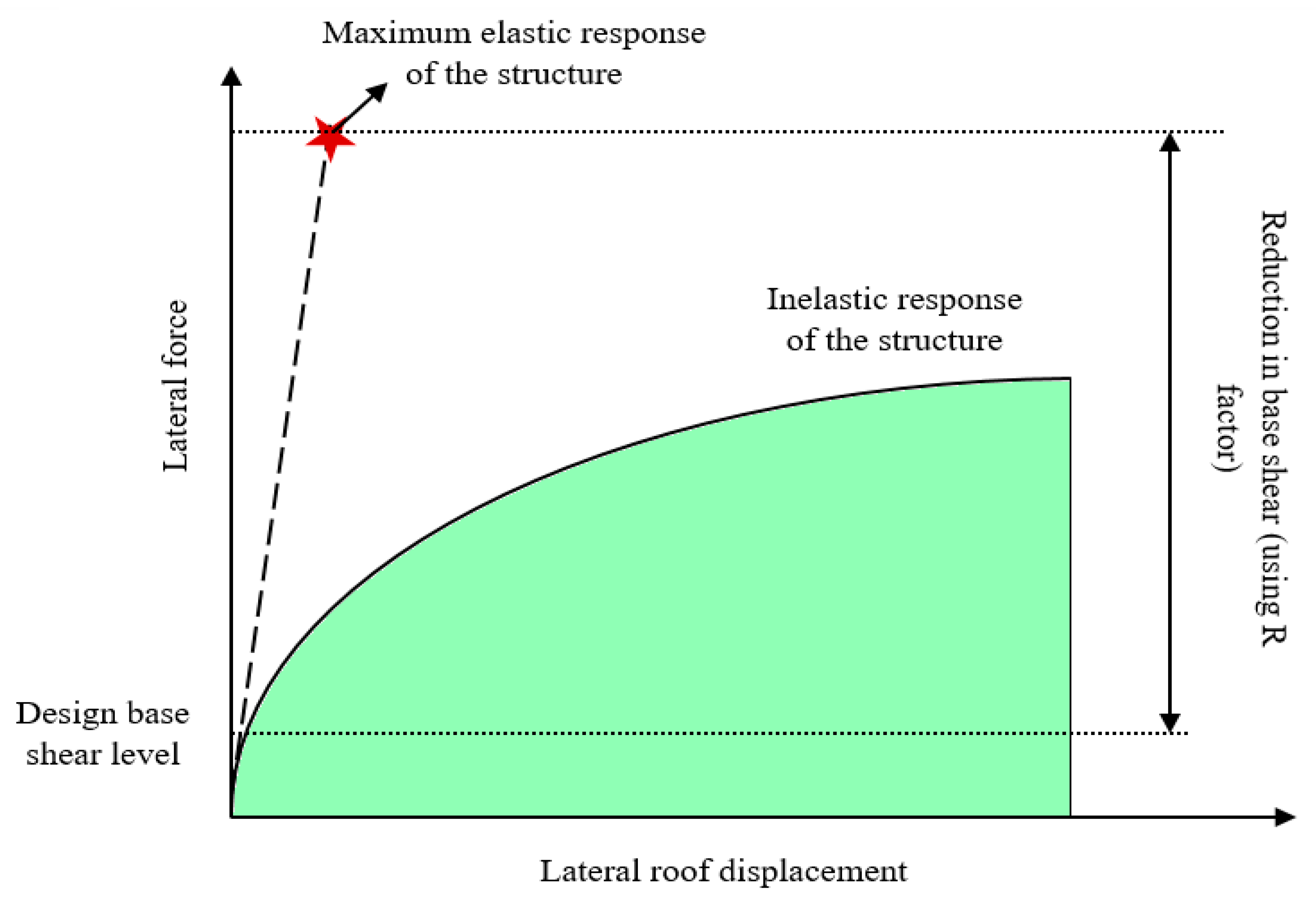
• The findings demonstrate that all building scenarios experience moderate ductility requirements at the DBE design level under uni-directional and bi-directional loading circumstances [47]. At the level of MCE design, the structure approximately meets the high ductility demand for R = 5 and R = 6. This demonstrates that an increase in R factors causes an increase in ductility demand. Buildings with lower ductility demands, such as those in the moderate to high ductility demand range, are generally simpler and more feasible to recover back to the target functionality. This aids in the appropriate selection of R design variables.
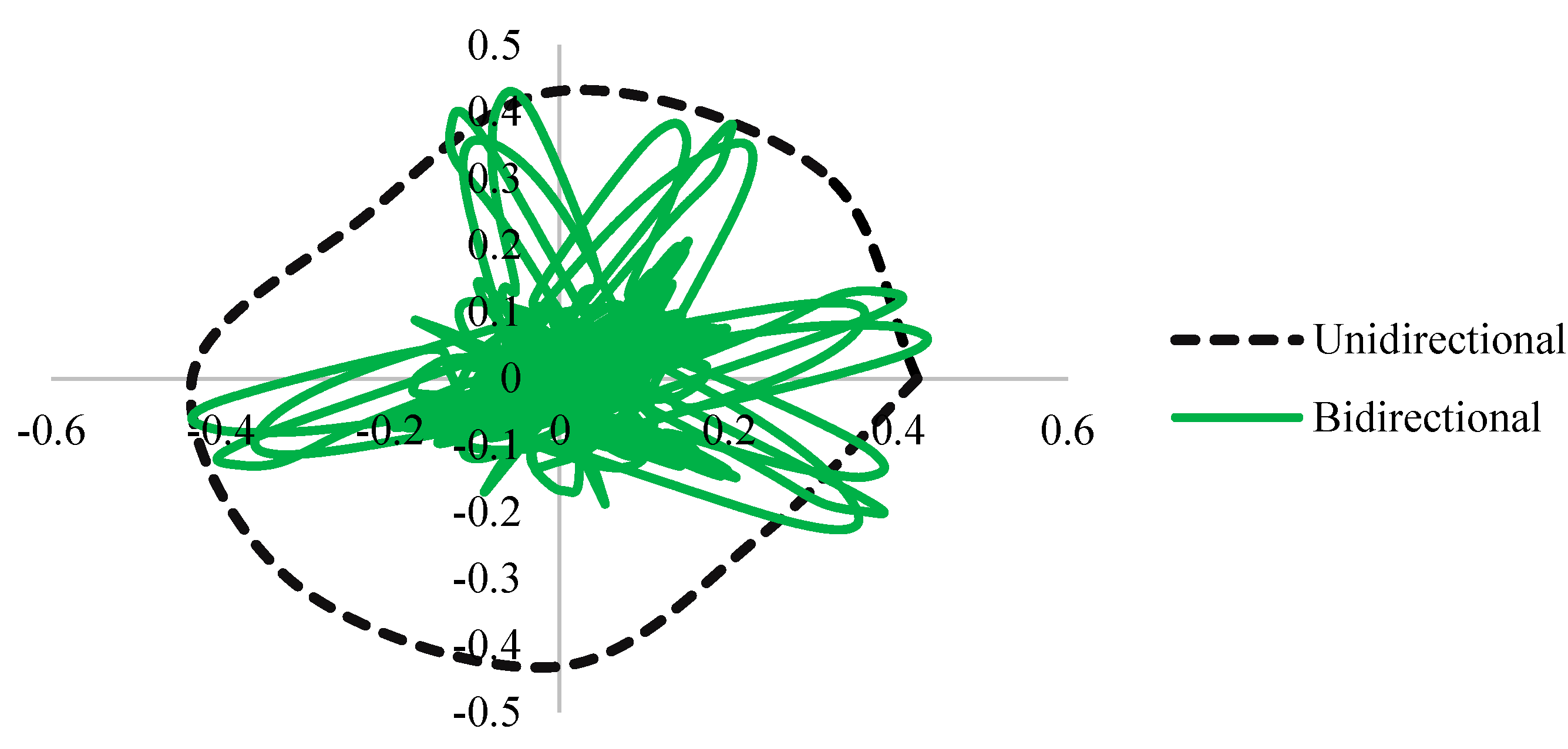
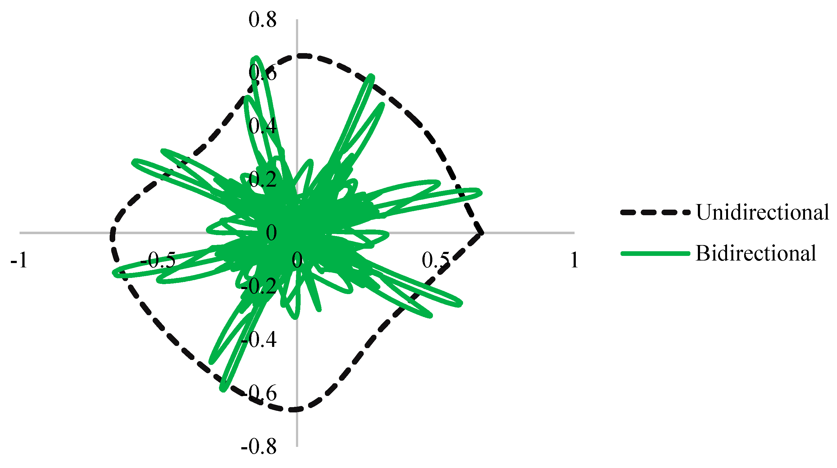
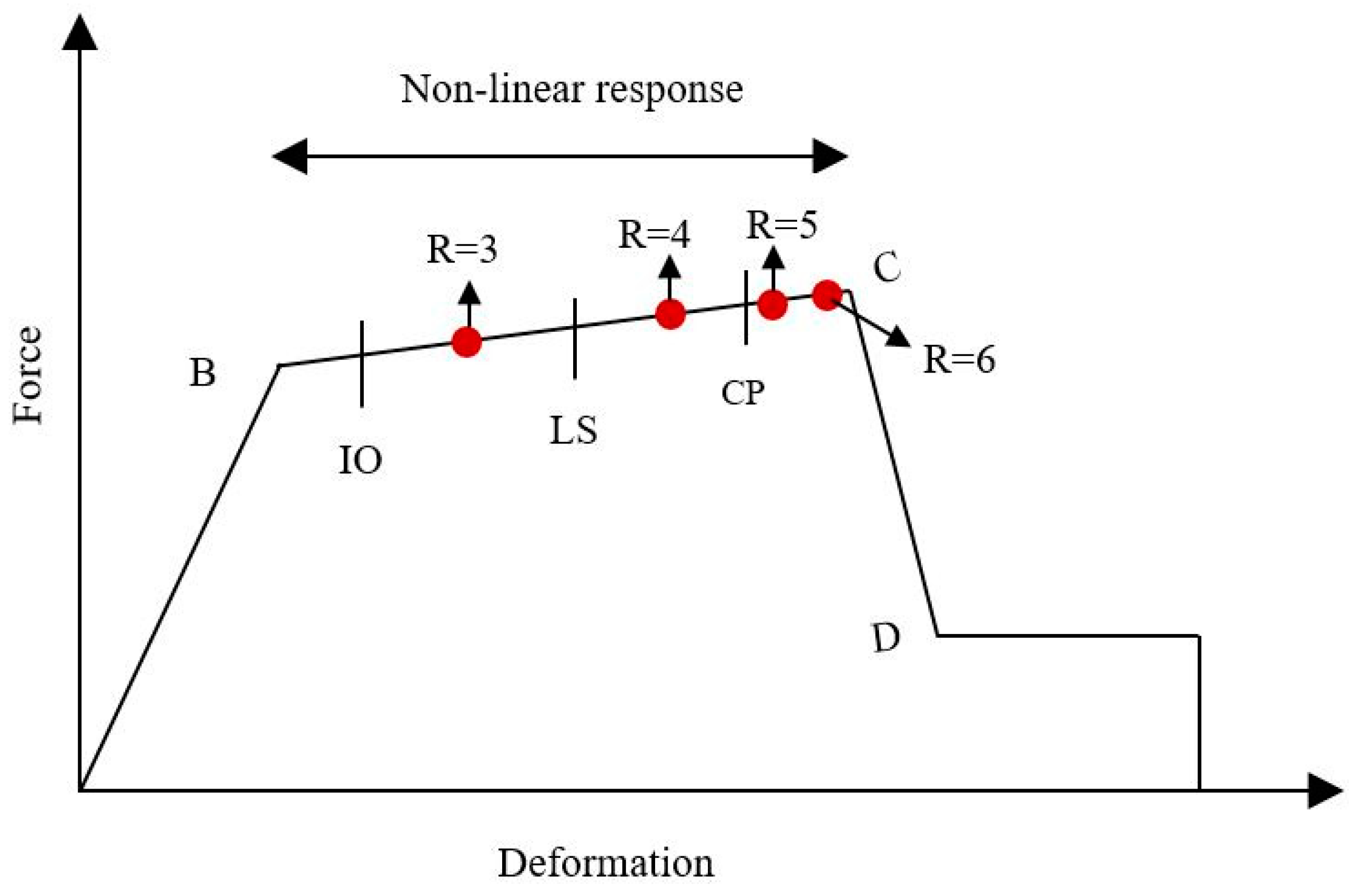
• The outcome demonstrates that a larger R factor has a significant impact on the performance of the building, which was caused by a higher requirement for ductility. The performance level rises from the IO (at R equal to 3 and 4) to the IO-LS level (at R equal to 5 and 6) at the DBE design level. At the MCE design level, the building’s performance level (IO-LS level to CP-C level) varied significantly, going from R = 3 to R = 6. The performance/occupancy level of the building with higher R (R equal to 5 and 6) scenarios under bi-directional loading is at the C-D level. This demonstrates that there is no residual strength in the structure when it reaches its maximum collapse damage level at bi-directional loading conditions. This resulted from a decrease in the transverse member’s contribution to structural stiffness brought on by the influence of bi-directional loading at a higher R factor.
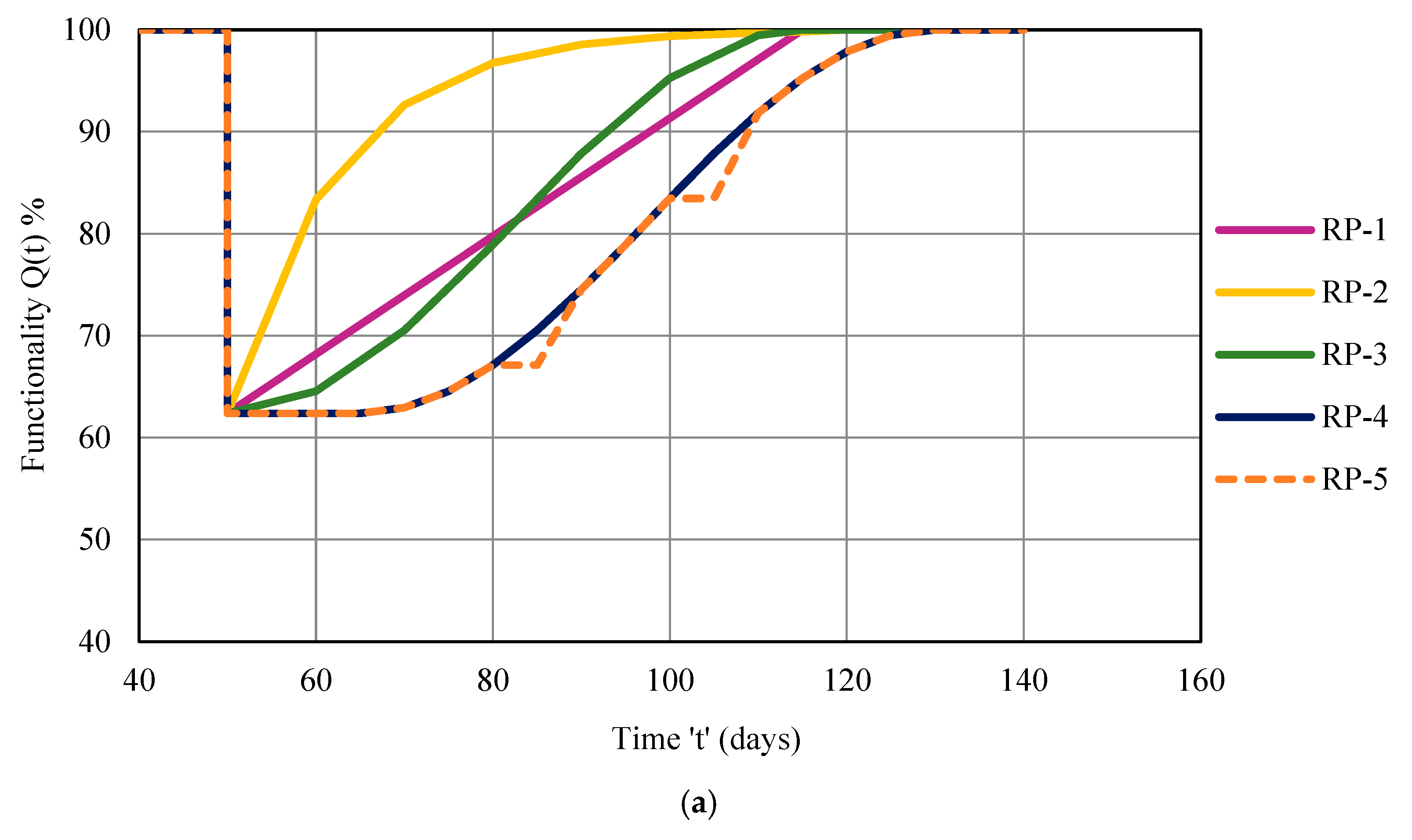
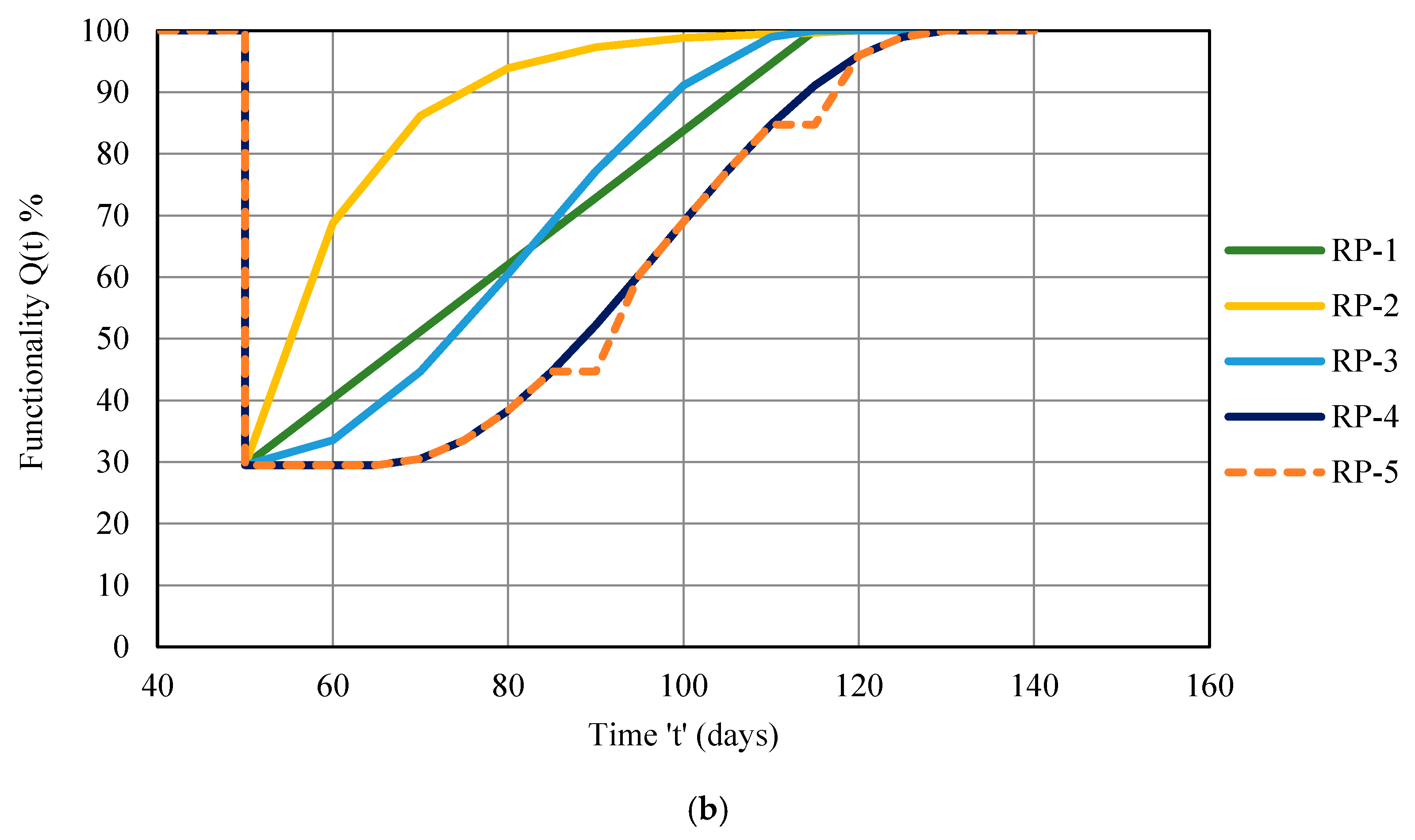
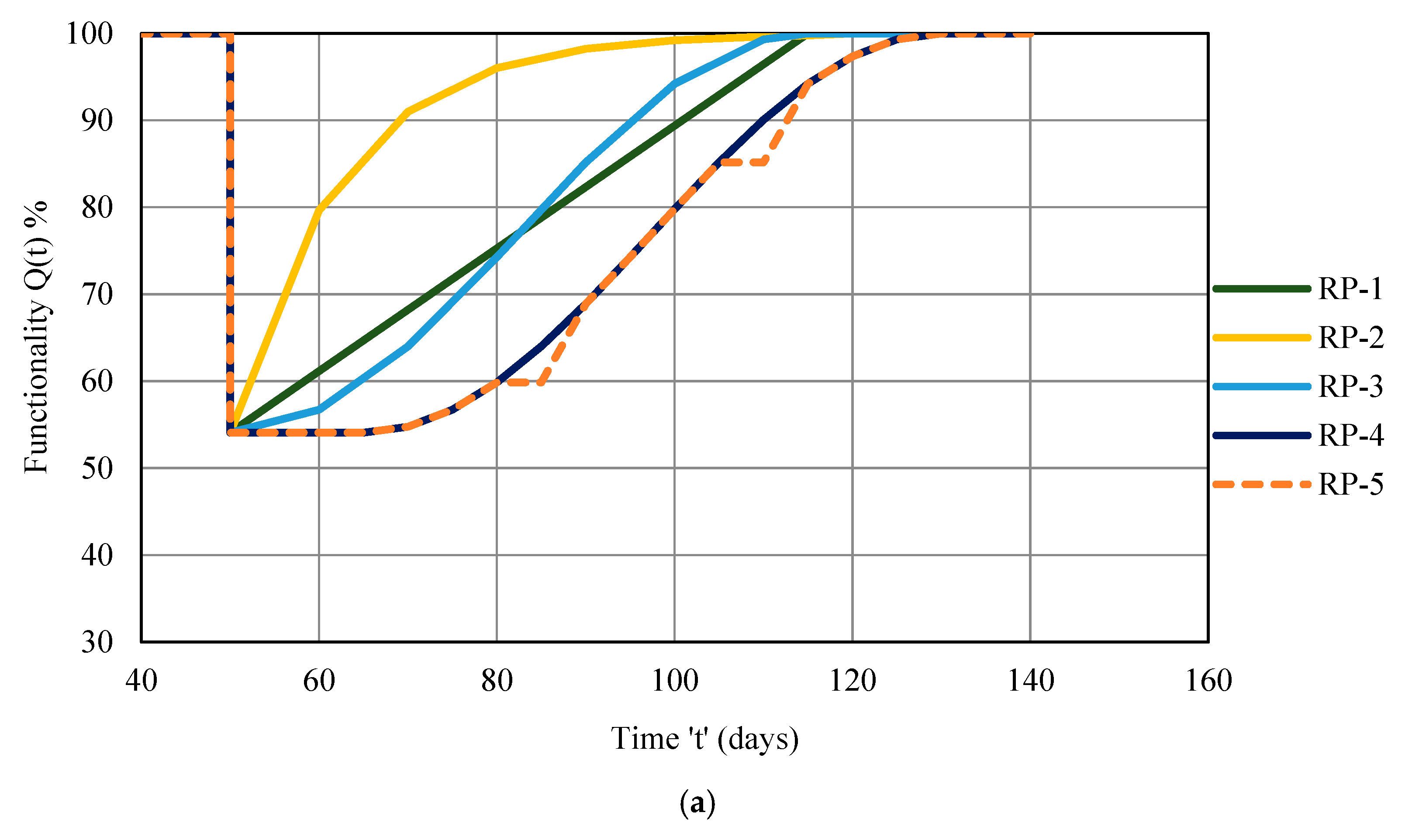
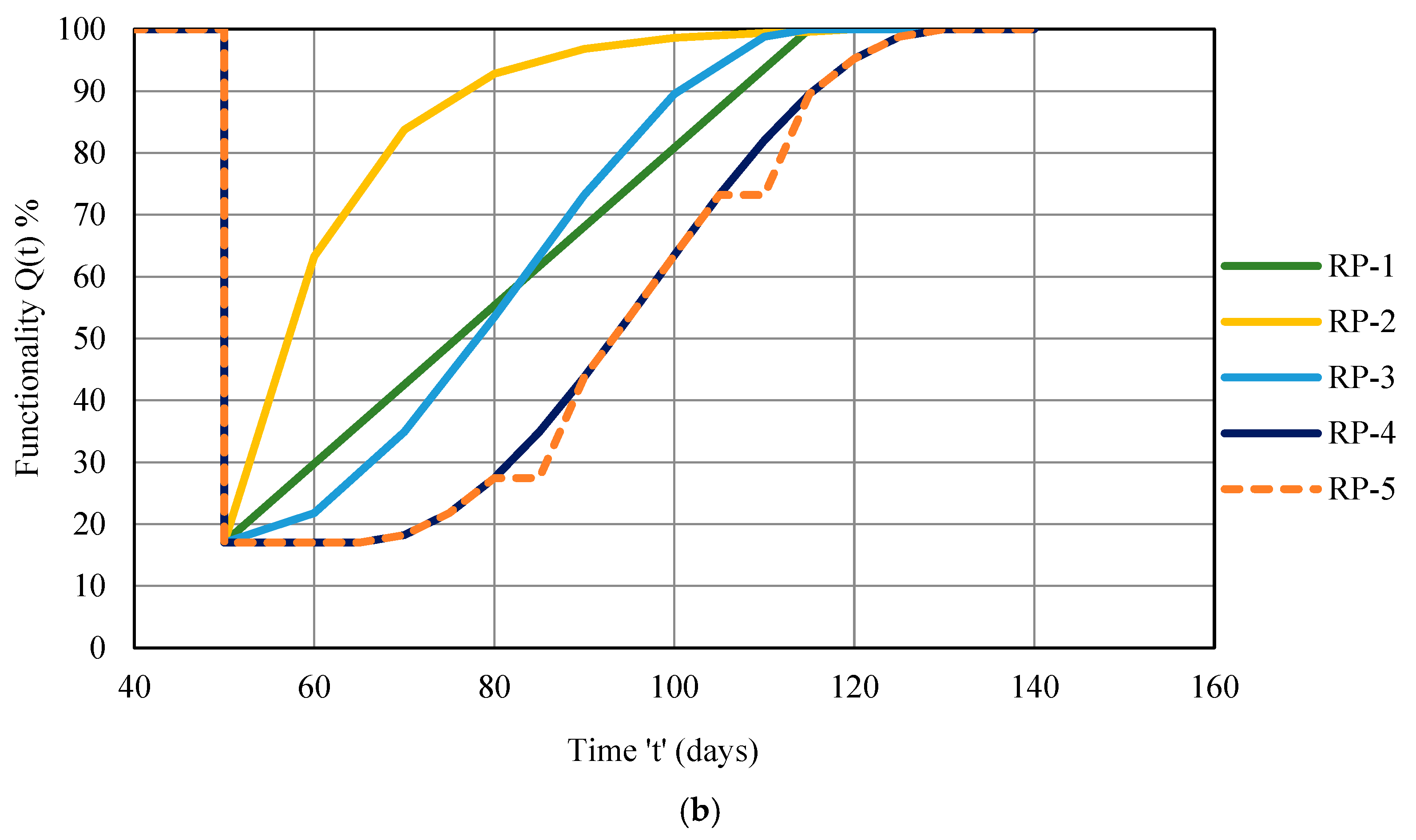
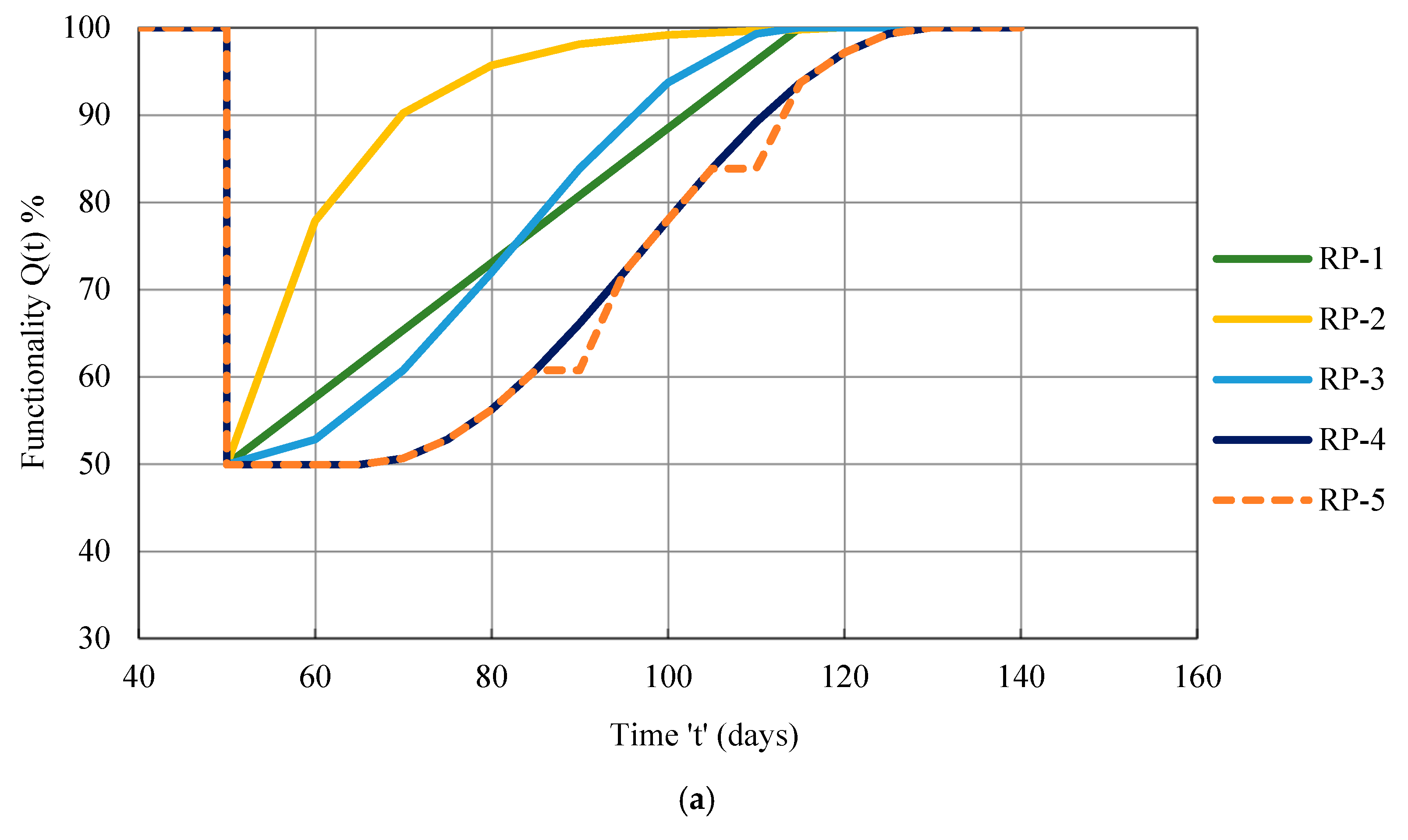
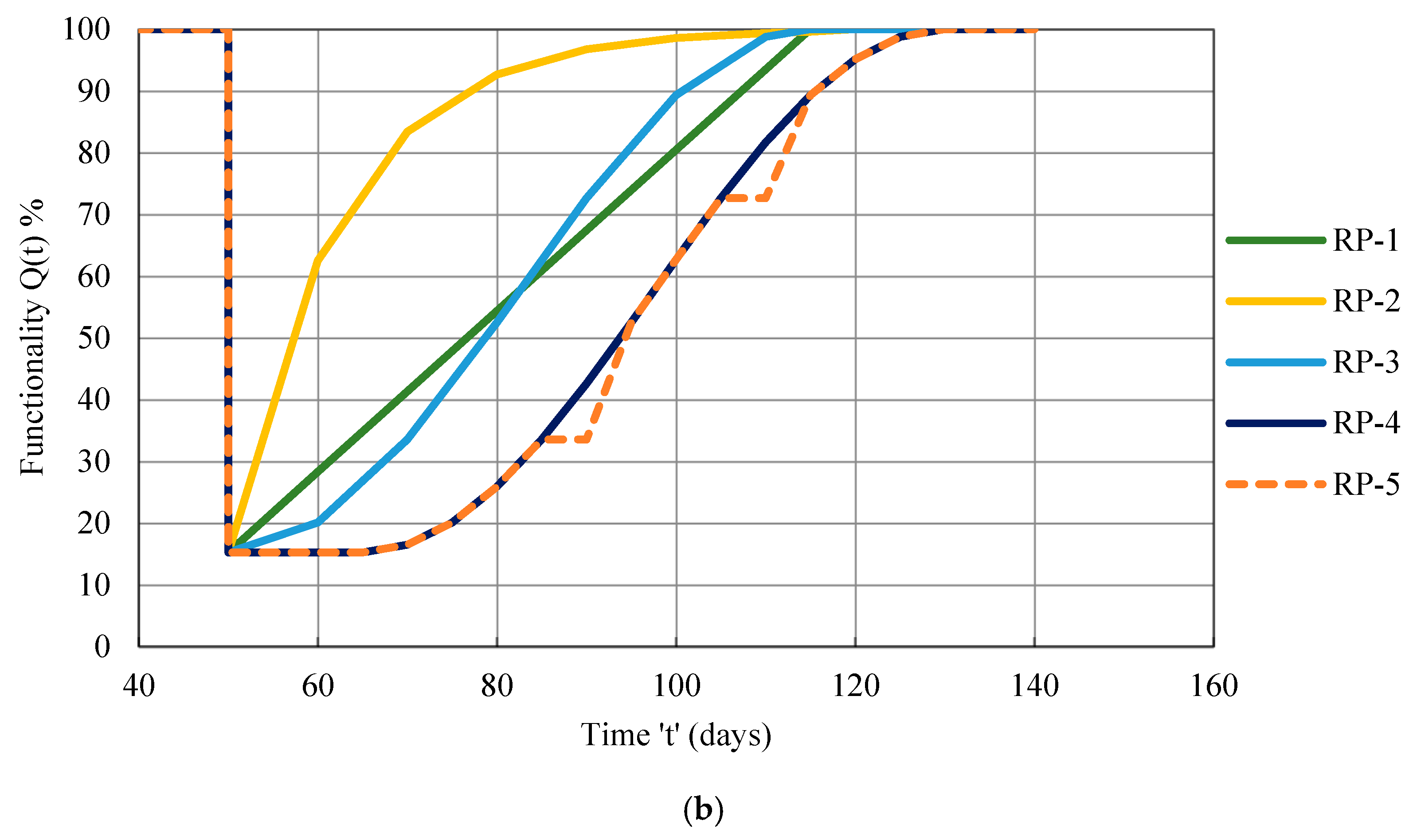
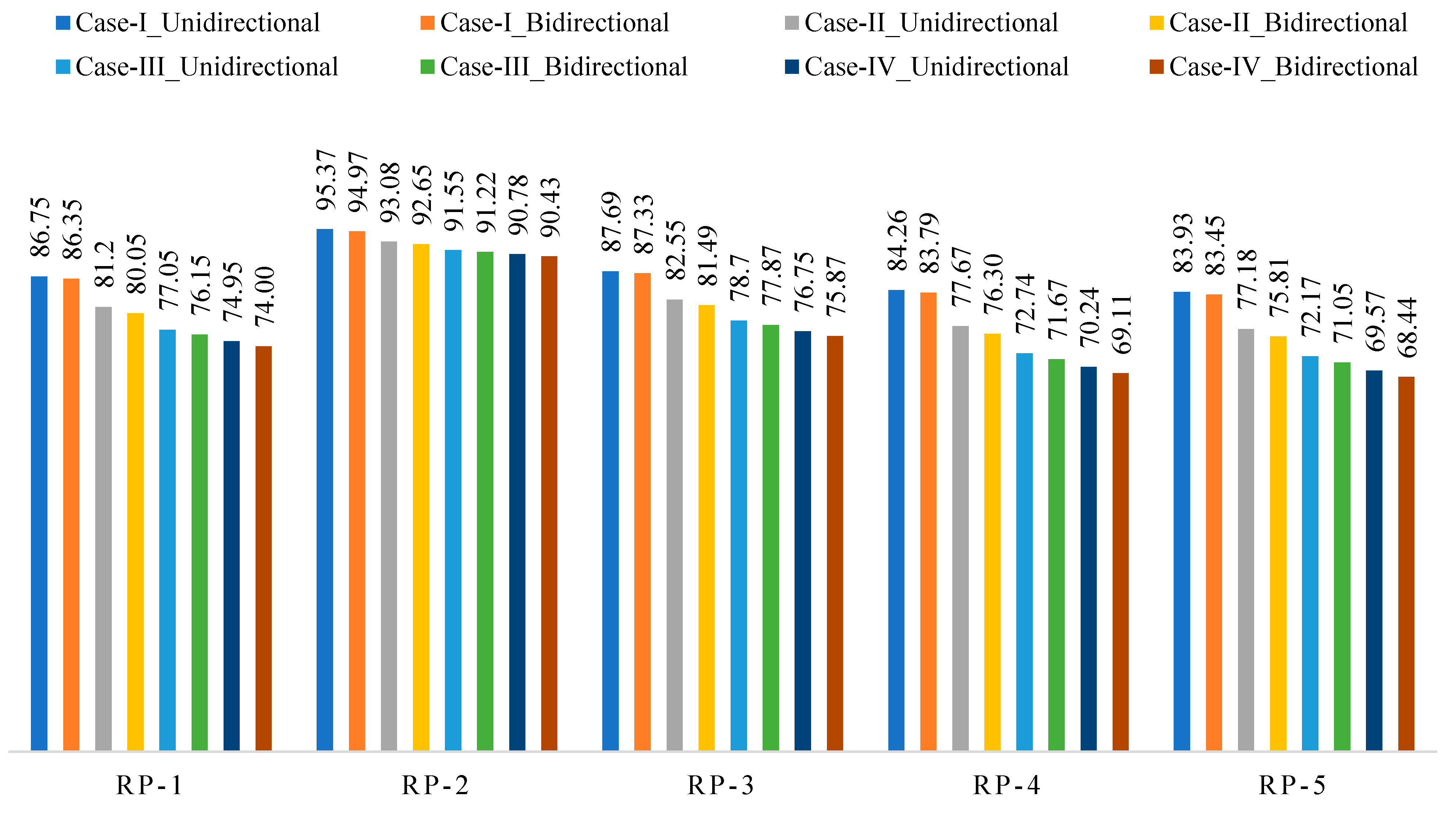
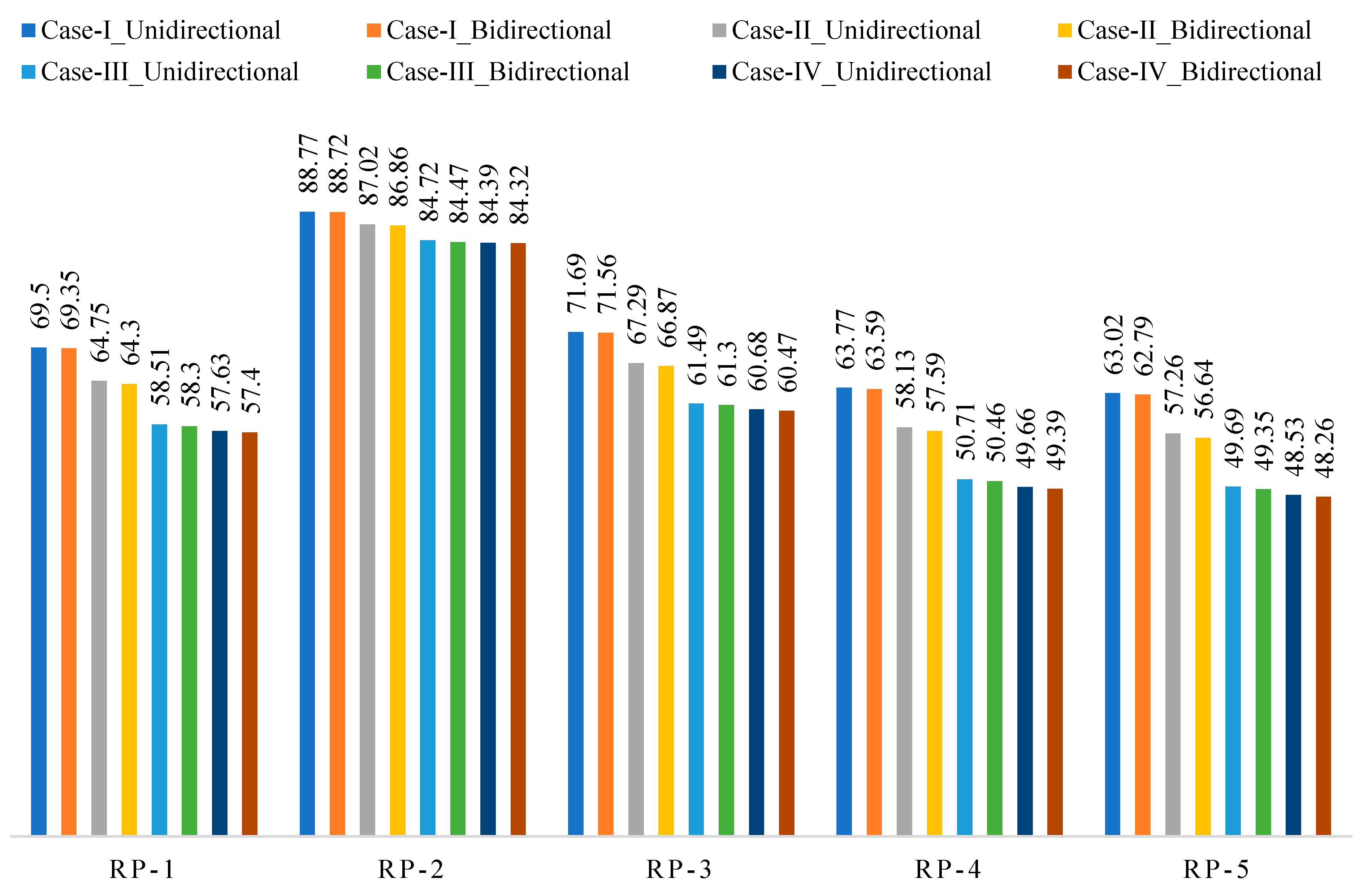
• The five recovery trajectories showed different levels of resilience (RP-1 to RP-5). When compared to other traditional recovery routes, the study’s novel recovery paths (RP-4 and RP-5) provide a slightly higher loss of resilience. This reduction in resilience was due to the inclusion of initial delay and break in the recovery process at RP-4 and RP-5.
• Although the building suffers a large loss in functionality at the MCE level at R = 5 and R = 6, it nevertheless retains over 50% of its resilience under uni-directional and bi-directional loading. This was accomplished by keeping the appropriate ductility demand at R = 6. At bi-directional loading conditions, the larger loss of resilience of around 51.74% was calculated at R equal to 6 building cases. Due to greater damage, recovering this building situation might necessitate higher retrofitting costs. This result demonstrates that the building’s resilience must be taken into account while planning the post-seismic recovery phase, despite other seismic performances.
• From the above results, with consideration of ductility demand, performance level and building’s resilience, the response reduction factor for the building considered in the study has been recommended up to 6 for uni-directional loading, but due to the bi-directional effect, the performable level of the building at higher R factors was affected as it reaches collapse stage. It was concluded from the above results the maximum R factor has been recommended up to 4.
• According to the study’s findings, choosing an appropriate R factor for a building’s design should take into account the structure’s resilience as well as its performance level and ductility requirements.

References

1. ASCE/SEI 7-22; Minimum Design Loads and Associated Criteria for Buildings and Other Structures. American Society of Civil Engineers: Reston, VA, USA, 2005.
2. EN 1998-1; Eurocode 8: Design of Structures for Earthquake Resistance. 1st ed. BSI-Brussels: Brussels, Belgium, 2004.
3. IS: 1893. Part-1; Indian Standard Criteria for Earthquake Resistance Design of Structures. Bureau of Indian Standards: New Delhi, India, 2016.
4. Mondal, A.; Ghosh, S.; Reddy, G.R. Performance-based evaluation of the response reduction factor for ductile RC frames. Eng. Struct. 2018, 56, 1808–1819. [Google Scholar] [CrossRef]
5. Abdollahzadeh, G.; Sadeghi, A. Earthquake recurrence effect on the response reduction factor of steel moment frame. Asian J. Civ. Eng. 2018, 19, 993–1008. [Google Scholar] [CrossRef]
6. Yahmi, D.; Branci, T.; Bouchaïr, A.; Fournely, E. Evaluating the Behaviour Factor of Medium Ductile SMRF Structures. Period. Polytech. Civ. Eng. 2018, 62, 373–385. [Google Scholar] [CrossRef] [Green Version]
7. Tamboli, K.; Amin, J.A. Evaluation of Response Reduction Factor and Ductility Factor of RC Braced Frame. J. Mater. Eng. Struct. 2015, 2, 120–129. [Google Scholar]
8. Nishanth, M.; Visuvasam, J.; Simon, J.; Packiaraj, J.S. Assessment of seismic response reduction factor for moment resisting RC frames. Int. J. IOP Conf. Ser. Mater. Sci. Eng. 2017, 263, 032034. [Google Scholar] [CrossRef]
9. Chaulagain, H.; Rodrigues, H.; Spacone, E.; Guragain, R.; Mallik, R.; Varum, H. Response reduction factor of irregular RC buildings in Kathmandu valley. Earthq. Eng. Eng. Vib. 2014, 13, 455–470. [Google Scholar] [CrossRef]
10. Mohsenian, V.; Mortezaei, A. Evaluation of seismic reliability and multilevel response reduction factor (R factor) for eccentric braced frames with vertical links. Earthq. Struct. 2018, 14, 537–549. [Google Scholar]
11. Patel, K.N.; Amin, J.A. Performance-based assessment of response reduction factor of RC-elevated water tank considering soil flexibility: A case study. Int. J. Adv. Struct. Eng. 2018, 10, 233–247. [Google Scholar] [CrossRef] [Green Version]
12. Jiménez, F.J.P.; Morillas, L. Effect of the Importance Factor on the Seismic Performance of Health Facilities in Medium Seismicity Regions. J. Earthq. Eng. 2022, 26, 546–562. [Google Scholar] [CrossRef]
13. Hussein, M.M.; Gamal, M.; Attia, W.A. Seismic response modification factor for RC-frames with non-uniform dimensions. Cogent Eng. 2021, 8, 1923363. [Google Scholar]
14. Attia, W.A.; Irheem, M.M. Irheem. Boundary condition effect on response modification factor of X-braced steel frames. HBRC J. 2018, 14, 104–121. [Google Scholar] [CrossRef] [Green Version]
15. Keykhosravi, A.; Aghayari, R. Evaluating response modification factor (R) of reinforced concrete frames with chevron brace equipped with steel slit damper. KSCE J. Civ. Eng. 2017, 21, 1417–1423. [Google Scholar] [CrossRef]
16. Kappos, A.J. Evaluation of behaviour factors on the basis of ductility and overstrength studies. Eng. Struct. 1999, 21, 823–835. [Google Scholar] [CrossRef]
17. Patel, B.; Shah, D. Formulation of Response Reduction Factor for RCC Framed Staging of Elevated Water tank using static pushover analysis. In Proceedings of the World Congress on Engineering, London, UK, 30 June–2 July 2010; Volume III. [Google Scholar]
18. Galasso, C.; Maddaloni, G.; Cosenza, E. Uncertainly Analysis of Flexural over strength for Capacity Design of RC Beams. J. Struct. Eng. 2014, 140, 04014037. [Google Scholar] [CrossRef]
19. Abdi, H.; Hejazi, F.; Saifulnaz, R.; Karim, I.A.; Jaafar, M.S. Response modification factor for steel structure equipped with viscous damper device. Int. J. Steel Struct. 2015, 15, 605–622. [Google Scholar] [CrossRef]
20. Prasanth, S.; Ghosh, G. Effect of variation in design acceleration spectrum on the seismic resilience of a building. Asian J. Civ. Eng. 2021, 22, 331–339. [Google Scholar] [CrossRef]
21. Prasanth, S.; Ghosh, G. Effect of cracked section properties on the resilience based seismic performance evaluation of a building. Structures 2021, 34, 1021–1033. [Google Scholar] [CrossRef]
22. Marasco, S.; Cardoni, A.; Noori, A.Z.; Kammouh, O.; Domaneschi, M.; Cimellaro, G.P. Integrated platform to assess seismic resilience at the community level. Sustain. Cities Soc. 2021, 64, 102506. [Google Scholar] [CrossRef]
23. Javad Hashemi, M.; Ali Al-Attraqchi, Y.; Kalfat, R.; Al-Mahaidi, R. Linking seismic resilience into sustainability assessment of limited-ductility R.C. buildings. Eng. Struct. 2019, 188, 121–136. [Google Scholar] [CrossRef]
24. Cimellaro, G.P.; Andrei Reinhorn, M.; Bruneau, M. Framework for analytical quantification of disaster resilience. Eng. Struct. 2010, 32, 3639–3649. [Google Scholar] [CrossRef]
25. Cimellaro, G.P.; Andrei Reinhorn, M.; Bruneau, M. Seismic resilience of a hospital system. Struct. Infrastruct. Eng. 2010, 6, 127–144. [Google Scholar] [CrossRef]
26. Hudson, S.; Cormie, D.; Tufton, E.; Inglis, S. Engineering resilient infrastructure. Proc. Inst. Civ. Eng.-Civ. Eng. 2012, 165, 5–12. [Google Scholar] [CrossRef]
27. Gallagher, D.; Cruickshank, H. Planning under new extremes: Resilience and the most vulnerable. Proc. Inst. Civ. Eng.-Munic. Eng. 2015, 169, 127–137. [Google Scholar] [CrossRef]
28. Grigorian, M.; Kamizi, M. High-performance resilient earthquake-resisting moment frames. Proc. Inst. Civ. Eng.-Struct. Build. 2022, 175, 401–417. [Google Scholar] [CrossRef]
29. Dukes, J.; Mangalathu, S.; Padgett, J.E.; DesRoches, R. Development of a bridge-specific fragility methodology to improve the seismic resilience of bridges. Earthq. Struct. 2018, 15, 253–261. [Google Scholar]
30. Haselton, C.B.; Deierlein, G.G. Assessing Seismic Collapse Safety of Modern Reinforced Concrete Moment-Frame Buildings; PEER report 2007/08; Pacific Engineering Research Center, University of California: Berkeley, CA, USA, 2008. [Google Scholar]
31. Haselton, C.B.; Liel, A.B.; Deierlein, G.G.; Dean, B.S.; Chou, J.H. Seismic collapse safety of reinforced concrete buildings—I: Assessment of ductile moment frames. J. Struct. Eng. 2011, 137, 481–491. [Google Scholar] [CrossRef] [Green Version]
32. Liel, A.B.; Haselton, C.B.; Deierlein, G.G. Seismic collapse safety of reinforced concrete buildings. II: Comparative assessment of nonductile and ductile moment frames. J. Struct. Eng. 2011, 137, 492–502. [Google Scholar] [CrossRef]
33. Computers and Structures. Inc. SAP V22. In Integrated Software for Structural Analysis and Design; Computers and Structures. Inc.: Berkley, CA, USA, 2000. [Google Scholar]
34. Izzuddin, B.A.; Karayannis, C.G.; Elnashai, A.S. Advanced nonlinear formulation for reinforced concrete beam-columns. J. Struct. Eng. 1994, 120, 2913–2934. [Google Scholar] [CrossRef]
35. Ali Hadigheh, S.; Saeed Mahini, S.; Setunge, S.; Stephen Mahin, A. A preliminary case study of resilience and performance of rehabilitated buildings subjected to earthquakes. Earthq. Struct. 2016, 11, 967–982. [Google Scholar] [CrossRef]
36. Gupta, P.K.; Ghosh, G. Effect of Bi-directional excitation on a curved bridge with lead rubber bearing. Mater. Today Proc. 2021, 44, 2239–2244. [Google Scholar] [CrossRef]
37. Gupta, P.K.; Ghosh, G.; Pandey, D.K. Parametric study of effects of vertical ground motions on base isolated structures. J. Earthq. Eng. 2021, 25, 434–454. [Google Scholar] [CrossRef]
38. Gupta, P.K.; Ghosh, G.; Kumar, V.; Paramasivam, P.; Dhanasekaran, S. Effectiveness of LRB in Curved Bridge Isolation: A Numerical Study. Appl. Sci. 2022, 12, 11289. [Google Scholar] [CrossRef]
39. ATC-40; Seismic Evaluation and Retrofit of Reinforced Concrete Buildings. Applied Technology Council: Redwood City, CA, USA, 1996.
40. Gupta, P.K.; Ghosh, G. Effect of various aspects on the seismic performance of a curved bridge with HDR bearings. Earthq. Struct. 2020, 19, 427–444. [Google Scholar]
41. ASCE/SEI 41-17; Seismic Evaluation and Retrofit of Existing Buildings. American Society of Civil Engineers: Reston, VA, USA, 2017.
42. FEMA-440; Improvement of Nonlinear Static Seismic Analysis Procedures. Federal Emergency Management Agency: Washington, DC, USA, 2005.
43. Department of Homeland Society. HAZUS-MR4 Technical Manual. In Multihazard Loss Estimation Methodology; Department of Homeland Society: Washington, DC, USA, 2003. [Google Scholar]
44. Kumar, A.; Sharma, K.; Dixit, A.R. A review on the mechanical properties of polymer composites reinforced by carbon nanotubes and graphene. Carbon Lett. 2021, 31, 149–165. [Google Scholar] [CrossRef]
45. Bruneau, M.; Chang, S.E.; Eguchi, R.T.; Lee, G.C.; O’Rourke, T.D.; Reinhorn, A.M.; Shinozuka, M.; Tierney, K.; Wallace, W.A.; Von Winterfeldt, D. A framework to quantitatively assess and enhance the seismic resilience of communities. Earthq. Spectra 2003, 19, 733–752. [Google Scholar] [CrossRef] [Green Version]
46. Prasanth, S.; Ghosh, G.; Gupta, P.K.; Casapulla, C.; Giresini, L. Accounting for Resilience in the Selection of R Factors for a RC Unsymmetrical Building. Appl. Sci. 2023, 13, 1316. [Google Scholar] [CrossRef]
47. Kumar, A.; Ghosh, G.; Gupta, P.K.; Kumar, V.; Paramasivam, P. Seismic hazard analysis of Silchar city located in North East India. Geomat. Nat. Hazards Risk 2023, 14, 2170831. [Google Scholar] [CrossRef]
Figure 1. View of symmetrical building (a) Plan wise (b) Elevation wise.
Buildings 13 00626 g001
Figure 2. Three-dimensional view of the symmetrical building.
Buildings 13 00626 g002
Figure 3. El Centro ground motion.
Buildings 13 00626 g003
Figure 4. Bam ground motion.
Buildings 13 00626 g004
Figure 5. Kobe ground motion.
Buildings 13 00626 g005
Figure 6. San Fernando ground motion.
Buildings 13 00626 g006
Figure 7. Tabas ground motion.
Buildings 13 00626 g007
Figure 8. Matched response spectrum.
Buildings 13 00626 g008
Figure 9. Schematic representation of inelastic design.
Buildings 13 00626 g009
Figure 10. Schematic representation on recovery of a building with respect to R factor.
Buildings 13 00626 g010
Figure 11. Displacement envelope at DBE design level at lower R factor (R = 3).
Buildings 13 00626 g011
Figure 12. Displacement envelope at DBE design level at higher R factor (R = 6).
Buildings 13 00626 g012
Figure 13. Displacement envelope at MCE design level at lower R factor (R = 3).
Buildings 13 00626 g013
Figure 14. Displacement envelope at MCE design level at higher R factor (R = 6).
Buildings 13 00626 g014
Figure 15. Generalized Force-deformation curve [34].
Buildings 13 00626 g015
Figure 16. Schematic representation of performance level of each building case at MCE design level under uni-directional loading.
Buildings 13 00626 g016
Figure 17. Schematic representation of performance level of each building case at MCE design level under bi-directional loading.
Buildings 13 00626 g017
Figure 18. Fragility curve for symmetrical building case-I (R = 3).
Buildings 13 00626 g018
Figure 19. Fragility curve for symmetrical building case-II (R = 4).
Buildings 13 00626 g019
Figure 20. Fragility curve for symmetrical building case-III (R = 5).
Buildings 13 00626 g020
Figure 21. Fragility curve for symmetrical building case-IV (R = 6).
Buildings 13 00626 g021
Figure 22. Different types of recovery paths (RP-1 to RP-5).
Buildings 13 00626 g022
Figure 23. (a,b). Functionality curves of the building corresponding to case-I. (a) At DBE design level. (b) At MCE design level.
Buildings 13 00626 g023aBuildings 13 00626 g023b
Figure 24. (a,b). Functionality curves of the building corresponding to case-II. (a) At DBE design level. (b) At MCE design level.
Buildings 13 00626 g024aBuildings 13 00626 g024b
Figure 25. (a,b). Functionality curves of the building corresponding to case-III. (a) At DBE design level. (b) At MCE design level.
Buildings 13 00626 g025aBuildings 13 00626 g025b
Figure 26. (a,b). Functionality curves of the building corresponding to case-IV. (a) At DBE design level. (b) At MCE design level.
Buildings 13 00626 g026aBuildings 13 00626 g026b
Figure 27. Comparison of symmetrical building’s resilience under uni- and bi-directional loading at DBE design level.
Buildings 13 00626 g027
Figure 28. Comparison of symmetrical building’s resilience under uni and bi-directional loading at MCE design level.
Buildings 13 00626 g028