Synthetic Datasets for Rebar Instance Segmentation Using Mask R-CNN

Abstract

The construction and inspection of reinforcement rebar currently rely entirely on manual work, which leads to problems such as high labor requirements and labor costs. Rebar image detection using deep learning algorithms can be employed in construction quality inspection and intelligent construction; it can check the number, spacing, and diameter of rebar on a construction site, and guide robots to complete rebar tying. However, the application of deep learning algorithms relies on a large number of datasets to train models, while manual data collection and annotation are time-consuming and laborious. In contrast, using synthetic datasets can achieve a high degree of automation of annotation. In this study, using rebar as an example, we proposed a mask annotation methodology based on BIM software and rendering software, which can establish a large and diverse training set for instance segmentation, without manual labeling. The Mask R-CNN trained using both real and synthetic datasets demonstrated a better performance than the models trained using only real datasets or synthetic datasets. This synthetic dataset generation method could be widely used for various image segmentation tasks and provides a reference for other computer vision engineering tasks and deep learning tasks in related fields.

1. Introduction

Rebar tying work is a highly labor-intensive job with an unfavorable working environment and may cause musculoskeletal disorders in rebar workers [1]. Therefore, the use of robots to achieve automatic rebar tying is a necessary direction of development for on-site construction operations. To use robots for automatic rebar tying, it is necessary to identify the crosspoints and then carry out path planning to complete the rebar tying work [2].

The quality inspection of reinforcement construction at a large scale is also a problem. Thousands of reinforcement bars are inspected manually to see if their quantity and spacing meet the design parameters, and this workload is extremely difficult to manage. Therefore, at present, construction sites are inspected randomly to check the quality of rebar, but there is still the problem of inspection errors and omissions.

Therefore, the photographic acquisition of on-site rebar and rebar instance segmentation could be carried out using deep learning algorithms, to quickly and accurately determine the location and quantity of rebar; this can provide data support for the automatic tying of rebar and realize the quality inspection of rebar construction at a large scale. The application of computer visual technology for rebar detection on construction sites will help to achieve a reduction in construction costs and labor expenses, which are of primary concern to customers. Based on the concept and methodology of customer relationship management, this will greatly benefit projects [3].

A series of computer vision-based automated rebar detection methods have been proposed by researchers, all of which can identify the spacing or diameter of rebar. These include vision methods based on laser rangefinders and corner detection [4], point cloud data processing methods based on machine learning [5], and image segmentation methods based on deep learning [6]. However, the traditional image processing method used in [4] made it difficult to deal with complex environments. The authors of [5] had to use laser scanners to scan multiple stations, which incurred high equipment costs and was tedious. In [6], although rebar counting and diameter estimation were achieved using a convolutional neural network segmentation algorithm combined with homography, this method was difficult to apply to the spacing and diameter detection of rebar in the rebar mesh.

The application of deep learning algorithms in a specific field is often limited by the size and quality of the dataset and its annotations [7]. The instance segmentation of rebar requires a large number of annotated training set images, where each rebar in each image needs to be annotated. At present, annotation is mainly carried out manually, making it time-consuming and laborious, and resulting in a low annotation accuracy. Using cell phones, cameras, drones, and other devices to shoot and collect data also has the disadvantages of consuming more time, requiring pre-planning and coordination, and having fewer or more-scattered target objects. Due to the large variety and weight of steel rebar, it is difficult to collect and label datasets manually.

The efficient building of high-quality datasets has become key to the successful application of deep learning techniques in the engineering field. Therefore, using 3D software to generate realistic images and implement automatic annotation has become a solution to the problem of dataset acquisition. Mohamed H. Elnabawi et al. [8] implemented a synthetic urban local specific weather dataset for the estimation of energy demand. However, this is not a suitable method for creating synthetic image datasets. Boyong He et al. [9] used Unity3D to create a synthetic ship image dataset for ship object detection. NVIDIA and Unity have released synthetic dataset generation plugins based on the Unreal Engine (UE) and Unity3D, respectively [10,11]. The authors of [9,10,11] imported 3D models into Unreal Engine and Unity3D to render realistic pictures and construct datasets. However, Unreal Engine and Unity3D are complicated and require a certain programming process, which entails a high learning cost. It is difficult to promote synthetic dataset generation methods based on these software packages. Zhiyong Zhang et al. [12] proposed a methodology for creating synthetic data for sand-like granular instance segmentation. However, this method simply overlaps the images of the target objects, ignoring the three-dimensional relationship and light and shadow effects, which is not sufficiently realistic. Yeji Hong et al. [13] used building information models to create BIM images and labels, then used generative adversarial networks (GANs) to perform translation of the BIM images into photographs, to achieve the creation of synthetic infrastructure scene datasets.

The previous methods of synthetic image data creation and automatic annotation involving Unity3D, UE, or GANs are not concise enough. In order to efficiently create synthetic datasets suitable for image segmentation tasks, this paper takes the instance segmentation task of rebar as an example and proposes a simple and fast method of creating instance segmentation datasets. The method includes BIM modeling and using rendering software to output realistic images and corresponding annotations. Finally, we compared the performance of a real dataset and a synthetic dataset in network prediction, and verified the rationality and effectiveness of using synthetic data for network training.

The method proposed in this paper can be used to easily and quickly create synthetic rebar instance segmentation datasets for the training of rebar recognition algorithm models. The proposed method has good generality and can be used to create semantic segmentation or instance segmentation synthesis datasets for any type of target object and thus provides a good technical solution for the rapid acquisition of training sets for visual recognition tasks in engineering.

2. Process and Methodology

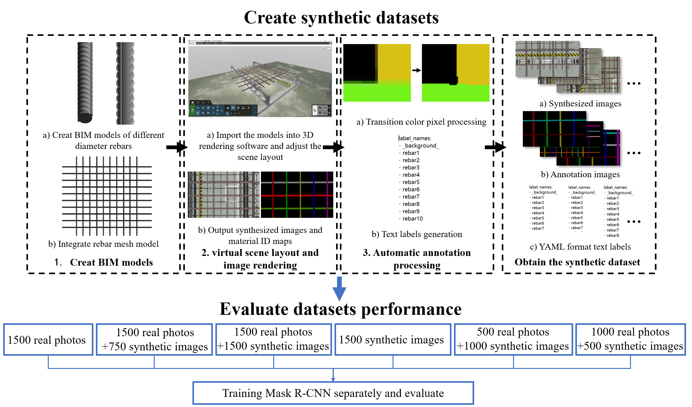
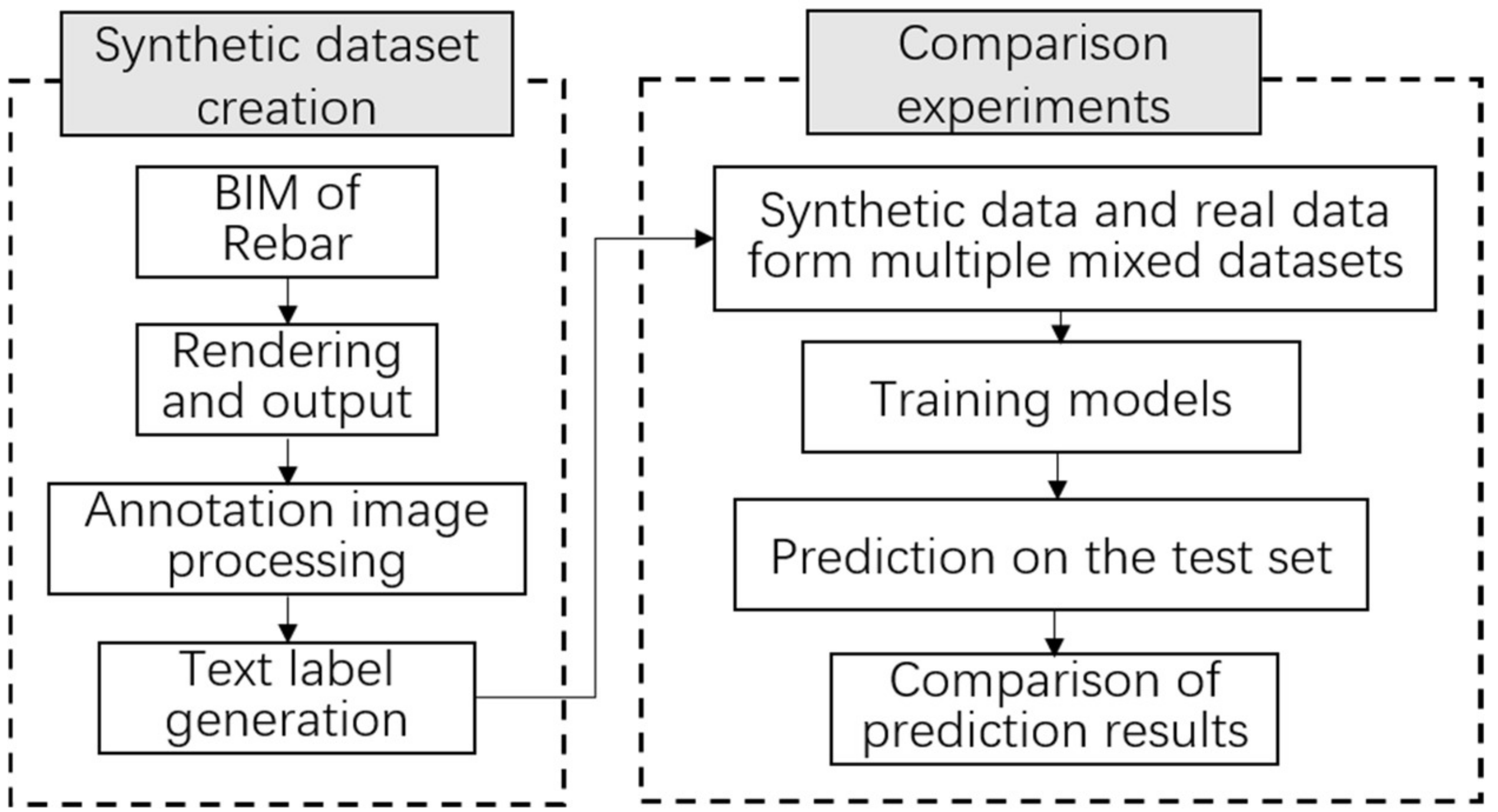
The processes for making a synthetic image dataset for rebar and comparing the performance of the datasets are shown in Figure 1.

In the synthetic dataset creation process, creating the rebar BIM was the first step. Revit software was used for modeling. The second step was to import the rebar model into the 3D rendering software, adjust the material, arrange the scene, and render the picture and its corresponding material ID map image. The third step was to use the program to process the material ID map image to make it an annotation image that could be used to train the Mask R-CNN network. The fourth step was to generate the text labels required for network training based on the annotation image in the previous step. Finally, the synthetic dataset consisted of three parts: the rendered synthetic images, the annotation images of the synthetic images, and the YAML-format text labels corresponding to the annotation images.

After the creation of the synthetic dataset was completed, the synthetic images were mixed with the real rebar mesh images in different numbers, to build six training sets, and a Mask R-CNN network was used for benchmark testing, to compare the performance of the models trained in each training set and to illustrate the effectiveness and rationality of using synthetic images as a training set.

3. Synthetic Image Creation Method

3.1. BIM and Virtual Scene Layout

In this step, we created a rebar model in Revit and imported it into the 3D rendering software. Then, we adjusted the scene layout in the rendering software as accurately as possible, so that the rendered output was as similar as possible to the real photograph.

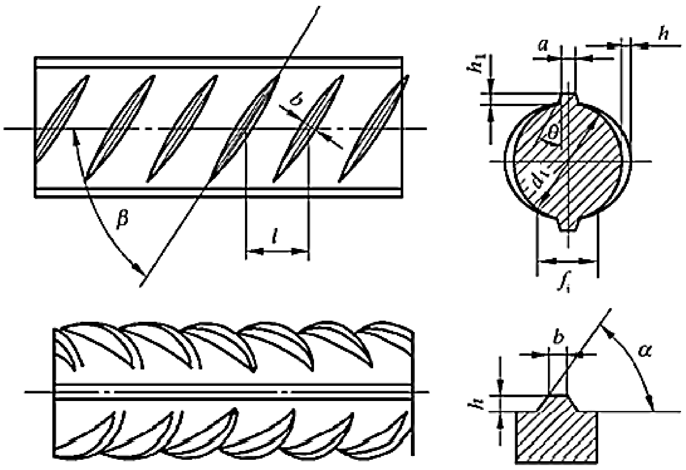
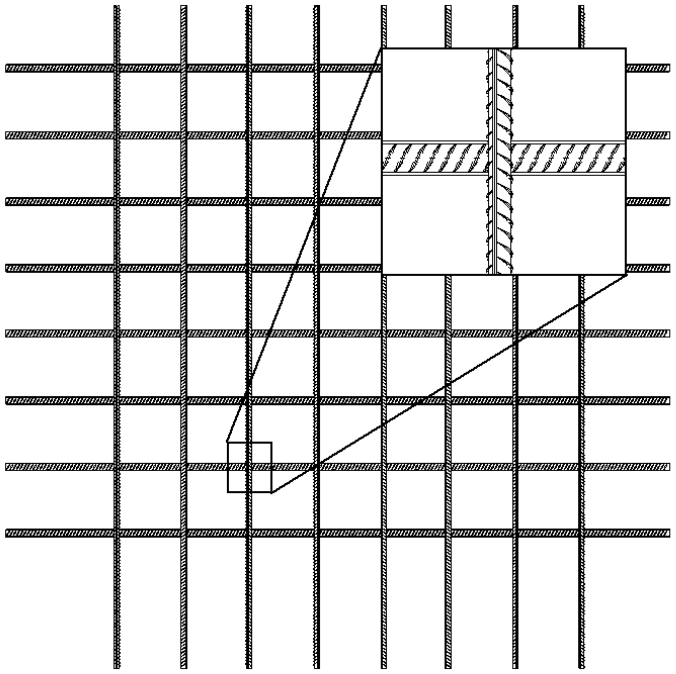
Using Revit, parametric modeling was performed on rebar with common diameters. Relevant specifications were established to create detailed regulations on the geometric shape of rebar (Figure 2). Specific values are given for the inner diameter, the height of transverse ribs, the height of longitudinal ribs, the width of transverse ribs, the width of longitudinal ribs, the thread spacing, and the maximum distance between the ends of the transverse ribs of the pieces of rebar of each diameter. Value ranges are given for the oblique angles of the transverse ribs and the oblique angles of the longitudinal ribs. In this paper, three sizes of rebar, with nominal diameters of 16, 20, and 25 mm, were selected for modeling. After referring to the actual rebar geometry, the angle between the transverse rib and the longitudinal axis of the rebar model was set to 60°, and the oblique angle of the longitudinal rib was set to 10°. After completing the modeling of these three kinds of rebar with different diameters, the three models were used to build four different rebar mesh models, to enrich the information in the synthetic dataset. The specific layout is shown in

Table 1. Parameters of the rebar mesh model.

Mesh Model No.	Transverse Model Diameter (Number)	Longitudinal Model Diameter (Number)	Spacing (mm)
1	φ20 (10)	φ20 (10)	150
2	φ20 (10)	φ16 (10)	150
3	φ20 (8)	φ25 (8)	200
4	φ20 (8)	φ16 (8)	200

, and the rebar mesh model is shown in Figure 3.

The meanings of the symbols in Figure 2 are as follows:

$d_1$—the inner diameter; $\alpha$—the oblique angles of the transverse ribs; $h$—the height of the transverse ribs; $\beta$—the angle between the transverse rib and the longitudinal axis; $h_1$—the height of the longitudinal ribs; $\theta$—the oblique angles of the longitudinal ribs; $a$—the longitudinal rib top width; $l$—the transverse rib spacing; $b$—the transverse rib top width; $f_i$—the distance between ends of the transverse ribs.

In order to increase the amount of data and increase the realism of the final synthesized picture, each rebar in the mesh model can be randomly rotated around the longitudinal axis by a certain angle.

The values of the rebar’s geometric parameters in the specification were accurate to 0.1 mm, but Revit cannot draw a line with a length less than 0.8 mm, which would lead to inaccurate modeling. Therefore, when modeling, all dimensions were uniformly enlarged 10 times. Then, the model could be reduced to the original size in the rendering software. Additionally, the size of the rebar mesh model could not be changed in the rendering software, but other models used for the scene layout could be enlarged to a suitable size.

After the rebar model was completed, it was imported into the rendering software for virtual scene layout. The purpose of this was to make the synthetic picture look as similar as possible to the real photograph, so as to contain more complex information. The scene layout was adjusted according to the actual scene, to make it as similar as possible.

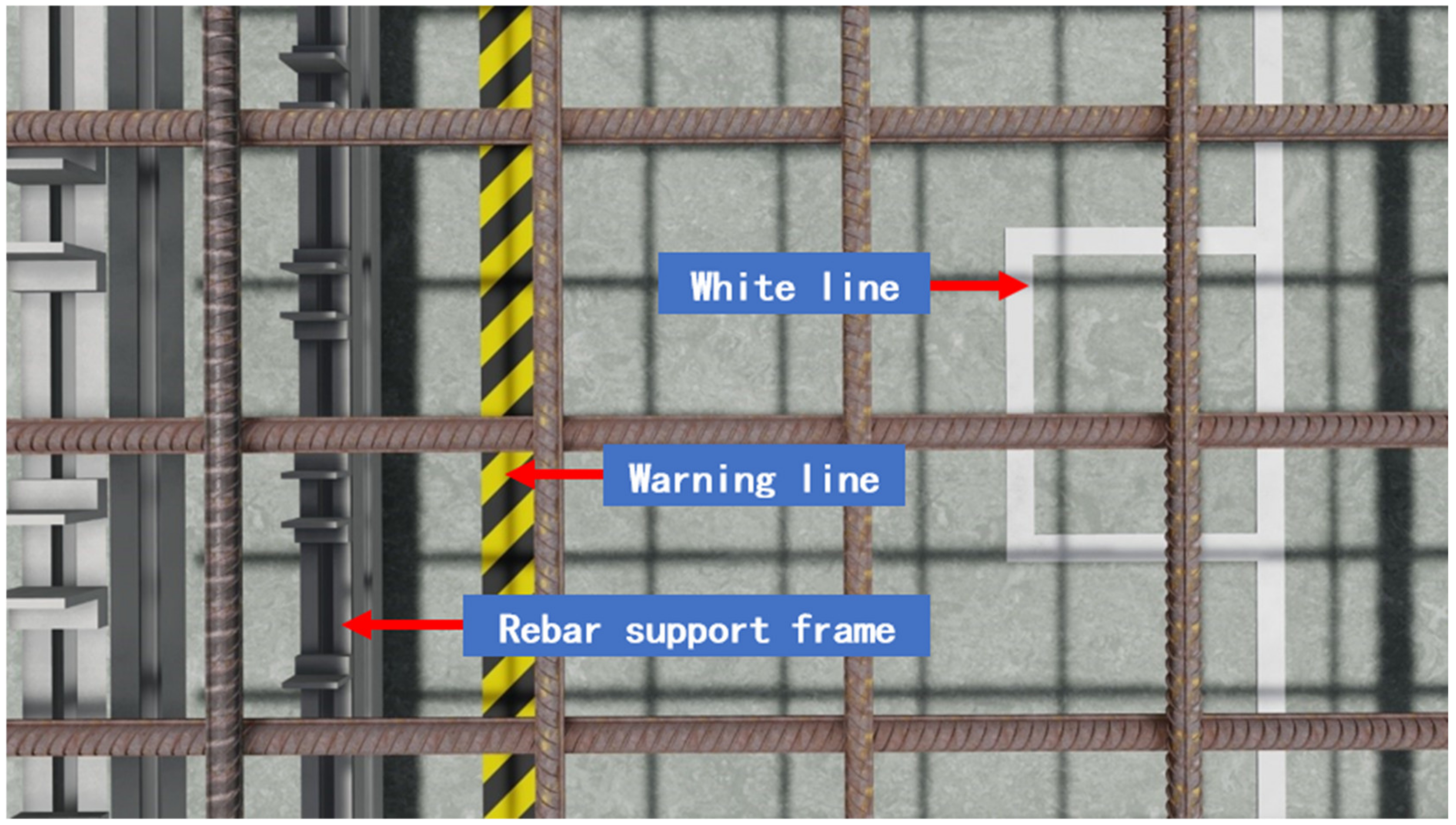
To describe the image rendering steps, let us take the Lumion 11 software as an example. First, create a blank scene, import the rebar mesh model into the scene, and adjust it to the appropriate position and size. In order to make the scene of the rendered picture as similar as possible to the real picture, a ground similar to that in the real picture is set in the virtual scene. Figure 4 shows a specific synthetic scene layout that is similar to our laboratory scene. To capture the context of the laboratory, it is appropriate to adjust the synthetic scene to appear similar to the real scene. There are white lines and yellow-black warning line on the ground. The bottom frame of the rebar support frame, made of aluminum alloy, is also placed. These are all elements that exist in the real scene.

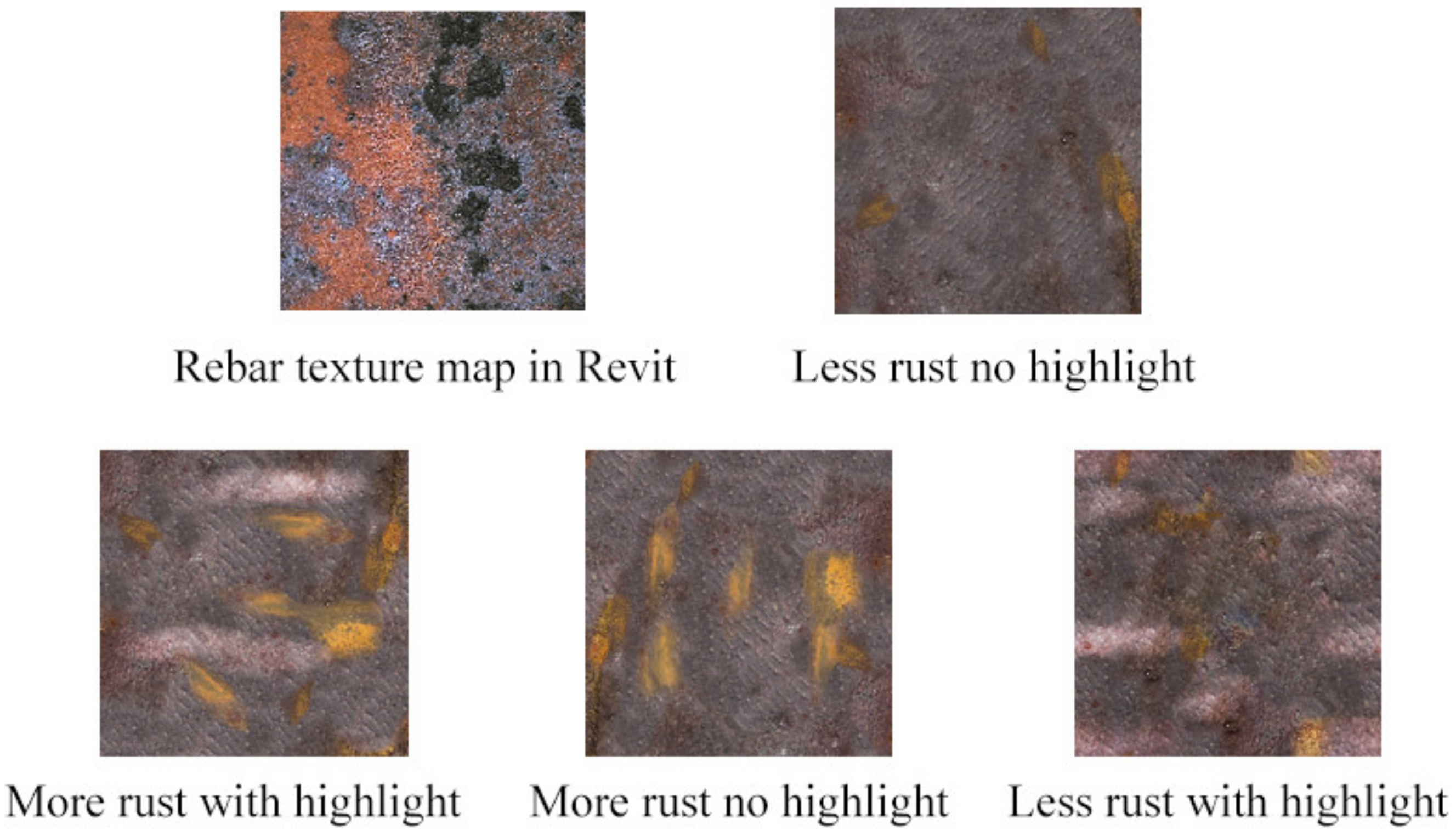
In order to ensure the authenticity and diversity of the synthesized data, for rebar material mapping, we used a built-in rebar map made in Revit and four maps made from real rebar photographs (Figure 5), which were randomly assigned to each rebar. In Figure 5, except the first texture map from Revit, all of the maps were clipped from different real rebar photographs and edited in image processing software. In the image processing software, we adjusted the proportion of the rust pattern and the highlight pattern to ensure the diversity of the texture map.

3.2. Image Rendering

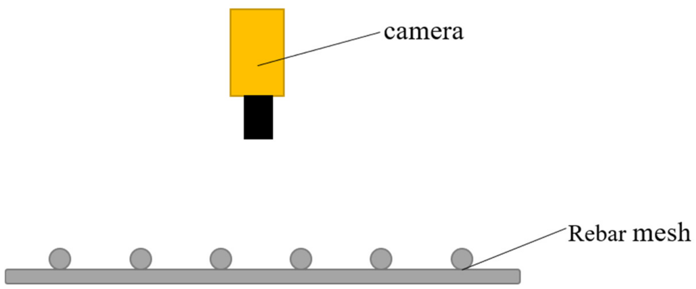
The rendering method of the synthesized image is shown in Figure 6 and works as follows: First, point the camera lens vertically downward, so that the optical axis is perpendicular to the plane of the rebar mesh; ensure that the edge of the image is parallel with or perpendicular to the longitudinal axis of the rebar, and that the number of rebar pieces in the field of view is appropriate (about 10). Then, make translation animations in six directions (front, back, left, right, up, and down), and finally output a jpg-format image in the form of an image frame sequence, to obtain the composite images. The rendering speed should be about 1 s per image. The specific speed should be related to the hardware configuration. The highest rendering quality should be selected here, and the output resolution should be 1280 × 720 pixels. In order to make the picture similar to that seen by the human eye, adjust the focal length to 24 mm, and filters or special effects that cause distortion should not be used. To increase data complexity, image attributes such as shadows, light color temperature, and brightness can be appropriately adjusted.

The lens settings when rendering should be adjusted according to the actual situation. The above lens movement mode was only set for the rebar recognition test in this article.

3.3. Automatic Annotation

After the scene layout arrangement, use the animation recording function in Lumion to render the synthetic images, and the material ID map images are used as labels to realize automatic labeling.

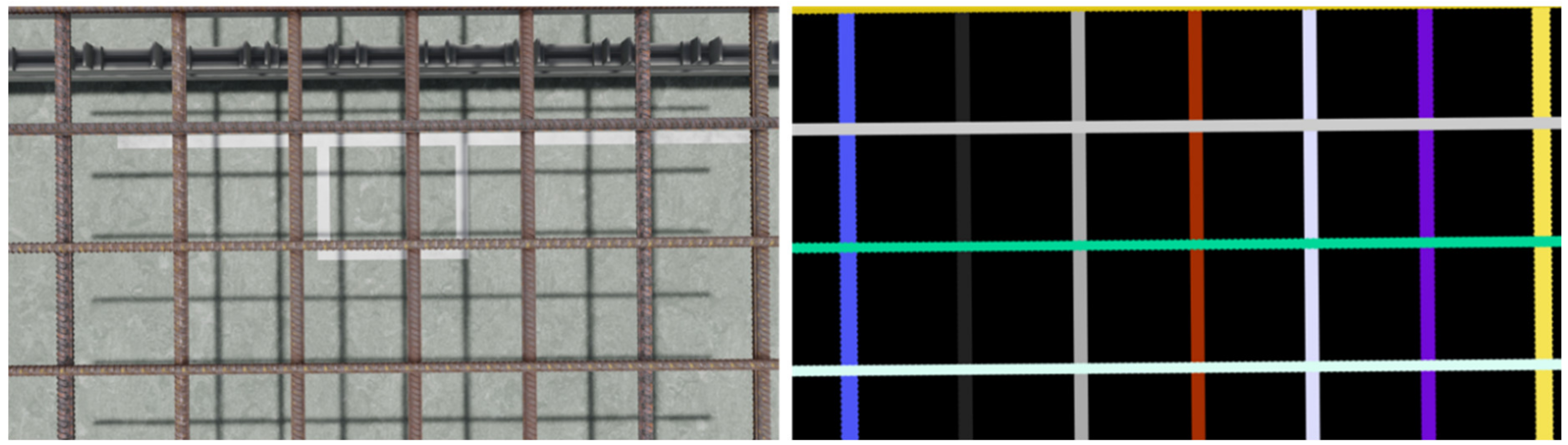
In the instance segmentation label images of the rebar, each instance should be covered by a different color mask, and the background should remain black. Since each rebar has been previously set to a different material in Revit, each rebar will be identified by a solid area of a different color on the material ID map. At this time, if models other than that of the rebar are hidden, the background pixels can be guaranteed to be all black, as shown in Figure 7.

Since the corresponding color of each material in the material ID map rendered by Lumion cannot be specified manually, the system may set the color of a certain material in the ID map to black when there are many types of material in the scene, causing it to have the same material ID color as the background. When this happens, it is necessary to hide the model corresponding to this material, and then render and output the image and material ID map.

When exporting the material ID map, first, copy the footage used for rendering the synthetic image, set all models except the target object to another layer in edit mode, and hide this layer (only the rebar model should be kept here; hide the rest of the models). Then, use the same footage settings as in the previous step when exporting the synthetic image. Check the “M” button in the additional output settings, output the png-format image, and obtain the material ID map corresponding to each image. As the output material ID map will be suffixed onto the file name, use the program for batch renaming, so that the name is exactly the same as that of the corresponding synthetic image file, except for the file type suffix. If using other 3D software to render the picture, you can find a way to output the material ID map or manually set each rebar to a different-colored material and output it again using the same footage.

The training set of Mask R-CNN includes three parts: RGB images, annotation images, and text labels. The text labels are in yaml format. In a yaml file, the first line is “label_names:”, the second line is “- _background_”, and the third line is “- rebar1”, and the subsequent lines are “- rebar2”, “- rebar3”, etc. The specific number of lines is determined by the number of rebar pieces in the image. Thus far, we have obtained the synthetic pictures, the corresponding annotation images, and the text labels, and placed them into folders named “imgs”, “mask”, and “yaml”, respectively, to complete the creation of the rebar synthetic dataset.

This article used the four rebar mesh models in Table 1, with different backgrounds, material maps, lighting settings, and camera path animations, and rendered a total of 2500 virtual synthetic pictures of rebar mesh and their material ID maps. The material ID map is the preliminary result of automatic labeling.

The following is the rebar synthetic dataset download path: https://github.com/whiesty/synthetic-datasets-for-rebar/releases/download/file/synthetic.dataset.for.rebar.zip (accessed on 13 February 2023).

3.4. Transition Color Processing of Annotation Image

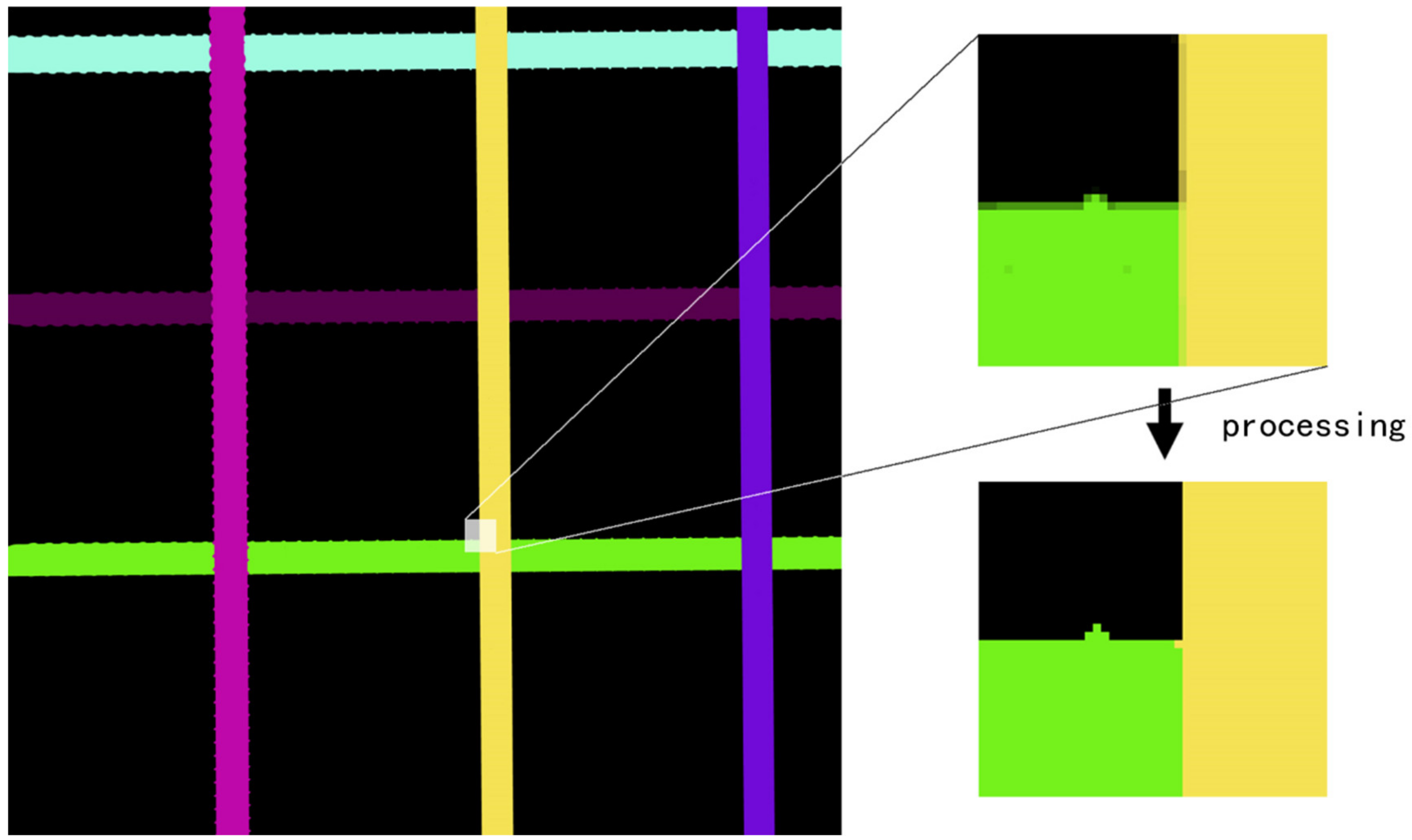
Since the material ID map output by Lumion has a transition color at the edge of the mask (Figure 8), it must be processed by the program before it can be input into the Mask R-CNN network as an annotation image. As each color in the annotation image should correspond to an instance target object, if the transition color already exists, the network will mistakenly read it as an annotation of other instances.

Therefore, this section proposes an image processing method for the transition color in the material ID map output by Lumion, programmed to achieve the following functions: (1) change the transition color in the material ID map to the correct annotation color; (2) save the annotation image as a P-mode single-channel png format image with the palette.

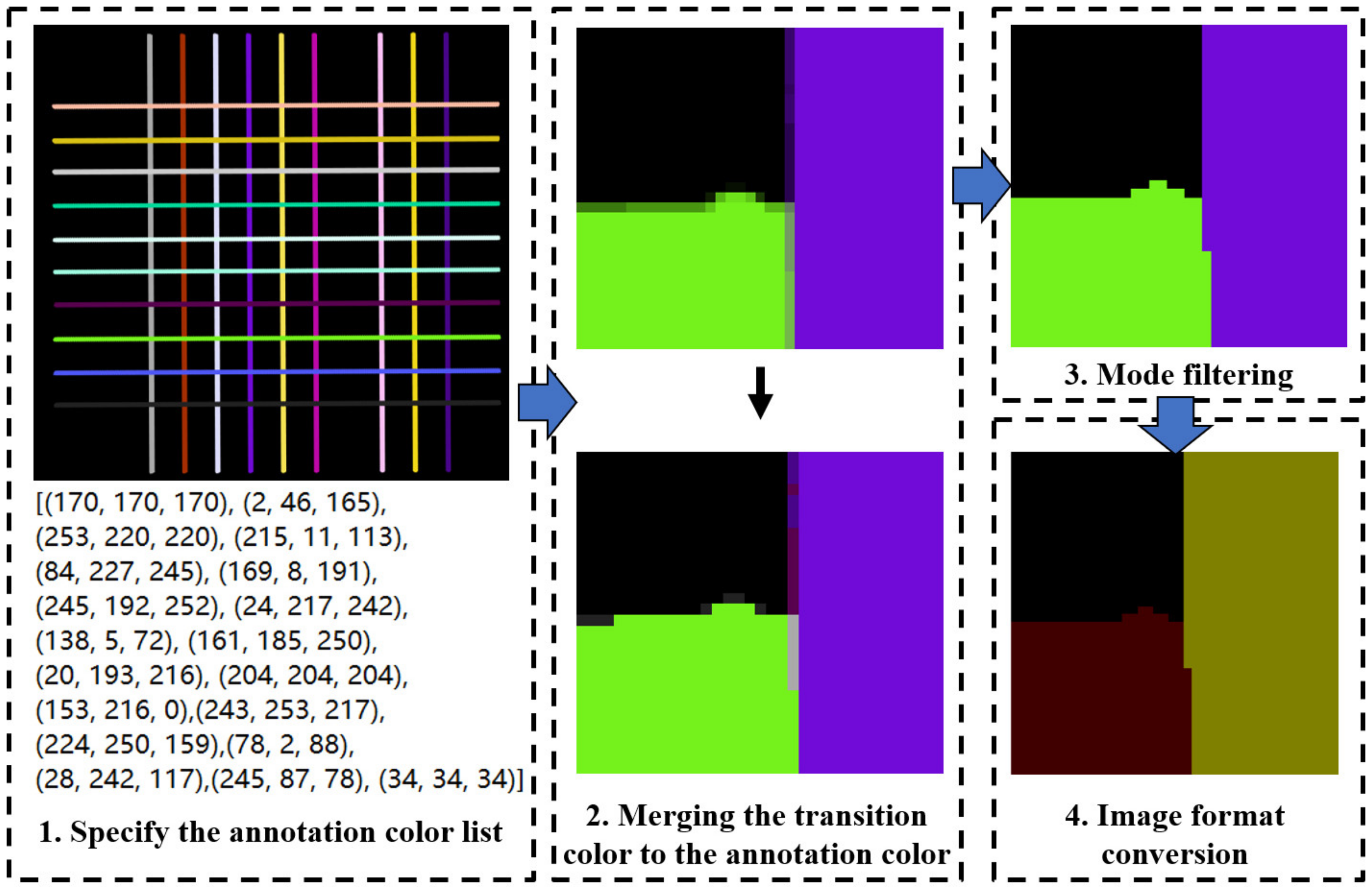
The transition color processing flow is shown in Figure 9 and includes four steps: specifying the annotation color list, merging the transition color to the annotation color, processing noise via mode filtering, and saving as a single-channel P-mode png format image.

Step 1: Specifying the annotation color list. This involves rendering the material ID map containing all target objects (rendering a picture containing all targets or rendering multiple pictures to cover all targets), using PS or a similar software tool to determine the RGB value of each annotation color, and entering them into the program.

Step 2: Merging the transition color with the annotation color. First, the pixel points whose values are neither the annotation color nor black are filtered; these are called transition color pixel points. Then, the “color distance” between the RGB color value of each transition color pixel point (the value range of each channel is 0–255) and the color value of each annotation color is calculated using formula (1), and the color value of the transition color pixel point is transformed into the annotation color with the smallest color distance.

$$D={\displaystyle \sum }_{i=R,G,B}^i{\left(T_i-L_i\right)}^2$$

(1)

In this formula, D refers to color distance, $T_i$ is the color value of channel i of the transition color pixel point, and $L_i$ is the color value of channel i of the annotation color.

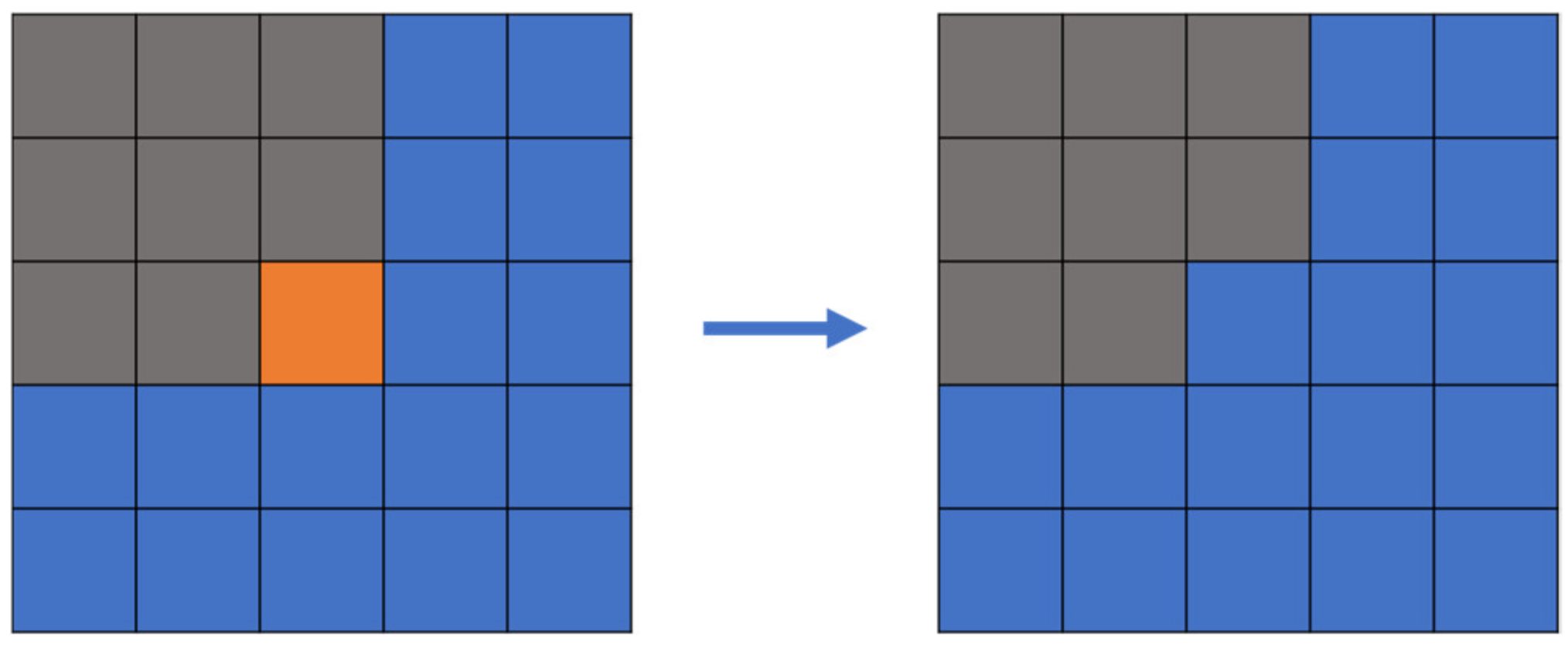
Step 3: Mode filtering. For a specified pixel point, its color value is defined as the color value that occurs most frequently in a square area within a given range, except black (as shown in Figure 10, which depicts mode filtering for the center pixel). After the color value merging in the previous step, some pixels are converted to the wrong annotation color, resulting in a small amount of dot-shaped or linear noise in the image, which must be eliminated using the mode filtering method. In this paper, 5 × 5 and a 3 × 3 sized mode filters were used in turn for all transition color pixels selected in the second step, to effectively eliminate noise, and the performance was good.

Step 4: Image format conversion. After completing the above three steps, the annotation image is still a three-channel color image and needs to be converted to a single-channel image, in order to meet the input requirements of the Mask R-CNN network. Additionally, the color value of the mask region of each instance in the image should be a continuous integer starting from 1, and the background color value should be 0. For the convenience of personnel inspection, the image is converted to a P-mode single-channel png image with a palette file, so that it can be presented in color. At this point, the annotation image processing is completed.

4. Synthetic Dataset Performance Comparison Experiment

In order to verify the performance of the synthetic dataset in the instance segmentation of rebar, this paper used different proportions of the real dataset and the synthetic dataset to form multiple mixed datasets, and used the same Mask R-CNN network with exactly the same training parameters to compare the datasets. The prediction performance was evaluated on the same test set, to check whether the synthetic dataset was equally effective compared to the real dataset.

4.1. Real Dataset Collection

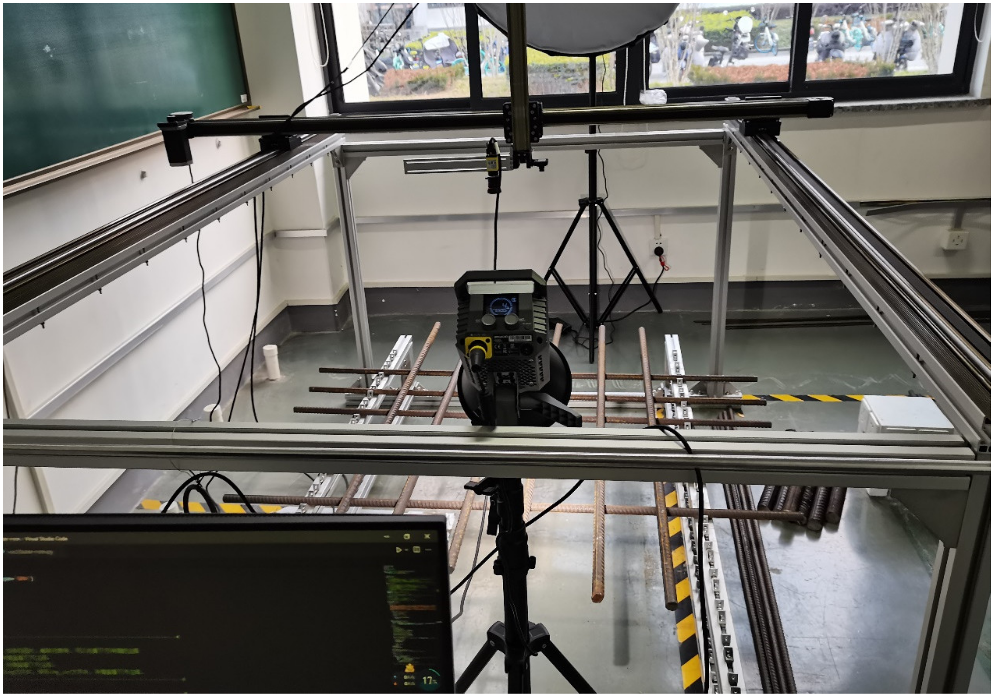
Real photographs of the rebar mesh were taken in an indoor laboratory environment using a Cognex CAM-CIC-12MR-8-GC industrial camera with an 8 mm-focal-length lens and a pixel resolution of 1006 × 759. Photographs were taken of rebar meshes consisting of 16 mm rebar with 20 mm rebar, and 20 mm rebar with 25 mm rebar, with a spacing of 150 mm to 200 mm. The rebar net was placed parallel to the ground on a rebar support frame, and the camera was installed on a motorized slider module on the rebar support frame with its axial direction perpendicular to the rebar net. The module moved the camera in three directions: front-to-back, left-to-right, and up-and-down. The shooting distance was 50 to 80 cm, with about 6 to 10 rebar pieces in the field of view. A total of 1500 shots were collected, of which 300 were taken with the light turned on. The location of the rebar was changed randomly or the rebar was rotated along the longitudinal axis, and the lighting conditions in the room were changed frequently by adjusting the blinds to enhance the diversity and generalization of the dataset during the shooting process. The image acquisition site is shown in Figure 11.

The object of the test set was a rebar mesh rebuilt with 16 mm, 20 mm, and 25 mm rebar pieces in the same environment. The photographs were taken using a mobile phone, with a resolution of 4608 × 3456, and the number of shots was 60. The axial direction of the rebar pieces in the photographs was parallel with or vertical to the edge of the picture, and the number of rebar pieces in each photograph was about 6 to 10.

4.2. Mask R-CNN Instance Segmentation Algorithm

The current deep learning algorithms for image segmentation can be divided into two categories: convolutional neural networks (CNNs) and transformers. In CNNs, the most commonly used networks include U-Net [14], SegNet [15], DeepLab V3+ [16], and Mask R-CNN [17]. Among them, Mask R-CNN is an instance segmentation network, and its applications in the civil engineering industry include rebar segmentation, road crack detection [18], and construction site safety management [19]. Its performance has been validated by many researchers. Therefore, Mask R-CNN was selected as the benchmark test network in this comparative experiment.

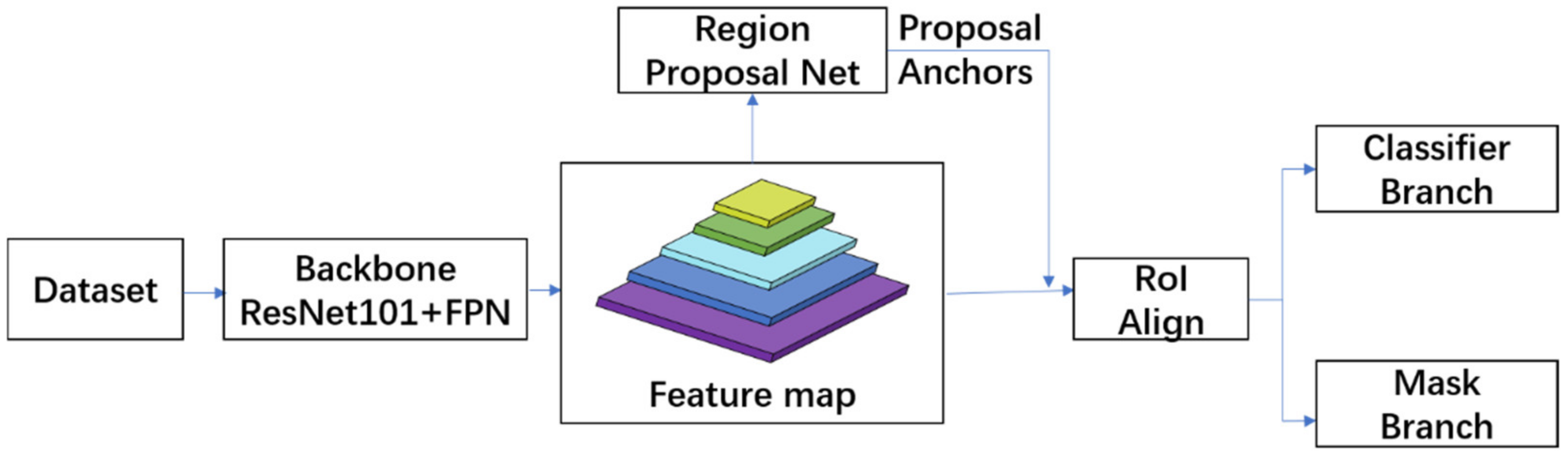
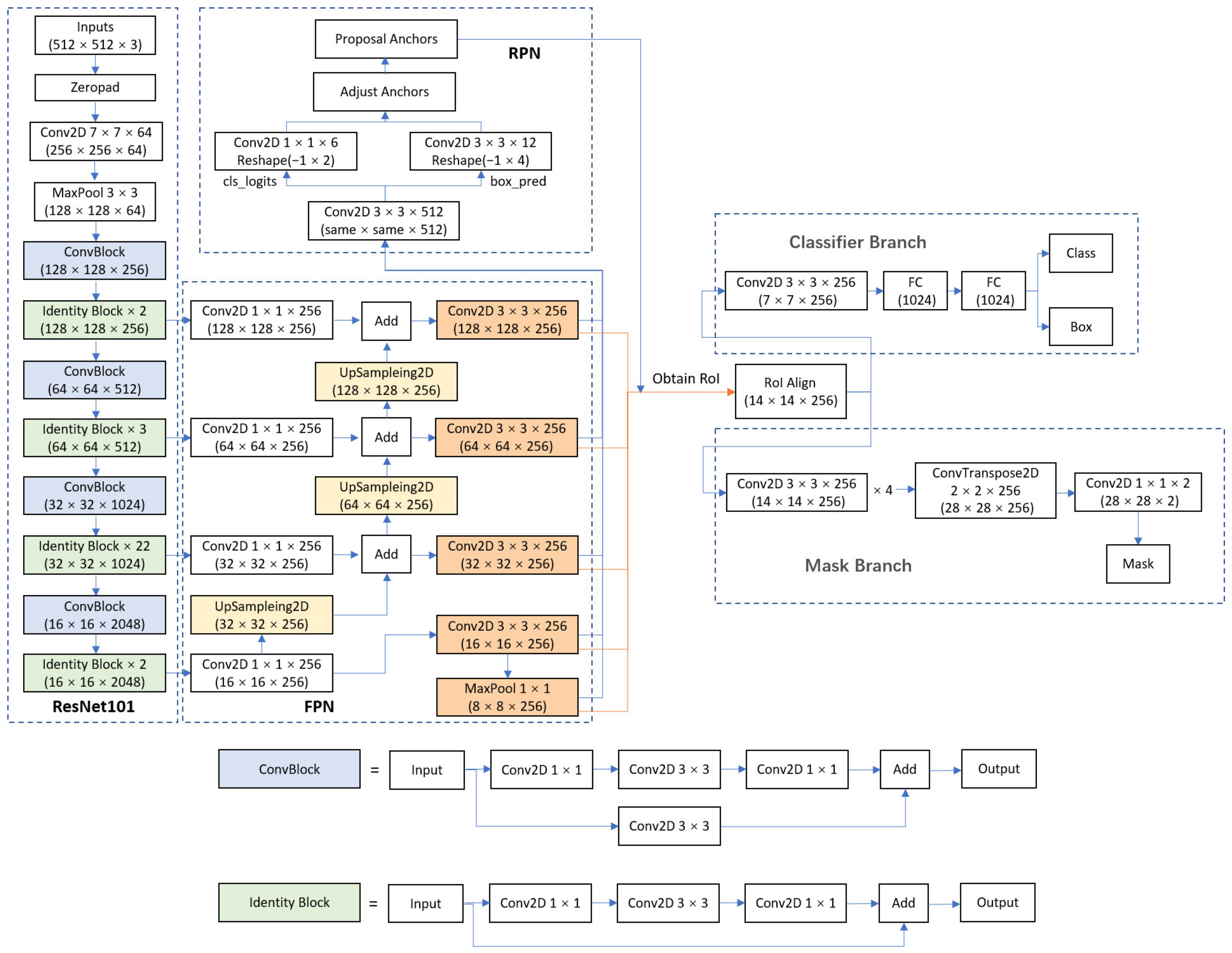
The sketch architecture of the Mask R-CNN network is shown in Figure 12. This network is based on Faster R-CNN [20] with a Mask prediction branch added, and the ROI Pooling layer of the original network was replaced with the ROI Align layer to achieve more accurate prediction. This algorithm has the functions of both object detection and instance segmentation. The detailed architecture of the Mask R-CNN network used in this paper is shown in Figure 13, for which we used ResNet-101-FPN as the backbone to execute the single classification instance segmentation task.

During training, the network first resizes the read-in images to 512 × 512 pixels and obtains feature maps at different scales through the backbone feature extraction network, to form a feature pyramid structure. Next, the region proposal net (RPN) generates proposal boxes at different scales based on the feature map and then uses these proposal boxes to intercept regions on the feature map at the corresponding scale. The intercepted regions are input into the RoI Align layer to be resized to a uniform size and then are input into the classification branch for classification, the box regression branch to predict the boxes, and the mask prediction branch for instance segmentation, respectively. Next, the losses are calculated and the training is completed via backpropagation. During prediction, the result is first output from the classifier branch and then input to the mask prediction branch for instance segmentation.

4.3. Training Environment and Training Parameters

The computer operating system used for training was Windows 10. The graphics cards used for training included Tesla V100, RTX 2080Ti, and GTX 1080Ti. The VRAM was 32 GB, 11 GB, and 11 GB, respectively. The software environment was set up as follows: TensorFlow-GPU1.13.2, Keras2.1.5, CUDA10.0, cuDNN7.4.1.5, and the programming language version was Python 3.6.

Each dataset was divided into a training dataset and a validation dataset, with proportions of 0.9 and 0.1, respectively; the test set comprised 60 real photographs captured using cell phones. Training was performed using a migration learning approach, by loading the COCO dataset pre-trained weights [21]. Models were trained with a learning rate of 0.0001, a batch size of 2, and a training epoch of 50 using an Adam optimizer, with a weight decay of 0.0001. Since rebar pieces are elongated objects, the anchor aspect ratio of RPN was set to 0.1, 5, and 10, and the sizes were set to 32, 64, 128, 256, and 512.

4.4. Model Evaluation Metrics

In order to evaluate the model and characterize the degree of matching between the prediction result and the real label, the accuracy, precision, recall, IoU, and F1 Score were used as the evaluation metrics. The calculation formula of each metric is as follows:

$$\mathrm{Accuracy}=\frac{\mathrm{TP}+\mathrm{TN}}{\mathrm{TP}+\mathrm{FP}+\mathrm{FN}+\mathrm{TN}}$$

(2)

$$\mathrm{Precision}=\frac{\mathrm{TP}}{\mathrm{TP}+\mathrm{FP}}$$

(3)

$$\mathrm{Recall}=\frac{\mathrm{TP}}{\mathrm{TP}+\mathrm{FN}}$$

(4)

$$\mathrm{IoU}=\frac{\mathrm{TP}}{\mathrm{TP}+\mathrm{FP}+\mathrm{FN}}$$

(5)

$$\mathrm{F}1\mathrm{Score}=\frac{2}{\frac{1}{\mathrm{Precision}}+\frac{1}{\mathrm{Recall}}}$$

(6)

In these formulas, TP (true positive) represents the number of pixels that are actually rebar and predicted to be rebar; TN (true negative) represents the number of pixels that are actually background and predicted to be background; FP (false positive) represents the number of pixels that are actually background and predicted to be rebar; and FN (false negative) represents the number of pixels that are actually rebar and predicted to be the background.

The values of the above five evaluation metrics range from 0 to 1, and the closer the value is to 1, the better the effect of the model.

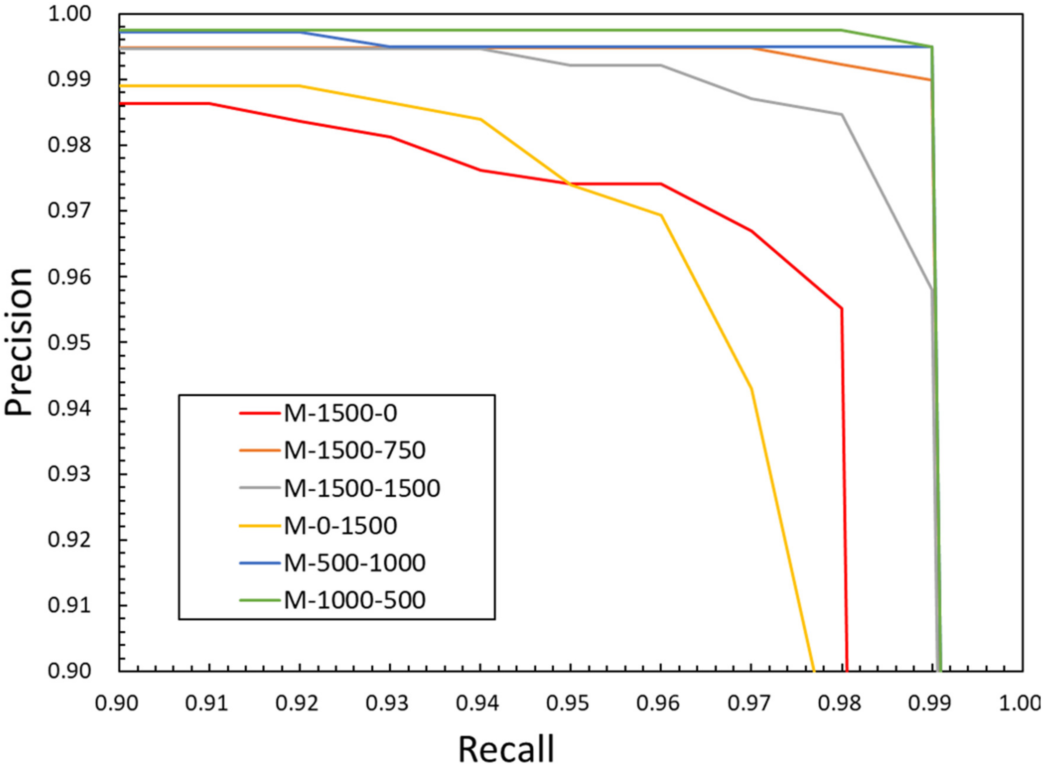
Precision–recall curves were used when the positive selection threshold was IoU = 0.5, to measure the performance of the models, which followed COCO dataset detection evaluation metrics [22]. Note that the definitions of precision and recall are different between Equations (3) and (4) and the precision–recall curves.

In addition, this study also used the rebar number recognition accuracy (Num_Accuracy) as an evaluation metric to compare and verify the evaluation results with the above five metrics, to improve the credibility of the test result evaluation. This was calculated as follows:

$$\mathrm{Num}\_\mathrm{Accuracy}=\frac{\mathrm{T}}{\mathrm{N}}$$

(7)

In the formula, N represents the total number of pictures in the test set, and T represents the number of pictures for which the number of rebar pieces is correctly predicted (that is, the number of rebar pieces predicted by the network is equal to the number of actual marked rebar pieces).

4.5. Training Dataset Configuration

A total of six training datasets were set up in this experiment, and six Mask R-CNN rebar instance segmentation models were trained using the same training parameters. The composition of each training set is shown in

Table 2. Training dataset configuration.

Model	Real Photograph Number	Synthetic Image Number
M-1500-0	1500	0
M-1500-750	1500	750
M-1500-1500	1500	1500
M-0-1500	0	1500
M-500-1000	500	1000
M-1000-500	1000	500

.

Among them, M-1500-0, M-1500-750, and M-1500-1500 were compared with each other to check the rationality of adding synthetic data to the real data and to show whether doing so improved the model’s prediction performance. M-1500-0, M-0-1500, M-500-1000, and M-1000-500 were compared with each other, to change the proportion of real data and synthetic data under the same dataset size and to study the rationality of using synthetic data to replace real data.

5. Experimental Results and Analysis

5.1. Data Processing of Evaluation Metrics

1. For the three metrics of accuracy, IoU, and F1_score, the prediction results of the Epoch50 weight file in the test set were used for model evaluation. Since the F1_score is the harmonic average of accuracy and recall, accuracy and recall are no longer involved in the calculation here, and are only used as reference metrics to more comprehensively show the model’s prediction performance.

2. We took the harmonic average of the three metrics obtained in the above steps to form a single index called the comprehensive metric, which is convenient for visual observation and comparative evaluation.

The calculation method of the harmonic average $H_n$ is as follows:

$$H_n=\frac{n}{{{\displaystyle \sum }}_{i=1}^n\frac{1}{x_i}}$$

(8)

In this formula, n represents the number of items involved in the calculation, and $x_i$ represents the value of the ith item involved in the calculation.

The purpose of the harmonic average here is to ensure that each sub-metric has the same contribution to the comprehensive metric and to avoid the comprehensive metric being controlled by a single metric.

5.2. Prediction Performance Comparison

Table 3. Prediction results of Epoch 50 weights.

Model	Accuracy	Precision	Recall	IoU	F1_Score
M-1500-0	0.935	0.922	0.809	0.756	0.860
M-1500-750	0.945	0.996	0.782	0.780	0.876
M-1500-1500	0.945	0.992	0.788	0.784	0.878
M-0-1500	0.933	0.990	0.742	0.736	0.848
M-500-1000	0.943	0.996	0.778	0.775	0.873
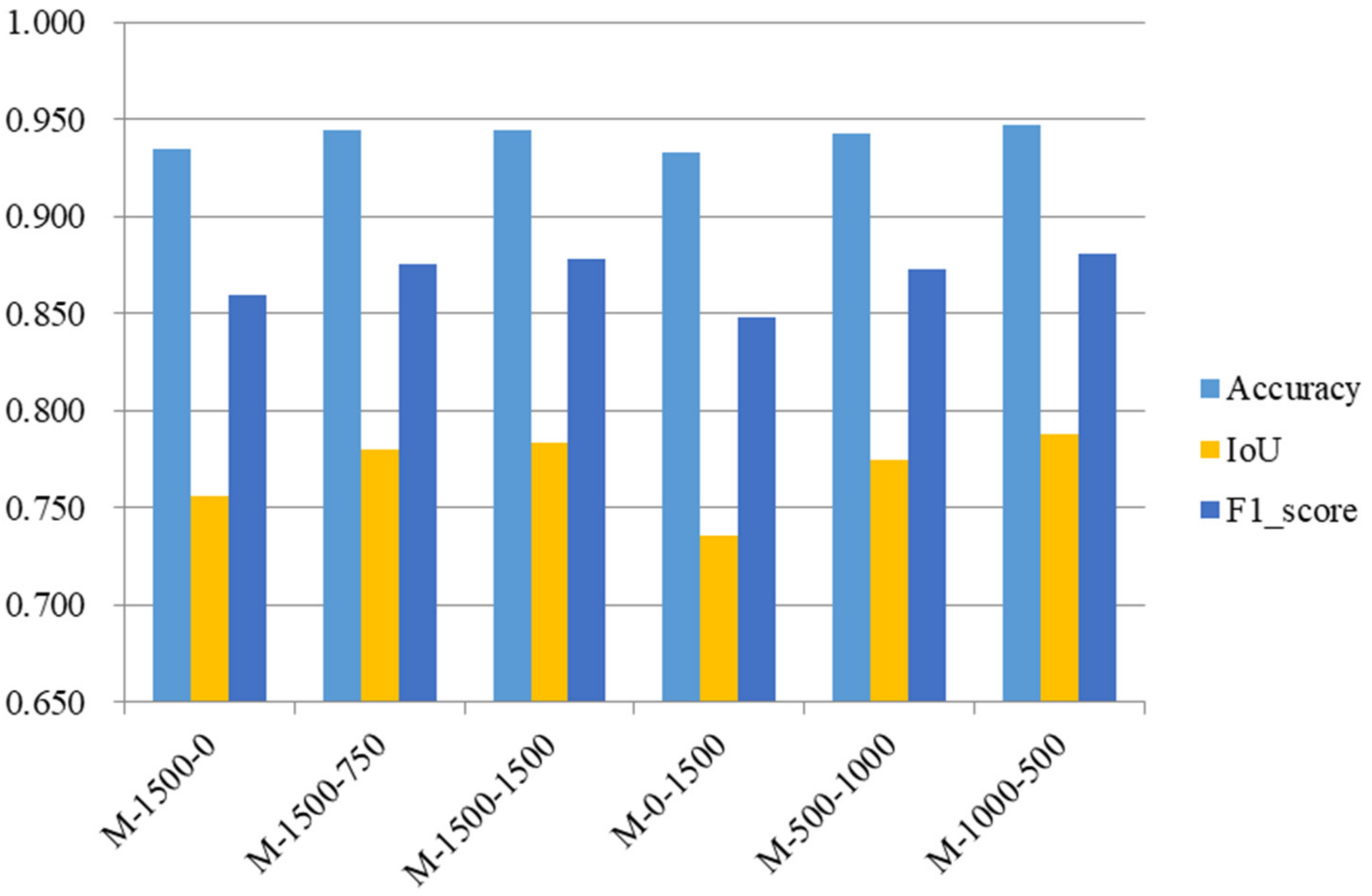
M-1000-500	0.947	0.993	0.792	0.788	0.881

shows the metrics of each model when the network prediction confidence was 0.7.

Figure 14 presents a bar chart that represents the data in Table 3, and shows the prediction performance of all six models trained on different training sets with the test set.

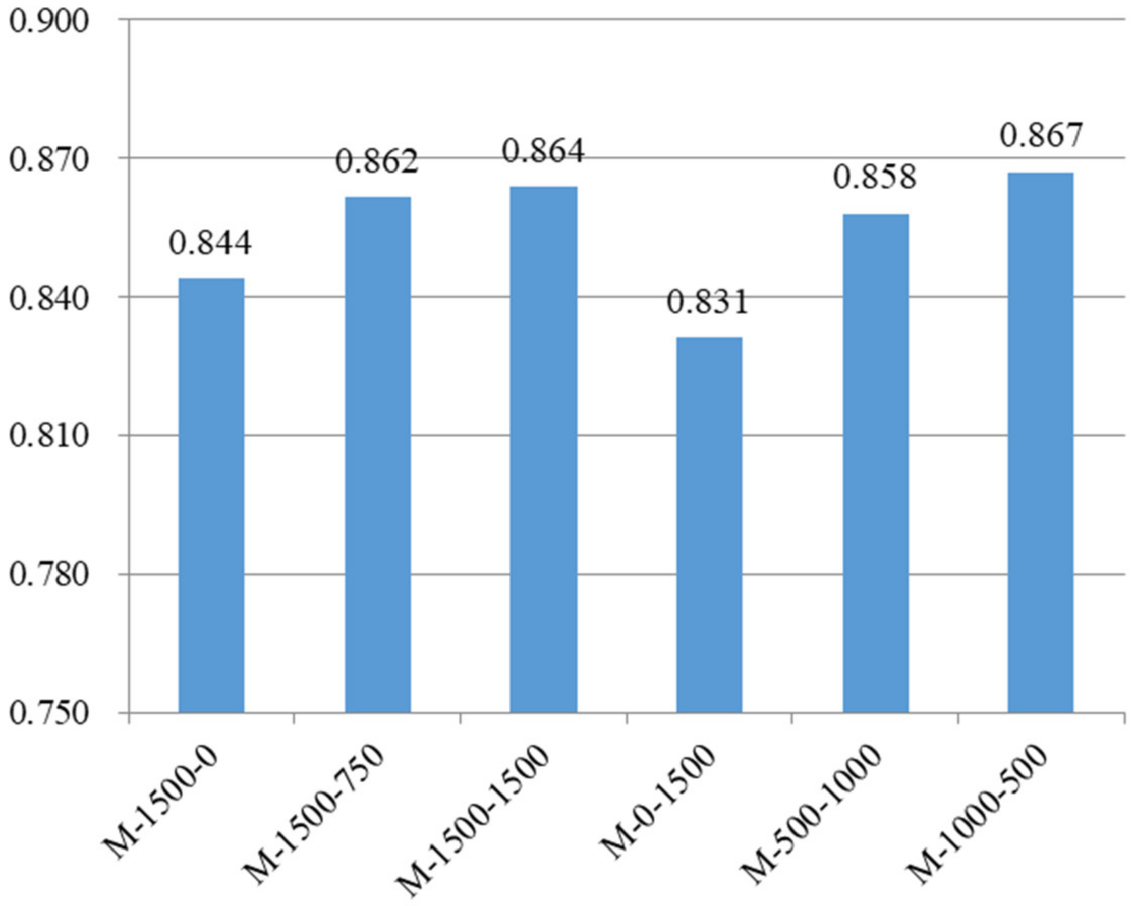
For the convenience of observation, we calculated the harmonic average of the accuracy, IoU, and F1_score in the above figure, and the comprehensive metric value was used to represent the prediction performance of each model, as shown in Figure 15. Additionally, the precision–recall curves of the six models are also shown in Figure 16.

The comparison of M-1500-0, M-1500-750, and M-1500-1500 shows that M-1500-750 and M-1500-1500 with synthetic images added to the training set had better prediction results with the test set than M-1500-0 with only real images, indicating that adding synthetic data to the real dataset improved the model’s prediction performance.

The comparison of M-1500-0, M-0-1500, M-500-1000, and M-1000-500 shows that with the same total number of 1500 images in the training set, M-500-1000 and M-1000-500, which contain both real and synthetic data in the training set, had better prediction results than M-1500-0, which contained only real images, and M-0-1500, which contained only synthetic images. This indicates that using synthetic images to replace some of the real images improved the model’s prediction performance. Additionally, M-0-1500 trained with synthetic images showed the lowest prediction performance with the test set but did not vary much from the other models, which proved the reasonableness and effectiveness of using synthetic images to train the model.

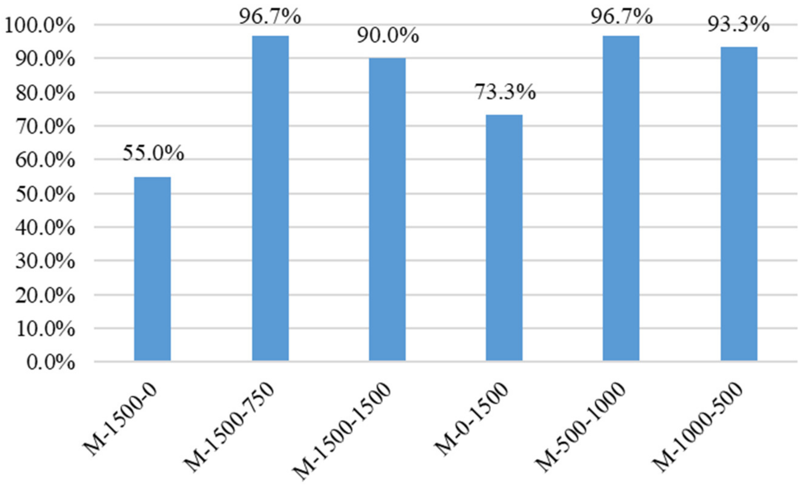
The rebar number recognition accuracy for each model in the test set is shown in Figure 17.

As can be seen in Figure 17, the recognition accuracy values of each model were compared with each other, and the trend was basically consistent with the previous evaluation metrics comparison (M-1500-750 and M-1500-1500 had better predictions results than M-1500-0, and M-500-1000 and M-1000-500 had better predictions results than M-1500-0 and M-0-1500), reflecting the reasonableness and effectiveness of using synthetic data to train the model.

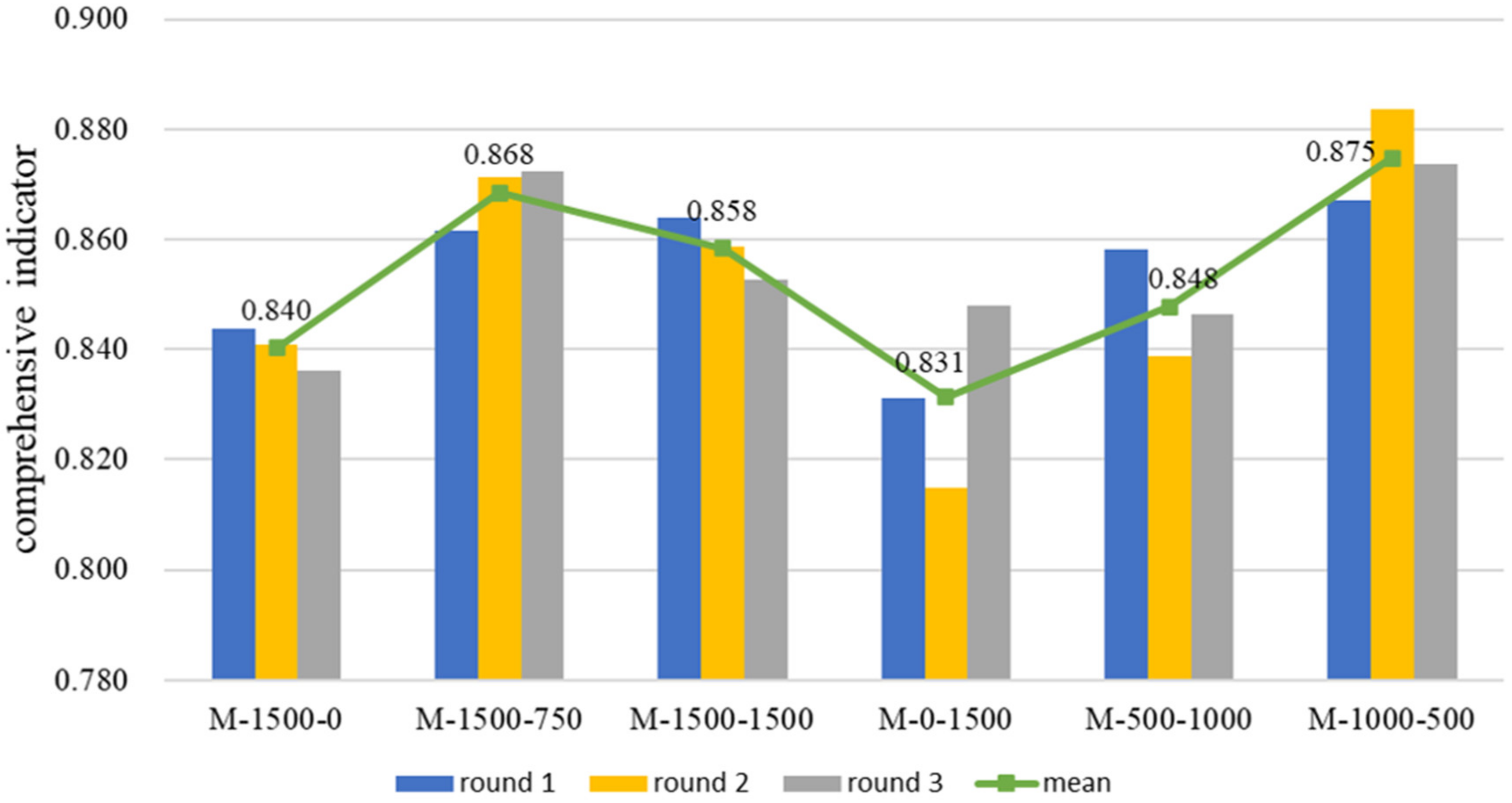
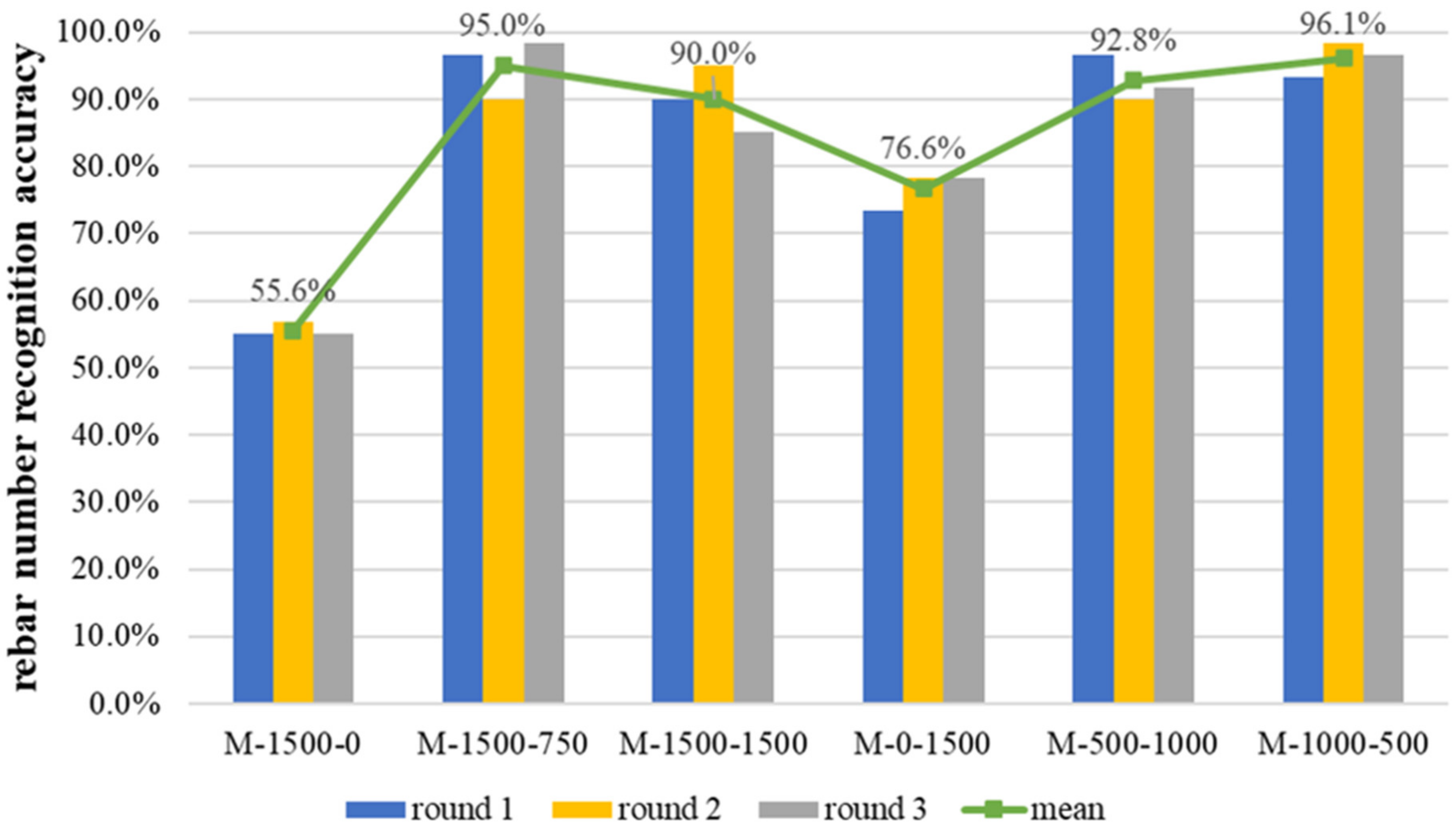
In order to verify the stability and credibility of the test results, the abovementioned test process was repeated twice, and the pictures in each training set were randomly selected each time. The model was trained with the same training parameters and tested using the same test set. The evaluation metrics of the three experiments are shown in Figure 18, and the comprehensive metric was used for evaluation. The rebar number recognition accuracy of the three trials is shown in Figure 19.

Figure 18 and Figure 19 show that the trends obtained from the three experiments were basically the same (M-1500-750 and M-1500-1500 had a better prediction accuracy than M-1500-0, and M-500-1000 and M-1000-500 had a better prediction accuracy than M-1500-0 and M-0-1500), reflecting the rationality and effectiveness of using synthetic data to train the model. This also proves the stability of the test results and strengthens their credibility. The reason for using the arithmetic mean of the results of the three repeated tests is that the mean value of the same metric was taken at this time. Moreover, there is no significant difference between the range of values of the same metric and the dispersion of the data in the same model in the repeated tests, and the difference between the harmonic mean and the arithmetic mean is small.

5.3. Analysis of Prediction Results

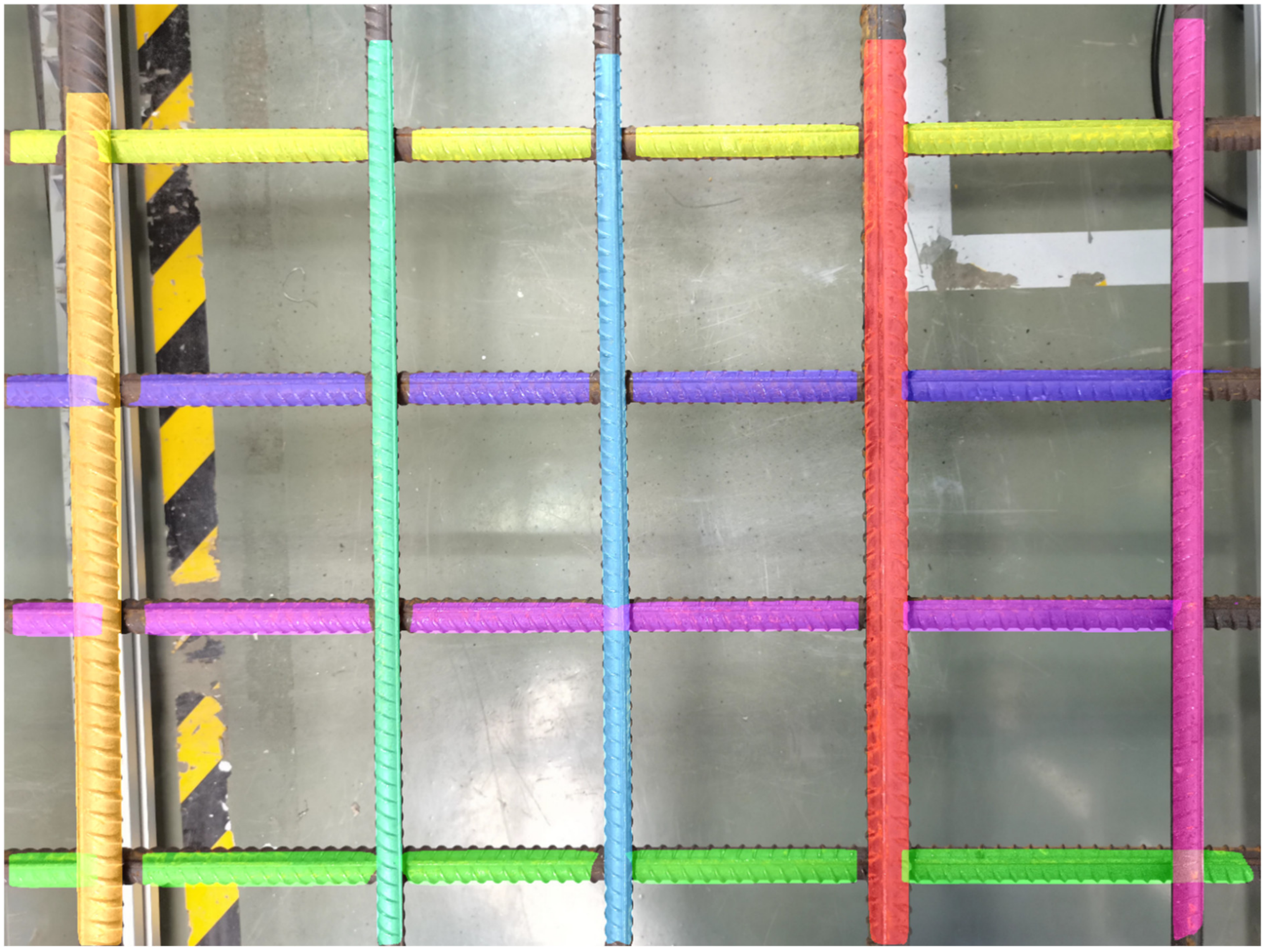
Taking M-1000-500 as an example, its prediction result with the test set is shown in Figure 20. In the figure, the part of the rebar covered by a colored mask is the rebar area identified by the Mask R-CNN network, and each rebar is marked with a different color.

It can be seen that the model had a good segmentation performance, the edge of the rebar is well-matched, and the intersection relationship of the rebar also has a certain recognition result. However, some rebar areas at the edge of the image and the intersections of the rebar were correctly segmented, which led to low IoU and recall values in the model evaluation metrics. However, the purpose of rebar segmentation is to identify the position and number of rebar pieces. Our results show that we could clearly distinguish their position and number, so the unrecognized image edges and rebar intersections had no effect on the identification results.

Therefore, from the perspective of recognition performance, the use of synthetic datasets is helpful for the accurate realization of rebar instance segmentation, and can replace or partially replace real datasets for the training of rebar instance segmentation models.

6. Discussion and Conclusions

1. This study proposes a rapid method of creating a synthetic rebar instance segmentation image dataset based on BIM and rendering software, which can not only quickly generate rebar images, but also automatically generate annotations, greatly reducing the workload and time costs of rebar dataset creation. The rendering and generation time of each image in the synthetic dataset is about 1 s, and the processing time of the annotation image is about 20 to 30 s, which is about three- to five-times faster than using manual annotation.

2. In this paper, six training datasets consisting of different numbers of real photographs and synthetic photographs were used, and six Mask R-CNN models were trained with the same training parameters, to compare the prediction performance for rebar instance segmentation. The prediction results of each model on the test set composed of real photographs illustrated that the synthetic dataset could effectively train the network model to identify the corresponding real target, which is reflected in the following: (1) adding synthetic data to the real dataset improved the model’s prediction performance; (2) the total number of datasets remained the same, and using synthetic data to replace part of the real data was better than using all-real or all-synthetic data. The reason for the improved performance of the network trained on the mixed dataset may be that the information in photographs in the dataset was richer and the trained network model was more generalizable.

3. This paper’s synthetic dataset creation method has a certain degree of versatility. It can be directly applied to the creation of datasets for any single-class instance segmentation task, by simply replacing the rebar model with a model of other objects, and can also be directly applied to synthetic dataset creation for multi-objective segmentation tasks.

4. In this study, two-dimensional segmentation of the rebar regions in photographs was achieved with the help of synthetic datasets. However, for automatic rebar tying and construction quality inspection in rebar projects, we need to identify actual 3D information such as the specific location, spacing, and diameter of the rebar. Further studies will be conducted in the future to address these shortcomings.