A Rapid Identification Technique of Moving Loads Based on MobileNetV2 and Transfer Learning

Abstract

Rapid and accurate identification of moving load is crucial for bridge operation management and early warning of overload events. However, it is hard to obtain them rapidly via traditional machine learning methods, due to their massive model parameters and complex network structure. To this end, this paper proposes a novel method to perform moving loads identification using MobileNetV2 and transfer learning. Specifically, the dynamic responses of a vehicle–bridge interaction system are firstly transformed into a two-dimensional time-frequency image by continuous wavelet transform to construct the database. Secondly, a pre-trained MobileNetV2 model based on ImageNet is transferred to the moving load identification task by transfer learning strategy for describing the mapping relationship between structural response and these specified moving loads. Then, load identification can be performed through inputting bridge responses into the established relationship. Finally, the effectiveness of the method is verified by numerical simulation. The results show that it can accurately identify the vehicle weight, vehicle speed information, and presents excellent strong robustness. In addition, MobileNetV2 has faster identification speed and requires less computational resources than several traditional deep convolutional neural network models in moving load identification, which can provide a novel idea for the rapid identification of moving loads.

1. Introduction

Moving load is the main external load acting on the bridge [1,2]. Due to the inefficient supervision of overweight vehicles, bridge collapse accidents caused by overweight vehicles have occurred occasionally in recent years [3,4,5]. Therefore, the accurate and rapid recognition of moving loads is beneficial to the early warning and control of the overweight vehicle, thereby ensuring the safe operation of the bridge [6,7]. Traditional moving loads identification method primarily rely on a bridge weigh-in-motion (WIM) system. However, WIM may harm the road surface, and the sensor is prone to be damaged under long-term moving load, which increases the operation and maintenance costs [8]. Therefore, it is urgent to indirectly identify the moving load using the dynamic response by a more efficient and economic method, i.e., moving load identification (MLI) methods.

MLI methods can roughly be classified into two categories, i.e., intelligent optimization methods and machine learning methods. Among them, intelligent optimization methods compute the optimal solution of the loss function to obtain the load parameters with the smallest loss function [9]. For example, Wang et al. [10] applied simulated annealing algorithm to identify multi-axis moving train loads, and the experimental results demonstrated that the proposed method exhibits excellent robustness and accuracy. Pan et al. [11] proposed a moving loads identification method based on the firefly algorithm, in which, vehicle load information can be accurately identified with only a small number of sensors. Liu et al. [12] recognized the constant component of the moving load with the help of particle swarm algorithm and used the hybrid measurement response to further improve the identification accuracy. Ali R. Vosoughi et al. [13] applied a genetic algorithm for moving load identification by defining a root mean square error function between the measured and calculated responses, and the results showed that the accuracy and efficiency of this method higher than the Newmark’s method. Although the intelligent optimization methods can effectively obtain the moving load information from the bridge response, the optimization process often requires searching a huge solution space, which leads to computational inefficiency and is not conducive to the rapid identification of moving loads [14].

With the rapid development of artificial intelligence, machine learning (especially deep learning) has shown great advantages in feature extraction, target detection, and recognition [15], etc., and is also widely applied in moving load identification. For instance, Yang et al. [16] applied a neural network to acquire the information of moving load through structural dynamic strain and discussed the influence of activation function on identification accuracy. Zhou et al. [17] developed a moving load identification algorithm, which converted the bridge acceleration response into a two-dimensional map as the network input. Chen et al. [18] reconstructed and located impact load based on deep convolution recurrent neural network and feature learning, which avoided the infeasibility and ill-posedness of nonlinear structure when identifying random impact loads. Zhang [19] applied a long short-term memory neural network to obtain the information of moving loads through the dynamic responses of the bridge, and the results revealed that the information of the moving load can be recognized synchronously with great accuracy. The above literature confirms the great potential of machine learning methods in the accurate and efficient identification of moving loads. However, these machine learning methods often encounter a heavy computational burden, due to the large model parameters and complex network structure, which leads to an inefficient identification process.

Fortunately, lightweight convolutional neural network has a faster identification speed. Compared with traditional deep convolutional neural network models, separable convolution is used in lightweight convolutional neural network model, which greatly reduces the model parameters without sacrificing the accuracy of the model. As a lightweight convolutional neural network model with superior performance [20], the MobileNetV2 model has not yet been used in moving load identification. Therefore, this paper proposes a moving load identification method based on MobileNetV2 and transfer learning, which has faster identification speed and requires less computing resource. Concretely, the continuous wavelet transform (CWT) is first applied to convert the dynamic responses of vehicle-bridge interaction (VBI) system into images to construct the data set for the moving load identification task. Secondly, a pre-trained MobileNetV2 model is applied to the load identification task through transfer learning strategy to enhance the efficiency of the model. Then, the information of moving loads can be acquired through inputting responses of bridge into the completely trained model. Finally, the feasibility of the method is demonstrated in the numerical modeling case.

The major contributions of this paper in comparison with the published literature are summarized in the following.

(1)

MobileNetV2 has been introduced into moving load identification to improve the identification efficiency. Case study shows that the MobileNetV2 has faster identification speed and requires less computational resources than traditional deep convolutional neural network models in moving load identification.

(2)

The influence of several types of dynamic response on moving loads identification is discussed. The results demonstrate that the displacement response may be the most suitable input for vehicle load identification, while acceleration response may be more suitable for vehicle speed identification, which provides a guideline for the accurate identification of moving loads.

This paper is organized as follows. In Section 2, the theoretical background involved in this paper is introduced. In Section 3, the process of this method is described. The case study of identification task is conducted in Section 4. In Section 5, the performance of this method is discussed and analyzed. In Section 6, several conclusions are described.

2. Theoretical Background

In this section, firstly, the VBI dynamic model is described. Then, the popular deep convolutional neural network (DCNN) models and lightweight convolutional neural network models are introduced. Finally, the basic concept of transfer learning is introduced.

2.1. The VBI Dynamic Model

The VBI dynamic model is a complex dynamic system, composed of moving vehicles and bridges. In this subsection, the Newmark-β method is used to solve the dynamic equation of the VBI model, thereby obtaining the dynamic response of the model.

2.1.1. Road Surface Roughness

PSD function is used to transformed road surface roughness from spatial frequency domain to the circular frequency domain [21], as follows:

$$\left\{\begin{array}{l}{S}_{rr}\left(\mathrm{\Omega }\right)=S_{rr}\left({\mathrm{\Omega }}_0\right){\left(\mathrm{\Omega }/{\mathrm{\Omega }}_0\right)}^{-2}\hspace{1em}\left(\mathrm{\Omega }\le {\mathrm{\Omega }}_0\right)\\ S_{rr}\left(\mathrm{\Omega }\right)=S_{rr}\left({\mathrm{\Omega }}_0\right){\left(\mathrm{\Omega }/{\mathrm{\Omega }}_0\right)}^{-1.5}\hspace{1em}\left(\mathrm{\Omega }>{\mathrm{\Omega }}_0\right)\end{array}\right.$$

(1)

Road surface roughness can be calculated by the inverse Fourier transform of the road surface roughness spectrum, as follows [22]:

$$r\left(x\right)={\displaystyle \sum _{i=1}^N\sqrt{\Delta n}·2^k·{10}^{-3}·\left(\frac{n_0}{i·\Delta n}\right)}\cos \left(2\pi i·\Delta nx+{\varphi }_i\right)$$

(2)

where r(x) is a variable about bridge length L, $\Delta n=1/L$; N is the number of data points, and k is a constant integer increasing from 3 to 9. ${\varphi }_i$ is the random phase angle distributed uniformly between 0 and 2π.

2.1.2. The Vehicle Model

In this section, a vehicle model is established, which involves mass, spring, and damper [23]. The influence of road roughness on vehicle-bridge interaction vibration are considered, as shown in Figure 1. These assumptions are used in the VBI dynamic model: (i) the vehicle is traveling on the bridge with a constant speed v; (ii) the wheel is always in contact with the beam by point contact; (iii) the displacement of the wheel and the beam at the contact point is consistent.

According to the Newton’s second law, the vibration equation of the vehicle can be written as:

$$m_v{\ddot{y}}_v=F_{vb}-F_G$$

(3)

where $m_v$ and $y_v$ are the vehicle weight and vehicle displacement, respectively; $F_G$ and $F_{vb}$ are the vehicle gravity and the interaction force, respectively. $F_{vb}$ can be calculated by:

$$F_{vb}=-k_v(y_v-y_{bc}-r)-c_v({\dot{y}}_v-{\dot{y}}_{bc}-\dot{r})$$

(4)

where $k_v$, $c_v$ and $y_{bc}$ are spring stiffness, the damping, the bridge deflection, respectively. $y_{bc}$ can be calculated by:

$$y_{bc}={\mathit{N}}_b·{\mathit{y}}_b$$

(5)

where ${\mathit{y}}_b$ denotes the global displacement vector of the bridge, ${\mathit{N}}_b$ denotes the bridge shape function.

Combining the Equations (3)–(5), we can obtain:

$$m_v{\ddot{y}}_v-{\mathit{C}}_{vb}·{\dot{\mathit{y}}}_b+c_v{\dot{y}}_v-{\mathit{K}}_{vb}·{\mathit{y}}_b+k_v{y}_v=F_{vr}-F_G$$

(6)

where ${\mathit{C}}_{vb}=c_v·{\mathit{N}}_b$, ${\mathit{K}}_{vb}=c_v·{\dot{\mathit{N}}}_b+k_v·{\mathit{N}}_b$, $F_{vr}=c_v\dot{r}+k_{v}r$ are the vehicle additional damping, stiffness, and load terms, respectively.

2.1.3. The Bridge Model

Under vehicle load, bridge dynamic equation can be expressed as:

$${\mathit{M}}_b{\ddot{\mathit{y}}}_b+{\mathit{C}}_b{\dot{\mathit{y}}}_b+{\mathit{K}}_b{\mathit{y}}_b=-{\mathit{F}}_{bv}$$

(7)

where ${\mathit{M}}_b$ is bridge mass matrices, ${\mathit{C}}_b$ is bridge damping matrices, and ${\mathit{K}}_b$ is bridge stiffness matrices; ${\mathit{F}}_{bv}$ is the equivalent nodal force of ${\mathit{F}}_{bv}$. It has the following relationship:

$${\mathit{F}}_{bv}={\mathit{N}}_b^T·{\mathit{F}}_{bv}={\mathit{N}}_b^T·F_{vb}$$

(8)

Substituting Equations (8) and (4) into Equation (7), we can obtain:

$${\mathit{M}}_b{\ddot{\mathit{y}}}_b+\left({\mathit{C}}_b+{\mathit{C}}_{bb}\right){\dot{\mathit{y}}}_b-{\mathit{C}}_{bv}·{\dot{\mathit{y}}}_v+\left({\mathit{K}}_b+{\mathit{K}}_{bb}+{\mathit{K}}_{bc}\right){\mathit{y}}_b-{\mathit{K}}_{bv}·y_v=-{\mathit{K}}_b^T·F_{vr}$$

(9)

where ${\mathit{C}}_{bb}={\mathit{N}}_b^T·c_v·{\mathit{N}}_b$, ${\mathit{C}}_{bv}={\mathit{N}}_b^T·c_v$, ${\mathit{K}}_{bb}={\mathit{N}}_b^T·k_v·{\mathit{N}}_b$, ${\mathit{K}}_{bc}={\mathit{N}}_b^T·c_v·{\dot{\mathit{N}}}_b$ and ${\mathit{K}}_{bv}={\mathit{N}}_b^T·k_v$ are the bridge additional damping and stiffness, respectively.

2.1.4. The VBI Dynamic Model

The VBI dynamic equation can be obtained by combining Equations (6) and (9) in the matrix form:

$$\left[\begin{array}{cc}{\mathit{M}}_b& 0\\ 0& m_v\end{array}\right]\left[\begin{array}{c}{\ddot{\mathit{y}}}_b\\ {\ddot{y}}_v\end{array}\right]+\left[\begin{array}{cc}{\mathit{C}}_b+{\mathit{C}}_{bb}& -{\mathit{C}}_{bv}\\ -{\mathit{C}}_{vb}& c_v\end{array}\right]\left[\begin{array}{c}{\dot{\mathit{y}}}_b\\ {\dot{y}}_v\end{array}\right]+\left[\begin{array}{cc}{\mathit{K}}_b+{\mathit{K}}_{bb}+{\mathit{K}}_{bc}& -{\mathit{K}}_{bv}\\ -{\mathit{K}}_{vb}& k_v\end{array}\right]\left[\begin{array}{c}{\mathit{y}}_b\\ y_v\end{array}\right]=\left[\begin{array}{c}-{\mathit{N}}_b^T·F_{vr}\\ F_{vr}-F_G\end{array}\right]$$

(10)

To improve the computational efficiency, the model synthesis method is used to reduce the computational degrees of freedom of the bridge, and the vibration equations of the VBI dynamic model are rewritten as follows:

$$\left[\begin{array}{cc}\mathit{I}& \mathrm{𝟎}\\ \mathrm{𝟎}& m_v\end{array}\right]\left[\begin{array}{c}{\ddot{q}}_b\\ {\ddot{y}}_v\end{array}\right]+\left[\begin{array}{cc}{\overline{\mathit{C}}}_b+{\mathbf{\Phi }}_b^T{\mathit{C}}_{bb}{\mathrm{\Phi }}_b& -{\mathbf{\Phi }}_b^T{\mathit{C}}_{bv}\\ -{\mathit{C}}_{vb}{\mathbf{\Phi }}_b& c_v\end{array}\right]\left[\begin{array}{c}{\dot{q}}_b\\ {\dot{y}}_v\end{array}\right]+\left[\begin{array}{cc}{\overline{\mathit{K}}}_b+{\mathbf{\Phi }}_b^T\left({\mathit{K}}_{bb}+{\mathit{K}}_{bc}\right){\mathbf{\Phi }}_b& -{\mathbf{\Phi }}_b^T{\mathit{K}}_{bv}\\ -{\mathit{K}}_{vb}{\mathbf{\Phi }}_b& k_v\end{array}\right]\left[\begin{array}{c}{q}_b\\ y_v\end{array}\right]={\mathit{F}}_R+{\mathit{F}}_G$$

(11)

where Φ_b is the modal shape matrix of the bridge.

$${\mathit{F}}_R=\left[\begin{array}{c}-{\mathbf{\Phi }}_b^T{\mathit{N}}_b^T·F_{vr}\\ F_{vr}\end{array}\right], {\mathit{F}}_G=\left[\begin{array}{c}\mathrm{𝟎}\\ F_G\end{array}\right]$$

Let $\mathit{M}=\left[\begin{array}{cc}{\mathit{M}}_b& \mathrm{𝟎}\\ \mathrm{𝟎}& m_v\end{array}\right]$, $\mathit{C}=\left[\begin{array}{cc}{\mathit{C}}_b+{\mathit{C}}_{bb}& -{\mathit{C}}_{bv}\\ -{\mathit{C}}_{vb}& {\mathit{C}}_v\end{array}\right]$, $\mathit{K}=\left[\begin{array}{cc}{\mathit{K}}_b+{\mathit{K}}_{bb}+{\mathit{K}}_{bv}& -{\mathit{K}}_{bv}\\ -{\mathit{K}}_{vb}& k_v\end{array}\right]$, ${\mathit{F}}_{eq}={\mathit{F}}_G+{\mathit{F}}_R$.

According to the Newmark-β method, one can obtain:

$${\mathit{K}}_{eq}{y}_i={\mathit{F}}_{eq}$$

(12)

where

$$\begin{array}{c}{\mathit{F}}_{eq}=\mathit{F}+\mathit{M}[\frac{1}{\beta \Delta t^2}{y}_i+\frac{1}{\beta \Delta t}{\dot{y}}_i+(\frac{1}{2\beta }-1){\ddot{y}}_i]+\mathit{C}[\frac{\gamma }{\beta \Delta t}{y}_i+\frac{\gamma }{\beta }-1){\dot{y}}_i+(\frac{\gamma }{\beta }-2){\ddot{y}}_i]\\ {\mathit{K}}_{eq}=\mathit{K}+\frac{1}{\beta \Delta t^2}\mathit{M}+\frac{\gamma }{\beta \Delta t}\mathit{C}\end{array}$$

According to the Newmark-β method, when the initial displacement, velocity, and acceleration at the initial time are given, the response of the system at any time can be determined based on Equation (12), and the complete time series data for dynamic response can be obtained.

2.2. Deep Convolutional Neural Network

2.2.1. Popular Models of DCNN

In 1998, Lecun et al. [24] constructed the first convolutional neural network model (LeNet-5), which has excellent identification performance in handwritten font identification tasks. In 2012, Krizhevsky and Hinton [25] proposed AlexNet, which won first place in that year’s ImageNet Visual Recognition Challenge. Since then, various artificial intelligence applications based on DCNN have been merged, and DCNN has developed rapidly. Some new models have been proposed, which can be divided into the branchless model, such as VGG, and modular stacked models, such as GoogleNet, ResNet, and DenseNet.

VGGNet [26] constructs a deeper network structure based on AlexNet network to improve the learning ability of image features. Meanwhile, VGGNet stacks smaller convolution kernels to reduce network parameters and iterations. VGGNets are still widely used in image feature extraction due to their excellent performance. In the same year, Google launched GoogleNet [27], which used far less network parameters than VGGNet. Therefore, it takes up less memory and computing resources in computing. It also used a modular network structure containing convolution kernel parallel merging. After years of optimization and improvement, several versions have been derived.

ResNet [28] adopts the same modular stack structure as VGGNet and introduces a novel residual structure to greatly improve the fitting ability and overcome the degradation problem of deep neural network. Subsequently, DenseNet [29] introduces a dense block structure to reuse the features of each layer of feature map, thereby improving the transmission of features in the network, improving the identification efficiency of the network, and reducing the number of network parameters.

Although the deep convolutional network model has excellent performance, its computational efficiency is low, due to the complex network structure, which makes DCNNs difficult to widely applied in practical engineering.

2.2.2. Lightweight Convolutional Neural Networks

Lightweight convolutional neural networks aim to reduce computational storage and increase recognition speed. Lightweight convolutional neural networks mainly include ShuffleNet series and MobileNet series. Howard et al. [30] proposed MobileNetV1, which uses a straight network structure and replace the deep separable convolution instead of traditional convolutional layers. By this improvement, the model parameters can be greatly reduced while ensuring the computational accuracy of the network. Then, Sandler et al. proposed MobileNetV2, which adopts the deep separable convolution instead of the traditional standard convolution and adds the inverted residuals block and linear bottlenecks structure. Therefore, MobileNetV2 reduces the number of model parameters while ensuring accuracy. The convolution process of MobileNetV2 is shown in Figure 2. Due to the excellent performance and lightweight size, MobileNet series models are often used in various recognition fields [31,32,33,34]. Because the moving load identification needs to respond rapidly to the vehicle information in driving, this paper introduces MobileNetv2 into the moving load identification.

2.3. Transfer Learning

The main concept of transfer learning is to utilize data from similar fields to solve the problem of data shortage in target fields. Its goal is to utilize the knowledge learned from an original environment to help learn tasks in a new environment. Depending on the requirements for transfer into the target domain, it can be classified as the following forms [35]: (1) instance transfer; (2) feature representation transfer; (3) parameter transfer; (4) relational knowledge transfer.

The strong transferability of neural network model greatly improves the applicability of transfer learning in the field of deep learning. Compared with the general transfer learning method, the transfer learning strategy in DCNNs transfers the shallow feature extraction ability (i.e., texture, edge feature, etc.) in the source domain to the target domain. Therefore, fine-tuning is commonly used in DCNNs for transfer learning. Specifically, it is to freeze the front several layers network of the pre-trained model, retrain the remaining layers, and replace the task classifier to match the new learning task when the new dataset has a small amount of data, and it is significantly different from the training dataset used by the pre-trained model. An example of transfer learning is shown in Figure 3.

3. The Proposed Method

This paper proposes a moving load identification method based on MobileNetV2 and transfer learning, which identify the moving load information from responses of bridge, respectively. The training of DCNNs needs to optimize a large number of parameters and construct sufficient samples, and it will take a lot of time to train the model from scratch. Therefore, this paper adopts transfer learning strategy. The implementation process of this method is shown in Figure 4, including the following steps:

(1)

Responses acquisition and pre-processing. By solving the VBI dynamic equation, the responses of bridge corresponding to different vehicle parameters are obtained. In order to meet the input requirements of DCNN, the CWT is applied to transform the response into a time-frequency map. The formula of CWT is as follows:

$$WT\left(a,b\right)=\frac{1}{\sqrt{a}}{\displaystyle {\int }_{-\infty }^{\infty }x\left(t\right)·\psi \left(\frac{t-b}{a}\right)}dt$$

(13)

where $a$ is the scaling factor which can control the expansion of wavelet, $b$ denotes the shifting factor that identifies its location, and $\psi$ denotes the mother wavelet. In this paper, Complex Morlet wavelet is used as the mother wavelet $\psi$ because it has good resolution in both time and frequency domains [36]. Both the scaling factor $a$ and the shifting factor $b$ are set to 3.

(2)

Dataset construction. The size of normalized image samples is adjusted to the input size of the MobileNetV2 model. On this basis, all image samples are labelled with the corresponding VBI system parameters, thus forming the sample library of displacement, velocity, and acceleration responses for the moving load identification task. Then, the samples are divided into the training set, validation set and test set with the ratio as 8:1:1. The network is trained by the training set, the network is verified by the validation set, and the performance of the network is evaluated by the test set.

(3)

Model training. A pre-trained MobileNetV2 model is used to moving load identification tasks. On this basis, the hyperparameters (batch size, learning rate, epoch, etc.) of model is adjusted to optimize the network performance. Meanwhile, the bottlenecks of the MobileNetV2 model are retrained, and the original 1000-class target classifiers are replaced with the 5-class target classifiers required for moving load identification in this task.

(4)

Moving load identification. Test set samples are input to the trained MobileNetV2 model to obtained information of moving loads and to evaluate the identification performance of the network.

4. Case Study

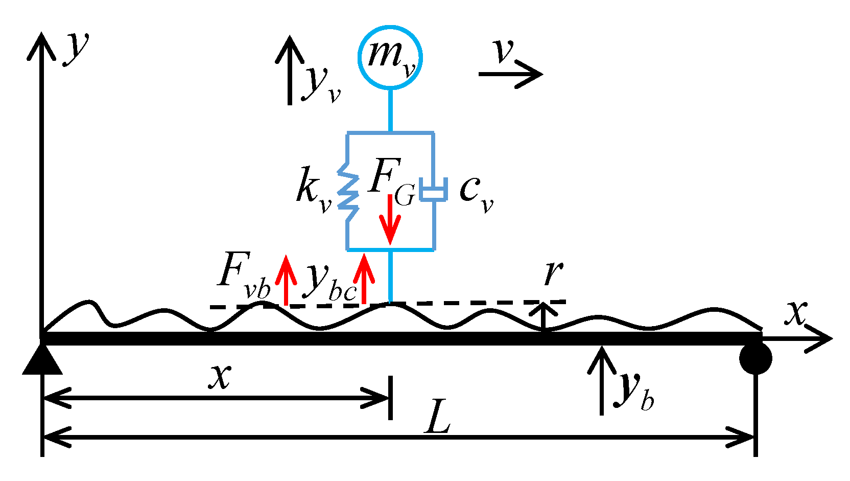
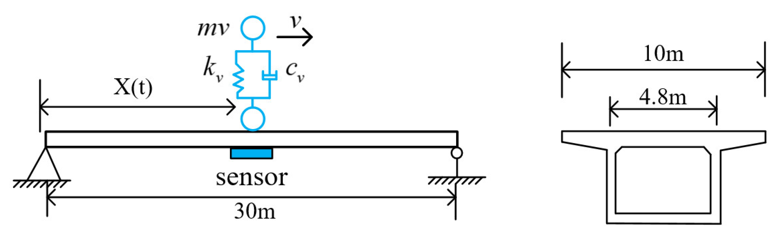
In order to verify the feasibility of the proposed method, the VBI system with single degree of freedom is taken as the object in this paper. According to the VBI dynamic equation, a sufficient sample database is constructed to perform moving load identification tasks.

4.1. The Numerical Model

In this paper, a 30 m concrete simply supported, single-span bridge is established to verify the method, as shown in Figure 5. The main beam is simulated by beam188 element [37,38,39] with concrete specification of C50. The elastic modulus is 3.40 × 10⁴ MPa, and Poisson ratio is 0.2, mass density is 2600 kg/m³. The single-wheeled vehicle model is simulated by spring element. The spring stiffness of vehicle is set to $k_v=190 \mathrm{kN}/\mathrm{m}$ and the damping of the vehicle is $c_v=5 \mathrm{kN}·\mathrm{m}/\mathrm{s}$. The information for the vehicle is designed according to the required load conditions.

4.2. Vehicle Weight Identification

Acquisition of vehicle weight information is critical to the safe operation of bridges. In this section, vehicle weight is classified into 5 categories from light to heavy (i.e., A, B, C, D, E), and the vehicle weight classification table is shown in

Table 1. Classification of vehicle weight.

Class	Vehicle Weight (kN)	Mean (kN)
A	0~10	5
B	10~20	15
C	20~30	25
D	30~40	35
E	40~50	45

.

A total of 500 weight samples are randomly generated, including 100 samples per grade. Then, the bridge responses of each weight sample are calculated when both the speed and road roughness class are fixed. By the aforementioned preprocessing procedure, the response of the VBI dynamic system is converted into images, which were divided into training set, validation set and test set for model training, selection, and evaluation, respectively. 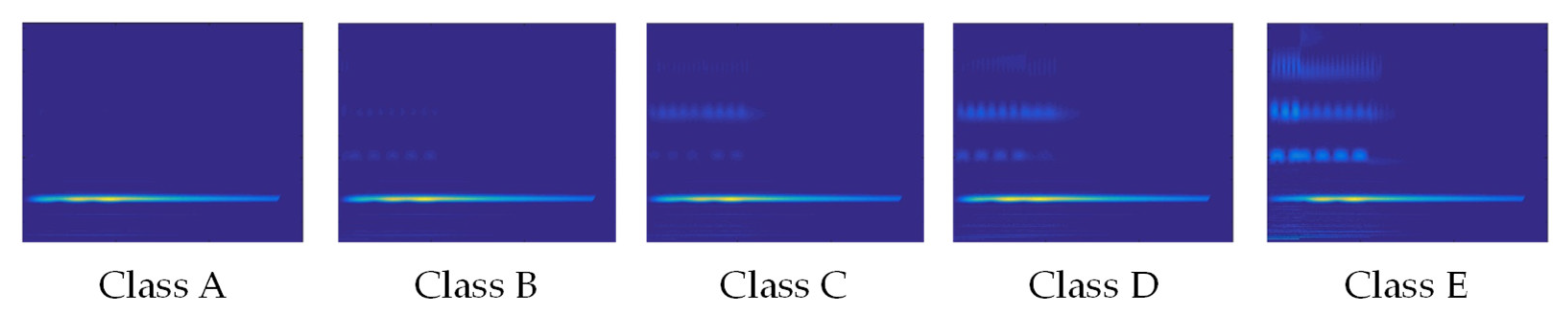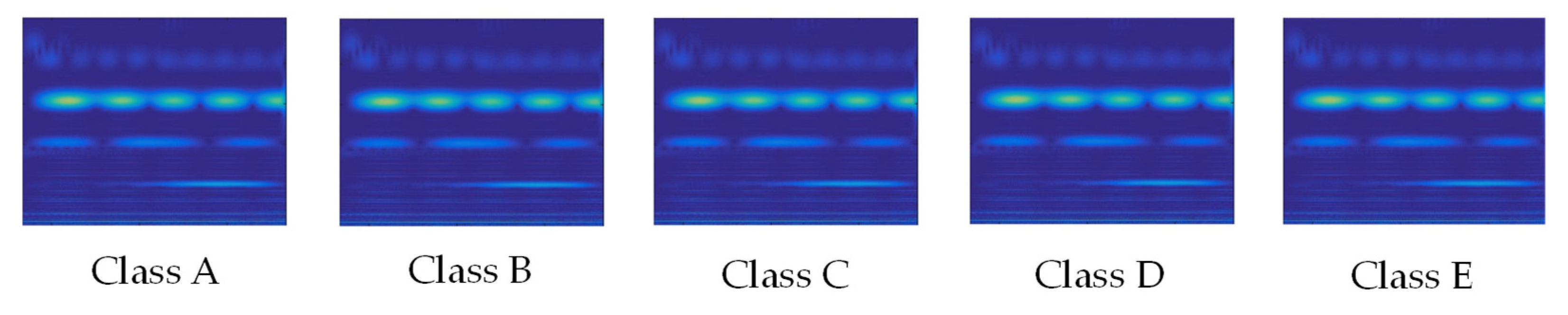Figure 6 and Figure 7 show the displacement sample and acceleration sample images corresponding to five randomly selected vehicle weights, respectively. Visible discrepancy can be observed from those images, which suggests the possibility of accurate identification results. Then, those samples are used as the input of the network model for model training and vehicle weight identification evaluation.

The trained MobileNetV2 model is used to identify vehicle weight information. Because the data characteristics of the target domain are quite different from those of the source domain, the MobileNetV2 model is transferred in the form of fine-tuning. The first 12th Bottlenecks of the MobileNetV2 model are frozen, the rest of the bottlenecks are retrained, and the original 1000-class target classifier are replaced with the 5-class target classifier required for moving load identification in this paper.

In this paper, the stochastic gradient descent algorithm is used to train the model. The learning rate is set to 0.0001. According to the scale of sample data, batch size is set to 64 and epoch is set to 50. Based on Pytorch 2.0, the MobileNetV2 model is trained under the operating system of Windows 10 and CPU of AMD Ryzen 53550H @ 2.10 GHz.

The accuracy and loss curves of the model training to convergence process are shown in Figure 8, and the accuracy and loss at the end of training are shown in

Table 2. Train results of vehicle weights identification after 50 epochs.

Input	Accuracy (%)		Loss
	Training Set	Validation Set	Training Set	Validation Set
Displacement	98.83	98.00	0.0239	0.0714
Velocity	99.62	100.00	0.0105	0.0104
Acceleration	99.43	96.08	0.0275	0.2069

. The vehicle weight is identified by using the test set samples. The identification results and confusion matrix are shown in

Table 3. Identification results of vehicle weights.

Input	Identification Accuracy (%)
Displacement	100.00
Velocity	98.00
Acceleration	96.08

and Figure 8. After careful analysis of Figure 8 and Figure 9 and Table 2 and Table 3, the following conclusions can be drawn:

(1)

The vehicle weight information can be accurately identified from the response samples. For example, it can be seen from Figure 8 that, when the epoch is within 10, the accuracy curve and the loss curve of the training set and verification set input by all the sample change faster. When the epoch is within 10 and 50, the accuracy curve and the loss curve change slowly and gradually tend to be stable. From Table 2, we can see that after the model training completed, the training set accuracy of each input is above 98%, in which the accuracy of the training set of both velocity sample input and acceleration response sample input reached 99%, the accuracy of the validation set of both displacement response sample input and velocity response sample input reached 98%, and the acceleration response sample input also reached 98.83%. It shows that the MobileNetV2 model trained by transfer learning can converge after less iterations. At the same time, the confusion matrix of the test results shows that the proposed method misclassifies only a small number of samples.

(2)

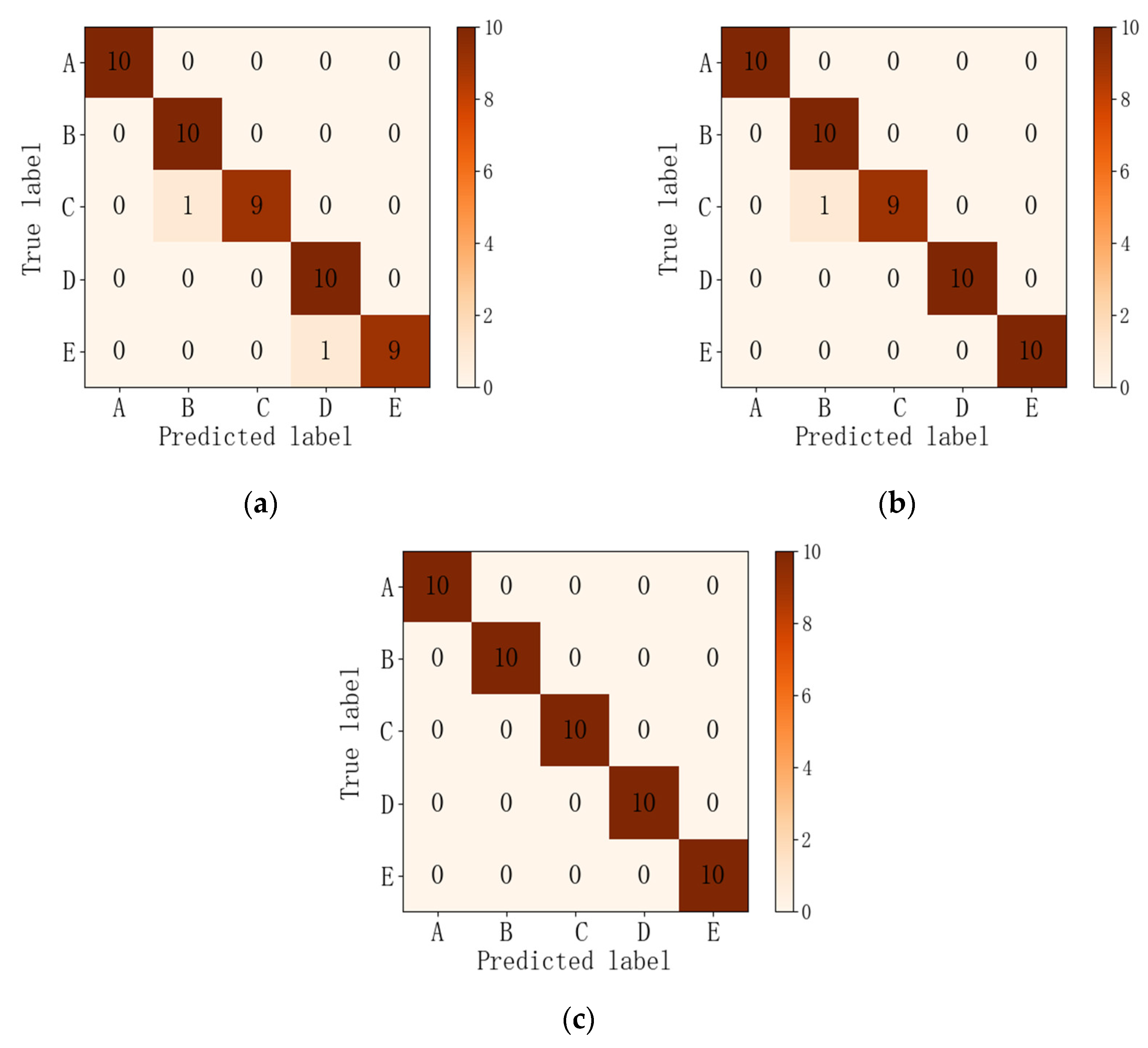
The displacement response sample has the best identification effect on vehicle weight identification tasks. From the test results in Table 3, the identification accuracy using the displacement response is the highest, reaching 100%; the lowest identification accuracy of acceleration response is 96.08%. As can be seen from the confusion matrix in Figure 9, the displacement response profile sample input accurately classifies all test samples, and both acceleration and velocity sample inputs misclassify only a small number of samples. The above analysis shows that the information of vehicle weight is most efficiently identified from displacement responses.

4.3. Vehicle Speed Identification

Acquisition of vehicle speed information is vital for control of vehicle overspeed. Therefore, this paper carries out a vehicle speed identification task to verify the performance of the proposed method in vehicle speed identification. Similar to vehicle weight identification, speed is divided into five grades from slow to fast (A, B, C, D, E). The speed classification table is shown in

Table 4. Classification of vehicle speed.

Class	Vehicle Speed (m/s)	Mean (m/s)
A	0~5	2.5
B	5~10	7.5
C	10~15	12.5
D	15~20	17.5
E	20~25	22.5

.

Similarly, 500 speed samples are randomly generated, including 100 samples per grade. Then, based on the VBI dynamic equations, the responses of each speed sample are obtained in turn under the condition that the vehicle weight is class B, and the unevenness of the road surface is class B. Thus, the sample images are constructed according to the aforementioned strategy to generate a sample library for the vehicle speed identification task. Then, the samples are used as input to the network model for model training and evaluation of vehicle speed identification, respectively.

The accuracy and loss curves of the type training to convergence process are shown in Figure 10. Accuracy and loss at the end of training are shown in

Table 5. Train results of vehicle speed identification after 50 epochs.

Input	Accuracy (%)		Loss
	Training Set	Validation Set	Training Set	Validation Set
Displacement	99.43	96.00	0.0298	0.0236
Velocity	99.61	98.00	0.0662	0.0163
Acceleration	100.00	100.00	0.0148	0.0078

. The identification results and the confusion matrix are shown in

Table 6. Identification results for the vehicle weight.

Input	Identification Accuracy (%)
Displacement	96.00
Velocity	98.00
Acceleration	100.00

and Figure 11. After a detailed analysis of Figure 10 and Figure 11 and Table 5 and Table 6, the following conclusions can be drawn:

(1)

The vehicle speed information can be accurately identified from response samples. For example, as can be seen in Figure 10 and Table 5 that the accuracy and loss of the training set, validation set of the proposed method are gradually stabilized after 10 epochs. The accuracy of each input training set reaches 99% after training, the loss of both the training and validation sets are within 0.03. At the same time, it can be seen from the test results and confusion matrix that this method misclassifies only a small number of samples. Those analysis demonstrate that the method has excellent performance in vehicle weight identification tasks.

(2)

The acceleration response sample has the best identification effect on vehicle speed identification tasks. From the test results in Table 6, the highest identification accuracy of 100% was achieved using acceleration response as input. It can be seen from the confusion matrix of Figure 11 that all test samples are accurately classified by using acceleration response as input, and the information of vehicle speed is most efficiently identified from acceleration responses.

5. Discussion and Analysis

5.1. Comparison of Popular Network Models

To further validate the efficiency of the proposed method, the test results of MobileNetV2 model are compared with those of AlexNet, VGG16, and ResNet. Specifically, the above network models are transferred to identification tasks in the same fine-tuning form as the MobileNetV2 model. The acceleration samples are used as input on vehicle speed identification task, and the displacement samples are used as input on vehicle weight identification task. To compare the computational efficiency of the models, the training time complete 50 epochs, the weight file of model generated after identification of 50 samples in the test set, and the identification time for each model are compared.

The training results for vehicle weights identification task are shown in Figure 12, After 50 epochs, the results of the identification of the test set are shown in

Table 7. Train results of vehicle weight identification of different models after 50 epochs.

Model	Accuracy (%)		Loss		Total Training Time (Min)
	Training Set	Validation Set	Training Set	Validation Set
AlexNet	98.63	94.00	0.0580	0.0837	98
ResNet	99.80	98.00	0.0143	0.0437	95
VGG16	99.80	100.00	0.0137	0.0142	508
MobileNetv2	98.83	98.00	0.0275	0.0714	53

and

Table 8. Identification results of vehicle weight for different models.

Model	Accuracy (%)	Weight File (MB)	Identification Time (s)
AlexNet	98.00	684.31	24.91
ResNet	98.00	134.26	18.78
VGG16	98.00	1573.64	39.76
MobileNetv2	100.00	27.12	11.04

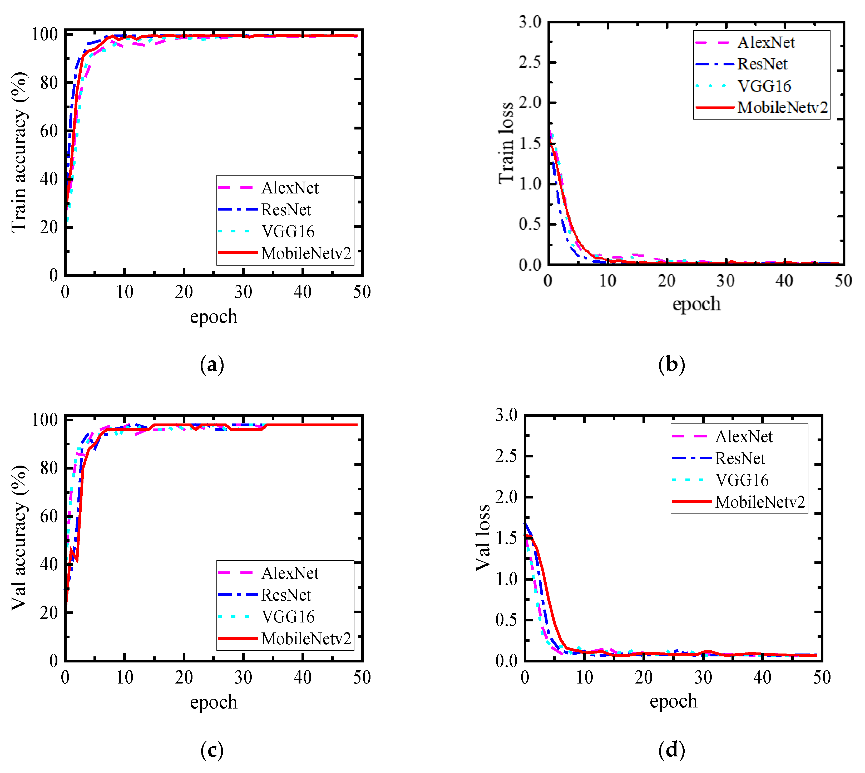
. As can be seen from Figure 12, the MobileNetV2 model and each of the other models have converged after 50 epochs. As can be seen from Table 7, the final accuracy of the training set is above 98% for MobileNetV2 and other models. For the final accuracy of the validation set, VGG16 model has the highest accuracy of 100%, AlexNet has the lowest accuracy of 94%, and MobileNetV2 and ResNet both reach 98%. For training time, MobileNetV2 takes 53 min to train, which is only 10% of VGG16 and 55% of AlexNet and ResNet. In terms of identification speed, MobileNetV2 took 11.04 s to identify 50 test samples, which was only 27.8% of VGG16, 44.3% of AlexNet, and 58.8% of ResNet.

Training results of vehicle speed identification task are shown in Figure 13. The identification results of the test set after 50 epochs are shown in

Table 9. Train results for vehicle speed identification of different models after 50 epochs.

Model	Accuracy (%)		Loss		Total Time (Min)
	Training Set	Validation Set	Training Set	Validation Set
AlexNet	99.23	98.00	0.0251	0.0711	99
ResNet	98.43	98.00	0.0219	0.0751	95
VGG16	98.43	98.00	0.0241	0.0680	508
MobileNetv2	100.00	100.00	0.0148	0.0078	53

and

Table 10. Identification results of vehicle speed for different models.

Model	Accuracy	Weight File (MB)	Identification Time (S)
AlexNet	94.00	684.31	20.40
ResNet	98.00	134.26	19.15
VGG16	100.00	1573.64	38.59
MobileNetv2	100.00	27.12	9.58

. From Figure 13, it can be seen that the MobileNetV2 model and each of the other models have converged after 50 epochs, On the accuracy curves of the training and validation sets, ResNet and MobileNetV2 rise faster and fluctuate less, while AlexNet and VGG16 rise slower and fluctuate more. The accuracy of both the training and validation sets after training is 100% for MobileNetV2 and 98% for all the other three models. Based on the identification results in Table 10, MobileNetV2 and VGG16 have the highest accuracy of 100%, while AlexNet has the lowest accuracy of 94%. The weight file size of MobileNetV2 is only 1.7% of VGG16, 3.9% of AlexNet, and 20% of ResNet, which has obvious advantages. In terms of identification speed, MobileNetV2 takes 9.58S to identify 50 test samples, which is only 24.8% of VGG16, 49.7% of AlexNet, and 50% of ResNet.

In summary, MobileNetV2 outperforms the other three models in both vehicle weight identification and vehicle speed identification tasks, in terms of identification accuracy. At the same time, MobileNetV2 is superior to other models in terms of training time and memory resource occupancy on the premise of ensuring accuracy. Additionally, MobileNetV2 has a major advantage in the speed of identification from the test set. It can be seen that this method has the best performance in terms of identification speed and accuracy, and the short training time and identification time make this method more suitable for practical applications.

5.2. Robustness Analysis

Anti-noise ability is a key basis for judging the practicability of the method. Therefore, this section evaluates its robustness by considering the measurement noise. In this paper, to simulate the actual test environment, the following noise levels of white noise were added to the sample data. In accordance with the implementation steps of the proposed method, the training and testing of the models for the two identification tasks were carried out under different noise levels, with the same transfer process and parameter settings as in the absence of noise; acceleration is used to identify vehicle speed, and displacement is used to identify vehicle weight.

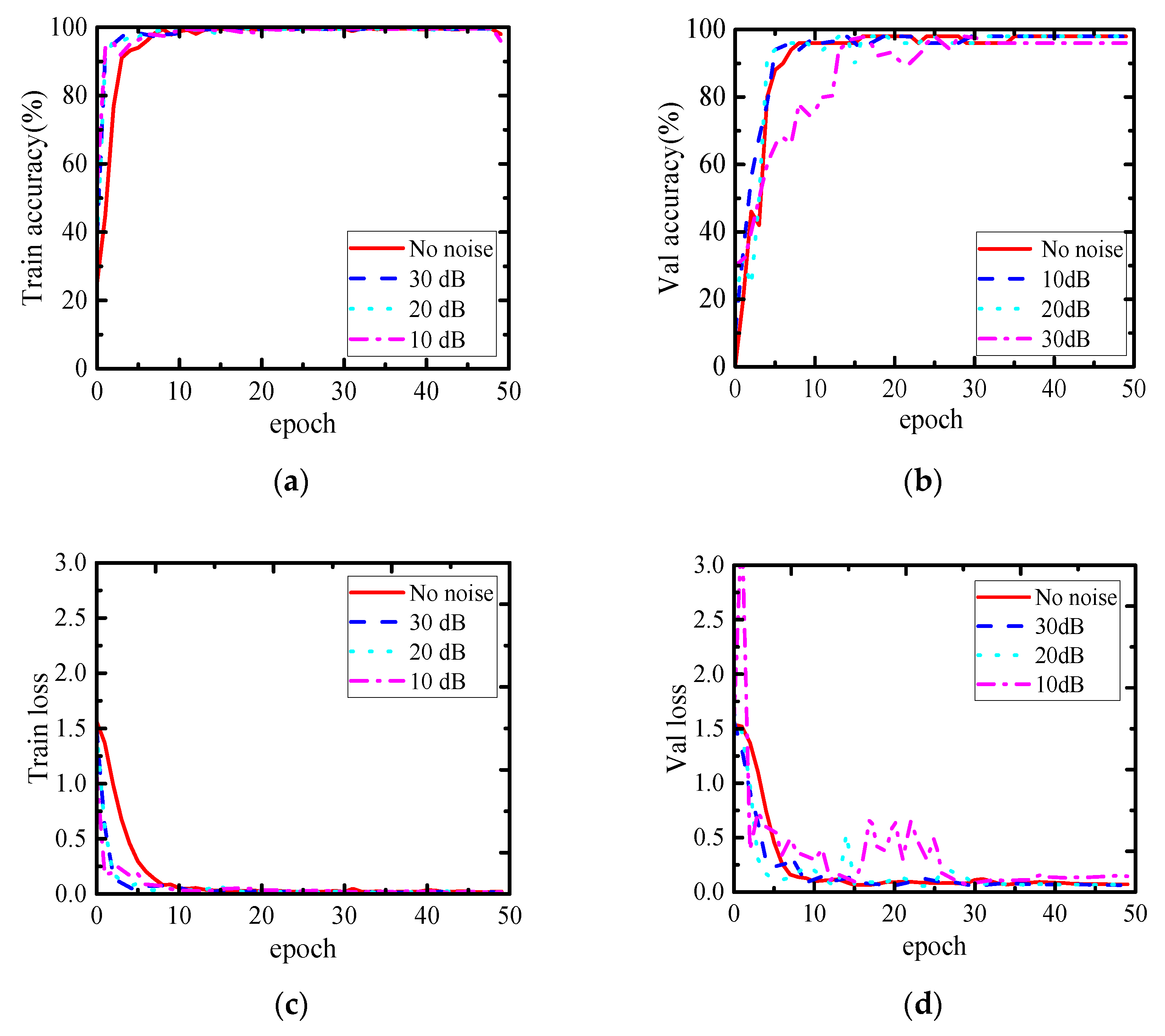
The training results of the vehicle weight identification task are shown in Figure 14. As can be seen from Figure 14, the accuracy and loss curves of the training set do not fluctuate much under different noise levels and the accuracy and loss curves of the validation set fluctuate in the first 20 epochs under 10 dB noise condition, but become smooth at 30 to 50 epochs. The models have converged after 50 epochs for different noise conditions.

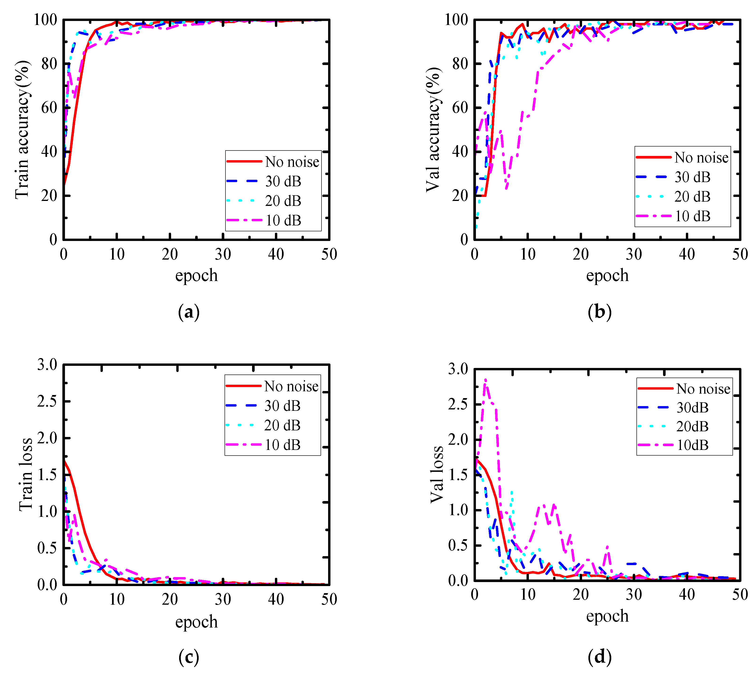
The training results for the vehicle speed identification task are shown in Figure 15. It can be seen that the training set and validation set curves of vehicle speed identification and vehicle weight identification at different noise levels have the same pattern. The accuracy and loss curves of the training set do not fluctuate much. The accuracy and loss curves of the validation set have small fluctuations in the first 20 epochs under 10 dB noise conditions, but become smooth in 30 to 50 epochs.

From the test results in

Table 11. Model Identification results under different noise levels.

Identification Task	No Noise	30 dB	20 dB	10 dB
vehicle weight	100%	98%	98%	98%
vehicle speed	100%	98%	100%	98%

, the identification accuracy of the test set of the vehicle weight identification task decreases and stabilizes at 98%. With the noise level increases, identification accuracy of test set in vehicle speed identification decreased slightly. The accuracy at 30 dB and 10 dB was 98%, and the accuracy of 20 dB was still 100%. It shows that there is no obvious downward trend in the accuracy of model test, and there is only a slight fluctuation. It can be concluded that the proposed method presents excellent, strong robustness.

6. Conclusions

This paper presents a moving load identification method based on MobileNetV2 and transfer learning. The performance of the proposed method is verified by the numerical simulation and parameter analysis. The main conclusions were obtained as follows:

(1)

Vehicle load information can be accurately separated from the responses of the established VBI dynamic model by the proposed method. The displacement response is the most effective model input on vehicle weight identification task, with an identification accuracy of 100%. The acceleration response is the most effective input of model for vehicle speed identification task, with 100% identification accuracy.

(2)

The proposed method has higher identification efficiency. Lightweight convolutional neural networks and transfer learning strategies can improve identification efficiency. Compared to VGG16, AlexNet, and ResNet, the training time of MobileNetV2 is reduced by more than 50%, and the identification speed of MobileNetV2 is increased by more than 42.2% on vehicle weight identification and more than 50% on vehicle speed identification. In addition, the storage occupancy of MobileNetV2 is only 1.7% of VGG16, 3.9% of AlexNet, and 20% of ResNet.

(3)

The proposed method has excellent robustness. The robustness analysis shows that the method can still maintain excellent identification ability when encountering a higher noise level. At 10 dB noise level, the identification accuracy of vehicle speed and vehicle weight still reached 98%.

Although this method has achieved satisfactory identification results on the established numerical scenarios, it cannot directly address cases where vehicles are distributed in multiple lanes and drive in opposite direction. In addition, for vehicles with multiple axles, it is difficult to identify the axle weight of each wheel. Therefore, the future work will focus on further improving the practicality of the proposed method.

References

1. Tang, Q.Z.; Zhou, J.T.; Xin, J.Z. Fast identification of random loads using the transmissibility of power spectral density and improved adaptive multiplicative regularization. J. Sound Vib. 2022, 534, 117033. [Google Scholar] [CrossRef]
2. Xin, J.Z.; Jiang, Y.; Zhou, J.T. Bridge deformation prediction based on SHM data using improved VMD and conditional KDE. Eng. Struct. 2022, 261, 114285. [Google Scholar] [CrossRef]
3. Zhang, H.; Li, H.X.; Zhou, J.T. A multi-dimensional evaluation of wire breakage in bridge cable based on self-magnetic flux leakage signals. J. Magn. Magn. Mater. 2023, 566, 170321. [Google Scholar] [CrossRef]
4. Jiang, Y.; Hui, Y.; Wang, Y. A novel eigenvalue-based iterative simulation method for multi-dimensional homogeneous non-Gaussian stochastic vector fields. Struct. Saf. 2023, 100, 102290. [Google Scholar] [CrossRef]
5. Li, S.J.; Xin, J.Z.; Jiang, Y. Temperature-induced deflection separation based on bridge deflection data using the TVFEMD-PE-KLD method. J. Civ. Struct. Health 2023. [Google Scholar] [CrossRef]
6. Zhu, X.Q.; Law. S.S, Recent developments in inverse problems of vehicle–bridge interaction dynamics. J. Civ. Struct. Health 2016, 6, 107–128. [Google Scholar] [CrossRef]
7. Zhang, H.; Zhou, Y.; Quan, L. Identification of a moving mass on a beam bridge using piezoelectric sensor arrays. J. Sound Vib. 2021, 491, 115754. [Google Scholar] [CrossRef]
8. Yu, Y.; Cai, C.S.; Deng, L. State-of-the-art review on bridge weigh-in motion technology. Adv. Struct. Eng. 2016, 19, 1514–1530. [Google Scholar] [CrossRef]
9. Lee, S. An advanced coupled genetic algorithm for identifying unknown moving loads on bridge decks. Math. Probl. Eng. 2014, 2014, 462341. [Google Scholar] [CrossRef] [Green Version]
10. Wang, Y.; Qu, W. Experimental study on moving train loads identification from bridge responses. Adv. Mater. Res. 2010, 143–144, 32–37. [Google Scholar] [CrossRef]
11. Pan. C.D.; Yu, L. Moving force identification based on firefly algorithm. AMR 2014, 919–921, 329–333. [Google Scholar] [CrossRef]
12. Liu, H.; Yu, L. Moving force identification based on particle swarm optimization. In Proceedings of the 2016 12th International Conference on Natural Computation, Fuzzy Systems and Knowledge Discovery (ICNC-FSKD), Changsha, China, 13–15 August 2016; pp. 825–829. [Google Scholar] [CrossRef]
13. Vosoughi, A.R.; Anjabin, N. Dynamic moving load identification of laminated composite beams using a hybrid FE-TMDQ-GAs method. Inverse Probl. Sci. Eng. 2017, 25, 1639–1652. [Google Scholar] [CrossRef]
14. Liu, R.; Dobriban, E.; Hou, Z. Dynamic load identification for mechanical systems: A review. Arch. Comput. Methods Eng. 2022, 29, 831–863. [Google Scholar] [CrossRef]
15. Wang, C.; Ansari, F.; Wu, B.; Li, S.; Morgese, M.; Zhou, J. LSTM approach for condition assessment of suspension bridges based on time-series deflection and temperature data. Adv. Struct. Eng. 2022, 25, 3450–3463. [Google Scholar] [CrossRef]
16. Yang, H.; Yan, W.; He, H. Parameters identification of moving load using ANN and dynamic strain. Shock Vib. 2016, 2016, 8249851. [Google Scholar] [CrossRef] [Green Version]
17. Zhou, Y.; Pei, Y.; Zhou, S. Novel methodology for identifying the weight of moving vehicles on bridges using structural response pattern extraction and deep learning algorithms. Measurement 2021, 168, 108384. [Google Scholar] [CrossRef]
18. Chen, T.; Guo, L.; Duan, A. A feature learning-based method for impact load reconstruction and localization of the plate-rib assembled structure. Struct. Health Monit. 2022, 21, 1590–1607. [Google Scholar] [CrossRef]
19. Zhang, H.; Zhou, Y. AI-based modeling and data-driven identification of moving load on continuous beams. Fundam. Res. 2022, in press. [Google Scholar] [CrossRef]
20. Sandler, M.; Howard, A.; Zhu, M.; Zhmoginov, A.; Chen, L.C. MobileNetV2: Inverted residuals and linear bottlenecks. In Proceedings of the 2018 IEEE/CVF Conference on Computer Vision and Pattern Recognition, Salt Lake City, UT, USA, 18–23 June 2018; pp. 4510–4520. [Google Scholar] [CrossRef] [Green Version]
21. Pourzeynali, S.; Zhu, X.; Zadeh, A.G. Comprehensive study of moving load identification on bridge structures using the explicit form of Newmark-β method: Numerical and Experimental Studies. Remote Sens. 2021, 13, 2291. [Google Scholar] [CrossRef]
22. Agostinacchio, M.; Ciampa, D.; Olita, S. The vibrations induced by surface irregularities in road pavements-a Matlab approach. Eur. Transp. Res. Rev. 2013, 6, 267–275. [Google Scholar] [CrossRef] [Green Version]
23. Tang, Q.Z.; Zhou, J.T.; Xin, J.Z. Novel identification technique of moving loads using the random response power spectral density and deep transfer learning. Measurement 2022, 195, 111120. [Google Scholar] [CrossRef]
24. Lecun, Y.; Bottou, L.; Bengio, Y. Gradient-based learning applied to document recognition. Proc. IEEE 1998, 86, 2278–2324. [Google Scholar] [CrossRef] [Green Version]
25. Krizhevsky, A.; Sutskever, I.; Hinton, G. Imagenet classification with deep convolutional neural networks. Commun. ACM 2017, 60, 84–90. Available online: https://dl.acm.org/doi/10.1145/3065386 (accessed on 3 January 2023). [CrossRef] [Green Version]
26. Simonyan, K.; Zisserman, A. Very deep convolutional networks for large-scale image recognition. arXiv 2014, arXiv:1409.1556. [Google Scholar] [CrossRef]
27. Szegedy, C.; Liu, W.; Jia, Y. Going deeper with convolutions. In Proceedings of the 2015 IEEE Conference on Computer Vision and Pattern Recognition (CVPR), Boston, MA, USA, 7–12 June 2015; pp. 1–9. [Google Scholar] [CrossRef] [Green Version]
28. He, K.; Zhang, X.; Ren, S.; Sun, J. Deep residual learning for image recognition. In Proceedings of the 2016 IEEE Conference on Computer Vision and Pattern Recognition (CVPR), Las Vegas, NV, USA, 27–30 June 2016; pp. 770–778. [Google Scholar] [CrossRef] [Green Version]
29. Huang, G.; Liu, Z.; Laurens, V.; Weinberger, K.Q. Densely connected convolutional networks. In Proceedings of the 2017 IEEE Conference on Computer Vision and Pattern Recognition (CVPR), Honolulu, HI, USA, 21–26 July 2017; pp. 2261–2269. [Google Scholar] [CrossRef] [Green Version]
30. Howard, A.; Zhu, M.; Chen, B. MobileNets: Efficient convolutional neural networks for mobile vision applications. arXiv 2017, arXiv:1704.04861. [Google Scholar] [CrossRef]
31. Zhuo, D.; Cao, H. Damage identification of bolt connections base on wavelet time-frequency diagrams and lightweight convolution neural networks. Eng. Mech. 2021, 38, 228–238. [Google Scholar] [CrossRef]
32. Li, Y.T.; Huang, H.S.; Xie, Q.S. Research on a surface defect detection algorithm based on MobileNet-SSD. Appl. Sci. 2018, 8, 1678. [Google Scholar] [CrossRef] [Green Version]
33. Pan, H.; Pang, Z.; Wang, Y.; Chen, L. A New Image recognition and classification method combining transfer learning algorithm and MobileNet model for welding defects. IEEE Access 2020, 8, 119951–119960. [Google Scholar] [CrossRef]
34. Srinivasu, P.N.; Sivasai, J.G.; Ijaz, M.F. Classification of skin disease using deep learning neural networks with MobileNet V2 and LSTM. Sensors 2021, 21, 2852. [Google Scholar] [CrossRef]
35. Pan, S.J.; Yang, Q. A survey on transfer learning. IEEE Trans. Knowl. Data Eng. 2010, 10, 1345–1359. [Google Scholar] [CrossRef]
36. Liang, P.F.; Deng, C.; Wu, J. Intelligent fault diagnosis of rotating achinery via wavelet transform, generative adversarial nets and convolutional neural network. Measurement 2020, 159, 107768. [Google Scholar] [CrossRef]
37. Yang, J.; Chen, R.; Zhang, Z. Experimental study on the ultimate bearing capacity of damaged RC arches strengthened with ultra-high performance concrete. Eng. Struct. 2023, 279, 115611. [Google Scholar] [CrossRef]
38. Tan, H.; Qian, D.; Xu, Y.; Yuan, M.; Zhao, H. Analysis of vertical temperature gradients and their effects on hybrid girder cable-stayed bridges. Sustainability 2023, 15, 1053. [Google Scholar] [CrossRef]
39. Zeng, Y.; He, H.; Qu, Y.; Sun, X.; Tan, H.; Zhou, J. Numerical simulation of fatigue cracking of diaphragm notch in orthotropic steel deck model. Materials 2023, 16, 67. [Google Scholar] [CrossRef] [PubMed]
Figure 1. The VBI system.
Buildings 13 00572 g001
Figure 2. Convolution process of MobileNetV2.
Buildings 13 00572 g002
Figure 3. Illustration of transfer learning strategy process.
Buildings 13 00572 g003
Figure 4. Overview of the proposed method.
Buildings 13 00572 g004
Figure 5. Vehicle-bridge system with single degree of freedom.
Buildings 13 00572 g005
Figure 6. Displacement sample images of five randomly selected vehicle weights.
Buildings 13 00572 g006
Figure 7. Acceleration sample images of five randomly selected vehicle weights.
Buildings 13 00572 g007
Figure 8. Results of vehicle weights identification: (a) Training accuracy curves of response samples; (b) Training loss curves of the response samples; (c) Validation accuracy curves of the response samples; (d) Validation loss curves of response samples.
Buildings 13 00572 g008
Figure 9. Confusion matrix for vehicle weight identification results: (a) Test results of acceleration samples; (b) Test results of speed sample; (c) Test results of displacement sample.
Buildings 13 00572 g009
Figure 10. Results of vehicle speed identification: (a) Training accuracy curves of response samples; (b) Training loss curves of the response samples; (c) Validation accuracy curves of the response samples; (d) Validation loss curves of response samples.
Buildings 13 00572 g010
Figure 11. Confusion matrix for vehicle speed identification results: (a) Test results of acceleration samples; (b) Test results of speed sample; (c) Test results of displacement sample.
Buildings 13 00572 g011
Figure 12. Results of vehicle weights identification of different models: (a) Training accuracy curves of response samples; (b) Training loss curves of the response samples; (c) Validation accuracy curves of the response samples; (d) Validation loss curves of response samples.
Buildings 13 00572 g012
Figure 13. Results of vehicle speed identification of different models: (a) Training accuracy curves of response samples; (b) Training loss curves of the response samples; (c) Validation accuracy curves of the response samples; (d) Validation loss curves of response samples.
Buildings 13 00572 g013
Figure 14. Results of vehicle weights identification under different noise levels: (a) Training accuracy curves of response samples; (b) Validation accuracy curves of the response samples; (c) Training loss curves of the response samples; (d) Validation loss curves of response samples.
Buildings 13 00572 g014
Figure 15. Results of vehicle speed identification under different noise levels: (a) Training accuracy curves of response samples; (b) Validation accuracy curves of the response samples; (c) Training loss curves of the response samples; (d) Validation loss curves of response samples.
Buildings 13 00572 g015