
Prediction of the Shear Resistance of Headed Studs Embedded in Precast Steel–Concrete Structures Based on an Interpretable Machine Learning Method

Abstract
:1. Introduction
2. Physics-Based Equations
2.1. Eurocode-4
2.2. Chinese GB50017–2017 Code
2.3. AASHTO LRFD Bridge Design Codes
3. Data
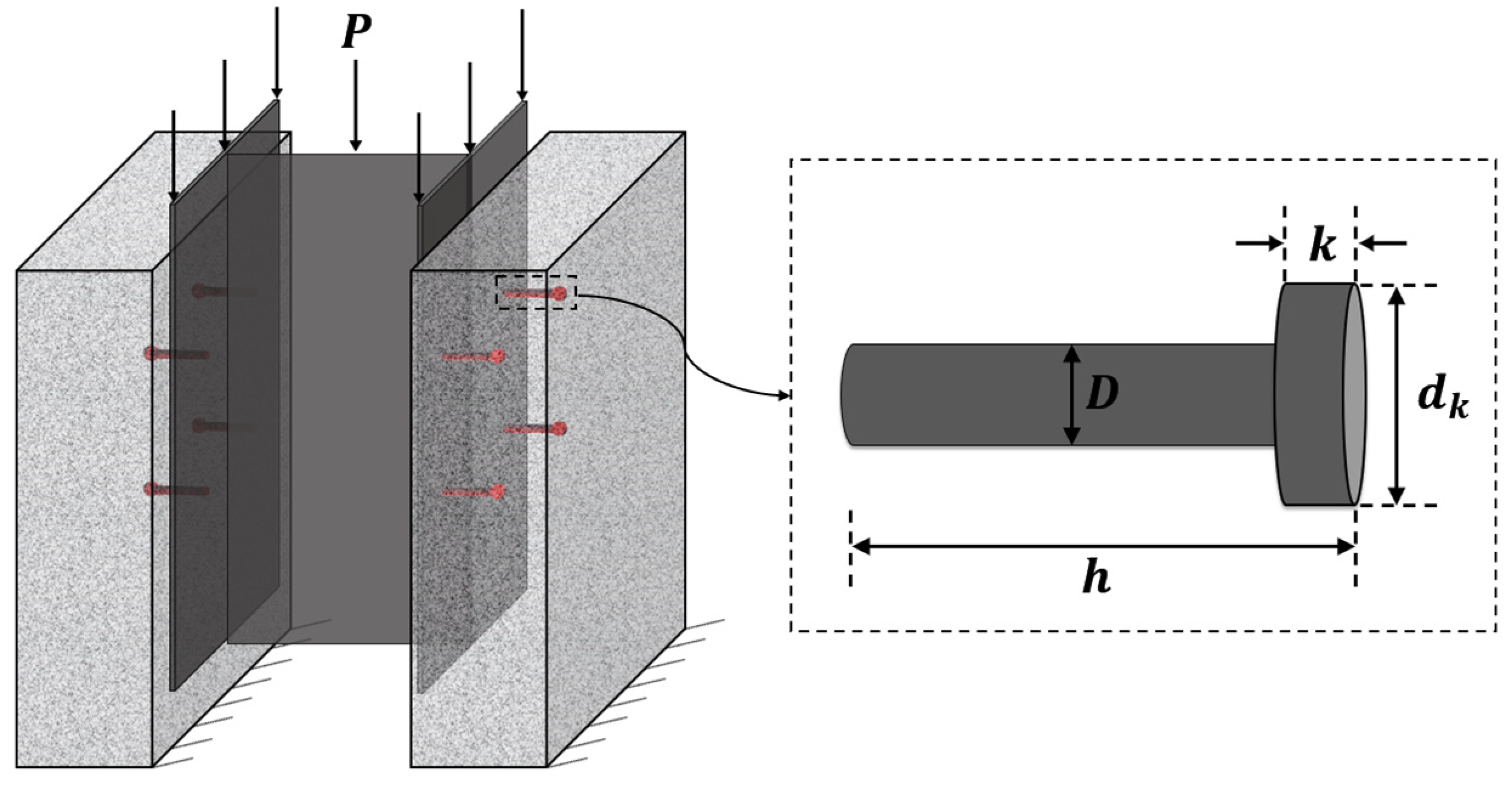
3.1. Dataset of Headed Studs Embedded in Concrete Push-Out Test Specimens
- The test is a push-out test and uses two symmetrical concrete slabs;
- The connectors are headed studs, so specimens with bolts were discarded;
- The loading modes are monotonic loading and cyclic loading, which is closer to the actual engineering loading;
- The materials of the concrete slab are not limited to ordinary concrete, but UHPC and HPC are also collected.
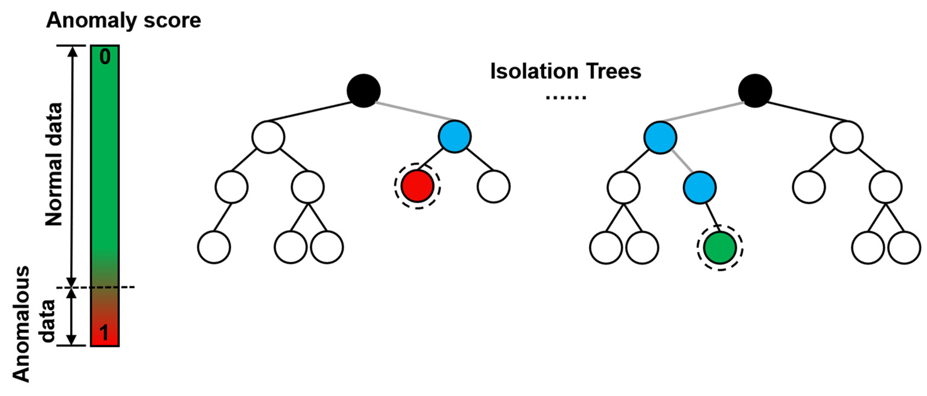
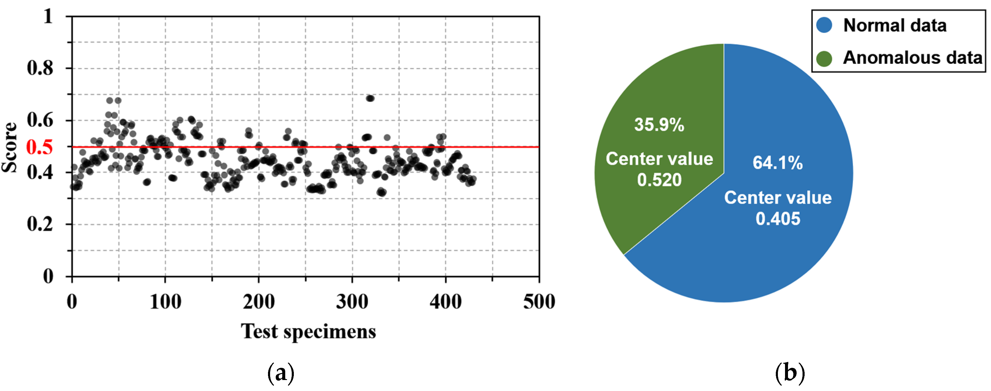
3.2. Anomaly Detection
- 5.
- If instances return a score very close to 1, then they are highly likely to be anomalies;
- 6.
- If instances have a score much smaller than 0.5, then they are quite safe to be regarded as normal instances;
- 7.
- If all the instances return a score ≈ of 0.5, then the entire sample does not really have any distinct anomaly.
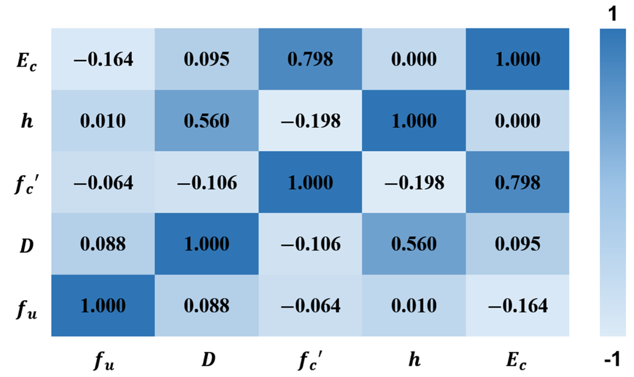
3.3. Pearson Correlation Coefficient Analysis
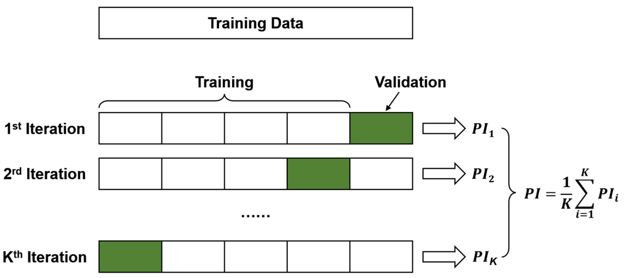
3.4. Performance Metrics
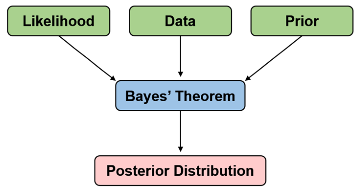
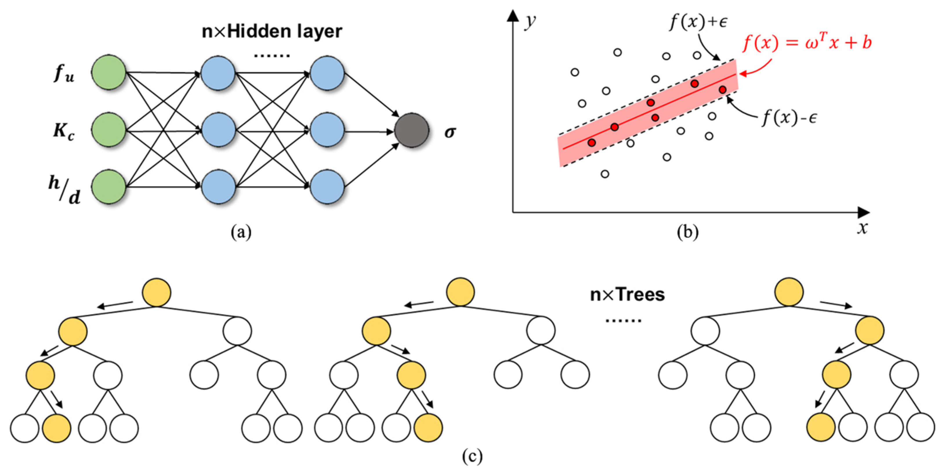
4. ML Algorithms
5. Results and Discussion
6. Visualization and Interpretation of GBDT Model
7. Conclusions
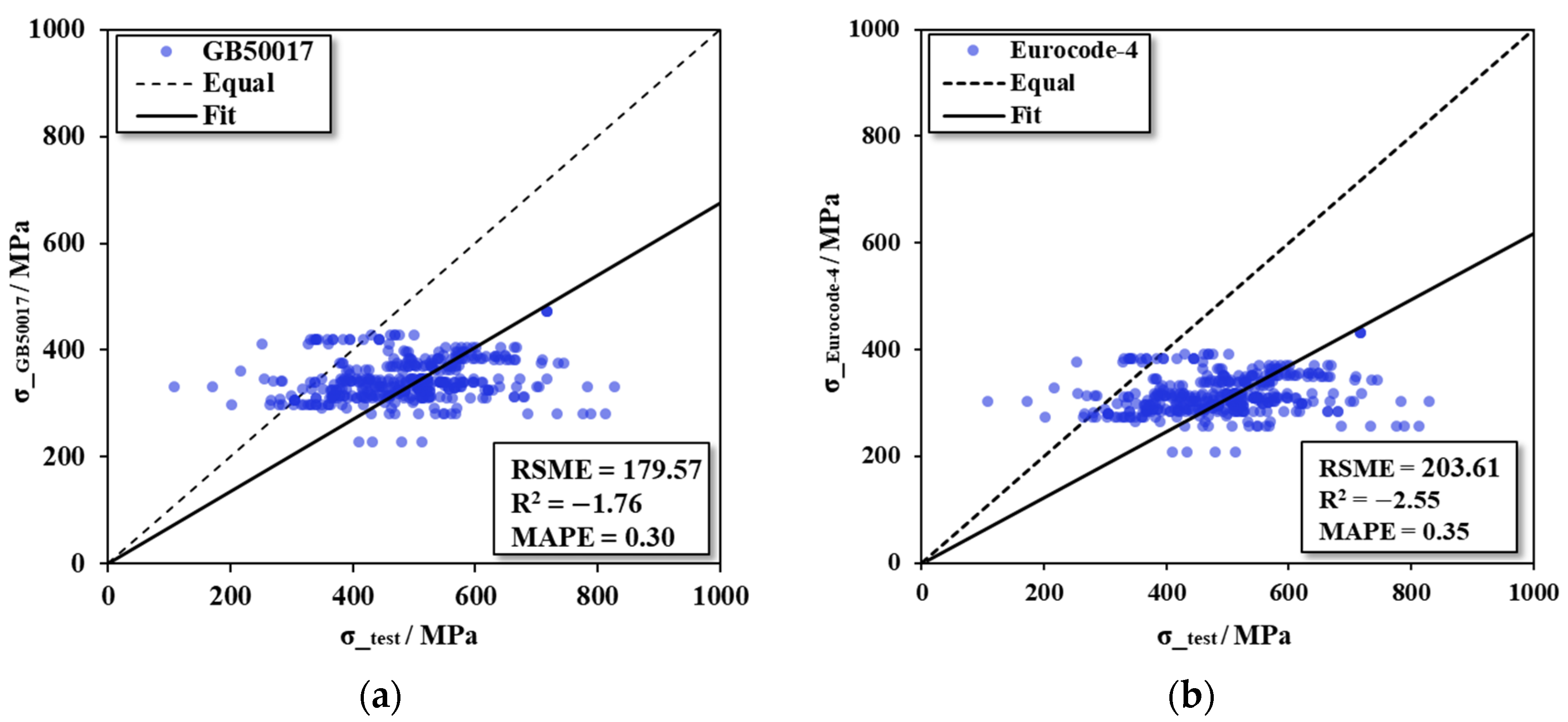
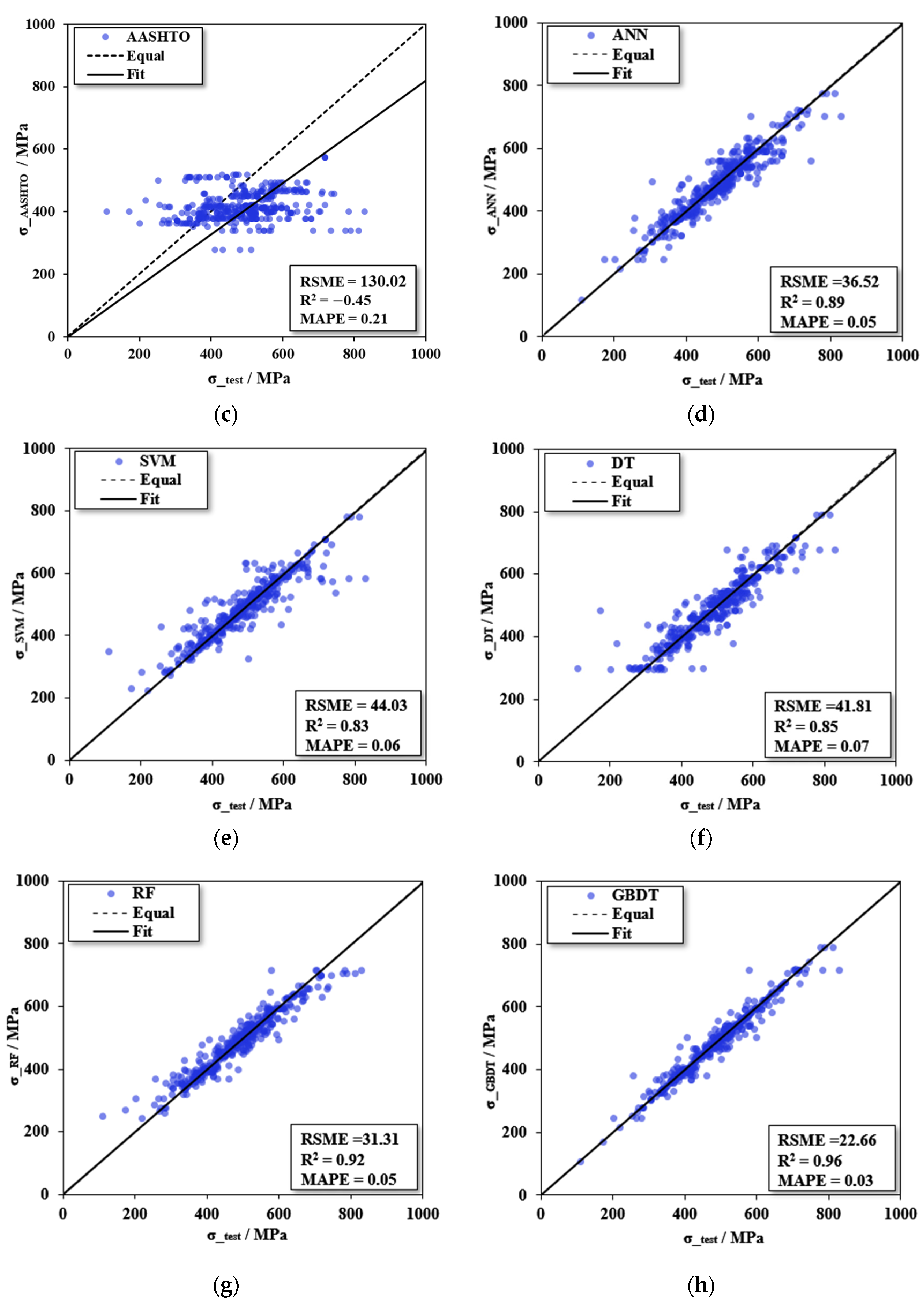
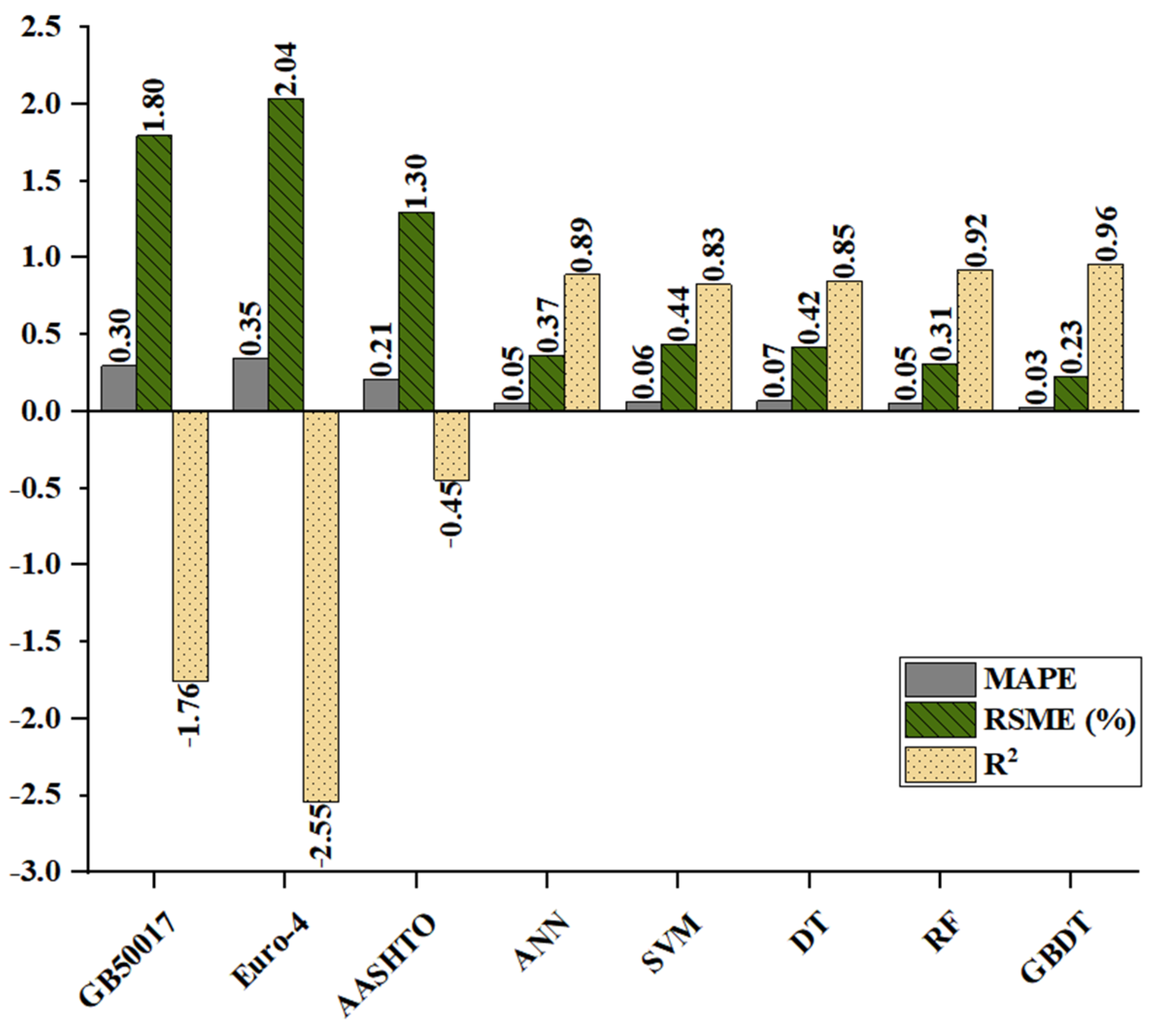
- The values of the equations from design codes of various countries were all negative when predicting datasets, including HPC and UHPC, which means these equations cannot be used for headed studs in HPC and UHPC.
- The prediction accuracy of ML models was much higher than the international design codes. The gradient boosting decision tree (GBDT) model had the overall highest accuracy and was compared with AASHTO, which had the highest accuracy among the three design codes. The values of and of the GBDT model were around 80% lower than that of the AASHTO equation.
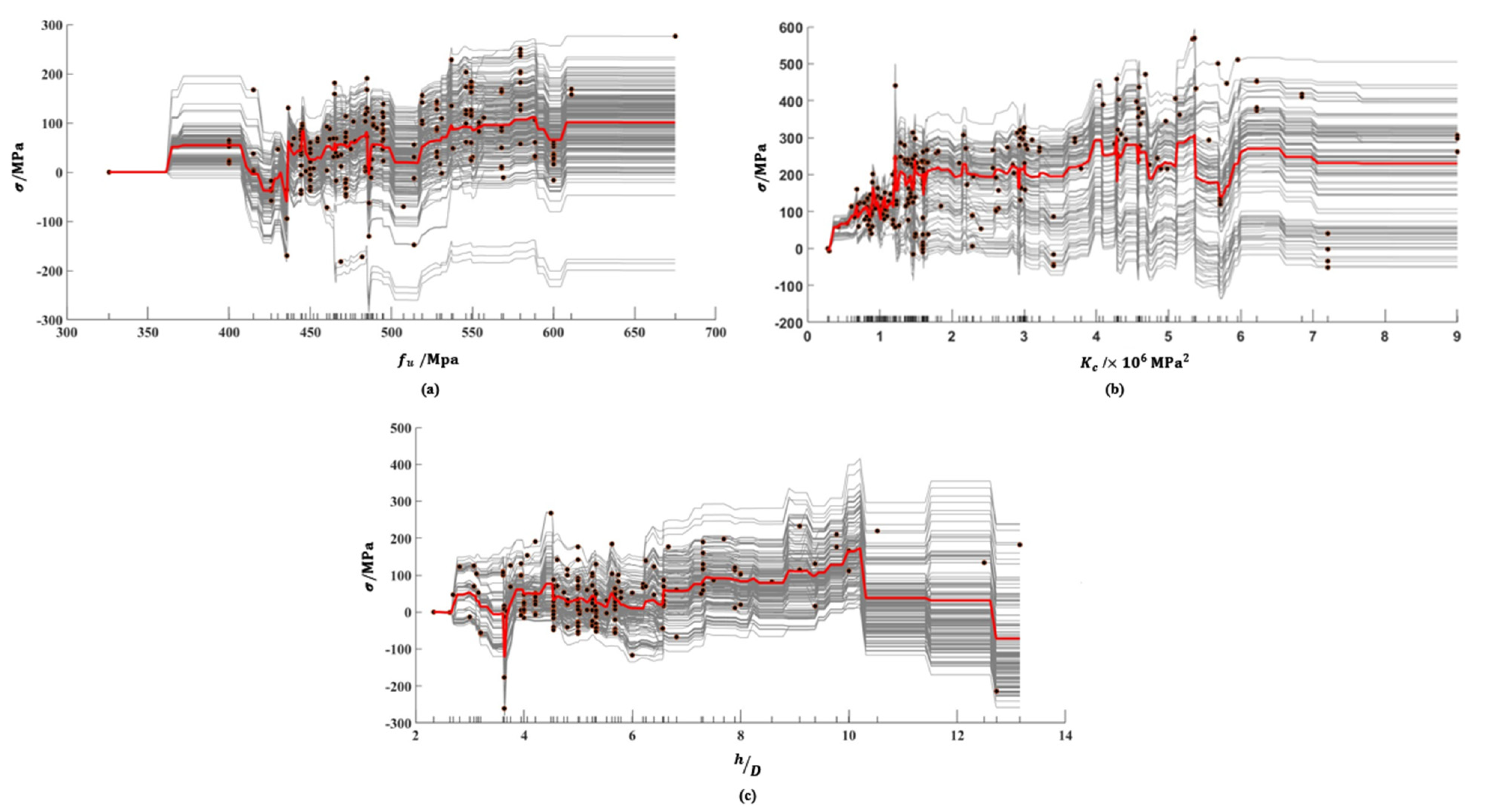
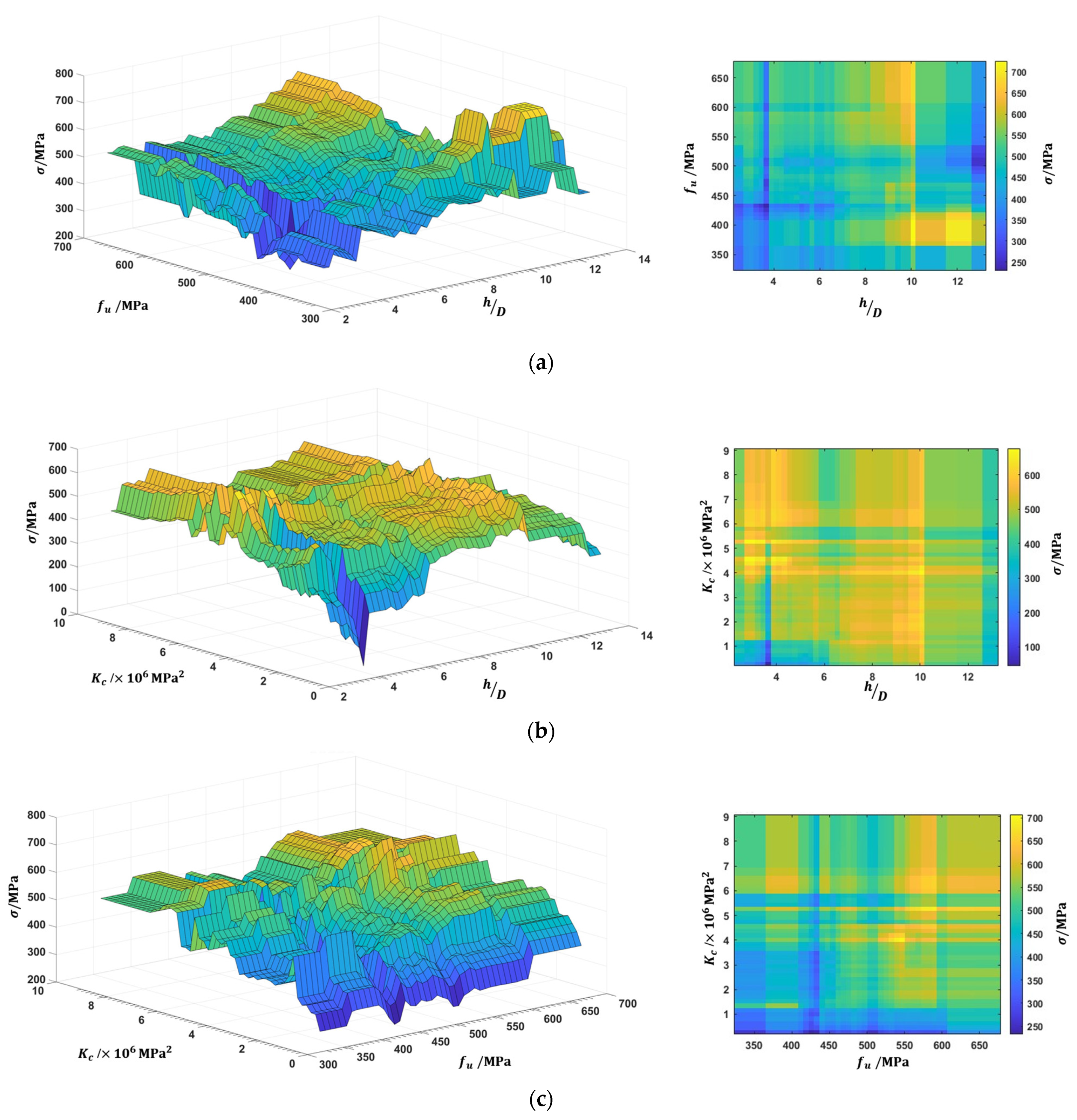
- The visualization and interpretability analysis of the GBDT model showed that the length-to-diameter ratio of the stud had a substantial influence on the shear resistance of headed studs, which may be related to the effect of the length on the pull-out effect of the stud.
- The length-to-diameter ratio of the stud was suggested to be taken into account in the equations of future design codes, and there may be an upper limit on the positive effect of material properties on the shear resistance of headed studs, which requires future supplementation of high-strength material tests to determine.
Author Contributions
Funding
Data Availability Statement
Conflicts of Interest
References
- Nie, J.; Cai, C.S. Steel-concrete composite beams considering shear slip effects. J. Struct. Eng. 2003, 129, 495–506. [Google Scholar] [CrossRef]
- Nie, J.; Wang, J.; Gou, S.; Zhu, Y.; Fan, J. Technological development and engineering applications of novel steel-concrete composite structures. Front. Struct. Civ. Eng. 2019, 13, 1–14. [Google Scholar] [CrossRef]
- Ashraf, M.; Hasan, M.J.; Al-Deen, S. Semi-rigid behaviour of stainless steel beam-to-column bolted connections. Sustain. Struct. 2021, 1, 000002. [Google Scholar] [CrossRef]
- Qi, J.; Hu, Y.; Wang, J.; Li, W. Behavior and strength of headed stud shear connectors in ultra-high performance concrete of composite bridges. Front. Struct. Civ. Eng. 2019, 13, 1138–1149. [Google Scholar] [CrossRef]
- Johnson, R.P. Composite Structures of Steel and Concrete: Beams, Slabs, Columns and Frames for Buildings; John Wiley Sons: New York, NY, USA, 2018; 288p. [Google Scholar]
- Viest, I.M. Investigation of stud shear connectors for composite concrete and steel T.-beams. ACI J. 1956, 27, 875–981. [Google Scholar]
- Ollgaard, J.G.; Slutter, R.G.; Fisher, J.W. Shear strength of stud connectors in lightweight and normal weight concrete. AISC Eng. J. 1971, 71-10, 55-34. [Google Scholar]
- Civjan, S.A.; Singh, P. Behavior of shear studs subjected to fully reversed cyclic loading. J. Struct. Eng. 2003, 129, 1466–1474. [Google Scholar] [CrossRef]
- Eurocode-4; Design of Composite Steel and Concrete Structures. European Committee for Standardization: Brussels, Belgium, 2004.
- AASHTO. AASHTO LRFD Bridge Design Codes; American Association of State Highway and Transportation Officials: Washington, DC, USA, 2012; p. 20001.
- GB50017–2017; Code for Design of Steel Structures. Ministry of Housing and Urban-Rural Development of China: Beijing, China, 2017. (In Chinese)
- Model Code. Joint Committee IASBSE/CEB/FIP/ECCS Composite Structures (Model Code); Construction Press: London, UK, 1981. [Google Scholar]
- Lee, P.G.; Shim, C.S.; Chang, S.P. Static and fatigue behavior of large stud shear connectors for steel–concrete composite bridges. J. Construct. Steel Res. 2005, 61, 1270–1285. [Google Scholar] [CrossRef]
- Hicks, S.J. Design shear resistance of headed studs embedded in solid slabs and encasements. J. Construct. Steel Res. 2017, 139, 339–352. [Google Scholar] [CrossRef]
- Oehlers, D.J.; Foley, L. The fatigue strength of stud shear connections in composite beams. Proc. Inst. Civ. Eng. 1985, 79, 349–364. [Google Scholar] [CrossRef]
- Lin, Z.F.; Liu, Y.Q. Experimental study on shear behavior of large stud connectors. J. Tongji 2015, 43, 1788–1793. (In Chinese) [Google Scholar]
- Duan, M.; Zou, X.; Bao, Y.; Li, G.; Chen, Y.; Li, Z. Experimental investigation of headed studs in steel-ultra-high performance concrete (UHPC) composite sections. Eng. Struct. 2022, 270, 114875. [Google Scholar] [CrossRef]
- Soleimani-Babakamali, M.H.; Esteghamati, M.Z. Estimating seismic demand models of a building inventory from nonlinear static analysis using deep learning methods. Eng. Struct. 2022, 266, 114576. [Google Scholar] [CrossRef]
- Esteghamati, M.Z.; Flint, M.M. Developing data-driven surrogate models for holistic performance-based assessment of mid-rise RC frame buildings at early design. Eng. Struct. 2021, 245, 112971. [Google Scholar] [CrossRef]
- Al-Bashiti, M.K.; Naser, M.Z. Machine learning for wildfire classification: Exploring blackbox, eXplainable, symbolic, and SMOTE methods. Nat. Hazard Res. 2022, 2, 154–165. [Google Scholar] [CrossRef]
- Avci-Karatas, C. Application of machine learning in prediction of shear capacity of headed steel studs in steel-concrete composite structures. Int. J. Steel Struct. 2022, 22, 539–556. [Google Scholar] [CrossRef]
- Cao, Y.; Wakil, K.; Alyousef, R.; Jermsittiparsert, K.; Ho, L.; Alabduljabbar, H.; Alaskar, A.; Alrshoudi, F.; Mohamed, A.M. Application of extreme learning machine in behavior of beam to column connections. Structures 2020, 25, 861–867. [Google Scholar] [CrossRef]
- Gholampour, A.; Mansouri, I.; Kisi, O.; Ozbakkaloglu, T. Evaluation of mechanical properties of concretes containing coarse recycled concrete aggregates using multivariate adaptive regression splines (MARS), M5 model tree (M5Tree), and least squares support vector regression (LSSVR) models. Neural Comput. Appl. 2020, 32, 295–308. [Google Scholar] [CrossRef]
- Huang, C.; Huang, S. Predicting capacity model and seismic fragility estimation for RC bridge based on artificial neural network. Structures 2020, 27, 1930–1939. [Google Scholar] [CrossRef]
- Wang, X.; Liu, H.; Liu, Y. Auto-tuning deep forest for shear stiffness prediction of headed stud connectors. Structures 2022, 43, 1463–1477. [Google Scholar] [CrossRef]
- Mahjoubi, S.; Meng, W.; Bao, Y. Logic-guided neural network for predicting steel-concrete interfacial behaviors. Exp. Syst. Appl. 2022, 198, 116820. [Google Scholar] [CrossRef]
- Zhou, Y.; Zheng, S.; Huang, Z.; Sui, L.; Chen, Y. Explicit neural network model for predicting FRP-concrete interfacial bond strength based on a large dataset. Compos. Struct. 2020, 240, 111998. [Google Scholar] [CrossRef]
- Zhang, F.; Wang, C.; Liu, J.; Zou, X.; Sneed, L.H.; Bao, Y.; Wang, L. Prediction of FRP-concrete interfacial bond strength based on machine learning. Eng. Struct. 2023, 274, 115156. [Google Scholar] [CrossRef]
- Lee, S.; Lee, C. Prediction of shear strength of FRP-reinforced concrete flexural members without stirrups using artificial neural networks. Eng. Struct. 2014, 61, 99–112. [Google Scholar] [CrossRef]
- Vinuesa, R.; Brunton, S.L. Enhancing computational fluid dynamics with machine learning. Nat. Comput. Sci. 2022, 2, 358–366. [Google Scholar] [CrossRef]
- Tran, V.Q.; Dang, V.Q.; Ho, L.S. Evaluating compressive strength of concrete made with recycled concrete aggregates using machine learning approach. Construct. Build. Mater. 2022, 323, 126578. [Google Scholar] [CrossRef]
- Yuan, X.; Tian, Y.; Ahmad, W.; Ahmad, A.; Usanova, K.I.; Mohamed, A.M.; Khallaf, R. Machine Learning Prediction Models to Evaluate the Strength of Recycled Aggregate Concrete. Materials 2022, 15, 2823. [Google Scholar] [CrossRef] [PubMed]
- Asteris, P.G.; Skentou, A.D.; Bardhan, A.; Samui, P.; Pilakoutas, K. Predicting concrete compressive strength using hybrid ensembling of surrogate machine learning models. Cem. Concr. Res. 2021, 145, 106449. [Google Scholar] [CrossRef]
- Cakiroglu, C.; Islam, K.; Bekdaş, G.; Isikdag, U.; Mangalathu, S. Explainable machine learning models for predicting the axial compression capacity of concrete filled steel tubular columns. Construct. Build. Mater. 2022, 356, 129227. [Google Scholar] [CrossRef]
- Mangalathu, S.; Jeon, J.S. Machine learning–based failure mode recognition of circular reinforced concrete bridge columns: Comparative study. J. Struct. Eng. 2019, 145, 04019104. [Google Scholar] [CrossRef]
- Feng, D.C.; Liu, Z.T.; Wang, X.D.; Jiang, Z.M.; Liang, S.X. Failure mode classification and bearing capacity prediction for reinforced concrete columns based on ensemble machine learning algorithm. Adv. Eng. Inf. 2020, 45, 101126. [Google Scholar]
- Goldstein, A.; Kapelner, A.; Bleich, J.; Pitkin, E. Peeking inside the black box: Visualizing statistical learning with plots of individual conditional expectation. J. Comput. Graph. Stat. 2015, 24, 44–65. [Google Scholar] [CrossRef]
- Setvati, M.R.; Hicks, S.J. Machine learning models for predicting resistance of headed studs embedded in concrete. Eng. Struct. 2022, 254, 113803. [Google Scholar] [CrossRef]
- Hu, Y.; Qiu, M.; Chen, L.; Zhong, R.; Wang, J. Experimental and analytical study of the shear strength and stiffness of studs embedded in high strength concrete. Eng. Struct. 2021, 236, 111792. [Google Scholar] [CrossRef]
- Nie, J.; Sheng, J.; Yuan, Y.; Lin, W.; Wang, W. Study on actual bearing capacity of shear connectors in steel-concrete composite beams. J. Build. Struct. 1996, 17, 21–29. (In Chinese) [Google Scholar]
- Shim, C.S.; Lee, P.G.; Yoon, T.Y. Static behavior of large stud shear connectors. Eng. Struct. 2004, 26, 1853–1860. [Google Scholar] [CrossRef]
- Wang, W.H. Experimental and Analytical Study on Shear Properties of Headed Stud Connector; Zhejiang University: Hangzhou, China, 2018. (In Chinese) [Google Scholar]
- Wang, J.; Qi, J.; Tong, T.; Xu, Q.; Xiu, H. Static behavior of large stud shear connectors in steel-UHPC composite structures. Eng. Struct. 2019, 178, 534–542. [Google Scholar] [CrossRef]
- Han, Q.; Wang, Y.; Xu, J.; Xing, Y. Static behavior of stud shear connectors in elastic concrete–steel composite beams. J. Construct. Steel Res. 2015, 113, 115–126. [Google Scholar]
- Luo, Y.; Hoki, K.; Hayashi, K.; Nakashima, M. Behavior and strength of headed stud–SFRCC shear connection I: Experimental study. J. Struct. Eng. 2016, 142, 04015112. [Google Scholar] [CrossRef]
- Chen, Z. Research on Mechanical Properties and Bearing Capacity Analysis of Shear Connectors in Steel-UHPC Composite Structures; Changan University: Xian, China, 2021. (In Chinese) [Google Scholar]
- Kim, J.S.; Kwark, J.; Joh, C.; Yoo, S.W.; Lee, K.C. Headed stud shear connector for thin ultrahigh-performance concrete bridge deck. J. Construct. Steel Res. 2015, 108, 23–30. [Google Scholar]
- Kim, J.S.; Park, S.H.; Joh, C.B.; Kwark, J.D.; Choi, E.S. Push-out test on shear connectors embedded in UHPC. Appl. Mech. Mater. 2013, 351, 50–54. [Google Scholar] [CrossRef]
- Luo, Y.Z. Research on Bolted Shear Connections of Steel-Concrete Composite Beams; Central South University: Changsha, China, 2008. (In Chinese) [Google Scholar]
- Zeng, D.; Liu, Y.; Cao, L. Shear performance of innovative shear connectors in steel-UHPC composite structure. J. Zhejiang Univ. 2021, 55, 1714–1724+1771. (In Chinese) [Google Scholar]
- Lam, D.; El-Lobody, E. Behavior of headed stud shear connectors in composite beam. J. Struct. Eng. 2005, 131, 96–107. [Google Scholar] [CrossRef]
- Zhou, X.D. Experimental Study on Mechanical Properties of Large Diameter Shear Stud Connecters in Steel-UHPC Composite Structure; Nanjing Forestry University: Nanjing, China, 2018. (In Chinese) [Google Scholar]
- Wei, Z. Push-Out Tests on Stud Shear Connector of Prefabricated Steel-Concrete Composite Beams; Zhejiang University: Hangzhou, China, 2019. (In Chinese) [Google Scholar]
- Chen, L. Experimental Study of Static and Fatigue Properties of Interface Connection of Steel-Concrete Composite Beam Bridges; Southeast University: Nanjing, China, 2014. (In Chinese) [Google Scholar]
- Wang, W.F.; Chen, Z.J.; Zheng, X.H.; Xiong, Y. Experimental research on shear bearing capacity of Steel-RPC composite beam shear studs. Guangdong Archit. Civ. Eng. 2018, 25, 4. (In Chinese) [Google Scholar]
- Wang, Y. Experimental and Theoretical Research on Externally Prestressed Steel-Concrete Composite Beams; Tongji University: Shanghai, China, 2004. (In Chinese) [Google Scholar]
- Cao, J.; Shao, X.; Deng, L.; Gan, Y. Static and fatigue behavior of short-headed studs embedded in a thin ultrahigh-performance concrete layer. J. Bridge Eng. 2017, 22, 04017005. [Google Scholar] [CrossRef]
- An, L.; Cederwall, K. Push-out tests on studs in high strength and normal strength concrete. J. Construct. Steel Res. 1996, 36, 15–29. [Google Scholar] [CrossRef]
- Yamamoto, M.; Nakamura, S. The Study on Shear Connectors; The Public Works Research Institute, Construction Ministry Japan: Tokyo, Japan, 1962; Volume 5.
- Mainstone, R.J.; Menzies, J.B. Shear connectors in steel-concrete composite beams for bridges. Concrete 1967, 1, 291–302. [Google Scholar]
- Menzies, J.B. CP 117 and shear connectors in steel-concrete composite beams made with normal-density or lightweight concrete. Struct. Eng. 1971, 49, 137–154. [Google Scholar]
- Oehlers, D.J. Results on 101 Push-Specimens and Composite Beams; Research Report CE 8; Department of Civil Engineering, University of Warwick: Coventry, UK, 1981. [Google Scholar]
- Hiragi, H.; Miyoshi, E.; Kurita, A.; Ugai, M.; Akao, S. Static strength of Stud shear connectors in SRC Structures. Trans. Jpn. Concr. Inst. 1981, 3, 453–460. [Google Scholar]
- Roik, K.; Bürkner, K.E. Beitrag zur Tragfähigkeit von Kopfbolzendübeln in Verbundträgern mit Stahlprofilblechen. Bauingenieur 1981, 56, 97–101. (In German) [Google Scholar]
- Hicks, S.J. Longitudinal Shear Resistance of Steel and Concrete Composite Beams; University of Cambridge: Cambridge, UK, 1997. [Google Scholar]
- Easterling, W.S.; Murray, T.M.; Rambo-Roddenberry, M. Behaviour and Strength of Welded Stud Shear Connectors Data Report; Civil and Environmental Engineering, Virginia Polytechnic Institute and State University: Blacksburg, VA, USA, 2002. [Google Scholar]
- Feldmann, M.; Hechler, O.; Hegger, J.; Rauscher, S. Neue Untersuchungen zum Ermüdungsverhalten von Verbundträgern aus hochfesten Werkstoffen mit Kopfbolzendübeln und Puzzleleiste. Stahlbau 2007, 76, 826–844. (In German) [Google Scholar] [CrossRef]
- Wang, Q.; Liu, Y.; Luo, J.; Lebet, J.P. Experimental study on stud shear connectors with large diameter and high strength. In Proceedings of the 2011 International Conference on Electric Technology and Civil Engineering, Lushan, China, 22–24 April 2011; IEEE: Piscataway, NJ, USA, 2011; pp. 340–343. [Google Scholar]
- Hanswille, G.; Jost, K.; Schmitt, C.; Trillmich, R. Experimentelle Untersuchungen zur Tragfähigkeit von Kopfbolzendübeln mit großen Schaftdurchmessern. Stahlbau 1998, 67, 555–560. (In German) [Google Scholar]
- Bullo, S.; Di Marco, R. Effects of high-performance concrete on stud shear connector behaviour. In Proceedings of the Nordic Steel Construction Conference, Malmö, Sweden, 19–21 June 1995; pp. 577–584. [Google Scholar]
- Döinghaus, P. Zum Zusammenwirken Hochfester Baustoffe in Verbundtragern; Technische Hochschule: Lübeck, Germany, 2002. (In German) [Google Scholar]
- Xue, D.; Liu, Y.; Yu, Z.; He, J. Static behavior of multi-stud shear connectors for steel-concrete composite bridge. J. Construct. Steel Res. 2012, 74, 1–7. [Google Scholar] [CrossRef]
- Jähring, A. Zum Tragverhalten von Kopfbolzendübeln in Hochfestem Beton; Technische Universität München: Munich, Germany, 2008. (In German) [Google Scholar]
- Hanswille, G.; Porsch, M.; Üstündag, C. Versuchsbericht über die Durchführung von 77 Push-Out-Versuchen. In Forschungsprojekt: Modellierung von Schädigungsmechanismen zur Beurteilung der Lebensdauer von Verbundkonstruktionen aus Stahl und Beton; Institut für Konstruktiven Ingenieurbau: Berlin, Germany, 2006; p. 7. (In German) [Google Scholar]
- GB 50010-2010; Code for Design of Concrete Structures. Building Industry Press: Beijing, China, 2010. (in Chinese)
- Liu, F.T.; Ting, K.M.; Zhou, Z.H. Isolation forest. In Proceedings of the 2008 Eighth IEEE International Conference on Data Mining, Northwest Washington, DC, USA, 15–19 December 2008; pp. 413–422. [Google Scholar]
- Degtyarev, V.; Hicks, S. Reliability-based design shear resistance of headed studs in solid slabs predicted by machine learning models. Archit. Struct. Construct. 2022. [Google Scholar] [CrossRef]
- Kutty, A.A.; Wakjira, T.G.; Kucukvar, M.; Abdella, G.M.; Onat, N.C. Urban resilience and livability performance of European smart cities: A novel machine learning approach. J. Clean. Prod. 2022, 378, 134203. [Google Scholar] [CrossRef]
- Abdella, G.M.; Kucukvar, M.; Kutty, A.A.; Abdelsalam, A.G.; Sen, B.; Bulak, M.E.; Onat, N.C. A novel approach for developing composite eco-efficiency indicators: The case for US food consumption. J. Clean. Prod. 2021, 299, 126931. [Google Scholar] [CrossRef]
- Abdella, G.M.; Shaaban, K. Modeling the impact of weather conditions on pedestrian injury counts using LASSO-based poisson model. Arab. J. Sci. Eng. 2021, 46, 4719–4730. [Google Scholar] [CrossRef]
- Wakjira, T.G.; Alam, M.S.; Ebead, U. Plastic hinge length of rectangular RC columns using ensemble machine learning model. Eng. Struct. 2021, 244, 112808. [Google Scholar]
- Zhou, Z.H. Machine Learning; Tsinghua University Press: Beijing, China, 2016; pp. 138–139. [Google Scholar]
- Vapnik, V. The Nature of Statistical Learning Theory; Springer Science and Business Media: Berlin, Germany, 1999; 188p. [Google Scholar]
- Ho, T.K. The random subspace method for constructing decision forests. IEEE Trans. Pattern Anal. Mach. Intell. 1998, 20, 832–844. [Google Scholar]
- Friedman, J.H. Greedy function approximation: A gradient boosting machine. Ann. Stat. 2001, 29, 1189–1232. [Google Scholar] [CrossRef]
- Breiman, L. Bagging predictors. Mach. Learn. 1996, 24, 123–140. [Google Scholar] [CrossRef] [Green Version]
- MATLAB Statistics and Machine Learning Toolbox. MathWorks. 2022. Available online: https://www.mathworks.com/products/statistics.html (accessed on 28 November 2022).
- Lundberg, S.M.; Lee, S.I. A unified approach to interpreting model predictions. Adv. Neural Inf. Proc. Syst. 2017, 30, 4765–4774. [Google Scholar]


| Sample shape and size | Cube | 300 mm × 150 mm Cylinder | ||||||
| Width/mm | Strength grade | |||||||
| 100 | 150 | 200 | C20-C40 | C50 | C60 | C70 | C80 | |
| Conversion coefficient | 1.05 | 1.0 | 0.95 | 0.80 | 0.83 | 0.86 | 0.875 | 0.89 |
| Ref. | Number | /MPa | /mm | /mm | /GPa | /MPa | /kN | |
|---|---|---|---|---|---|---|---|---|
| Hu et al. [38] | 10 | 455, 495 | 19 | 60, 80, 110 | 35 | 45.2–45.9 | 2, 4, 6 | 17.3–35.1 |
| Shim et al. [41] | 18 | 625–900 | 25 | 155 | 33.5–41.0 | 35.3–64.5 | 8 | 139.4–240.0 |
| Lin et al. [16] | 8 | 430–465 | 22–30 | 200 | 37.7 | 60.5 | 4 | 233.9–352.4 |
| Wang et al. [42] | 13 | 326–515 | 16–22 | 50–280 | 34.5 | 46.2 | 4 | 82.5–206.5 |
| Wang et al. [43] | 6 | 436, 486 | 22, 30 | 70–120 | 33, 48 | 37.3, 119.0 | 4 | 128.4–215.5 |
| Han et al. [44] | 3 | 400 | 13 | 90 | 33.7 | 36.1 | 2 | 156.0–163.3 |
| Luo et al. [45] | 16 | 472 | 13, 22 | 47, 80 | 45 | 23.5–132.4 | 2–18 | 41.2–217.0 |
| Chen [46] | 4 | 400 | 16, 19 | 80 | 45.3 | 94.8 | 8 | 102.1–155.7 |
| Kim et al. [47] | 15 | 466, 484 | 16, 22 | 50–100 | 32, 45 | 35, 200 | 8 | 103–212 |
| Kim et al. [48] | 12 | 466, 484 | 16, 22 | 50–100 | 45 | 200 | 8 | 102.8–211.9 |
| Luo [49] | 4 | 462 | 16, 19 | 90 | 31.0 | 31.3 | 4 | 95.3–120.5 |
| Zeng et al. [50] | 4 | 400 | 10, 16 | 45 | 42.6 | 160.7 | 8 | 53.8–114.2 |
| Lam et al. [51] | 4 | 589 | 19 | 100 | 23.6 | 20–50 | 2 | 71.6–130.4 |
| Zhou. [52] | 20 | 450 | 16–25 | 150 | 41.4–49.2 | 82.3–146.4 | 8 | 92.1–189.8 |
| Wei [53] | 6 | 469 | 13, 16 | 100 | 32.5 | 33.6 | 8 | 75.2, 102.1 |
| Chen [54] | 9 | 477, 495 | 16, 19 | 80, 110 | 35.2–35.4 | 45.2–45.9 | 4–12 | 95.6–145.4 |
| Wang et al. [55] | 8 | 445 | 13, 16 | 40–80 | 34.0, 42.8 | 42.8, 145.3 | 16 | 69.9–136.7 |
| Wang [56] | 26 | 444 | 13–19 | 65–105 | 28.8–34.3 | 30.5–50.8 | 2 | 61.1–118.9 |
| Cao et al. [57] | 3 | 400 | 13 | 35 | 42.6 | 130.5 | 8 | 57.1–62.2 |
| An et al. [58] | 8 | 519 | 19 | 75 | 27–34 | 30.8–91.2 | 8 | 111.5–161.0 |
| Yamamoto et al. [59] | 8 | 491–569 | 16–22 | 10 | 30.3 | 29.6 | 4 | 92.2–145.7 |
| Mainstone et al. [60] | 10 | 600 | 19 | 102 | 29.0–32.3 | 26.6–34.0 | 4 | 94.4–119.1 |
| Ollgaard et al. [7] | 21 | 488, 489 | 16, 19 | 76 | 15.1–25.8 | 18.4–35.0 | 8 | 75.2–144.6 |
| Menzies [61] | 6 | 600 | 19 | 102 | 25.5, 34.4 | 16.6, 40.8 | 4 | 96.1–126.5 |
| Oehlers [62] | 6 | 611 | 19 | 96 | 26.1–27.1 | 24.9–30.9 | 2 | 122–142 |
| Hiragi et al. [63] | 4 | 485 | 19 | 70, 100 | 33.6–38.3 | 38.3–56.4 | 4 | 138.1–169.0 |
| Roik et al. [64] | 20 | 460, 472 | 19, 22 | 100 | 33.0–38.9 | 36.7–59.0 | 8 | 133.6–177.9 |
| Hicks [65] | 4 | 466 | 19 | 95 | 31.7–32.7 | 31.9–35.1 | 2, 4 | 90.4–118.1 |
| Easterling [66] | 3 | 447 | 19 | 102 | 34.7 | 42.1 | 4 | 104.9–119.2 |
| Feldmann et al. [67] | 22 | 537, 546 | 19–25 | 80, 100 | 39.1–43.6 | 102.5–111.0 | 1, 8 | 133.8–318.9 |
| Viest [6] | 12 | 436–507 | 13–32 | 102 | 30.1–33.5 | 27.5–37.8 | 4 | 61.8–222.4 |
| Wang et al. [68] | 9 | 465–675 | 22, 25 | 215–215 | 37.1 | 70.3 | 4 | 236.5–272.7 |
| Hanswille et al. [69] | 10 | 464 | 25 | 125 | 29.5 | 23.7, 41.3 | 8 | 179.6–238.0 |
| Bullo et al. [70] | 18 | 495 | 19, 25 | 75, 120 | 33.1–45.6 | 32.5–94.4 | - | 98.8–293.2 |
| Döinghaus [71] | 26 | 452–557 | 19–25 | 80–120 | 43 | 86.1–115.8 | 1, 8 | 139.8–254.4 |
| Xue et al. [72] | 5 | 475 | 22 | 200 | 34.5 | 69.7 | 6 | 181.2–208.8 |
| Jähring et al. [73] | 32 | 549–580 | 19–25 | 125 | 30.0–40.9 | 45.4–112.1 | 4 | 156.5–285.1 |
| Hanswille et al. [74] | 15 | 528 | 22 | 125 | 33–39 | 42.8–56.2 | 8 | 173.3–216.0 |
Disclaimer/Publisher’s Note: The statements, opinions and data contained in all publications are solely those of the individual author(s) and contributor(s) and not of MDPI and/or the editor(s). MDPI and/or the editor(s) disclaim responsibility for any injury to people or property resulting from any ideas, methods, instructions or products referred to in the content. |
© 2023 by the authors. Licensee MDPI, Basel, Switzerland. This article is an open access article distributed under the terms and conditions of the Creative Commons Attribution (CC BY) license (https://creativecommons.org/licenses/by/4.0/).
Share and Cite
Zhang, F.; Wang, C.; Zou, X.; Wei, Y.; Chen, D.; Wang, Q.; Wang, L. Prediction of the Shear Resistance of Headed Studs Embedded in Precast Steel–Concrete Structures Based on an Interpretable Machine Learning Method. Buildings 2023, 13, 496. https://doi.org/10.3390/buildings13020496
Zhang F, Wang C, Zou X, Wei Y, Chen D, Wang Q, Wang L. Prediction of the Shear Resistance of Headed Studs Embedded in Precast Steel–Concrete Structures Based on an Interpretable Machine Learning Method. Buildings. 2023; 13(2):496. https://doi.org/10.3390/buildings13020496
Chicago/Turabian StyleZhang, Feng, Chenxin Wang, Xingxing Zou, Yang Wei, Dongdong Chen, Qiudong Wang, and Libin Wang. 2023. "Prediction of the Shear Resistance of Headed Studs Embedded in Precast Steel–Concrete Structures Based on an Interpretable Machine Learning Method" Buildings 13, no. 2: 496. https://doi.org/10.3390/buildings13020496