Article

Impacts of Building Microenvironment on Energy Consumption in Office Buildings: Empirical Evidence from the Government Office Buildings in Guangdong Province, China

1
School of Management Science and Real Estate, Chongqing University, Chongqing 400044, China
2
China State Construction Engineering Corporation Ltd., Beijing 100029, China
3
Architecture and Engineering Institute, Chongqing College of Architecture and Technology, Chongqing 401331, China
4
School of Public Finance and Taxation, Southwestern University of Finance and Economics, Chengdu 611130, China
5
School of Eonomics and Management, Southwest University, Chongqing 400715, China
*
Author to whom correspondence should be addressed.
Buildings 2023, 13(2), 481; https://doi.org/10.3390/buildings13020481
Submission received: 18 January 2023 / Revised: 1 February 2023 / Accepted: 8 February 2023 / Published: 10 February 2023

Abstract

:
Social progress and economic development has resulted in the need to focus on the impacts of building microenvironment on the energy consumption in office buildings. The concept of a building’s microenvironment was introduced to understand the local microclimate around a building that is formed by the surrounding urban green spaces, the distribution of roads, and building proximity. For this research, we adopted a regression analysis to quantify the impacts of building microenvironment on energy consumption in office buildings. Taking the government office buildings of Guangdong Province as an example, we measured the building microenvironment through the urban green space density, road density, and number of points of interest (POI) around the buildings. The results showed that when the green space density increased by one unit, the energy consumption in government office buildings was reduced by 0.277%. Moreover, an increase of 1% in road density and in the number of POI increased the energy consumption in government office buildings by 0.288% and 0.048%, respectively. Furthermore, we discussed the heterogeneous impacts of building microenvironment on the energy consumption in government office buildings at varying scale levels. Green space and road density had less impact on the energy consumption in larger buildings, whereas the number of POI had no significant impact on small-scale buildings but did have a significant impact on large-scale buildings. There were also some limitations in the study. The data were limited to government office buildings, and did not include panel data, as well as it lacked building characteristics such as orientation, floor height, and building materials. In addition, it was impossible to evaluate the impacts of meteorological factors such as wind speed and thermal radiation on energy consumption in buildings. Nonetheless, our study demonstrates that energy-aware urban planning and design have the potential to unlock energy efficiency for cities worldwide.

1. Introduction

To strengthen international cooperation in the fight against climate change, China has set targets of reaching peak carbon dioxide (CO2) emissions before 2030 and achieving carbon neutrality by 2060 (”dual carbon goals”). The building sector is one of the largest energy-consuming sectors in the country [1]. In 2019, energy consumption in buildings was 2.23 billion tons of standard coal (tce), which accounted for 45.8% of the total energy consumption [2]. Recent urban expansion with continuously increasing built-up areas have lead to rapid growth in building energy consumption in China. Therefore, to achieve the “dual carbon goals”, there is a need for the building sector (both residential and commercial) to realize deep emission reductions. Office buildings in built-up areas are the largest public and commercial buildings in China. Office buildings account for 30% of the energy consumption in commercial buildings in China [3]. With social and economic development, the size of the area of office buildings is expected to increase to 5 billion square meters by 2035 [4]. Therefore, it is important to implement effective and reasonable energy-saving and emission reduction measures to mitigate energy consumption in office buildings.
Energy consumption in buildings is usually influenced by building characteristics, such as building envelope, building service systems, building operation and maintenance, occupant behavior, and indoor environmental conditions [5,6,7,8]. Notably, building energy consumption is not only affected by the characteristics of the building but also by the microenvironment around the building [9]. In this study, building microenvironment refers to the local microclimate around a building formed by the surrounding urban green spaces, roads, and other buildings. A slight change in a building’s location can also change the building microenvironment, and the building’s energy consumption may change rapidly. This phenomenon may be more evident in government office buildings. For example, occupants in government office buildings tend to seek comfortable indoor environments because they do not pay for energy expenses [10,11]. Therefore, energy consumption in government office buildings is vulnerable to the impacts of building microenvironment, which is the basic assumption of this study. Therefore, in this study, we consider government office buildings to study the impacts of building microenvironment on building energy consumption.
One of the components of a building’s microenvironment is urban green space coverage, and the impact of urban green space coverage on building energy consumption has been widely investigated [12,13]. The research has shown that urban green spaces, such as vegetation, green roofs, and water bodies, can reduce energy consumption in buildings by moderating temperature and humidity [14]. Vegetation can reduce urban surface temperature [15,16,17], which further reduces energy consumption. Katia and Adriano (2014) found that vegetation for cooling load demand was more effective at higher temperatures and lower relative humidity [18]. Amir (2021) found that green roofs reduced the outdoor air temperature and cooling energy of buildings [19]. Similar findings were also reported by Mingfang and Xing (2019) [20]. In addition, the existence of water bodies can also produce a cold island effect [21], which has an important impact on improving the thermal comfort and also reducing energy consumption [22,23]. Urban green spaces include vegetation, green roofs, water bodies, as well as parks, grasslands, and other urban green surfaces. Therefore, broader urban green spaces should be considered to further explore and analyze the relationships between building microenvironment and building energy consumption.
In addition to urban green space coverage, it is worth considering whether road density can also affect the energy consumption in government office buildings. Road density is closely related to traffic mobility. Heat emission from traffic mobility is an important contributor to urban anthropogenic heat emissions [24] that further increase cooling demand. Notably, the study of the impact of road distribution on building energy consumption is at a nascent stage. Therefore, the relationship between road density and energy consumption in government office buildings needs to be further explored.
The proximity of other buildings is also one of the important factors that influences building energy consumption [25,26]. The proximity of other buildings can affect building energy consumption through occlusion or reflection. Mehaoued and Lartigue (2019) adopted the ENVI-met simulation method and showed that a building shell could reflect sunlight to adjacent buildings and surrounding areas, and therefore, the air temperature around the buildings increased remarkably, which resulted in an increase in cooling demand. In addition, mutual occlusion between buildings has also been shown to affect their lighting demand [27]. Reflective buildings increase the cooling energy requirements of buildings that are adjacent to the space. Mutual occlusion has been reported to affect building energy consumption more than that of reflective buildings [28]. However, these studies were conducted using simulation methods. Such methods usually tested one or several single buildings, and were difficult to carry out on an urban scale. It is complex and time-soncuming to establish models and adopt simulation methods at urban levels. Therefore, it is important to adopt an empirical method rather than a simulation method. For this, we selected the number of POI to quantitatively analyze the impact of the proximity of surrounding buildings on energy consumption in government office buildings through regression analysis.
To achieve the aforementioned research goals, we considered the government office buildings of Guangdong Province as the research object and we adopted the regression analysis method to carry out the investigation. The establishment of the public building energy consumption data publicity system in Guangdong Province, China, made it possible for us to study the relationships between building microenvironment and building energy consumption. This system allows researchers to obtain data regarding the energy consumption of a single government office building. By extracting real urban green space coverage, the distribution of roads, building location, and other spatial elements in the city, we can empirically analyze the relationships between building energy consumption and building microenvironment in government office buildings. Owing to the availability of public data on government office building energy consumption in Guangdong Province, we decided to use the government office buildings of Guangdong Province as the research objects. First, we comprehensively considered the building microenvironment formed by urban green space coverage around a building and the distribution of roads and other buildings adjacent to the building. Then, we adopted a regression analysis to evaluate the relationships between building microenvironment and energy consumption in government office buildings. Studying the impact mechanism of building microenvironment on energy consumption in government office buildings will provide a suitable reference for science-led planning and the layout of urban green landscapes and infrastructure, as well as formulating energy conservation and emission reduction policies.
The main significance of this study are reflected in the following two aspects: First, although some studies have considered the impact of urban green space on building energy consumption [29,30], other building microenvironment elements, such as surrounding roads and buildings, have usually not been considered. However, these elements are also the main reasons for changes in a building’s microenvironment. To fill this research gap, it is necessary to consider the relationships between building energy consumption in government office buildings and surrounding urban green space coverage, road density, and the proximity to other buildings. Meanwhile, it should be noted that most previous studies have been carried out using simulation methods [31,32], which are difficult to carry out from the urban level perspective. Therefore, it is necessary to evaluate these quantitative relationships through empirical analysis. Secondly, few relevant studies have presented detailed discussions on the heterogeneous relationships between building microenvironment and building energy consumption in government office buildings under different levels of building scale [33]. However, under different building scales, the impacts of building microenvironment on energy consumption in government office buildings may be significantly different. For example, as compared with small-scale government office buildings, large-scale government office buildings usually adopt centralized energy supply methods such as central air conditioning. The centralized energy supply often maintains stable energy consumption, and therefore, changes in building energy consumption may not be very sensitive. Therefore, we adopted a threshold regression model to further discuss the heterogeneous relationships between building microenvironment and energy consumption in buildings of different scales. Through the threshold regression model, we can calculate how building microenvironment affects energy consumption when the building scale changes.
The remainder of this paper is organized as follows: In Section 2, we present the theoretical framework of the study; in Section 3, we describe the econometric methods and data sources; in Section 4, we present the empirical results; in Section 5, we present the discussion; in Section 6, we conclude the study, provide policy suggestionsand discuss the limitations of this study and the scope for future work.

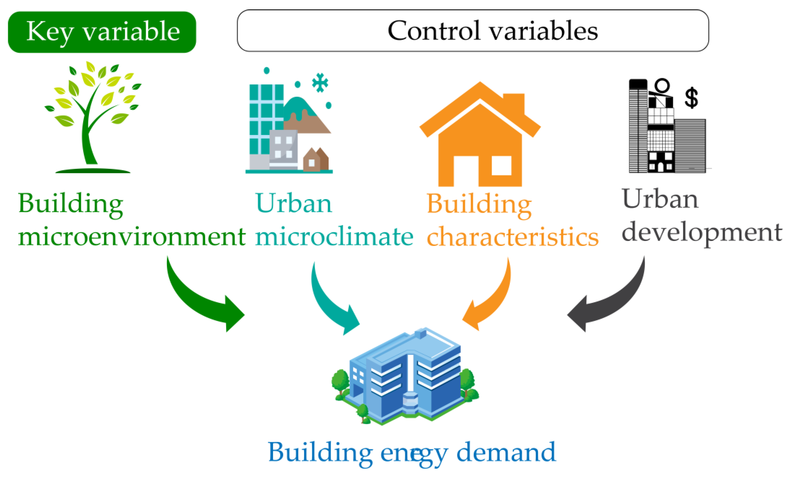
2. Theoretical Framework

2.1. Theoretical Framework of Energy Consumption in Government Office Buildings

The theoretical framework is a brief note about energy consumption in government office buildings, which is examined in this study (see Figure 1). Based on the analytical framework of the relationships between building energy consumption and urban system elements [9], we divided the factors that affect energy consumption in government office buildings into the following four categories: building microenvironment, building characteristics, urban microclimate, and urban development. The energy consumption in a government office building can be written as:
Q i = f ( BM , BC , UM , UD )
where Q i refers to the energy consumption in the government office building, I; BM is a vector of the building microenvironment; BC is a vector of the building characteristics; UM refers to measuring the urban temperature of the city where i is located; UD refers to the economic development of the city where i is located. Equation (1) provides the basis for empirical implementation of this study.
In this study, the key explanatory variable that we focused on was building microenvironment, and other variables were control variables (the detailed variables can be seen in Table 1). In terms of building microenvironment, we selected urban greenspace density, road density, and the number of POI (see Figure 2). Urban green spaces, roads, and buildings are clustered together in close spatial proximity. This adjacency and closeness of the variables can affect the energy consumption in urban buildings through mechanisms detailed in the following subsections.

2.2. Dependent Variables

In this study, we focused on the impacts of building microenvironment on building energy consumption (BEC). According to previous research, total building energy consumption is generally used to represent building energy demand [34]. Therefore, in this study, the dependent variable was the total annual government office building energy consumption.

2.3. Independent Variables

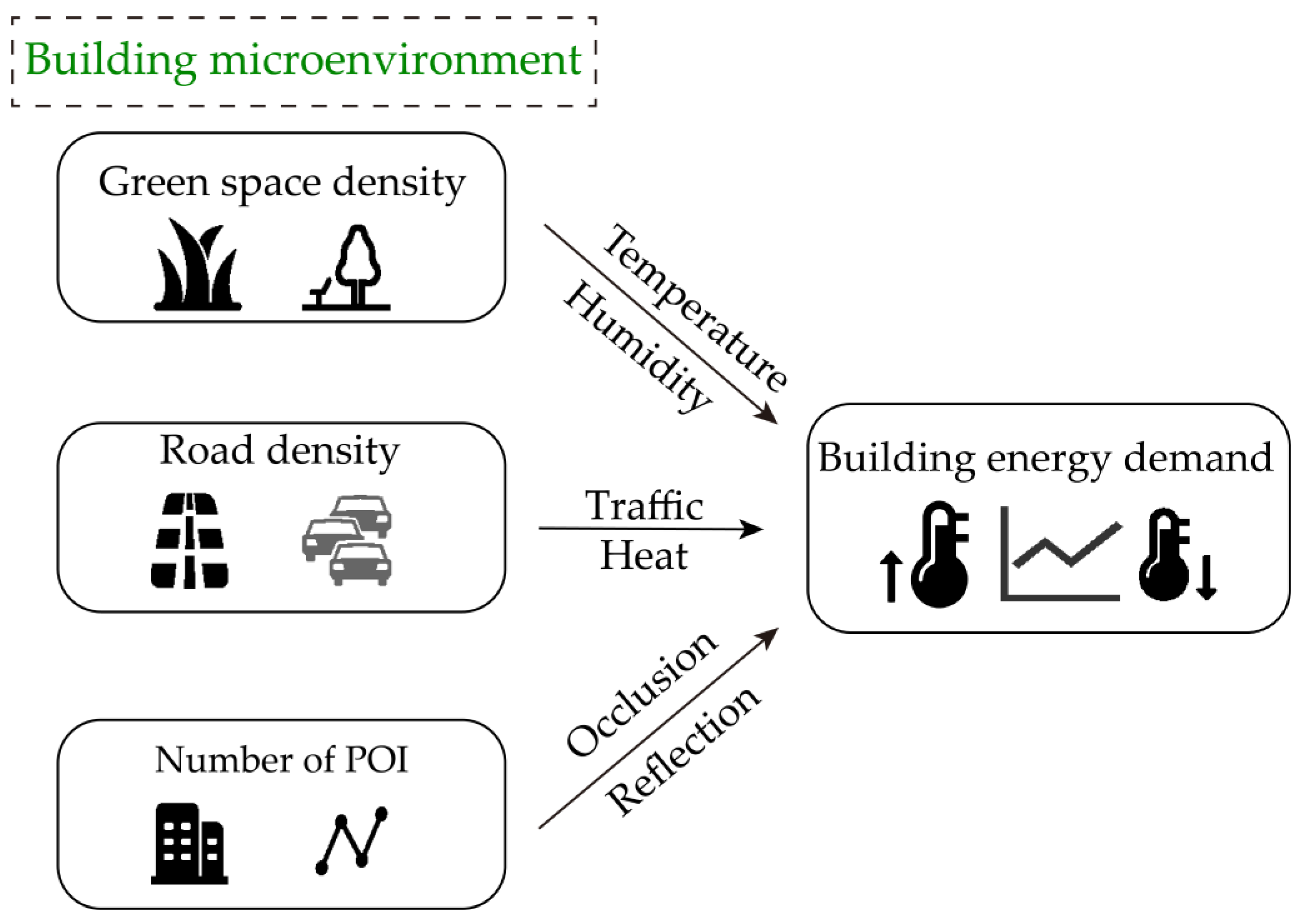
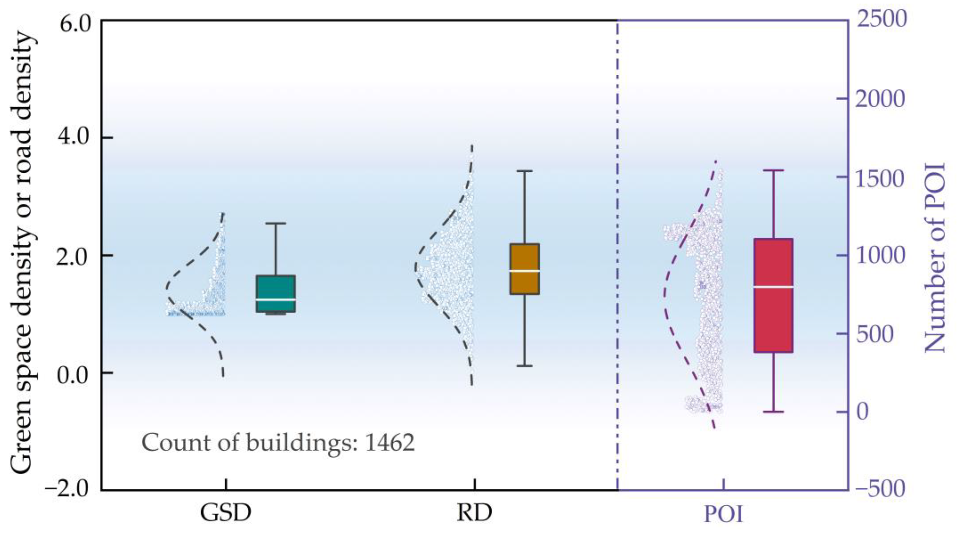
2.3.1. Building Microenvironment

Building microenvironment was the key explanatory variable in this study. Based on previous research [6,9], green space density, road density, and the number of POI around a building were selected to reflect the building’s microenvironment. The variables of greenspace density, road density, and the number of POI are introduced as follows:
We selected green space density (GSD) to reflect urban green space coverage. Previous research has shown that the existence of urban green spaces affects the surface temperature and humidity around a building [35,36], which, in turn, affects the building’s energy consumption. When measuring urban green space coverage, some scholars have previously calculated the proportions of fine-textured vegetation, coarse-textured vegetation, water bodies, impervious surfaces, and other urban greening types separately [12], while others have directly summarized these surface coverage into urban green spaces, and then calculated their area [37] or density [13,28]. These treatments yielded convincing results. Combined with previous research, we selected urban green space density.
Road density (RD) was selected to reflect the distribution of roads around a building. The distribution of roads around a building has been shown to be closely related to traffic heat, which is an important contributor to anthropogenic heat [38]. When the distribution of roads around a building is intricate, the probability of traffic heat being produced around the building increases. Ultimately, the microclimate around the building changes, thus, affecting the building’s energy consumption. When measuring the distribution of roads, Shivaram et al. (2021) adopted the number of adjacent roads and the mean distance of adjacent roads [9]. When considering the adjacency and distance of roads, we chose road density to characterize the distribution of roads. When the road density is higher, the distribution of roads is more likely to be intricate.
We selected the number of surrounding points of interest (POI) to reflect the proximity to other buildings. The proximity of other buildings can affect building energy consumption through occlusion or reflection [25,26]. It is typically conducted by simulating the height of buildings [39]. However, it is difficult to model thousands of buildings in multiple cities through simulations to reflect the height of other buildings around a building, and it is not possible to obtain information such as the surrounding building envelope structure. Therefore, we planned to select the number of POI around the government office buildings. The number of POI reflects the proximity and distribution of surrounding buildings. The greater the number of surrounding POI, the greater the probability of occlusion or reflection from other buildings impacting a government office building.

2.3.2. Urban Microclimate

Heating degree days and cooling degree days (CDDs) are important climatic factors that reflect changes in surface temperature. They are typically used to measure the microclimate of a city or province [40]. Our research region is Guangdong Province, which has a hot summer and warm winter. There is almost no heating demand. Therefore, only the CDDs were used to represent the urban microclimate.

2.3.3. Building Characteristics

Building characteristics such as building shape, building area (BA), and orientation can affect building energy consumption [34]. However, due to the limited availability of data, only the building area data were available.

2.3.4. Urban Development

Due to the location of government office buildings in different cities, to consider the differences between different cities, in this study, we introduced the proportion of urban tertiary industry (TE) to reflect the level of urban economic development. Therefore, we obtained the TE of each city to indicate the advanced level of the urban industrial structure and level of economic development.

3. Econometric Model and Data Description

3.1. Data Collection

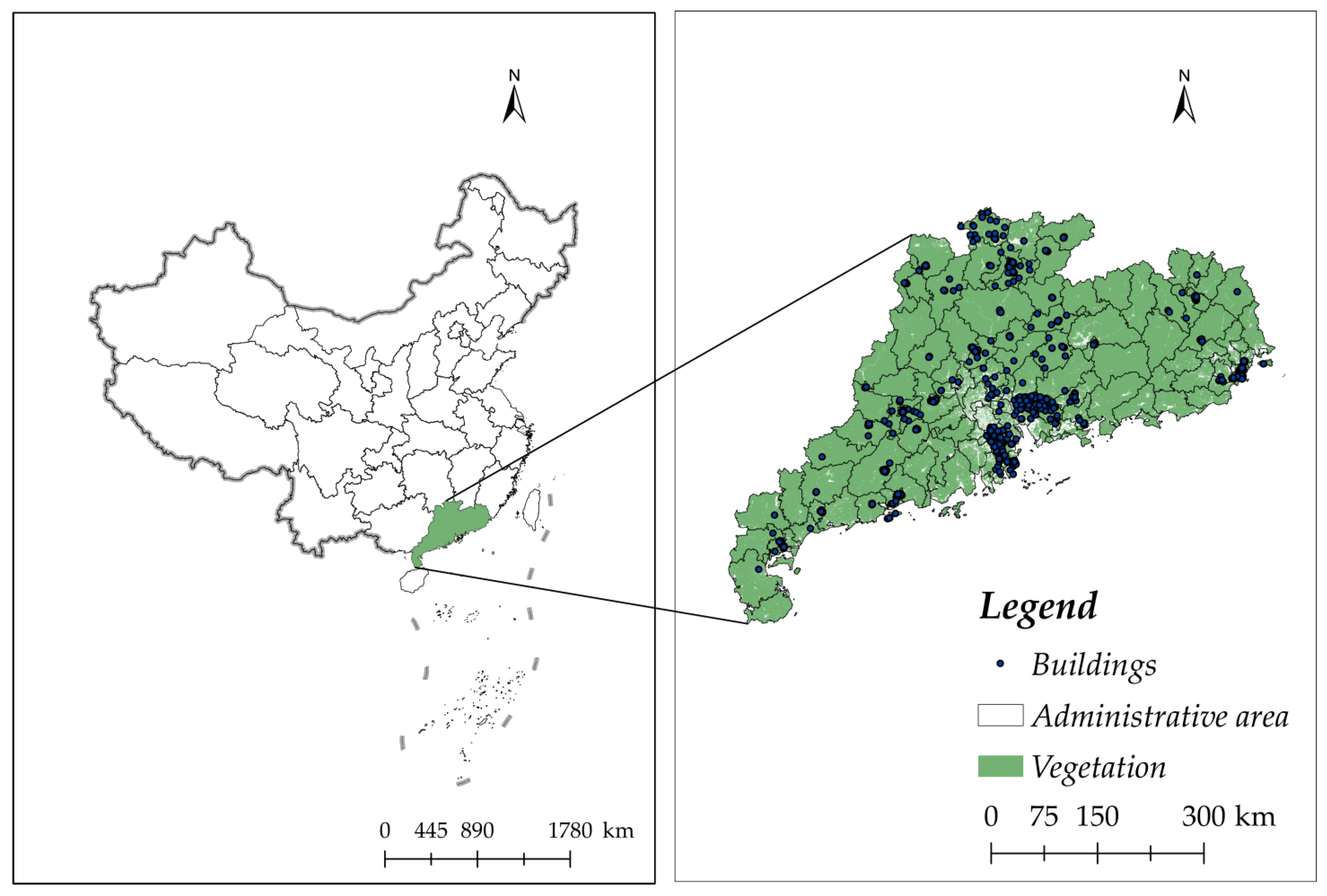
3.1.1. Research Area

The research area of this study was Guangdong Province. Guangdong Province is located in southern China, with an area of 179,700 square kilometers. As reported by the China Database of Building Energy Consumption and Carbon Emissions [41], building operation energy consumption in Guangdong Province was 95.3 million tce in 2020, accounting for about 10% of the total building operation energy consumption in China (as shown in Figure 3). The electricity consumption in Guangdong Province is 73.30 million tce, which accounts for 76.91% of building operation consumption in Guangdong Province. Among the public buildings, urban buildings, and rural buildings, the operation energy consumption of public buildings accounts for 43.9%. It can be seen that Guangdong is a large energy consumption province in China. The types of landforms in Guangdong Province are complex and diverse, including mountains, hills, terraces, and plains, which account for 33.7%, 24.9%, 14.2%, and 21.7% of the total land area of the province, respectively. Covering an area of approximately 16,630 square kilometers, the urban area in Guangdong Province has a comprehensive range of different elements, including residential areas, commercial areas, offices, parks, and rivers. Guangdong Province has established a public system for building energy consumption data to ensure the availability of research data. Therefore, Guangdong Province was chosen as the research area for this study.
In this study, a series of government office buildings were selected as the public buildings for this investigation. Public buildings include government office buildings, hotels, hospitals, and schools, and the energy consumption of the different types of buildings is closely related to the number of users. However, there is no public data available on the number of users of these buildings, and it is difficult to eliminate the impact of the number of users on energy consumption. Notably, government office buildings serve similar service management affairs, and the per capita floor area of government office buildings is similar with certain restrictions. Thus, the per capita building area of government office buildings can be considered to be the same. Therefore, selecting government office buildings as research objects can eliminate the influence of the number of users to a certain extent. Due to differences in the statistical caliber of different cities in Guangdong Province, few building characteristics have been publicly announced. For example, some cities have published the floors of public buildings, while others have not; some public building areas have been published, while other types of public buildings have been not published. Therefore, to obtain credible research results, we decided to only focus on government office buildings in Guangdong Province for which building areas had been published. In addition, to increase the sample size, we obtained data from 2015 to 2019. Public buildings publicized every year by cities in Guangdong Province during 2015 to 2019 were not consistent. For example, some building energy consumption data were publicized in 2015, but they were not continuously updated over the next few years, whereas some building energy consumption was only updated in a certain year. Therefore, in this study, we only retained the building energy consumption data for a certain year and treated the obtained data as cross-sectional data. Finally, 1462 government office buildings in 14 cities located in Guangdong Province from 2015 to 2019 were selected as the study samples (see Figure 4).
We focused on the operational energy consumption of government office buildings, which was mainly related to lighting, cooling, and other maintenance needs. The energy consumption of the government office buildings in this study refers to building electricity consumption. For the buildings, we collected the electricity consumption and building area. Building energy consumption and building characteristics were obtained from the websites of statistical bureaus or government websites of various cities in Guangdong Province. We geocoded the addresses of government office buildings through the API of Gaode Map to convert their addresses to coordinates. To build the microenvironment, we obtained information through multiple channels, such as the API of Gaode Map, GlobeLand30 dataset, national 1:250,000 basic geographic data, and geographic information system (GIS). For the control variables, we acquired information through the China Meteorological Science Professional Knowledge Service System and the city yearly statistical book.

3.1.2. Variables Processing

  • Building microenvironment
The building microenvironment variables included urban GSD, RD, and the number of POI. The existence and proximity of green spaces, roads, and buildings change the microclimate around buildings. The microclimate around a building usually refers to the local climate within 1000 m of the building [28], therefore, we selected urban green spaces, roads, and buildings within 1 km of a building.
For green space density, as performed in previous research, we selected the density of urban green spaces within 1 km of a building. The formula for calculating urban GSD is as follows:
GSD = A ( m 2 ) A total ( m 2 )
where A refers to the total area of urban green space within 1 km of a building and A total refers to an area of 1 km radius around a building. Urban green space includes six types of surface cover: cultivated land, forest, shrubland, wetland, and water bodies. This study used the GlobeLand30 dataset provided by the China Geographic Information Resource Directory Service System to calculate the urban green space area and the urban GSD within 1 km of a building using ArcGIS. The GlobeLand30 dataset with a resolution of 30 m is an important achievement of China’s National High-Tech Research and Development Program (863 Program) Global Land Cover Remote Sensing Mapping and Key Technology Research Project. The dataset contains ten main types of land cover: cultivated land, forest, shrubland, wetland, water body, tundra, artificial surface, bare land, glacier, and permanent snow. The urban green space referred to in this study included six types of surface cover: cultivated land, forest, shrubland, wetland, and water bodies. The urban green space coverage in Guangdong Province is shown in Figure 4. According to the box diagram shown in Figure 5, the median of GSD is 1.24, and most observations are below 1.24.
For road density, we refer to the length of a road per unit area. We calculated the total road length within 1 km of a building. The calculation formula for RD is as follows:
RD = L road ( km ) A total ( m 2 )
where L road refers to the total length of the road within 1 km of the building and Atotal refers to an area within 1 km radius of a building. In this study, road information was obtained through national 1:250,000 basic geographic data provided by the China Geographic Information Resource Directory Service System, and the road length and density within 1 km of the government office buildings were calculated using ArcGIS. According to the box diagram shown in Figure 5, the median of RD is 1.73, and the variables are generally a normal distribution.
For the number of POI, we calculated the number of POI within 1 km of the government office buildings. Through the API of Gaode Map (Goade Map is China’s leading provider of digital map content, navigation, and positioning services), the number of POI within 1 km of government office buildings were obtained. The types of POI selected in this study included residential communities, shopping malls, supermarkets, and banks. According to Figure 5, the median of POI is 798, and significant data are concentrated above 75% and below 25%.
2.
Other control variables
For the urban microclimate, we used the daily value dataset of China’s surface climate data provided by the China Meteorological Science Professional Knowledge Service System to calculate the cooling degree days in various cities of Guangdong Province. Regarding building characteristics, only building areas were available from the websites of statistical bureaus or government websites of various cities studied in Guangdong Province. For urban development, we obtained the proportion of the urban tertiary industry in different cities to eliminate the differences in the level of economic development between cities through the statistical yearbook of each city.

3.2. Econometric Model

Based on the theoretical framework of the mechanism of building microenvironment on the public building energy consumption described in Section 2, we investigated and empirically quantified the impacts of building microenvironment on building energy consumption using a multiple linear regression model. Following Shivaram et al. (2021) [9], the estimation model can be expressed as follows:
Y = α + i n β i X i + μ
where Y is the dependent variable. In this study, Y is building energy consumption; X I refers to the variables of the building microenvironment and control variables; α is the model intercept; I is the parameter that needs to be estimated, revealing the relationship between the independent and dependent variables; and μ is the interference term. To improve the heteroscedasticity of the model, the natural logarithm of the variable was introduced and the model was designed as follows:
ln ( Y ) = α + i n β i lnX i + + μ
Here, I i is expressed as the elasticity of the independent variable I to the dependent variable Y, that is, the percentage increase of the dependent variable caused by the percentage increase in X i . However, Formula (2) requires the value of the independent variable to be a value that is not 0. The time range of the data obtained in this study was from 2015 to 2019. Since the data were treated as cross-sectional data, in this study, we introduced the dummy variable of the publicity year to control for the time effect. To avoid multicollinearity, we used 2015 as a reference and converted 2016–2019 into dummy variables. Combined with the basic data information of each variable and the theoretical framework, the final ordinary least squared (OLS) model is designed as follows:
ln ( BEC ) = α + β 1 GSD + β 2 ln ( RD ) + β 3 ln ( POI ) + i n β i ln ( X i ) + i n δ i Y i + μ
where BEC refers to building energy consumption, GSD refers to urban GSD, POI refers to the number of POI, X i refers to the control variables, and Y i refers to the dummy variables of the year when building energy consumption data are publicized. As the minimum value of the urban GSD is 0, the natural logarithm cannot be taken; therefore, the variable of urban GSD has to take the original value. The key parameters that, in this study, we focused on were β 1 , β 2 , and β 3 . β 1 is the semi-elasticity coefficient, which refers to the percentage increase in building energy consumption for every unit increase in urban GSd. β 2 and β 3 refer to the percentage of increase in building energy consumption for every 1% increase in road density and the number of POI, respectively.

4. Results

The results demonstrate that the OLS model is robust. After estimating the parameters of Equation (5), some statistical indicators of the model were obtained, as shown in Table 2. R 2 is 0.723, which indicates that the selected variables of urban GSD, RD, the number of POI, CDDs, building area, and the proportion of the city’s tertiary industry can explain more than 70% of the energy consumption in government office buildings. The higher the R 2 , the higher the fit of the model. The adjusted R 2 is 0.721, which is similar to R 2 and is also an important key indicator for measuring model quality. The variance analysis showed that the F value of the model was 467.6 and the corresponding p-value was 0.000, with a significance level that was below 5%. The fitted multiple linear regression equation is statistically significant, indicating the validity of the model. After estimating the model, a white test was adopted to test the hypothesis of homoscedasticity. As shown in Table 2, the results of the white test show that the white test statistic is 188.56, and its significance level is below 5%, which rejects the hypothesis of model homoscedasticity. Therefore, it is considered that the model is heteroscedastic. Therefore, we adopted a robust standard error to estimate Equation (5).
The parameter estimation results obtained using robust standard errors are shown in Table 3. Most of the variables were found to be significant at the 5% level.
In this study, the core explanatory variables that we focused on were the building microenvironment elements, which were specifically expressed as GSD, RD, and the number of POI around the building. Greenspace density has a significant negative impact on the energy consumption in government office buildings. It can be seen from Table 3 that the p-value of GSD is 0.002, which is less than 5%, indicating that GSD is statistically significant at the 5% significance level. The coefficient of GSD is −0.227, which means that when other variables are controlled, building energy consumption is reduced by 0.277% with an increase in GSD by one unit. The higher the greenspace density, the lower the building energy consumption, which is consistent with previous research [23,42].
Unlike GSD, RD has a significant positive impact on government office building energy consumption. The variable coefficient of RD is 0.298 and its significance is 0.000, which is statistically significant at the 5% significance level. For every 1% increase in RD, building energy consumption increases by 0.288%. The increase in RD around buildings leads to an increase in building energy consumption.
The variable of POI has a significant positive impact on building energy consumption. In other words, building energy consumption increases with an increase in the number of POI. The coefficient of the POI is 0.05 (the p-value is 0.012, which is statistically significant at the 5% level of significance), indicating that an increase of 1% in the number of POI within 1 km of the building increases the building energy consumption by 0.048%. The number of POI is a key variable reflecting building density, which means that building density is positively correlated with building energy consumption, which is consistent with the findings from the study of Z. Ye, Cheng, Hsu, Wei, and Cheung (2021) [43]. The denser the building, the higher the building energy consumption.
For the other control variables, the impacts on building energy consumption were positive. CDDs have a significantly positive impact on building energy consumption. The building energy consumption increases by 1.258% when the cooling degree days increase by 1%. This is because Guangdong Province has hot summers and warm winters, with a large cooling demand and high energy consumption for air conditioning and refrigeration. Therefore, the higher the CDDs, the higher the building energy consumption. For every 1% increase in building area, building energy consumption also increases by 1.02%. In addition, building energy consumption increases as the proportion of the city’s tertiary industry increases. In other words, building energy consumption is closely related to the economic development level of a city.

5. Discussion

5.1. Relationships between Building Microenvironment and Energy Consumption in Government Office Buildings

In contrast to previous simulation-based methods (as shown in Table 4), we adopted a regression analysis method to study the relationships between building microenvironment and building energy consumption. First, we extracted a building’s microenvironment elements present from the actual location, and then used the government office buildings as the object to study the impacts of urban GSD, RD, and the number of POI on building energy consumption, which made the research more efficient. Urban GSD, RD, and the number of POI characterize the building’s microenvironment. The adjacency and closeness of these elements are closely related to the microclimate around the building, which, in turn, affects the energy consumption in the building.
With the expansion of cities and economic development, the local climate of cities has changed and environmental conditions have continued to deteriorate. The heat island effect and air pollution problems have had a negative impact on the quality of life of residents and on the sustainable development of cities. The emergence of urban green spaces has mitigated these adverse effects and further affected building energy consumption. The results of this study indicate that the density of urban green spaces significantly increases building energy consumption. Urban green space coverage mainly comprises urban parks, urban greenery, and water bodies. On the one hand, the existence of urban green spaces increases air humidity and effectively reduces surface temperature, thereby, reducing the indoor cooling demand and energy consumption in a building. Evyatar and Bin (2022) showed that the implementation of an extensive planting strategy would reduce the annual average temperature by approximately 0.3 °C and save energy by about 2–3% [44]. Similar findings have also been confirmed by Zardo et al. (2017) [45]. As compared with areas lacking urban green space, higher green space coverage is conducive to maintaining the stability of the surrounding microclimate and reducing energy consumption. On the other hand, the presence of trees provides shade from the sun to a certain extent, and also reduces the temperature of the block [46], thereby, reducing building energy consumption. Dense green space coverage is beneficial for reducing the impact of the urban heat island effect, reducing cooling requirements, and thereby, reducing building energy consumption.
Urban green spaces reduce building energy consumption, whereas a dense distribution of roads increases building energy consumption. A dense distribution of roads is closely linked to higher building energy consumption. Road density refers to the traffic flow around a building. A higher RD around a building is correlated with higher car mobility. Carbon dioxide and other greenhouse gases produced by various cars on the road cause the surrounding temperature to increase [48]. As the ambient temperature increases, the traffic heat effect increases, which ultimately leads to an increase in building energy consumption. However, this is contrary to the findings of Shivaram et al. (2021) who found that the more roads there were near a building, the lower the building energy consumption [9]. This appears to be contrary to the increase in building energy consumption caused by traffic heat. These results may be based on a specific urban context. Therefore, it is necessary to encourage research on the relationship between RD and building energy consumption in more cities.
Similar to the density of road distribution, building microenvironment formed by the proximity of surrounding buildings increases building energy consumption. The higher the number of POI around a building, the higher the energy consumption in the building. The number of POI reflects the proximity to the building to a certain extent. The greater the number of POI, the stronger the inter-building effect of mutual occlusion between buildings and the reflection of the building shell. Thus, the energy consumption for lighting and cooling increases. This finding can be supported by the study of Liu et al. (2015), which found that as the density of urban planning increased, the shading effect significantly affected energy consumption, and heating energy consumption increased by 32% [47]. In addition, with the development of a city, its social and economic activities do not appear to have a single-center distribution. There are multiple subcenters in a city. The number of POI around the buildings selected in this study also reflects the intensity of the social and economic activities at the locations of the buildings. The greater the number of POI, the higher the socioeconomic intensity, and the stronger the heat island effect of the location of a building [49]. Therefore, more building energy is used for cooling.

5.2. Heterogeneous Impacts of Building Microenvironment on Energy Consumption in Government Office Buildings via the Scale of the Building

The research results show that the larger the building area, the higher the total energy consumption in the government office building. Notably, the energy supply of public buildings is closely related to the building scale. For example, large-scale public buildings usually adopt centralized energy supply methods such as central air conditioning. Centralized energy supply methods always maintain constant energy consumption, and the energy consumption in larger-scale buildings may not be as sensitive to changes in the external environment as buildings of smaller scale. Therefore, any heterogeneity in the energy consumption change of different-scale government office buildings caused by the change in the building microenvironment around the building needs to be invested.
To explore the heterogeneous impacts of building microenvironment on building energy consumption in government office buildings of different scales, we adopted building area as the threshold variable for the threshold regression. The coefficient of the threshold regression indicates the degree of impact of the independent variable on the dependent variable when it is greater than or less than the threshold value. According to the research of Hansen (2000) [50], we used the bootstrap method to calculate the Lagrange multiplier (LM) statistics and p-value; the bootstrap frequency was set to 500, and the sample reduction ratio was set to 15% when testing the threshold. The threshold test and regression show that the data have a threshold effect (as shown in Figure 6 and Table 5), and the threshold value is 2323. Table 6 presents the results of the threshold regression.
As shown in Table 6, there are evident differences in the impacts of building microenvironment on building energy consumption in government office buildings of different scales. Regarding GSD, as the building area increases, the absolute value of the GSD variable coefficient decreases. At the same time, its significance decreases, showing that the impact of greenspace density on building energy consumption decreases with an increase in building scale. In other words, GSD has less impact on government office building energy consumption on a larger scale than on government office energy consumption on a smaller scale. This may be because the public areas of large-scale government office buildings account for a large proportion of the energy consumption, which does not change with the external environment. For government office buildings, part of the building energy consumption is closely related to public areas, such as corridor lighting, lighting, air conditioning, and refrigeration in public areas rather than personal office areas. However, this portion of the energy consumption is closely related to the building scale. When the building scale is large, the public area is large, resulting in a large proportion of stable energy consumption in the public areas. Although an increase in greenspace density promotes a reduction in building energy consumption, the energy consumption in public areas does not change with the external environment. Therefore, an increase in GSD results in smaller changes in the energy consumption of large-scale government office buildings as compared with small-scale buildings.
Similar to GSD, RD has less impact on the energy consumption of larger-scale government office buildings. Although the significance level of the variable of road density in different sample groups is less than 5%, when the building area shifts from being less than the first threshold to being greater than the first threshold, the coefficient of RD gradually decreases, which shows that the impact of RD on energy consumption in government office buildings decreases with an increase in building scale. This is similar to the mechanism of green space coverage on the energy consumption in large-scale government buildings. Building energy consumption is closely related to area (such as cooling energy consumption in public areas) and increases with an increase in building scale, but this part of the energy consumption does not change with changes in the external environment. As road density increases, the amount of traffic heat that causes the outside temperature to rise continues to increase; this part of the energy consumption is not changed significantly. As compared with small-scale government office buildings, the public areas of large-scale buildings consume more energy. This part of the energy is barely affected by external changes, resulting in a smaller change in energy consumption. Therefore, RD had less impact on the energy consumption in large-scale government office buildings. However, owing to the direction in which the heat flow moves, the temperature distribution gradually decreases. With an increase in RD, the heat effect of traffic causes the outdoor temperature to increase. When the building envelope transfers heat from a place with a high outdoor temperature to a place with a low indoor temperature, the temperature decreases gradually. In the case of a large-scale building, the heat may not pass to the central part of the building; therefore, the central area inside the building is not affected. That is, in a large-scale government office building, less space is affected by an increase in outdoor temperature as compared with the whole building, and therfore, the energy consumption change is smaller.
It can also be seen from Table 6 that the impact of the number of POI on building energy consumption in government office buildings of different scales is also clearly heterogeneous. The number of POI has no significant impact on small-scale buildings, but it has a significant impact on large-scale buildings. When the building area is less than the first threshold, the impact of the number of POI on building energy consumption is not significant. However, when the building area is larger than the first threshold, the impact of the number of POI on building energy consumption becomes significant (the significance level is at 5% or less). The number of POI has a positive impact on building energy consumption, which is similar to the OLS results. This implies that the number of POI has a greater impact on the energy consumption in large-scale government office buildings. According to the previous discussion, changes in the external environment have less impact on the energy consumption of large-scale buildings. Similarly, the number of POI should have a greater impact on smaller building areas, but the results of this study show that the impact is not significant. This may be because the government office buildings with a relatively small scale may be located in economically underdeveloped cities or at the outskirts of cities, where the number of POI is relatively small and the building proximity represented by the number of POI is not evident. Therefore, the number of POI does not have a significant impact on the energy consumption in small-scale government office buildings. However, more work needs to be done to quantify and analyze the impact of building proximity on building energy consumption in suburban or downtown areas.

6. Conclusions

The adjacency and closeness of urban green spaces, the density of the distribution of roads, and proximity to other buildings form a building’s microenvironment, thus, affecting the building’s energy consumption. Based on energy consumption data of government office buildings in Guangdong Province, in this study, we used a regression analysis method to explore the impact mechanism of building microenvironment on building energy consumption at the level of individual buildings in different cities. Our research results confirm some of the findings of previous simulation-based research and also provide novel findings. For example, when other variables remain unchanged, the higher the density of urban green space coverage around the buildings, the lower the energy consumption in government office buildings, which is similar to previous research [29]. Higher road density is correlated with higher energy consumption in government office buildings. Government office buildings with more POI also consume more energy. These elements affect the energy consumption inside a building by changing the outdoor microclimate. In addition, in this study, we also found that urban GSD and RD had less impact on government office buildings on a larger scale. This may be due to the larger fixed energy consumption in government office buildings. This part of the fixed energy consumption is closely related to building scale and is not easily affected by the external environment. However, contrary to GSD and RD, the number of POI had no significant impact on the energy consumption in small-scale government office buildings, whereas it had a significant impact on the energy consumption in large-scale government office buildings. This may be because, in economically underdeveloped cities or urban suburbs, the number of POI is relatively small, which is insufficient to reflect the impact of building proximity. Therefore, more work is needed to quantify and analyze the impact of building distance on building energy consumption in suburban or downtown areas.
Overall, the empirical data-driven analysis method used in this study improves the efficiency of carrying out the research, and the research findings can provide support for realizing the scientific planning and layout of urban green landscapes and infrastructure, as well as formulating energy conservation and emission reduction policies. For example, based on the impacts of building microenvironment on building energy consumption and when optimizing urban structure and layout, the overall layout of ecological corridors, landscape viewing corridors, waterfront spaces, and urban greenways should be strengthened. The layout of urban expressways and transportation of living spaces should be arranged rationally. This is based on the heterogeneous impacts of building microenvironment on energy consumption in buildings of different scales. The scale of new public buildings should also be controlled to improve energy efficiency. These research findings indicate how urban green landscapes and the use of urban land can be rationally planned to build a green and low-carbon city.
In contrast to previous studies, in this study, we proposed an empirical method to evaluate the impacts of building microenvironment on building energy consumption. GSD, RD, and the number of POI were selected to reflect changes in the building microenvironment. However, our study has some limitations. First, although the energy consumption data were from government departments, the published data were not panel data and lacked building characteristics such as orientation, floor height, and building materials. Therefore, the impacts of unobservable variables on building energy consumption cannot be eliminated, and an energy consumption database that includes additional building characteristics should be established. Second, a building’s microenvironment includes not only urban green space coverage, RD, and the number of POI, but also microscopic factors such as wind and thermal environments. However, owing to the availability of data and the limitations of research scales, it is not possible to evaluate the impacts of meteorological factors such as wind speed and thermal radiation on building energy consumption. Therefore, it is necessary to comprehensively consider various urban factors contributing to changes in the surrounding building microenvironment in future research to overcome this issue. Finally, it is essential that the application of this analysis to urban planning and decision support is explored in depth. Future work should aim to transform the analysis results into actionable opinions on sustainable urban design, management, and operation, such as establishing a monitoring platform for urban energy consumption data, using sensor technology to identify changes in the building microenvironment, and adopting machine learning techniques to describe the relationships between building microenvironment and building energy consumption.

Author Contributions

Z.L., Methodology, formal analysis, writing—original draft; S.P., Validation, Writing—review and editing, Visualization; W.C., Conceptualization, supervision, funding acquisition; S.C., Formal analysis, investigation, validation; X.W., Writing—review and editing; R.L., Software, visualization; X.M., data curation, funding acquisition. All authors have read and agreed to the published version of the manuscript.

Funding

This research was funded by the National Key R&D Program of China, grant number 2018YFD1100203 and the Social Science Planning Project of Chongqing, grant number 2019QNGL30.

Data Availability Statement

Not applicable.

Acknowledgments

We thank the editor and anonymous referees, whose remarks have been very constructive and inspiring in preparing the final version of the paper. We are solely responsible for the opinions expressed in this paper.

Conflicts of Interest

The authors declare no conflict of interest.

References

  1. Li, R.; Yu, Y.; Cai, W.; Liu, Q.; Liu, Y.; Zhou, H. Interprovincial differences in the historical peak situation of building carbon emissions in China: Causes and enlightenments. J. Environ. Manag. 2023, 332, 117347. [Google Scholar] [CrossRef] [PubMed]
  2. CABEE. China Building Energy Consumption Annual Report 2021; China Association of Buiding Energy Efficency: Beijing, China, 2021. [Google Scholar]
  3. Jiang, Y.; Yan, D.; Guo, S.; Hu, S. China Building Energy Use 2018; China Architecture Publishing & Media Co., Ltd.: Beijing, China, 2018; p. 42. [Google Scholar]
  4. Jiang, Y.; Zhang, Y.; Guo, S.; Xia, J.; Wei, Q.; Zheng, W.; Zhang, Y.; Yin, S.; Fang, H.; Deng, J. 2020 Annual Report on China Building Energy Efficiency; China Architecture & Building Press: Beijing, China, 2020. [Google Scholar]
  5. Amir, K.; Ram, R.; Martin, F. Determinants of residential electricity consumption: Using smart meter data to examine the effect of climate, building characteristics, appliance stock, and occupants’ behavior. Energy 2013, 55, 184–194. [Google Scholar] [CrossRef]
  6. Hiroshi, Y.; Tianzhen, H.; Natasa, N. IEA EBC annex 53: Total energy use in buildings—Analysis and evaluation methods. Energy Build. 2017, 152, 124–136. [Google Scholar] [CrossRef]
  7. Zheng, Y.; Ali, G.; Burcin, B.-G. Building occupancy diversity and HVAC (heating, ventilation, and air conditioning) system energy efficiency. Energy 2016, 109, 641–649. [Google Scholar] [CrossRef]
  8. Zhou, Y.; Gurney, K. A new methodology for quantifying on-site residential and commercial fossil fuel CO2 emissions at the building spatial scale and hourly time scale. Carbon Manag. 2010, 1, 45–56. [Google Scholar] [CrossRef]
  9. Shivaram, R.; Yang, Z.; Jain, R.K. Context-aware Urban Energy Analytics (CUE-A): A framework to model relationships between building energy use and spatial proximity of urban systems. Sustain. Cities Soc. 2021, 72, 102978. [Google Scholar] [CrossRef]
  10. Changzhi, D.; Li, L.; Zhiwei, L. Method for the determination of optimal work environment in office buildings considering energy consumption and human performance. Energy Build. 2014, 76, 278–283. [Google Scholar] [CrossRef]
  11. Grossmann, D.; Galvin, R.; Weiss, J.; Madlener, R.; Hirschl, B. A methodology for estimating rebound effects in non-residential public service buildings: Case study of four buildings in Germany. Energy Build. 2016, 111, 455–467. [Google Scholar] [CrossRef]
  12. Du, S.; Xiong, Z.; Wang, Y.-C.; Guo, L. Quantifying the multilevel effects of landscape composition and configuration on land surface temperature. Remote Sens. Environ. 2016, 178, 84–92. [Google Scholar] [CrossRef]
  13. Park, J.; Kim, J.-H.; Lee, D.K.; Park, C.Y.; Jeong, S.G. The influence of small green space type and structure at the street level on urban heat island mitigation. Urban For. Urban Green. 2017, 21, 203–212. [Google Scholar] [CrossRef]
  14. Sijie, Z.; Yue, Y.; Yu, Y.; Francesco, C.; Xing, J.; Xin, Z.; Xing, S. An evidence-based framework for designing urban green infrastructure morphology to reduce urban building energy use in a hot-humid climate. Build. Environ. 2022, 219, 109181. [Google Scholar] [CrossRef]
  15. Belčáková, I.; Świąder, M.; Bartyna-Zielińska, M. The Green infrastructure in cities as a tool for climate change adaptation and mitigation: Slovakian and Polish experiences. Atmosphere 2019, 10, 552. [Google Scholar] [CrossRef]
  16. Pamukcu-Albers, P.; Ugolini, F.; La Rosa, D.; Grădinaru, S.R.; Azevedo, J.C.; Wu, J. Building green infrastructure to enhance urban resilience to climate change and pandemics. Landsc. Ecol. 2021, 36, 665–673. [Google Scholar] [CrossRef]
  17. Qiao, R.L.; Liu, T.T. Impact of building greening on building energy consumption: A quantitative computational approach. J. Clean. Prod. 2020, 246, 119020. [Google Scholar] [CrossRef]
  18. Katia, P.; Adriano, M. Effects of vegetation, urban density, building height, and atmospheric conditions on local temperatures and thermal comfort. Urban For. Urban Green. 2014, 13, 495–506. [Google Scholar] [CrossRef]
  19. Amir, A. Assessment of green roof benefits on buildings’ energy-saving by cooling outdoor spaces in different urban densities in arid cities. Energy 2021, 219, 119514. [Google Scholar] [CrossRef]
  20. Mingfang, T.; Xing, Z. Experimental study of the thermal performance of an extensive green roof on sunny summer days. Appl. Energy 2019, 242, 1010–1021. [Google Scholar] [CrossRef]
  21. Ye, H.; Qiu, Q.; Zhang, G.; Lin, T.; Li, X. Effects of natural environment on urban household energy usage carbon emissions. Energy Build. 2013, 65, 113–118. [Google Scholar] [CrossRef]
  22. Ye, H.; Hu, X.; Ren, Q.; Lin, T.; Li, X.; Zhang, G.; Shi, L. Effect of urban micro-climatic regulation ability on public building energy usage carbon emission. Energy Build. 2017, 154, 553–559. [Google Scholar] [CrossRef]
  23. Aboelata, A.; Sodoudi, S. Evaluating urban vegetation scenarios to mitigate urban heat island and reduce buildings’ energy in dense built-up areas in Cairo. Build. Environ. 2019, 166, 106407. [Google Scholar] [CrossRef]
  24. Zhu, R.; Wong, M.S.; Guilbert, É.; Chan, P.-W. Understanding heat patterns produced by vehicular flows in urban areas. Sci. Rep. 2017, 7, 16309. [Google Scholar] [CrossRef]
  25. Pigliautile, I.; Chàfer, M.; Pisello, A.L.; Pérez, G.; Cabeza, L.F. Inter-building assessment of urban heat island mitigation strategies: Field tests and numerical modelling in a simplified-geometry experimental set-up. Renew. Energy 2020, 147, 1663–1675. [Google Scholar] [CrossRef]
  26. Vallati, A.; Mauri, L.; Colucci, C. Impact of shortwave multiple reflections in an urban street canyon on building thermal energy demands. Energy Build. 2018, 174, 77–84. [Google Scholar] [CrossRef]
  27. Mehaoued, K.; Lartigue, B. Society. Influence of a reflective glass façade on surrounding microclimate and building cooling load: Case of an office building in Algiers. Sustain. Cities Soc. 2019, 46, 101443. [Google Scholar] [CrossRef]
  28. Han, Y.; Taylor, J.E.; Pisello, A.L. Exploring mutual shading and mutual reflection inter-building effects on building energy performance. Appl. Energy 2017, 185, 1556–1564. [Google Scholar] [CrossRef]
  29. Gülten, A.; Aksoy, U.T.; Öztop, H.F. Influence of trees on heat island potential in an urban canyon. Sustain. Cities Soc. 2016, 26, 407–418. [Google Scholar] [CrossRef]
  30. Xuemiao, W.; Qingyan, M.; Linlin, Z.; Die, H. Evaluation of urban green space in terms of thermal environmental benefits using geographical detector analysis. Int. J. Appl. Earth Obs. Geoinf. 2021, 105, 102610. [Google Scholar] [CrossRef]
  31. Chen, Y.; Hong, T.; Piette, M.A. Automatic generation and simulation of urban building energy models based on city datasets for city-scale building retrofit analysis. Appl. Energy 2017, 205, 323–335. [Google Scholar] [CrossRef]
  32. Pisello, A.L.; Castaldo, V.L.; Poli, T.; Cotana, F. Simulating the thermal-energy performance of buildings at the urban scale: Evaluation of inter-building effects in different urban configurations. J. Urban Technol. 2014, 21, 3–20. [Google Scholar] [CrossRef]
  33. Gilani, S.; O’Brien, W.; Gunay, H.B. Simulating occupants’ impact on building energy performance at different spatial scales. Build. Environ. 2018, 132, 327–337. [Google Scholar] [CrossRef]
  34. Wang, X.; Fang, Y.; Cai, W.; Ding, C.; Xie, Y. Heating demand with heterogeneity in residential households in the hot summer and cold winter climate zone in China—A quantile regression approach. Energy 2022, 247, 123462. [Google Scholar] [CrossRef]
  35. Privitera, R.; Evola, G.; La Rosa, D.; Costanzo, V. Green infrastructure to reduce the energy demand of cities. In Urban Microclimate Modelling for Comfort and Energy Studies; Springer: Cham, Switzerland, 2021; pp. 485–503. [Google Scholar]
  36. Saaroni, H.; Amorim, J.H.; Hiemstra, J.; Pearlmutter, D. Urban Green Infrastructure as a tool for urban heat mitigation: Survey of research methodologies and findings across different climatic regions. Urban Clim. 2018, 24, 94–110. [Google Scholar] [CrossRef]
  37. Vaz Monteiro, M.; Doick, K.J.; Handley, P.; Peace, A. The impact of greenspace size on the extent of local nocturnal air temperature cooling in London. Urban For. Urban Green. 2016, 16, 160–169. [Google Scholar] [CrossRef]
  38. Afshin, A.; Fernanda, S.; Prashanth, M. Estimation of the traffic related anthropogenic heat release using BTEX measurements —A case study in Abu Dhabi. Urban Clim. 2018, 24, 311–325. [Google Scholar] [CrossRef]
  39. Anna Laura, P.; John, E.T.; Xiaoqi, X.; Franco, C. Inter-building effect: Simulating the impact of a network of buildings on the accuracy of building energy performance predictions. Build. Environ. 2012, 58, 37–45. [Google Scholar] [CrossRef]
  40. Huo, T.; Cao, R.; Du, H.; Zhang, J.; Cai, W.; Liu, B. Nonlinear influence of urbanization on China’s urban residential building carbon emissions: New evidence from panel threshold model. Sci. Total Env. 2021, 772, 145058. [Google Scholar] [CrossRef] [PubMed]
  41. CABEE. China Building Energy Consumption Annual Report 2022; China Association of Buiding Energy Efficency: Beijing, China, 2022. [Google Scholar]
  42. Aboelata, A. Vegetation in different street orientations of aspect ratio (H/W 1:1) to mitigate UHI and reduce buildings’ energy in arid climate. Build. Environ. 2020, 172, 106712. [Google Scholar] [CrossRef]
  43. Ye, Z.; Cheng, K.; Hsu, S.-C.; Wei, H.-H.; Cheung, C.M. Identifying critical building-oriented features in city-block-level building energy consumption: A data-driven machine learning approach. Appl. Energy 2021, 301, 117453. [Google Scholar] [CrossRef]
  44. Evyatar, E.; Bin, Z. The effect of increasing surface cover vegetation on urban microclimate and energy demand for building heating and cooling. Build. Environ. 2022, 213, 108867. [Google Scholar] [CrossRef]
  45. Zardo, L.; Geneletti, D.; Pérez-Soba, M.; Van Eupen, M. Estimating the cooling capacity of green infrastructures to support urban planning. Ecosyst. Serv. 2017, 26, 225–235. [Google Scholar] [CrossRef]
  46. Morakinyo, T.E.; Dahanayake, K.W.D.K.C.; Adegun, O.B.; Balogun, A.A. Modelling the effect of tree-shading on summer indoor and outdoor thermal condition of two similar buildings in a Nigerian university. Energy Build. 2016, 130, 721–732. [Google Scholar] [CrossRef]
  47. Liu, J.; Heidarinejad, M.; Gracik, S.; Srebric, J. The impact of exterior surface convective heat transfer coefficients on the building energy consumption in urban neighborhoods with different plan area densities. Energy Build. 2015, 86, 449–463. [Google Scholar] [CrossRef]
  48. Nocera, S.; Ruiz-Alarcón-Quintero, C.; Cavallaro, F. Assessing carbon emissions from road transport through traffic flow estimators. Transp. Res. Part C Emerg. Technol. 2018, 95, 125–148. [Google Scholar] [CrossRef]
  49. Min, M.; Lin, C.; Duan, X.; Jin, Z.; Zhang, L. Spatial distribution and driving force analysis of urban heat island effect based on raster data: A case study of the Nanjing metropolitan area, China. Sustain. Cities Soc. 2019, 50, 101637. [Google Scholar] [CrossRef]
  50. Hansen, B.E. Sample splitting and threshold estimation. Econometrica 2000, 68, 575–603. [Google Scholar] [CrossRef] [Green Version]
Figure 1. Factors that affect energy consumption in government office buildings.
Buildings 13 00481 g001
Figure 2. Theoretical framework of the impacts of building microenvironment on building energy consumption.
Buildings 13 00481 g002
Figure 3. Building operation energy consumption of Guangdong Province.
Buildings 13 00481 g003
Figure 4. Vegetation coverage and sample distribution in Guangdong Province.
Buildings 13 00481 g004
Figure 5. Box diagram of variables of building microenvironment.
Buildings 13 00481 g005
Figure 6. Likelihood ratio diagram with the threshold variable of BA.
Buildings 13 00481 g006
Table 1. Summary of variables.
ClassificationVariablesUnitImplications
Dependent variableBECKw·hBuilding electricity consumption
Building microenvironmentGSD Urban green space density within 1 km around the building, including cultivated land, forest, shrubland, wetland, water body
RDkm/m2Road density within 1 km around the building
POI The number of POI within 1 km of the building, including residential quarters, shopping malls, supermarkets, banks
Urban microclimateCDDsDay·CelsiusCooling degree days
Building characteristicsBAm2Building area
Urban developmentTE Industrial structure, proportion of urban tertiary industry
Table 2. Model summary.
R 2 Adjusted   R 2 FHeteroskedasticity Test (White)
0.7230.721467.6 ***188.56 ***
*** Indicates significant at the 1% level.
Table 3. Results of regression modeling.
LN(BEC)βRobust
Standard Error
Tp
GSD−0.227 0.074 −3.050 0.002
LN(RD)0.298 0.062 4.800 0.000
LN(POI)0.048 0.020 2.410 0.016
LN(CDD)1.258 0.140 9.010 0.000
LN(BA)0.995 0.017 58.760 0.000
LN(TE)1.577 0.203 7.770 0.000
YEAR1−0.074 0.059 −1.270 0.205
YEAR2−0.203 0.057 −3.540 0.000
YEAR3−0.155 0.069 −2.250 0.024
YEAR4−0.205 0.088 −2.310 0.021
CONSTANT−2.5800.823−3.1400.002
Note: Taking 2015 as a reference, YEAR1 refers to whether the publicity year is 2016. If yes, it is 1; otherwise, it is 0. YEAR2 refers to whether the publicity year was 2017, YEAR3 refers to whether the publicity year was 2018, and YEAR4 refers to whether the publicity year was 2019.
Table 4. Summary of methods used and conclusions found in previous studies.
CategoryMethodConclusion
Urban green spaceComputer simulationImplementing a strategy of extensive planting, so that a green surface fraction of 0.5 is obtained, results in a mean annual temperature reduction of about 0.3 °C and an energy saving relative to the current condition of about 2–3% [44].
Review of literature, case studyTree canopy coverage is one of the components that mainly determine the cooling capacity of a green urban infrastructures [45].
Computer simulationTree shade around buildings improves indoor and outdoor thermal conditions and comfort, and reduces energy expenditure [46].
Road distributionMultivariate multiple regressionAn additional proximate road is associated with a decrease in mean building energy consumption by 3.732 percent and with a decrease in the standard deviation of energy consumption by 7.560 percent, controlling for all other variables [9].
The proximity of other buildingsComputer simulationAir temperature surrounding a building significantly increases due to the multiple reflections of the radiation heat flux, leading to an increase in the cooling demand [27].
Computer simulationImpact of shading inter-building effect (IBE) on building energy usage is greater than reflection IBE [28].
Computer simulationWhen the plan area density increased, the total cooling energy consumption increased, and the total heating energy consumption decreased [47].
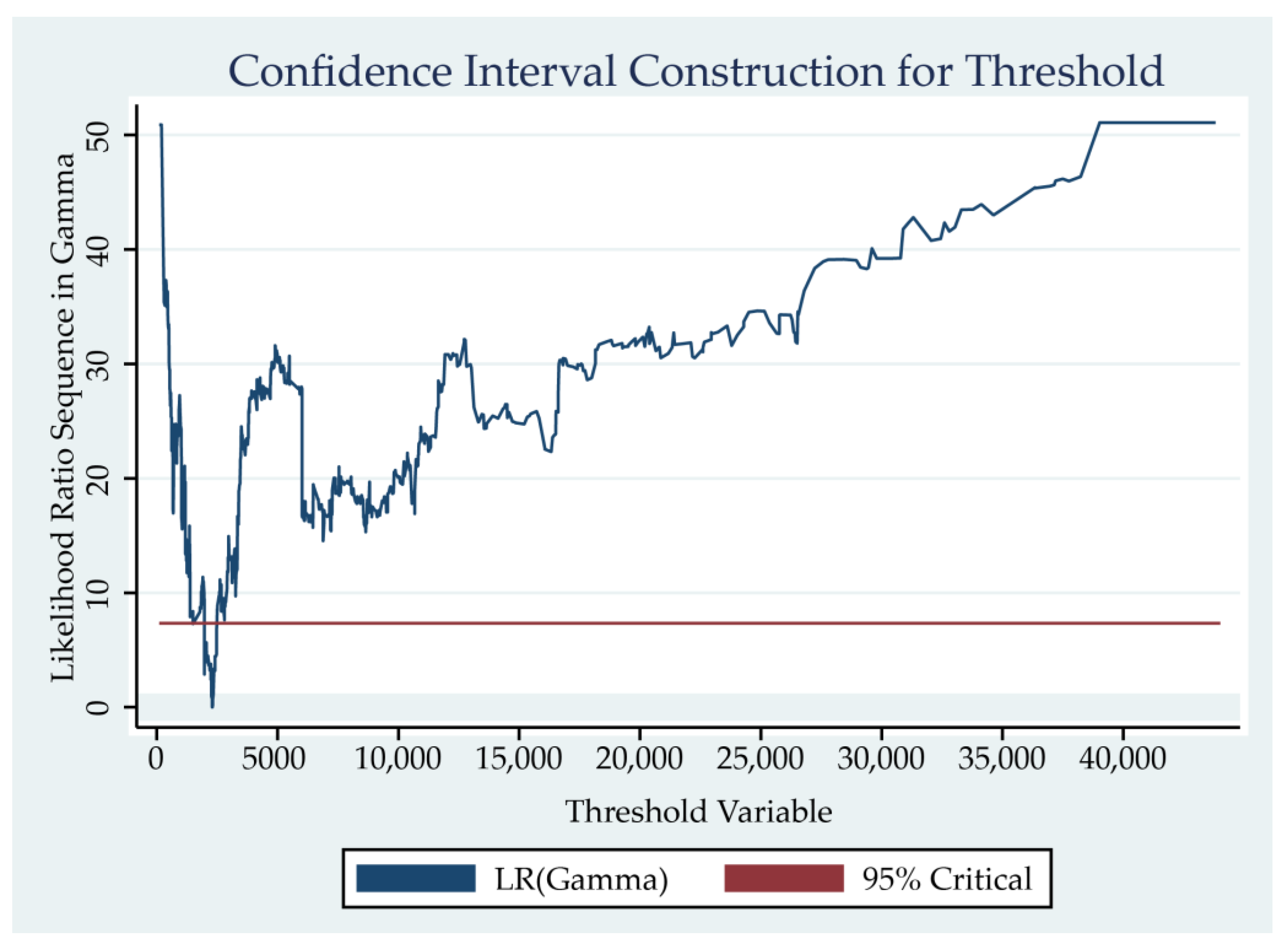
Table 5. Threshold test.
Threshold VariableLM-TestBootstrap
p-Value
Threshold Value0.95 Confidence
Interval
BA45.3460.0002323[1744, 2484]
Table 6. Threshold regression results.
LN(BEC)BA < Threshold ValueBA > Threshold Value
βpβp
GSD−0.323 0.010 −0.177 0.050
LN(RD)0.666 0.000 0.180 0.014
LN(POI)−0.013 0.694 0.067 0.004
LN(CDD)0.719 0.000 1.079 0.000
LN(BA)2.280 0.000 1.254 0.000
LN(TE)0.023 0.864 −0.056 0.386
YEAR1−0.318 0.007 −0.160 0.020
YEAR2−0.127 0.419 −0.186 0.019
YEAR3−0.479 0.020 −0.123 0.225
YEAR4−2.222 0.085 −2.602 0.015
CONSTANT−0.323 0.010 −0.177 0.050
Note: By taking 2015 as a reference, YEAR1 refers to whether the year was 2016. If yes, it is 1; otherwise, it is 0. YEAR2 refers to whether the year was 2017, YEAR3 refers to whether the year was 2018, and YEAR4 refers to whether the year was 2019.
Disclaimer/Publisher’s Note: The statements, opinions and data contained in all publications are solely those of the individual author(s) and contributor(s) and not of MDPI and/or the editor(s). MDPI and/or the editor(s) disclaim responsibility for any injury to people or property resulting from any ideas, methods, instructions or products referred to in the content.

