Article

Carbon Emission Composition and Carbon Reduction Potential of Coastal Villages under Low-Carbon Background

1
School of Architecture, Tianjin University, Tianjin 300072, China
2
School of Architecture, Tsinghua University, Beijing 100190, China
3
College of Design and Engineering, National University of Singapore, Singapore 117566, Singapore
*
Authors to whom correspondence should be addressed.
These authors contributed equally to this work and share first authorship.
Buildings 2023, 13(12), 2925; https://doi.org/10.3390/buildings13122925
Submission received: 1 October 2023 / Revised: 21 November 2023 / Accepted: 22 November 2023 / Published: 23 November 2023

Abstract

:
Rural buildings have high optimization potential as a major source of carbon emissions. However, the current research on carbon reduction in rural buildings is rough and lacks categorization and geographic studies. Coastal villages are more economically developed than other types of villages and have greater potential for energy saving. Therefore, this study takes the carbon emission data of buildings and life in 409 villages in typical coastal provinces of China as the basis and proposes optimization strategies for carbon reduction in coastal village buildings via cluster analysis and correlation analysis. The results show that the carbon emission characteristics of coastal villages can be categorized into three scenarios: for scenario 1, villages, their population, and village cultivated area are the core influencing factors of carbon emission, while for scenarios 2 and 3, the most central influencing factors are coal and electricity consumption. Therefore, different types of villages should be guided differently when studying carbon sinks and carbon emission projections in coastal villages. This study aims to establish a low-carbon performance quality assessment and optimization pathway for coastal villages, and the analysis of carbon emission influencing factors and the assessment and optimization provide theoretical support and quantitative methods for the optimization of carbon reduction in villages.

1. Introduction

As the global climate crisis intensifies, carbon-reducing development in various industries is becoming the mainstream of academic research in various countries [1]. The Sixth Assessment Report (AR6) of the United Nations Intergovernmental Panel on Climate Change (IPCC), released on 27 February 2023, is the most up-to-date and comprehensive analysis of global climate change, which builds on the Fifth Assessment Report (AR5), comprehensively evaluates the current status and trends of changes in the global climate system, and further clarifies the strong linkages between human activities and global warming [2]. As the most basic form of settlement in human society, the countryside has attracted a lot of attention; rural settlements carry a series of important functions, such as production and life of rural residents, and are the concentrated manifestation of the intensity of human activities in the process of human-land relations and social development in the rural areas [3]. On 21 January 2023, the World Bank released data showing that the global rural population reached 4526.1 million people in 2022, accounting for more than half of the world’s total population and that the building sector in rural areas has more potential for carbon reduction [4]. Therefore, the study of rural carbon emissions is particularly important and necessary. China is a typical agricultural country, and according to the data from the 2022 China Statistical Yearbook, the area of various types of land in the countryside accounts for 94.7% of the country’s total area. The energy consumption of rural buildings accounts for 24.5% of the total energy consumption of buildings in China, and the carbon emission scale accounts for about 35% of the total carbon emission scale in China, so the countryside has more space and potential for carbon reduction than the cities [5].
Production and life in rural areas are important components of carbon emission drivers, and the buildings that carry these behaviors are even more important carbon emission spaces. Accompanied by the gradual advance of global urbanization and the gradual transfer of high-carbon functions from cities to lower-level villages on the basis of urban building clusters and urban building clusters, the carbon emissions from villages have gradually become an important part of carbon emissions from human activities in recent years [6]. Relevant studies show that there are differences in energy consumption and industrial layout in villages of different regions, which leads to the different composition of carbon emissions, but according to the currently available papers, it can be found that scholars have carried out some calculations, evaluations and predictions of single-factor carbon sources and sinks in rural production activities, such as building operation [7], agricultural production [8], animal husbandry [9], photovoltaic carbon sinks, and so on [10]. The results have proved that rural buildings are important carriers of carbon emissions in production and life, and the energy use and production activities generated therein are one of the main sources of global greenhouse gases [11,12]. Due to its characteristics, rural development often lags behind urban development [13], and the same is true for energy use. Compared with cities that have basically completed the electrical transformation, rural buildings are more efficient than urban buildings. Most rural areas in developing countries use a mix of energy sources, namely, electricity, natural gas, coal, and biomass energy. The carbon emissions of coal and biomass energy are several times the carbon emissions of electric energy and natural gas, but the energy efficiency generated is hardly equal to that of electric energy and natural gas [14]. In the industrial field, there is no agriculture and animal husbandry in cities and more service industries, which also proves that there is a large space for optimizing the industrial proportion in rural areas [15]. To emphasize the carbon emissions of the rural system, it is necessary to clarify its calculation boundaries and influencing factors. Due to the difficulty of obtaining data in the field and the impracticality of conducting a census, few researchers in the relevant fields have studied the systematic carbon emissions in rural areas. The current research results mainly focus on the following aspects: Firstly, carbon emissions are closely related to agricultural production activities, such as agricultural waste treatment, and the impacts of carbon emissions on the rural system [16], agricultural production inputs [17] and land use and use conversion [18]. Secondly, they analyzed the carbon emissions of different types of agricultural production activities, such as animal husbandry [19,20] and agriculture [21,22]; the literature demonstrates that both have a large share of carbon emissions and need to be matched by a systematic optimization scheme. From the perspective of rural households, in some rural areas, residents are resistant to the implementation of rural energy efficiency and emission reduction policies due to a lack of basic knowledge about carbon emissions and climate change [23]. This can lead to a lack of understanding of the environmental impact of their energy use habits and, thus, a failure to realize the importance of reducing carbon emissions [24]. For different geographical characteristics of the village carbon emissions, differences in the current study are still relatively small; interdisciplinary analysis of the problem can often be better to dig into the problem of the status quo, and rural low-carbon planning from the perspective of geography can be analyzed from a new perspective to obtain the differences between different geographic villages and explore the impact of the relationship between them so that the optimization strategy can be more clearly sorted out. From the relevant literature, it is known that the types of villages with different geographical characteristics generally include four types, i.e., plain villages [25], mountain villages [26], coastal villages [27], and plateau villages [28,29]. Among them, coastal villages have advantages compared with other villages due to their geographical location, convenient transportation, foreign trade activities, good economic foundation, relatively complete infrastructure, and prerequisites for low-carbon optimization, so they have better carbon emission reduction potential [30].
By summarizing and combing the existing academic achievements, it is not difficult to see that there are few relevant studies on rural carbon emission differences from the perspective of geographical differences, and there is a great space for relevant studies on rural carbon emission structure, influence mechanism, carbon reduction potential, and other fields in coastal areas. Therefore, in this paper, using field research and remote sensing data summarization of coastal villages, the core influencing elements of carbon emission in three types of villages were extracted, and the influencing mechanism between each element and carbon emission was established. We finally summarize the research system for the analysis of the composition of the carbon emission and the potential of carbon reduction in geographically different villages and put forward the characteristics of the carbon emission of coastal villages in line with the study area and the carbon emission patterns of different scenarios. It also proposes the carbon emission characteristics of coastal villages and the carbon emission composition patterns of different scenarios for different types of villages in the study area.
This paper provides practical ideas for the follow-up research on rural carbon emissions in coastal areas and proves with examples that coastal villages have good low-carbon research prospects and high demand. Secondly, the research ideas of other rural areas with different geographical conditions can be extracted from the study of coastal rural areas, which greatly expands the research space of rural carbon emission structure. Finally, by proposing low-carbon optimization suggestions for different types of coastal villages, this paper can provide a better theoretical basis for policy formulation for professional researchers related to urban and rural planning.

2. Materials and Methods
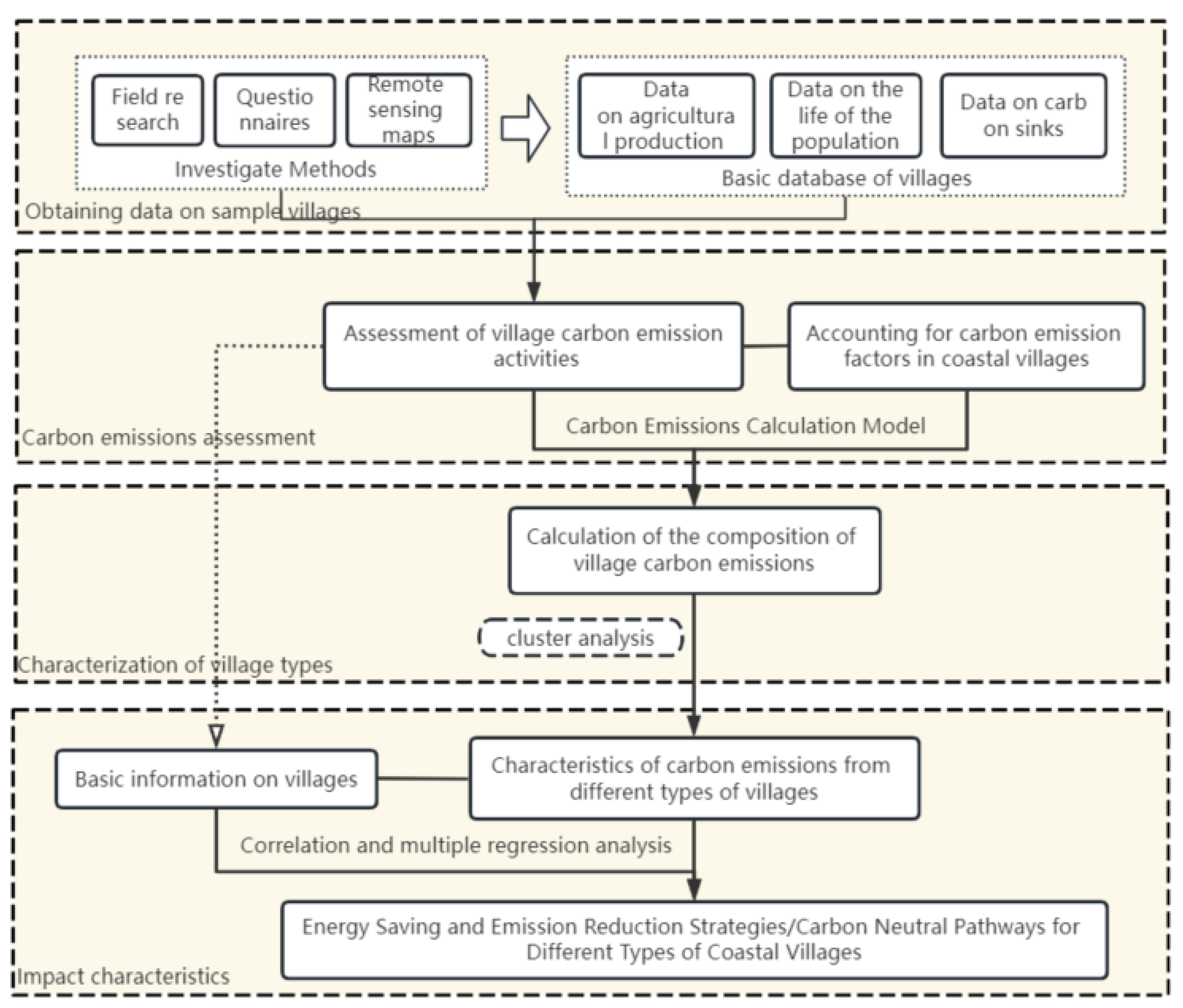
2.1. Outline

The purpose of this paper is to analyze the carbon emission characteristic composition and carbon reduction potential of coastal villages; the acquisition of carbon emission composition needs to be carried out via the design of the questionnaire based on the current existing relevant research foundation; this paper determines the questionnaire content via the expert interviews and the literature combing [31,32,33] and determines the overall research steps using the result orientation based on the carbon emission characterization method of coastal villages; the research is specifically carried out in four steps, as shown in Figure 1.
The first step is to obtain real sample data on coastal villages; this stage is to obtain the basic data of rural carbon emission activities in villages via field research, questionnaires, remote sensing maps, and other ways, including the data on residents’ life, agricultural production, carbon sinks, and so on. Please refer to the table of contents for the part of the questionnaire survey. The main interviewees should be residents living in the target villages all year round, and the methods are mainly online filling and interviewing so as to prevent the tension of the interviewees from affecting the survey results.
Secondly, the different carbon emissions of all sample villages are measured and processed via the carbon emission calculation model to obtain the carbon emission data of different segments. Before the data processing, the rationality of the data is basically judged, and the data are screened in advance.
In the third step, the carbon emission results of different villages are classified by clustering algorithm, the samples affecting the quality of the data are analyzed and processed, and the type of carbon emission and the number of samples of the villages to be finally analyzed are determined according to the elbow analysis and so on.
Finally, correlation analysis and multiple regression analysis are carried out according to the results of the calculation and analysis in the third step and the basic situation of the villages to analyze the characteristics of the samples, the structure of carbon emissions, and the carbon reduction potential of different villages and ultimately form the carbon reduction paths of different types of villages.

2.2. Questionnaire Preparation and Data Collection

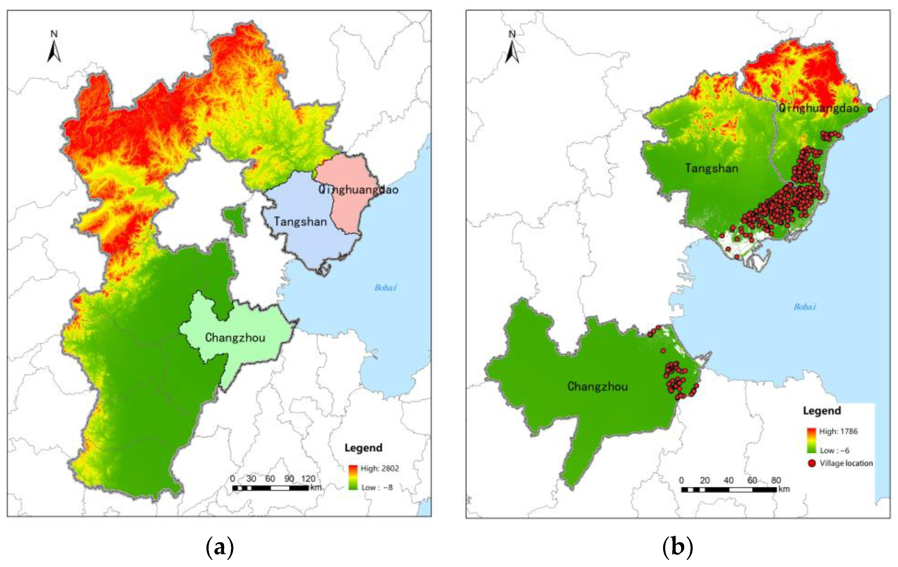
2.2.1. Sample Selection

Hebei, one of the most rural provinces in China, can provide a large number of case samples for the research and practice of low-carbon rural communities because of its large rural area, long coastline, more coastal villages than in other regions, and more developed economy within the coverage of China’s national urban agglomeration, the Beijing–Tianjin–Hebei urban agglomeration. The coastal villages are characterized by diversified industrial patterns and wide distributional differences, which make the villages in the coastal areas of Hebei highly representative. Hebei Province is located in the north of the Yellow River and is an important winter heating area. Therefore, the types of rural energy use in this area are more comprehensive than those in the south of China. In addition, since the population density of China is higher in the south than in the north, the rural areas in the north tend to have more farmland and animal husbandry area, so there is more room for research adjustment, so it has higher research value. In order to better describe the location relationship of the research samples in a wide-area environment and to show the relationship between the selection of rural sites and the coastline, it can be seen from Figure 2a,b that the locations of the research samples selected in this paper are the coastal parts of eastern Hebei Province, mainly the selection of villages along the coastline, and their main ground locations are relatively flat and open. It is far away from the hilly areas and plateau areas in the north.
Firstly, the villages in Hebei Province were screened and Z-standardized to reduce the influence of extreme values. The processing method is commonly used in the analysis of data with different data types and large differences, and the data can be simplified for subsequent analysis [33]. The items, such as the number of populations, cultivated land area, number of livestock, and energy consumption in the raw data, were calculated by the following Formula (1):
Z i , j = x i , j x j ¯ σ j
In the formula, Z i , j is the Z-score for the jth parameter of the i-th data set; x i , j is the jth parameter value for the i-th data set, and x j ¯ , σ j are the overall mean and standard deviation of the jth parameter, respectively.
The Z-score characterizes the degree of deviation of the data from the overall mean, and the larger the absolute value of the Z-score, the farther the data is from the whole [34,35]. In this paper, the data are screened according to the absolute value of Z-score less than 3. A small number of villages that are too large or too small to be representative in terms of area or population are excluded, and about 409 village samples are selected. The screened 409 samples have a regular spatial distribution in Hebei Province, involving many areas of the three coastal cities in Hebei Province, which basically represent the overall situation of coastal villages in Hebei Province. Secondly, because the qualification of this paper has been determined as coastal, the production and lifestyle of China’s coastal villages have certain similarities, and the selected villages can also represent other coastal villages in China to a certain extent. The distribution of the number of households in the 409 samples is shown in Figure 3, with 75% of the villages in the range from 84 to 420 households, of which the largest number of villages is around 200 households, and 90% of the cultivated area is less than 2000 acres.

2.2.2. Data Collection

The data sources involved in this study are mainly statistical data and field research. Statistical data mainly come from the China Statistical Yearbook, China Rural Statistical Yearbook, Hebei Provincial Environmental Quality Bulletin, and online statistical databases [36,37,38]. Empirical data include both relevant departmental visits and field research. The departmental visits mainly collect data from the administrative departments where villages are located, and we designed a questionnaire about their energy consumption based on daily life, energy consumption practices, and the existing literature on villages in coastal areas of China [39]. Based on the results of the preliminary survey and interviews, the questionnaire was improved to obtain the final scale, which can be divided into three parts: behavioral and cognitive survey; spatial pattern survey; and energy consumption survey. (1) Behavioral and cognitive survey via the questionnaire and interview, the villagers’ daily production, life content to record, according to the combing of the related literature; human behavior habits often have a greater impact on building energy consumption and carbon emissions [40]; so, using the acquisition of the behavior habits of rural residents, we can better determine the characteristics of the energy use of the entire countryside as well as a more accurate rural carbon emissions data [41]; (2) Spatial pattern survey, mainly to clarify the unit boundaries of rural carbon emissions, related research shows that in some countryside areas, which are closer to the city compared to the countryside far away from the city, the energy structure has a greater difference; via the determination of the travel characteristics of the rural population and the public transportation configuration it can be easy to access the spatial pattern of the countryside to analyze the impact of spatial pattern on the rural carbon emissions; (3) Energy use and consumption survey: the use of questionnaires and administrative visits in the form of a combination of forms, access to the corresponding energy consumption data help access the whole countryside energy use, including life and production behavior, via the villagers and the whole countryside; at the same time, access to the data can play a mutual corroboration to improve the authenticity of the data for the subsequent data screening to provide a basis for comparison. The energy consumption data emission factor data refer to the IPCC Guidelines for National Greenhouse Gas Inventories [42] and China Energy Statistical Yearbook [43], etc., and the electric power part is based on the Baseline Emission Factor of China Regional Power Grid [44], which finally obtains the data of carbon emission activities of 409 villages.

2.3. Data Acquisition Method

The sources of rural GHG emissions can be roughly divided into two categories: one is the GHG emissions from agricultural production activities, for coastal villages are mainly planting and animal husbandry due to geographic location and the surrounding market environment and other factors. In the case of this paper, coastal aquaculture is mainly for the industrial clusters, which basically does not exist in the case of individual aquaculture, not the villagers’ family production, so this paper does not discuss aquaculture; The other category is the greenhouse gas emissions generated in the course of residents’ living behaviors, including energy, transportation, and waste disposal, and the greenhouse gases involved are mainly carbon dioxide, methane, and nitrous oxide, whose corresponding 100-year GWP values are 1, 27, and 273, respectively [42]. Broadly speaking, animal husbandry belongs to one of the agricultural types; for convenience of expression, agriculture in this paper only refers to the planting industry, while animal husbandry is listed separately. As for the calculation method, there are two main methods for carbon emission calculation, i.e., the emission factor method and the mass balance method, of which the mass balance method is more complicated and not applicable to the use of this paper, so this paper adopts the carbon emission factor method, which is relatively common and highly recognized, for the calculation, in which the data of the carbon emission factor can be obtained from the relevant policy documents in China.

2.3.1. Calculation of Carbon Emissions from Residential Living

Carbon emissions from residential living mainly include the following three parts: carbon emissions from building operations; carbon emissions from transportation; and carbon emissions from domestic waste and sewage discharges. With regard to building operation energy consumption, this includes daily use energy consumption and heating and cooling energy consumption, which varies from region to region in terms of energy consumption and demand. According to the actual situation, household energy use is generally electricity, natural gas, gas, biomass, etc. The specific types can be obtained by checking the IPCC Guidelines for National Greenhouse Gas Inventories. For transportation, carbon emission needs to be adjusted according to the type of car and oil usage, and for those who use public transportation, it should also be treated according to the public transportation carbon emission factor. The average household vehicle ownership can be calculated via on-site research or based on the number of durable goods held by rural residents in the statistical yearbook of each province as a reference.

2.3.2. Calculation of Carbon Emissions from Residential Production

For carbon emissions from residential production, this paper focuses on production behaviors that take place in rural areas, mainly including agricultural production and animal breeding behaviors. For agricultural production, the main sources of carbon emissions include the following: (1) carbon emissions caused by agricultural material inputs, including fertilizers, pesticides, agricultural films, agricultural diesel, irrigation, plowing, and other agricultural material inputs generated by carbon emissions; (2) Carbon emissions from the growth and development of rice; (3) Carbon emissions from enteric fermentation and manure management in ruminant farming. By adding data on factors related to plant carbon sinks as appropriate, the formula for calculating carbon emissions from the agricultural sector can be summarized as follows:
C A = E A g r + E A q u E t
In the formula, EAgr is total crop GHG emissions (tCO2-eq/a); EAqu is total GHG emissions for breeding (tCO2e/a); Et is carbon reduction for plant carbon sinks (tCO2-eq). The values of the relevant parameters are shown in the Table A1 of Appendix B [45].
For the carbon emission calculation of the livestock farming component, carbon emission accounting is mainly carried out by counting the equivalent amount of carbon dioxide of methane and nitrous oxide gases produced by livestock in the rearing process. The specific formulas are as follows, and the specific correlation coefficients are shown in Table A2 of Appendix B [13].
E C H 4 , A H = T i × E F C H 4 , i × β i
E N 2 O , A H = T i × E F N 2 O , i × β i
Based on the above calculations of the three areas of village carbon emissions, the formula for calculating overall village carbon emissions can be summarized as follows:
C N = C + C A + E w C R e n Δ C A C T U A L , t
In the formula, C N is total rural carbon emissions (tCO2-eq/a); C is total carbon emissions from the living sector (tCO2-eq/a); C A is total carbon emissions from agriculture(tCO2-eq/AP); E w is total carbon emissions from transportation (tCO2-eq); C R e n is renewable energy system carbon sink (tCO2e); Δ C A C T U A L , t is the total reduction in village carbon sink in year t (tCO2-eq/a).

2.4. Data Analysis

Due to the geographical conditions, population size, and living habits of each village, agricultural production, animal breeding, waste and sewage generation, and energy consumption are different, showing different greenhouse gas emission characteristics. With the help of SPSS (version 20) and Python platform, the equivalent carbon dioxide emissions of each pathway in the research villages are used as parameters for clustering analysis, and the clustering mean can reflect the emission characteristics of different types of villages. The k-mean clustering algorithm is a kind of division algorithm with a known number of clustering categories. It is very typical of distance-based clustering algorithms, which use distance as an evaluation index of similarity [46]. The prerequisite for this algorithm to achieve effective clustering is to determine the accurate clustering center, which is generally determined by randomly defining k-data points as the initial clustering center for clustering and then calculating the center value of the k-class clusters as the new clustering center to recluster, and repeating the process until the clustering criterion function converges [47,48]. In general, when the minimization squared error E of the clusters after clustering is smaller, it means that the data samples within each type of clusters are closer to the cluster mean vector, and the degree of similarity of the samples within the clusters is higher [49].
Single-factor linear regression analysis [31] can be used to screen whether there is a significantly close correlation between each impact factor in the three categories and the total village discounted carbon emissions. The resulting p-value < 0.05 indicates that the influence factor has a significant correlation with the total discounted carbon emissions of villages under this category; otherwise, it does not constitute a significant correlation. The test results obtained via linear regression analysis will be used as the basis for multiple regression analysis of this variable. In this paper, the total village population (IV01), area of cultivated land (IV02), number of pig breeds (IV03), number of cattle breeds (IV04), number of sheep breeds (IV05), domestic waste (IV06), average annual electricity consumption (IV07), average annual gas consumption (IV08), average annual coal consumption (IV09), and average annual biomass (IV10) in three different clusters are used, as well as 10 parameters as influence factors and the total discounted carbon emissions (DV01) of the village as assessment indicators using SPSS for linear regression analysis to analyze the influence of the residential environment of the village on the village carbon emissions.
Multiple regression analysis is a method of statistical analysis in which one of the variables in a correlation is set as the dependent variable, and one or more of the other variables are considered independent variables, establishing a mathematical model quantitative relationship between multiple independent variables and dependent variables. Multiple regression analysis is a method of statistical analysis in which one of the variables in a correlation is set as the dependent variable, and one or more of the other variables are considered independent variables, establishing a mathematical model quantitative relationship between multiple independent variables and dependent variables. The statistical analysis method of mathematical modeling is a quantitative relationship equation [50]. In this paper, the influence of village basic information parameters on carbon emissions is quantified by fitting the quantitative relationship equation between multiple village basic information parameters (independent variables) and village total converted carbon emissions (dependent variable), and the general multiple regression analysis results are expressed as follows:
Y = b 0 + b 1 X 1 + b 2 X 2 + + b n X n + ε
In the formula, Y is the dependent variable; b 0 is the unstandardized coefficients for constants; b 1 , b 2 b n is the unstandardized coefficient of the independent variable; X 1 , X 2 X n is the 1, 2⋯ nth independent variable; ε is the error value.
In the process of multiple regression analysis, there are several indicators to focus on. The first is the unstandardized coefficient value, which will be used directly in constructing the regression equation. The second is the standardized coefficient Beta value because there may be differences in the nature, unit scale, order of magnitude, and other attributes between the independent variables entered in this study; the standardized coefficient Beta value can eliminate the differences in the attributes of multiple independent variables and intuitively compare the degree of influence of each independent variable on the dependent variable, and the order of the size of this item is the order of the degree of influence of multiple independent variables on the dependent variables. Finally, we need to pay attention to the test indicators of the regression model, which is used to determine whether the output of the regression analysis results is reasonable. The test of multiple regression analysis is mainly judged from four perspectives: t-test; goodness-of-fit test; covariance test; and residual test. In this paper, the parameters with a strong correlation with village carbon emissions are screened out by correlation analysis as independent variables, and the total converted carbon emissions of the villages are used as dependent variables for regression analysis. The calculation method adopts the step-by-step method, which can exclude the independent variables that do not satisfy the t-test one by one by setting the screening range of the significance p-value to ensure that the output parameters of the villages are all the parameters that satisfy the t-test.

3. Results

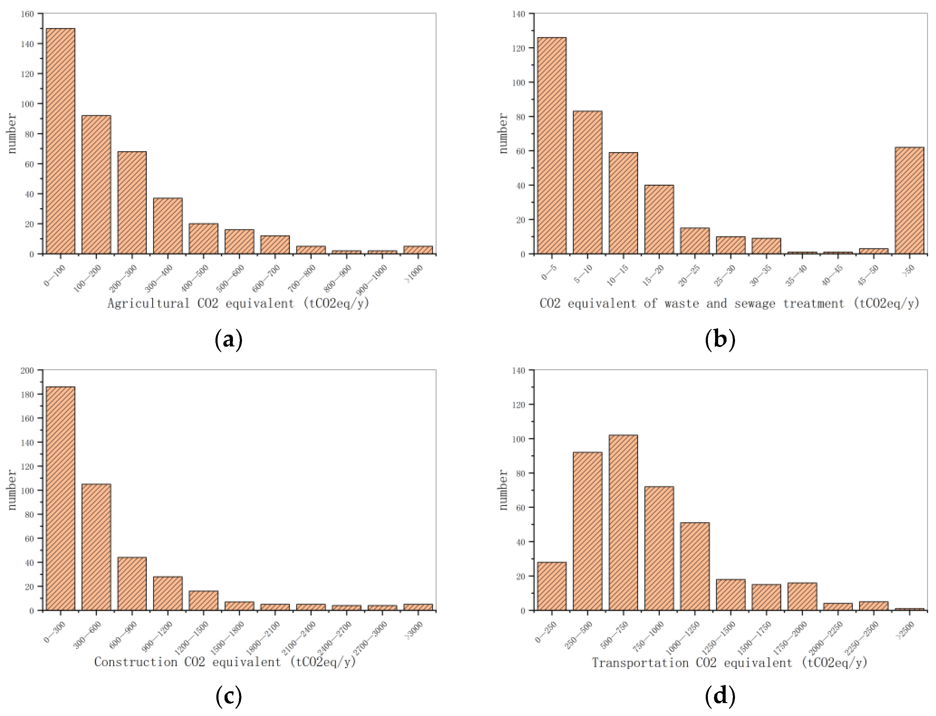
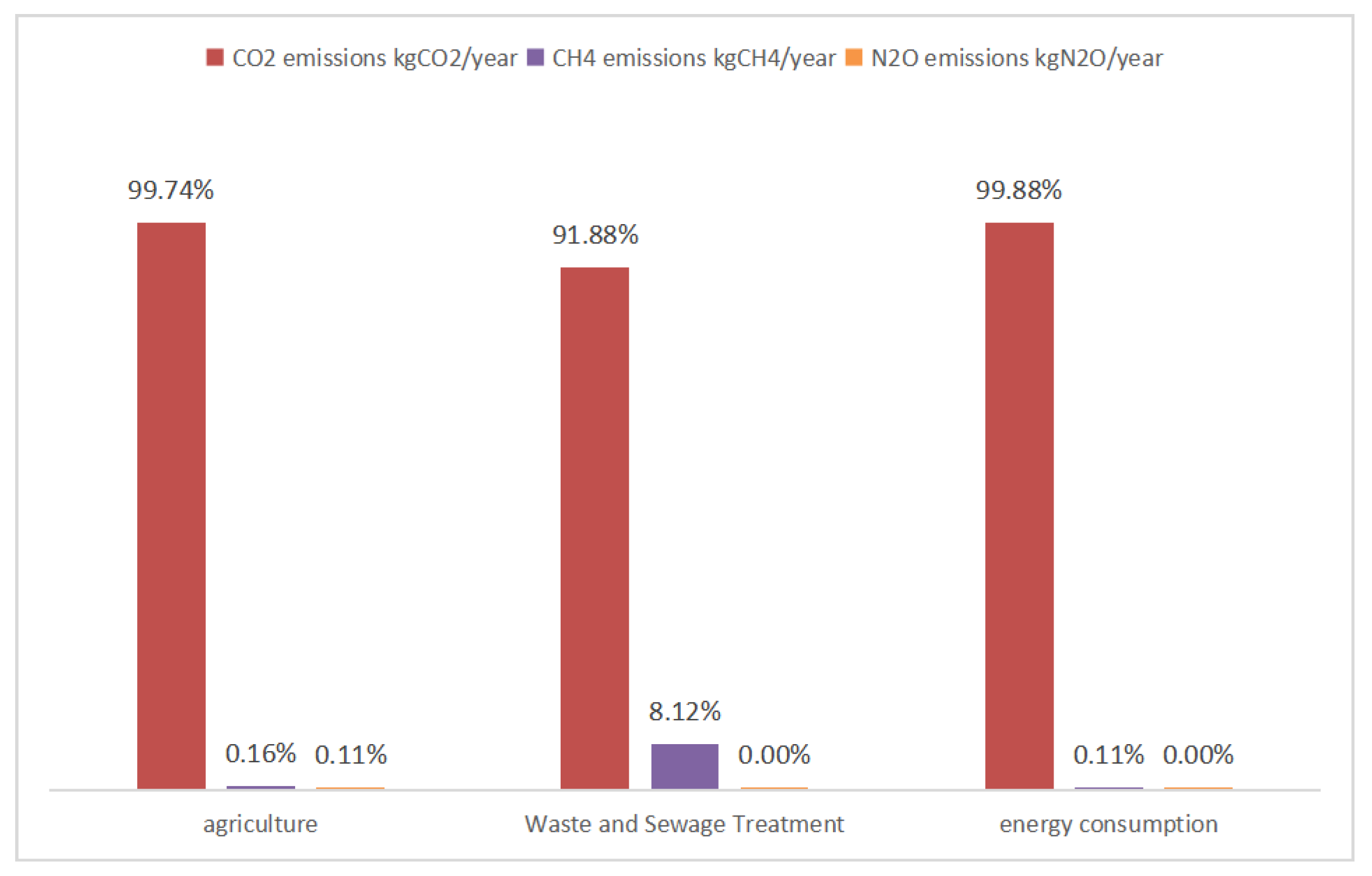
3.1. Carbon Emission Calculation Results

The distribution of equivalent carbon dioxide (CO2e) emissions from agricultural production, waste and sewage treatment, residential life, and transportation is shown in Figure 4. It can be seen that the sample of agricultural carbon emissions is mainly concentrated between 0 and 100, which is lower compared with residential life and transportation but higher than the carbon emissions generated by domestic waste and sewage. Residential living carbon emissions are more concentrated; annual carbon emissions are mainly 300 tons of CO2e, but there are also quantities higher than 300 tons of CO2e. This shows that the coastal areas of the countryside have better economic development, and the energy structure is relatively advanced. For waste and sewage, due to the current centralized treatment mode being quite mature, the treatment method is basically fixed for landfill and incineration, so the carbon emissions of domestic waste and sewage are mainly from the degradation of carbon emissions within the calculation boundary of the countryside, and the amount of carbon emissions in the samples is also relatively centralized, which is related to the economic conditions. If the economic conditions are better, domestic waste and sewage will be higher as well. This is related to their economic conditions, as better economic conditions tend to produce higher amounts of domestic waste and sewage [51,52]. From the histogram of emissions, transportation GHG emissions show a significant normal distribution. The GHG emissions from waste disposal are at a low value. Agriculture and residential GHG emissions also show significant differences.

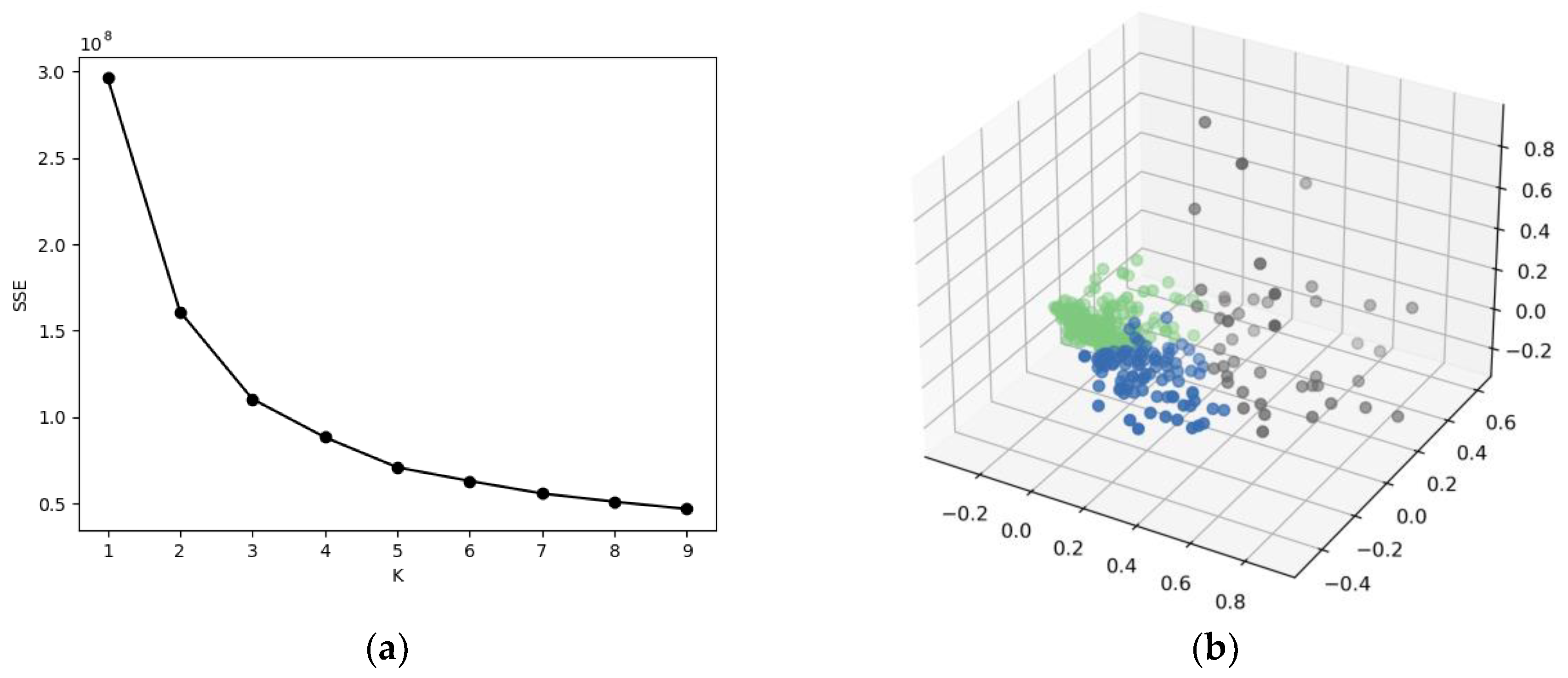
3.2. K-Mean Cluster Analysis

Since the number of clusters could not be determined in advance, the “elbow rule” was used to determine the optimal number of clusters by comparing the sample error squared and SSE under different numbers of clusters [40]. The inflection points where the SSE decreases significantly are selected as the optimal number of classifications. In this study, the change in the error sum of squares with the number of clusters is shown in Figure 5a, which shows that when k = 3, the error sum of squares decreases at a significant “inflection point”, so this paper divides the sample data into three categories. According to the elbow rule, the research village data are divided into three major categories after dimensionality reduction clustering, and their data distribution is shown in Figure 5b, using k-means clustering to cluster the three major parts of the data distribution in three-dimensional space to present the characteristics of aggregation, indicating that according to the elbow rule clustering data classification effect is good, and it has a clear degree of differentiation and statistical classification significance.
The number of samples in each clustering center and each type is shown in Table 1. In terms of emissions by pathway in the clustering centers, building energy consumption emissions > transportation emissions > agricultural emissions > waste sewage treatment emissions. Building energy consumption and waste sewage emissions are highest in type 1 and lowest in type 2, while agricultural and transportation emissions are highest in type 3 and lowest in type 2.
From the basic case information of the villages in the clustering center, type 2 is the general pattern of coastal villages, which belongs to the lower level in terms of population and cultivated land, and type 3 of carbon emission is mainly the high-intensity pattern of coastal villages, which is in the higher level of coastal villages in terms of population, cultivated land, animal husbandry, and all kinds of living and production modes, etc. Type 1 is relatively similar to type 2 in terms of basic information about the villages and production and life, but it belongs to the more extreme level; in terms of energy consumption, it is higher than the other two types, which is an extreme level. The distribution of the mean values of basic rural information by type is shown in Figure 6. It is clear that type 2 is at a lower level in all aspects, while type 1 is closer to type 2 in terms of population and number of farms but significantly higher than the other two types in all aspects of energy consumption, except for arable land, which is lower than the average of type 2.
In the greenhouse gas calculation method proposed earlier, except for the influence of the number of animal breeds on the amount of nitrogen input to farmland, the influencing factors of each emission pathway do not intersect, and the structure of greenhouse gases in the same emission pathway is basically the same. On average, the main GHG emitted from agricultural production is carbon dioxide, accounting for 99.74%, which comes from the use of fertilizers, pesticides, agricultural films, and other types of agricultural materials, followed by nitrous oxide emissions caused by nitrogen input from chemical fertilizers, manure, straw, and other nitrogen; due to the small area of rice cultivation in Hebei, the smallest proportion of GHGs in the agricultural sector is methane, and it mainly comes from agricultural waste-water. Waste and sewage treatment greenhouse gases are dominated by methane, accounting for 91.88% of the total, originating from landfills and domestic sewage, followed by carbon dioxide and nitrous oxide, originating from waste incineration and domestic sewage, respectively. Energy consumption emitted 99.88% carbon dioxide. The exact percentage is shown in Figure 7.

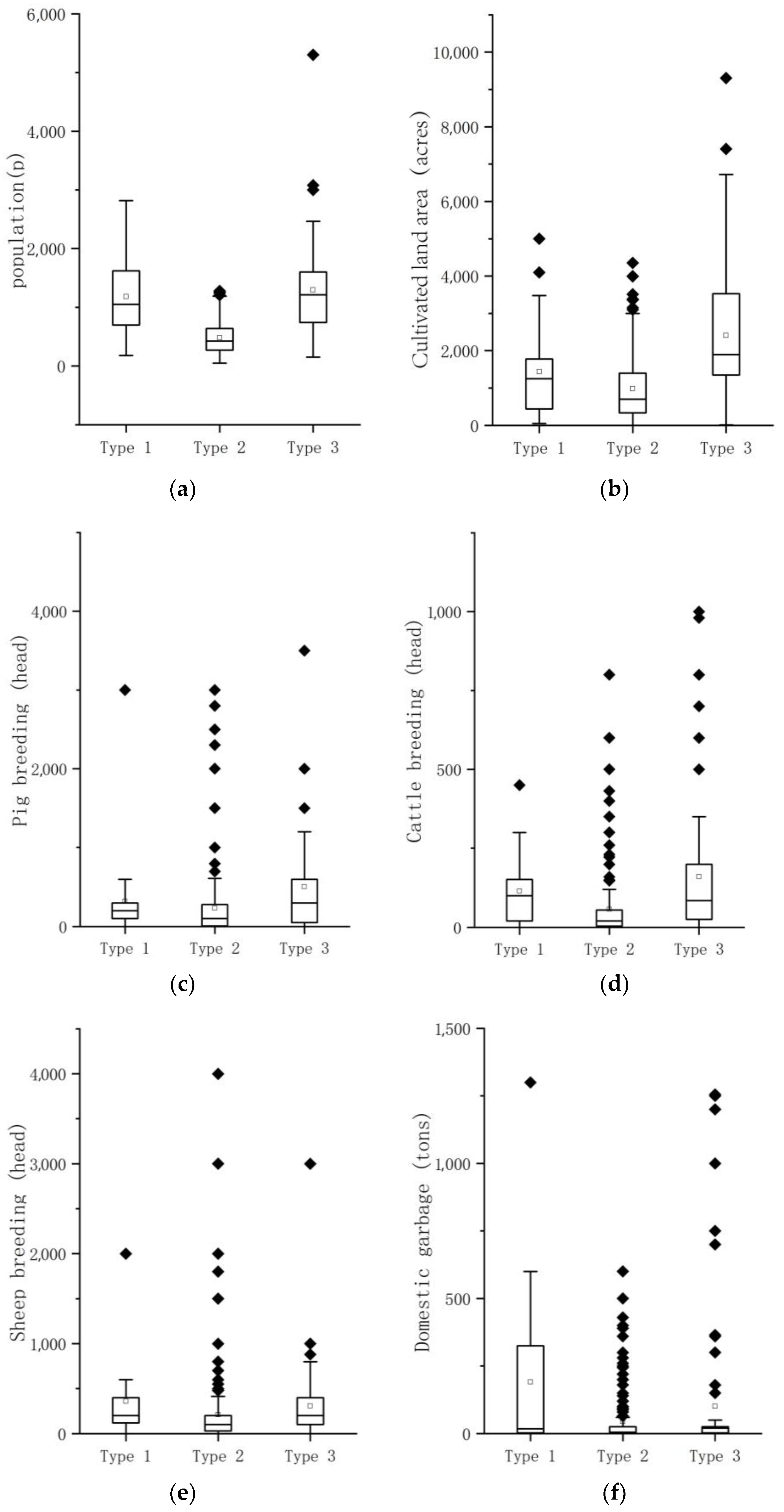
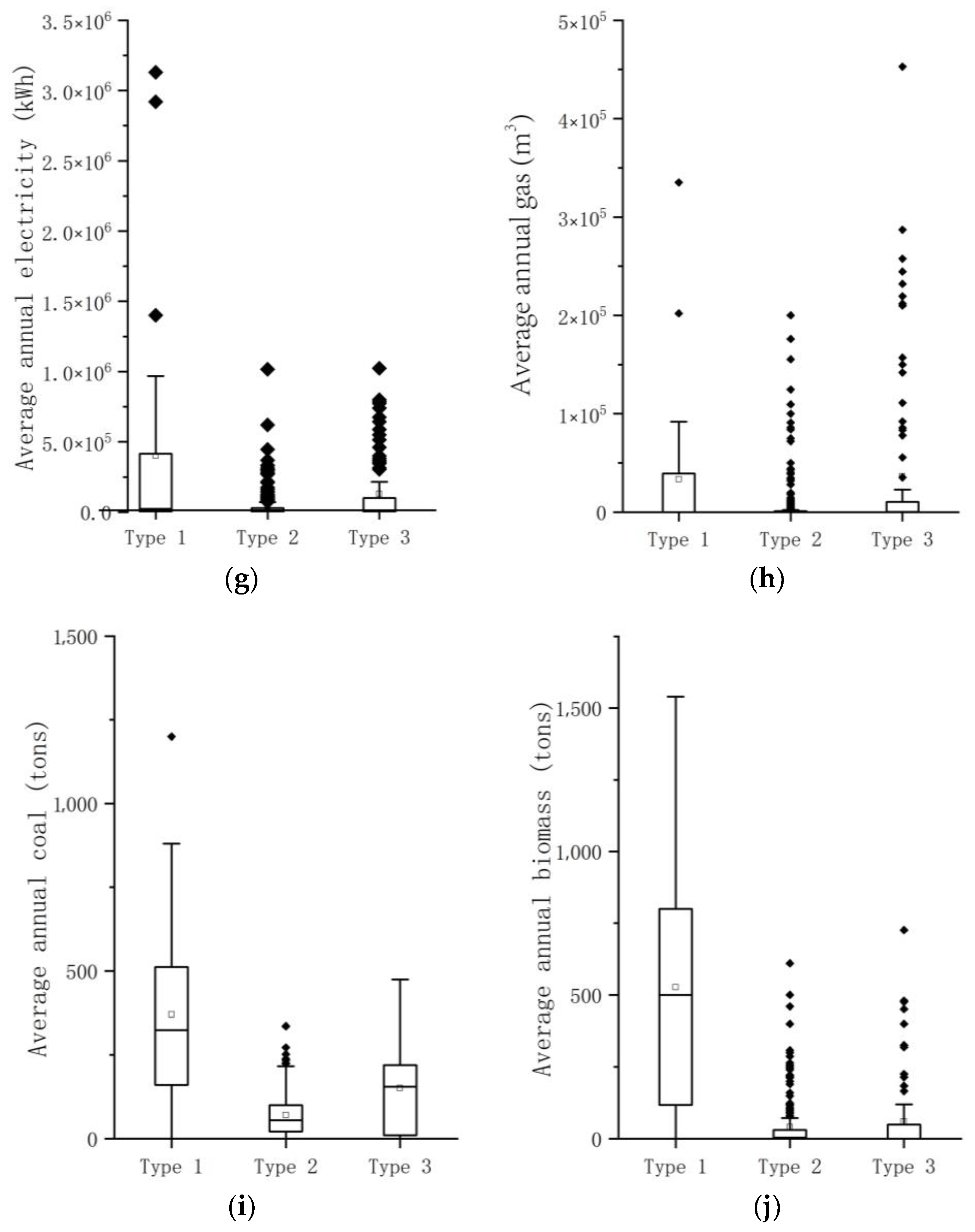
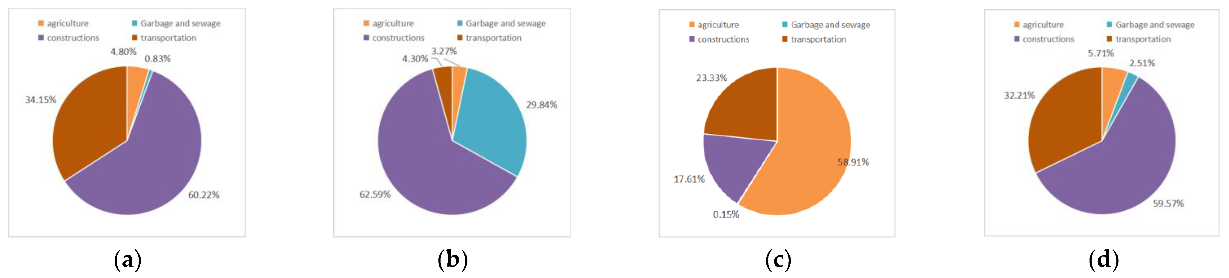
3.2.1. Type 1 Rural Emission Characteristics

Type I rural accounts for only 8.21% of the total but has the highest overall level of rural population, arable land, and energy consumption of the three types, as well as the highest level of agriculture, energy consumption, and total equivalent carbon emissions, which represent the extremes of the research villages. In terms of the sources of greenhouse gas emissions from various categories, carbon dioxide mainly comes from building energy consumption, accounting for 60.22%, followed by agricultural production, accounting for 34.15%, and waste and sewage, accounting for a lower percentage. Methane mainly comes from building energy consumption, accounting for 62.59%, followed by waste and sewage treatment, accounting for 29.84%; emissions from transportation and agricultural production are low. Nitrous oxide emissions are mainly from agricultural production with 58.91%, followed by transportation and energy consumption and less than 1% are from waste sewage. The main source of total equivalent CO2 emissions considering GWP is energy consumption at 59.57%, followed by transportation at 32.21%, agriculture at 5.71%, and waste sewage emissions with the lowest share. The specific shares are shown in Figure 8.

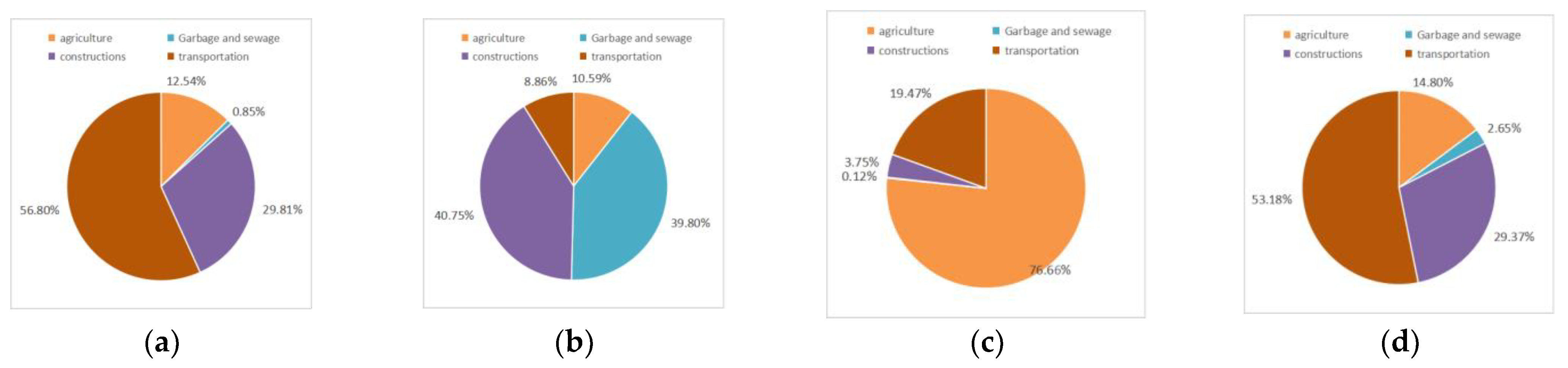
3.2.2. Type 2 Rural Emission Characteristics

The proportion of rural areas in Type 2 is 70.90%, which is at a lower level in terms of population, arable land, energy, and equivalent carbon dioxide emissions by pathway, and represents the average level of greenhouse gas emissions in the research area. From the point of view of the proportion of emissions of various types of greenhouse gases by different pathways, the proportion of emissions of various types of greenhouse gases by pathways in Type 2 differs from that of Type 1 in a more obvious way. The share of carbon dioxide emissions from transportation reaches 56.80%; the share of building energy consumption decreases to 29.81%, and the share of agriculture and waste disposal is basically the same as Type 1. Methane emissions are dominated by building energy consumption and waste disposal, accounting for 40.75% and 39.80%, respectively, followed by transportation and agriculture. Nitrous oxide emissions are mainly from agriculture, with a share of 76.66%, followed by transportation and energy consumption; waste-water treatment has the lowest share. The main source of total equivalent carbon dioxide (TEC) emissions was transportation at 53.18%, followed by building energy consumption at 29.37%, animal husbandry at 14.80%, and waste-water treatment at 2.65%. The detailed percentages are shown in Figure 9.

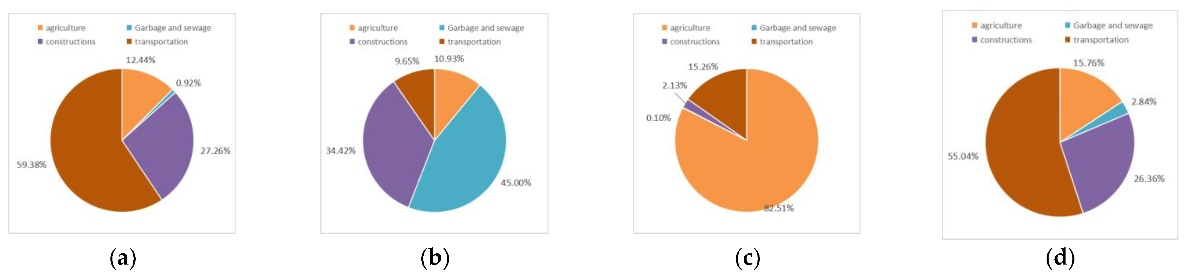
3.2.3. Type 3 Rural Emission Characteristics

Type 3 rural emission characteristic accounts for only 21.7% of the total in terms of population, arable cultivation, livestock feeding, and transportation, and the overall level of agricultural emissions is the highest of the three types; agriculture and energy consumption are also at a high level, representing the medium–high level of the research village. Type 3 rural energy consumption exceeds the other types, and the share of agricultural production emissions in carbon dioxide emissions is 59.38%, while waste and sewage emissions are less than 1%. The share of waste sewage methane emissions reaches 45.5%, exceeding 34.42% of building energy consumption, while transportation and agricultural emissions are tied at 9.65% and 10.93%, respectively. For nitrous oxide emissions, agriculture has the highest share of 82.51%, followed by transportation and energy consumption, and less than 1% for waste sewage treatment. Of the total equivalent of carbon dioxide emissions, transportation emissions accounted for 55.04%, followed by building energy consumption, agriculture, and waste sewage with 26.36%, 15.76%, and 2.84%, respectively. Details of the shares are shown in Figure 10.

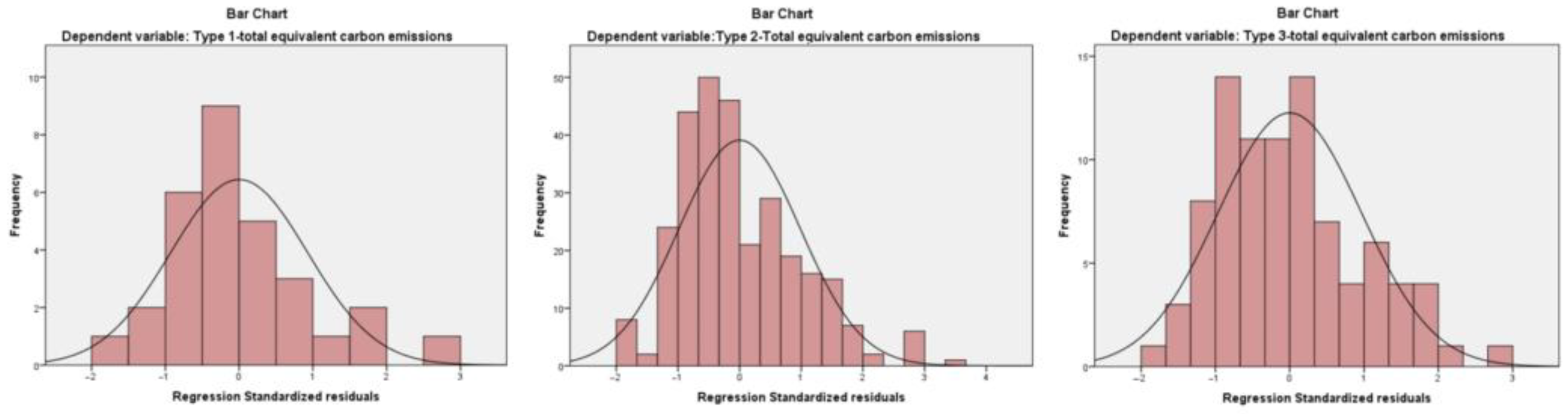
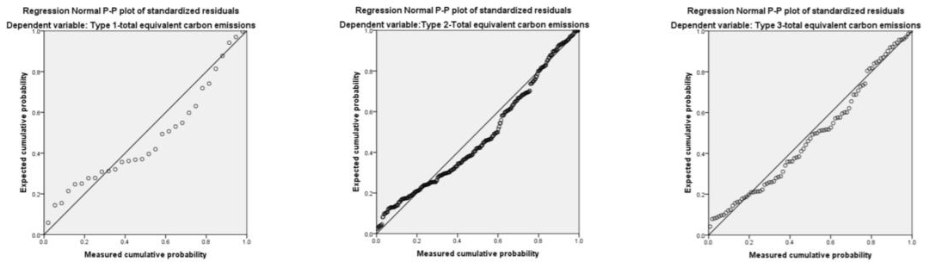
3.3. Results of Linear Regression Analysis and Multiple Regression Analysis for Different Types

For the three village cases mentioned in the previous section, this paper analyzes the linear correlation between the influence shadow of carbon emission and the total carbon emission of the village and screens out the influence parameters with a significant correlation. In different types, the significant correlation factors and the number of factors that affect the total carbon emission of villages are different. The test results of the core factors that have a significant correlation (p < 0.05) with the total amount of converted carbon emissions in the three villages are as follows: The core factors of type 1 were village population (IV01) (p = 0.039 < 0.05), village cultivated land area (IV02) (p = 0.017 < 0.05), annual average utilization of coal consumption (IV09) (p = 0.043 < 0.05), and annual biomass utilization (IV10) (p = 0.027 < 0.05); The second core factors were village population (IV01) (p = 0.041 < 0.05), cultivated land area (IV02) (p = 0.012 < 0.05), cattle breeding (IV04) (p = 0.013 < 0.05), sheep breeding (IV05) (p = 0.026 < 0.05), domestic waste (IV06) (p = 0.013 < 0.05), average annual electricity consumption (IV07) (p = 0.032 < 0.05), average annual coal consumption (IV09) (p = 0.033 < 0.05), and average annual biomass consumption (IV10) (p = 0.006 < 0.05); Population (IV01) (p = 0.008 < 0.05), cultivated land area (IV02) (p = 0.014 < 0.05), domestic waste (IV06) (p = 0.009 < 0.05), average annual gas consumption (IV08) (p = 0.018 < 0.05), average annual coal consumption (IV09) (p = 0.022 < 0.05), and annual biomass use (IV10) (p = 0.026 < 0.05) were significantly correlated with total converted carbon emissions of type 3. In the three types of villages studied, there is a significant correlation between total carbon emissions, village population, and cultivated land area, indicating that the carbon emissions of most of the villages studied are closely related to the village population and cultivated land area.
Linear regression analysis can screen and explain the influence path between village basic information parameters and building energy consumption, but it is difficult to explain the influence relationship with village carbon emissions under the joint effect of multiple basic information parameters, so in order to further quantify the degree of joint influence of basic information on total carbon emissions in the above types of villages, this paper utilizes multivariate regression analysis to explore the influence of the law under the joint influence of each basic information parameter. Based on the results of regression analysis (Table 2), it can be seen that the three types of regression models of type 1, type 2, and type 3 have a goodness-of-fit Ra2 of 0.740, 0.883, and 0.722, respectively, and the goodness-of-fit is greater than 0.5. The degree of goodness-of-fit is better than 0.5, which is statistically significant. The carbon emissions (DV01t1) of type 1 villages are mainly affected by the population (IV01), the area of cultivated land (IV02), the average annual use of coal (IV09), and the average annual use of biomass (IV10), and the regression equation is
DV01t1 = 1.22 × IV01 + 0.254 × IV02 + 1.473 × IV09 + 1.203 × IV10 + 1020.446
Total type 1 equivalent carbon emissions = 1.22 × population + 0.254 × cultivated land area + 1.473 × average annual use of coal + 1.203 × average annual use of biomass 1020.446. From the standardized coefficient Beta value of each influence parameter can be quantified to derive the degree of influence of the respective variable on the dependent variable, the degree of influence of the village information parameter on the carbon emissions of type 1 from largest to smallest for the degree of influence of the state parameter on the energy consumption of the building in the following order of magnitude: the population of the village (0.653) > average annual use of biomass (0.499) > average annual use of coal (0.367) > village cultivated area (0.278). The carbon emissions of type 2 villages (DV01t2) are mainly affected by the number of population (IV01), cultivated area (IV02), cattle breeding (IV04), sheep breeding (IV05), domestic waste (IV06), average annual use of electricity (IV07), average annual use of coal (IV09), and average annual use of biomass (IV10) in a joint manner, and the regression equation is:
DV01t2 = 0.66 × IV01 + 0.175 × IV02 + 0.109 × IV04 + 0.036 × IV05 + 0.526 × IV06 + 0.001 × IV07 + 3.203 × IV09
+ 1.641 × IV10 + 212.314
Total type 2 equivalent carbon emissions = 0.66 × population + 0.175 × cultivated land area + 0.109 × cattle breeding + 0.036 × sheep breeding + 0.526 × domestic waste + 0.001 × average annual use of electricity + 3.203 × average annual use of coal + 1.641 × average annual use of biomass + 212.314. From the standardized coefficients of the respective impact parameters, Beta value can be quantified to derive the degree of influence of the respective variables on the dependent variable; the degree of influence of the village information parameters on type 2 carbon emissions from largest to smallest is the degree of influence of the state parameter on building energy consumption from largest to smallest and it is average annual use of coal (0.439) > village population (0.396) > cultivated land area (0.336) > average annual use of biomass (0.302) > domestic waste (0.173) > average annual electricity use (0.128) > number of sheep breeds (0.078) > number of cattle breeds (0.045). And the carbon emission (DV01t3) of type 3 villages was mainly affected by the population (IV01), cultivated area (IV02), domestic waste (IV06), average annual use of gas (IV08), average annual use of coal (IV09), and average annual use of biomass (IV10), together with the following regression equation:
DV01t3 = 0.29 × IV01 + 0.147 × IV02 + 0.592 × IV06 + 0.002 × IV08 + 2.987 × IV09 + 1.797 × IV10 + 1180.104
Total type 3 equivalent carbon emissions = 0.29 × population + 0.147 × cultivated land area + 0.592 × domestic waste + 0.002 × average annual gas use + 2.987 × average annual coal use +1.797 × average annual use of biomass +1180.104. The standardized coefficient of the Beta value of each influence parameter can be quantified to derive the degree of influence of the respective variables on the dependent variable and the influence of the village information parameter on the type 3 carbon emissions. The degree of influence of the state parameters on building energy consumption from largest to smallest is the average annual coal use (0.572) > cultivated area (0.394) > average annual use of biomass (0.341) > domestic waste (0.317) > village population (0.309) > average annual gas use (0.291).
In order to test the reliability of the results of the above regression equation, it is necessary to carry out the standardized residuals test, which can be judged from the standardized residuals histogram and standardized residuals normal probability plot. From the histogram of standardized residuals (Figure 11), it can be seen that the model residuals of the total carbon emissions of the three types of villages and the basic information parameters of the villages are more in line with the normal distribution of the relationship; from the normal probability of the standardized residuals (Figure 12), it can also be seen that the samples are distributed on both sides of the diagonal of the first quadrant, which meets the validation criteria of normal distribution, indicating that the regression equation meets the requirements of residual tests; in summary, it can be decided that the regression model has a certain degree of reliability. The test analysis can determine whether the results of the regression model have a certain degree of reliability.

4. Discussion

Rural carbon emissions as a hot spot direction in recent years have gradually been paid in-depth attention by various disciplines, although despite significant results [31,53,54], there is a lack of multidisciplinary cooperation. The development of low-carbon villages has positive significance for protecting the environment, promoting sustainable development, and narrowing the gap between urban and rural areas [55]. As mentioned in the introduction, the analysis of rural energy issues in China has been booming [56], and rural energy consumption, as a major source of China’s greenhouse gas emissions, is an important aspect of reducing China’s carbon emissions [57]. A low-carbon countryside is an important means to develop a low-carbon economy and realize energy saving and emission reduction [58]. Economic growth and population contribute positively to carbon emissions in the low-carbon countryside, generating more carbon dioxide emissions, while technological advances, changes in the agricultural structure, and changes in the national industrial structure have negative impacts, which have a positive effect on emission reduction and carbon emission reduction [9], and a positive effect on emission reduction and carbon reduction has been obtained in the previous study of the impact of economic structure on carbon emissions [59]. Similar conclusions were obtained, while adjusting the agricultural structure and agricultural technology has reduced greenhouse gas emissions compared to traditional farms that grow maize without the use of mineral fertilizers [60,61].
However, there are obvious differences in the development of low-carbon villages under different geographic characteristics, which also provides a broad research prospect for related studies [62]. As climate change has attracted more and more attention, countries around the globe are taking action to mitigate the impacts of climate change [63]. Among them, carbon peaking and carbon neutrality have become one of the main ways to achieve global emission reduction targets. Traditional carbon emission assessment methods only consider the energy consumption of enterprises and households while ignoring the impact of geographical features on carbon emissions. Therefore, when assessing the carbon emissions of low-carbon villages, it is necessary to consider the impact of geographical characteristics and adapt to the stage of development in order to better serve the rural grassroots in realizing energy transition and upgrading. The differences in carbon emissions of villages with different geographic characteristics are not the same [64]; relevant studies analyze the influencing factors of energy and emissions of rural households via case studies [65,66], but the current study still lacks the study of the basic characteristics of villages.
In this study, we have conducted an in-depth exploration of the potential and methods of energy saving and emission reduction in coastal villages. Using a large amount of research data, the carbon emissions of 409 villages along the coast of China were accounted for. Via cluster analysis, the villages’ carbon emissions were classified into three types. Via linear regression analysis and multiple regression analyses, the influence of the basic information of the villages on the carbon emissions of the villages is analyzed and discussed, and different energy-saving and emission-reduction strategies are proposed for different types of villages, which provide references for the coastal village planning and rural governance for the purpose of energy saving. The three different types of villages divided by the basic characteristics of villages in this study have different carbon emission pathways, but in the overall situation, the main carbon emission comes from the construction of buildings, and there are some types in which agriculture accounts for a large proportion, which is consistent with previous studies [67], but the importance of agriculture and animal husbandry is different from the results of the latest study [68]; the reason for that lies in the difference in geographical location and the cash crop structure of the villages. From the numerical point of view, there is an obvious gap between the main part of the buildings and traffic stations of the village sample of type 1 and the emission of agricultural and domestic sewage. Although the proportion of construction and transportation for the village sample of type 2 is also high, the proportion of agriculture is relatively balanced. From the characteristics of high carbon emissions from construction operations and transportation, it can be seen that the third-type villages belong to the villages with good economic levels. Compared with the characteristics of the first type of village with high carbon emissions in the building part and the third type of village with high carbon emissions in the traffic part, the type 2 villages are more moderate in carbon emissions, which is related to the fact that the rural residents are generally more economical and simpler, and the economic situation is generally worse than that of the first and third type of villages. The second type of villages exactly reflects the characteristics of most Chinese villages, which meet the basic living conditions but have not yet reached the level of well-being, which proves that the villages in the second category are more common than those in the first and third categories. This is also the reason why the number of samples in the second category is the largest. It can also be seen from the clustering characteristics that economic conditions tend to push rural carbon emissions to a higher level, which is caused by rural residents’ pursuit of a better quality of life [69].
Since the scope of this study mainly focuses on the coastal villages in China and the research data are concentrated on 409 villages along the coast of China, the conclusions of this study lack some applicability to coastal villages in other regions outside China. However, in the coastal villages in northern China, the carbon emission structure of the villages is similar due to similar living habits and industrial policies. Therefore, the conclusions of this study mainly guide the energy-saving and emission-reduction strategies of coastal villages in Hebei Province and also have certain application scenarios for coastal villages in northern China. In addition to this, when analyzing the carbon emission problems of coastal villages in this study, in order to make the carbon emission data of the villages more representative and not be interfered with by a small number of extremes, a small number of villages have been screened for special carbon emissions, such as special industries or special machinery, according to the relevant literature. However, since this study is mainly based on most ordinary coastal villages to explore carbon emission saving and emission reduction methods, extreme villages are not the object of study, which may cause some errors. At the same time, due to the characteristics of China’s national conditions, the current research results may not be applicable to coastal villages in other countries. The results may change and become more accurate.

5. Conclusions

Based on the Provincial Greenhouse Gas Emission Inventory Guidelines and IPCC Carbon Emission Inventory Methodology, this paper has systematically sorted out the calculation methods of greenhouse gas emissions in rural areas and accounted for the greenhouse gas emissions of 409 effective research villages. Based on the calculation results, the k-mean clustering algorithm was used to analyze the structure of GHG emissions in the research villages, and the following conclusions were drawn:
Rural greenhouse gas emission pathways can be divided into four parts: agricultural production; waste and sewage treatment; energy consumption; and transportation consumption. Based on the equivalent carbon dioxide emissions of each pathway, the rural villages investigated in this paper can be divided into three types, and there are differences in the industrial structure, living habits, energy consumption, and other aspects of different types of villages, so the structure of greenhouse gas emissions is different. There are differences in population size and industrial structure among the three types of rural areas, and the total equivalent carbon emissions are dominated by energy consumption. Therefore, rural areas, especially villages with high energy consumption levels, should pay attention to energy conservation and energy structure adjustment and promote the improvement in energy efficiency and the use of renewable energy. In agriculture, scientific management should be promoted to avoid excessive use of chemical fertilizers and pesticides and to reduce carbon dioxide and nitrous oxide emissions. Transportation emissions should be optimized by optimizing the road structure and enhancing the popularity of green new energy transportation. For waste and sewage, the level of collection and treatment should be improved, the proportion of solid waste incineration should be increased, and high methane and nitrous oxide emissions should be reduced. In addition to low-carbon optimization in rural areas, the economic benefits of rural development should also be ensured. For low-income villages with high carbon emissions, more energy-efficient ways should be considered to improve energy efficiency, and the planting area of high-yield crops should be increased by reducing the proportion of low-energy efficiency facilities to achieve carbon reduction and income increase. For low-income villages with moderate carbon emissions, economic benefits should be given priority, and the growth rate of carbon emissions should be slowed down in the process of economic development. There should be a way to balance development worth exploring.
Rural greenhouse gas emissions are closely related to the basic parameters of villages, and the carbon emissions of the three types of village cases derived from the cluster analysis are affected by different basic parameters, and the degree of influence varies. The linear regression analysis between the basic parameters of each type of village and the total converted carbon emissions of the village and the results of multiple regression analysis found that the carbon emissions of the village and the population and cultivated area of the village have a significant impact path, and for type 1 villages, the village population and the cultivated area of the villages are the core influencing factors, and the core influencing factor for types 2 and 3 is the average annual coal consumption. So, when studying its carbon sinks and carbon emissions prediction, we should focus on taking into account its carbon emission and population forecasting. Therefore, when studying their carbon sinks and carbon emission forecasts, we should focus on population and cultivated land area, appropriately return farmland to forests, build green areas to enhance carbon sequestration and carbon reduction capacity, reduce the use of coal in construction and domestic waste, and apply new types of energy and waste control to reduce carbon emissions.
Based on a large amount of village basic information and village greenhouse gas emissions research data, this paper uses k-mean clustering to classify villages into three categories, analyzes their respective greenhouse gas emissions and emission pathways, and uses linear regression analysis and multiple regression analysis to analyze the influence factors and influence degree of village carbon emissions under the simultaneous influence of village basic parameters and multi-parameters. This paper establishes a low-carbon performance quality assessment and optimization path for coastal villages, and the analysis of carbon emission influencing factors and assessment and optimization provide theoretical support and quantitative methods for village carbon reduction and optimization and provide design guidelines for rural carbon reduction and sequestration and green low-carbon rural construction.
In the process of this study, the quantitative impact relationship between the existing impact factors and rural carbon emissions can be determined according to the currently identified impact factors. The follow-up research plan is proposed here to further investigate and explore the deeper influencing factors of carbon emissions, and to promote the research and analysis of other regional rural areas. Finally, a set of low-carbon emission reduction strategies and optimization paths are proposed that can be applied to all types of villages.

Author Contributions

Conceptualization, Z.Y., G.Q. and Z.L.; methodology, Z.Y., G.Q. and Z.L.; software, Y.W. and L.R.; validation, Z.Y., G.Q. and Z.L.; formal analysis, Z.Y. and Z.L.; investigation, Z.Y.; resources, Z.Y.; data curation, Y.W.; writing—original draft preparation, Z.Y., G.Q. and Z.L.; writing—review and editing, Z.Y., G.Q. and Z.L.; visualization, G.Q. and L.R.; supervision, G.Q. and Z.L.; project administration, Z.Y.; funding acquisition, Z.Y. All authors have read and agreed to the published version of the manuscript.

Funding

This research was funded by National Natural Science Foundation of China, grant number 52078265.

Data Availability Statement

Data will be made available on request. The data are not publicly available due to privacy.

Acknowledgments

The authors would like to thank the research participants for assisting in this study.

Conflicts of Interest

The authors declare no conflict of interest.

Appendix A

Appendix A.1. Village Energy Structure and Industry Survey Questionnaire

Appendix A.1.1. Basic Information of the Village

  • Home City
    • Plain cities: Hengshui; Langfang; Xingtai;
    • Mountain cities: Shijiazhuang; Baoding; Handan;
    • Coastal cities: Tangshan; Qinhuangdao; Cangzhou;
    • Plateau cities: Chengde; and Zhangjiakou.
  • Village Name:
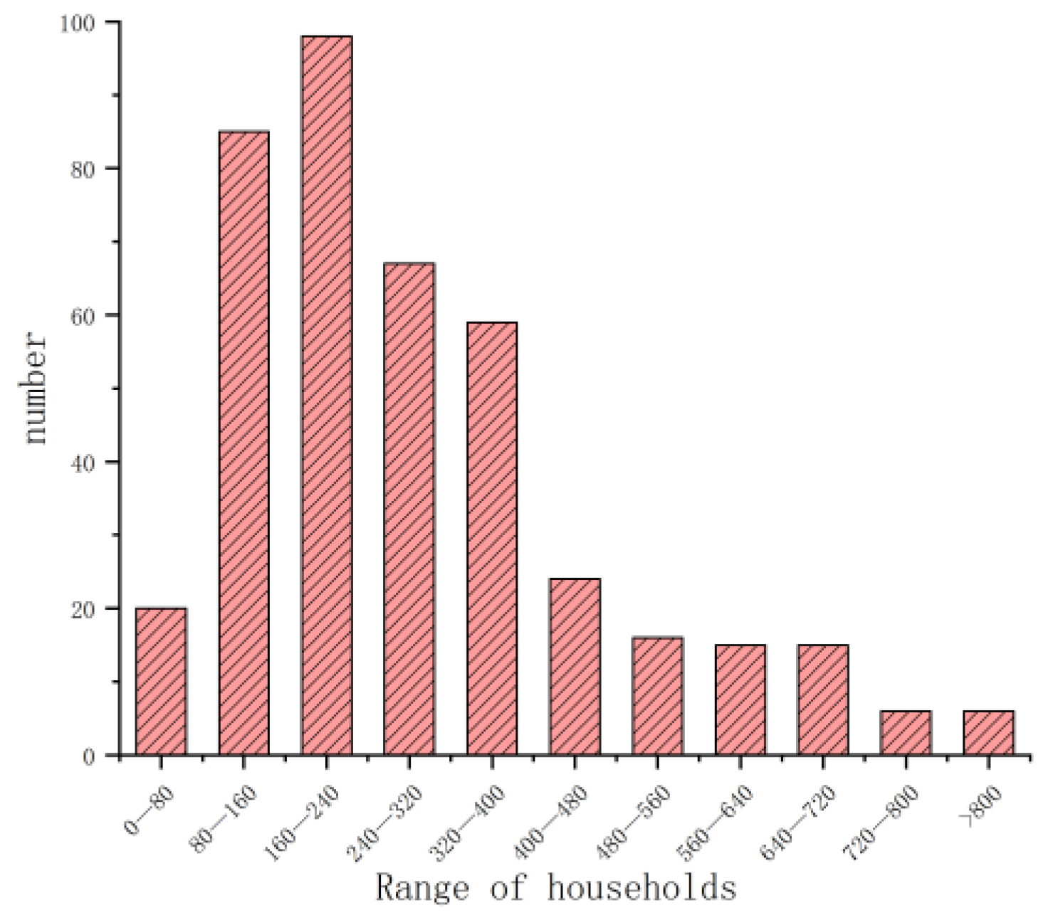
  • Number of households:
  • Resident population:
  • Main industries in the village:
    • Farming;
    • Forestry;
    • Fishery;
    • Livestock;
    • Tourism services;
    • Industrial.
  • Annual output value of the village:

Appendix A.1.2. Village Land Type and Area Statistics

7.
Village Land Type and Area
Area (mu)
Village area
Residential land area
Infrastructure area
Landscaped green area (artificial landscape)
Natural forest area
Area of cultivated land for agriculture (agricultural crop cultivation)
Water Area (Aquaculture)
Pasture area
Forestry, orchard planting area (nursery, etc.)

Appendix A.1.3. Investigation of Domestic Waste

8.
Frequency of garbage removal in the village:
  • Daily;
  • Three days;
  • One week;
  • Two weeks;
  • One month.
9.
Total amount of domestic waste (ton)

Appendix A.1.4. Investigation of the Agricultural Situation in the Village Area

10.
Name of the main crops planted in the village
Planting Area (mu)
Corn
Wheat
Hulled oats
Rice
Cotton
Vegetables and fruits
Other
11.
Whether to use combine harvesters for harvesting [multiple choice] *
  • Yes;
  • No.
12.
Number of public transport trunk lines in villages

Appendix A.1.5. Investigation of Energy Use in Villages

13.
Village Annual Energy Consumption Summary
20182019202020212022
Power (kwh)
Natural gas (cubic meters, including pipeline gas, etc.)
Coal (ton, clean coal, general bulk coal, honeycomb briquette, etc.)
Biomass (tons, firewood, biomass pellets, etc.)
14.
Village New Energy Usage and 2022 Output
Annual Production (kwh/Year; GJ/Year)
Photoelectric resources
Wind power resources
Geothermal energy resources
Hydropower resources
15.
Supplement: Total Number of Livestock in Village Animal Husbandry
Quantity (Head)
Pig
Cattle
Sheep

Appendix B

Table A1. Parameters for calculating CO2 emissions from cultivation [42].
Carbon SourceAverage
Consumption per Mu
kg/Acre
CO2 Emission FactorCO2 Emissions per Acre
kg/Acre
Nitrogen Fertilizer8.296.3852.90
Phosphorus fertilizer1.840.611.11
Potash Fertilizer1.730.440.76
Compound Fertilizer11.692.4828.93
Pesticide0.4518.098.10
Agricultural Film0.0818.991.60
Agricultural Diesel11.582.1725.17
Irrigation--4.85
Total--123.42
Note: This paper is based on the characteristics of China’s agriculture; using the collation of the agricultural film is not a one-time consumption; public documents show that in 2020, the recovery rate of agricultural film in Hebei Province has reached 90.17%, so the consumption of agricultural film in the table is 9.83% of the amount used in the year.
Table A2. Parameters for calculating GHG emissions from livestock (Adapted with permission from Ref. [45]. 2021, Masson-Delmotte, et al.).
Animal SpeciesIntestinal CH4 Emission Factor
kg/p/Year
Manure CH4
Emission Factor
kg/p/Year
Manure N2O
Emission Factor
kg/p/Year
pig1.003.1200.227
Cattle78.605.1401.320
sheep8.550.1600.093
Note: The cattle-related emission factors in the table take the average values for dairy and non-dairy cattle, and the sheep-related emission factors take the average values for goats and sheep.

References

  1. Mikhaylov, A.; Moiseev, N.; Aleshin, K.; Burkhardt, T. Global climate change and greenhouse effect. Entrep. Sustain. Issues 2020, 7, 2897–2913. [Google Scholar] [CrossRef] [PubMed]
  2. Kikstra, J.S.; Nicholls, Z.R.J.; Smith, C.J.; Lewis, J.; Lamboll, R.D.; Byers, E.; Sandstad, M.; Meinshausen, M.; Gidden, M.J.; Rogelj, J.; et al. The IPCC Sixth Assessment Report WGIII climate assessment of mitigation pathways: From emissions to global temperatures. Geosci. Model Dev. 2022, 15, 9075–9109. [Google Scholar] [CrossRef]
  3. Yong, C. Basic Concepts in the Study of Rural Settlement Ecology. Rural. Eco-Environ. 2002, 18, 54–57. [Google Scholar]
  4. Liu, Y.; Wu, S. The path and challenges of China’s carbon peak and carbon neutrality. J. Clean. Prod. 2020, 277, 124045. [Google Scholar]
  5. Li, X.; Du, J.; Long, H. A comparative study of Chinese and foreign green development from the perspective of mapping knowledge domains. Sustainability 2018, 10, 4357. [Google Scholar] [CrossRef]
  6. O’Neill, B.C.; Zigova, K. Global demographic trends and future carbon emissions. Proc. Natl. Acad. Sci. USA 2010, 107, 17521–17526. [Google Scholar] [CrossRef]
  7. Deng, Q.; Zhang, S.; Shan, M.; Li, J. Research on Envelope Thermal Performance of Ultra-Low Energy Rural Residential Buildings in China. Sustainability 2023, 15, 6931. [Google Scholar] [CrossRef]
  8. Yang, T.; Huang, X.; Wang, Y.; Li, H.; Guo, L. Dynamic Linkages among Climate Change, Mechanization and Agricultural Carbon Emissions in Rural China. Int. J. Environ. Res. Public Health 2022, 19, 14508. [Google Scholar] [CrossRef]
  9. Dai, X.; Wu, X.; Chen, Y.; He, Y.; Wang, F.; Liu, Y. Real Drivers and Spatial Characteristics of CO2 Emissions from Animal Husbandry: A Regional Empirical Study of China. Agriculture 2022, 12, 510. [Google Scholar] [CrossRef]
  10. Li, Z.; Zhang, C.; Yu, Z.; Zhang, H.; Jiang, H. Deep Learning Method for Evaluating Photovoltaic Potential of Rural Land Use Types. Sustainability 2023, 15, 10798. [Google Scholar] [CrossRef]
  11. Yu, Z.; Wang, Y.; Zhao, B.; Li, Z.; Hao, Q. Research on Carbon Emission Structure and Model in Low-Carbon Rural Areas: Bibliometric Analysis. Sustainability 2023, 15, 12353. [Google Scholar] [CrossRef]
  12. Hu, Q.; Zhang, T.; Jiao, Z.; Duan, Y.; Dewancker, B.J.; Gao, W. How does industrial transformation enhance the development of coastal fishing villages: Lessons learned from different transformation models in Qingdao, China. Ocean Coast. Manag. 2023, 235, 106470. [Google Scholar] [CrossRef]
  13. Zhang, H.; Li, S. Carbon emissions’ spatial-temporal heterogeneity and identification from rural energy consumption in China. J. Environ. Manag. 2022, 304, 114286. [Google Scholar] [CrossRef]
  14. Zen, I.S.; Al-Amin, A.Q.; Alam, M.M.; Doberstein, B. Magnitudes of households’ carbon footprint in Iskandar Malaysia: Policy implications for sustainable development. J. Clean. Prod. 2021, 315, 128042. [Google Scholar] [CrossRef]
  15. Nematchoua, M.K.; Sadeghi, M.; Reiter, S. Strategies and scenarios to reduce energy consumption and CO2 emission in the urban, rural and sustainable neighbourhoods. J. Sustain. Cities Soc. 2021, 72, 103053. [Google Scholar] [CrossRef]
  16. Yrjälä, K.; Ramakrishnan, M.; Salo, E. Agricultural waste streams as resource in circular economy for biochar production towards carbon neutrality. J. Curr. Opin. Environ. Sci. Health 2022, 26, 100339. [Google Scholar] [CrossRef]
  17. Ashayeri, M.S.; Khaledian, M.R.; Kavoosi-Kalashami, M.; Rezaei, M. Evaluation of energy balance and greenhouse gas emissions in rice cultivation in Guilan province, northern Iran. J. Paddy Water Environ. 2020, 18, 261–272. [Google Scholar] [CrossRef]
  18. No, J.L.; Erb, K.H.; Matej, S.; Magerl, A.; Gingrich, S. Socio-ecological drivers of long-term ecosystem carbon stock trend: An assessment with the LUCCA model of the French case. J. Anthr. 2021, 33, 100275. [Google Scholar]
  19. Li, M.; Liu, S.; Sun, Y.; Liu, Y. Agriculture and animal husbandry increased carbon footprint on the Qinghai-Tibet Plateau during past three decades. J. Clean. Prod. 2021, 278, 123963. [Google Scholar] [CrossRef]
  20. Menghistu, H.T.; Zenebe Abraha, A.; Mawcha, G.T.; Tesfay, G.; Mersha, T.T.; Redda, Y.T. Greenhouse gas emission and mitigation potential from livestock production in the drylands of Northern Ethiopia. J. Carbon Manag. 2021, 12, 289–306. [Google Scholar] [CrossRef]
  21. Kusumawati, S.A. The Dynamic of Carbon Dioxide (CO2) Emission and Land Coverage on Intercropping System on Oil Palm Replanting Area. J. Oil Palm Res. 2020, 32, 267–277. [Google Scholar] [CrossRef]
  22. Adame, M.F.; Brown, C.J.; Bejarano, M.; Herrera-Silveira, J.A.; Ezcurra, P.; Kauffman, J.B.; Birdsey, R. The undervalued contribution of mangrove protection in Mexico to carbon emission targets. J. Conserv. Lett. 2018, 11, 12445. [Google Scholar] [CrossRef]
  23. Yu, J.; Huang, Y. The Analysis of Correlation between Urban Residents Behavior and Low-carbon Economic Development. Energy Procedia 2011, 5, 1762–1767. [Google Scholar]
  24. Lin, A.; Lou, J.; Yue, R. Study on Residents’ Perception of Low-Carbon Policy and Its Influence on Low-Carbon Behavior Intention. In Sustainability in Energy and Buildings 2022 (SEB 2022); Smart Innovation, Systems and Technologies; Littlewood, J., Howlett, R.J., Jain, L.C., Eds.; Springer: Singapore, 2023; Volume 336. [Google Scholar] [CrossRef]
  25. Zhang, Y.; Tian, J.; Shen, Z.; Wang, W.; Ni, H.; Liu, S.; Cao, J. Emission Characteristics of PM2.5 and Trace Gases from Household Wood Burning in Guanzhong Plain, Northwest China. Aerosol Sci. Eng. 2018, 2, 130–140. [Google Scholar] [CrossRef]
  26. Um, D.-B. Configuring Legitimate Blue Carbon Rights for Coastal Fishing Villages Based on Forestry Carbon MRV. J. Coast. Res. 2021, 114, 380–384. [Google Scholar] [CrossRef]
  27. Yimyam, N.; Lordkaew, S.; Rerkasem, B. Carbon Storage in Mountain Land Use Systems in Northern Thailand. Mt. Res. Dev. 2016, 36, 183–192. [Google Scholar] [CrossRef]
  28. Rajaonarivelo, V.; Le Goff, G.; Cot, M.; Brutus, L. Les anophèles et la transmission du paludisme à Ambohimena, village de la marge occidentale des Hautes-Terres Malgaches. Parasite 2004, 11, 75–82. [Google Scholar] [CrossRef] [PubMed]
  29. Negash, D.; Abegaz, A.; Smith, J.U.; Araya, H.; Gelana, B. Household energy and recycling of nutrients and carbon to the soil in integrated crop-livestock farming systems: A case study in Kumbursa village, Central Highlands of Ethiopia. GCB Bioenergy 2017, 9, 1588–1601. [Google Scholar] [CrossRef]
  30. Lanceman, D.; Sadat-Noori, M.; Gaston, T.; Drummond, C.; Glamore, W. Blue carbon ecosystem monitoring using remote sensing reveals wetland restoration pathways. Front. Environ. Sci. 2022, 10, 924221. [Google Scholar] [CrossRef]
  31. Ma, X.W.; Wang, M.; Lan, J.K.; Li, C.D.; Zou, L.L. Influencing factors and paths of direct carbon emissions from the energy consumption of rural residents in central China determined using a questionnaire survey. Adv. Clim. Chang. Res. 2022, 13, 759–767. [Google Scholar] [CrossRef]
  32. Tonooka, Y.; Liu, J.; Kondou, Y.; Ning, Y.; Fukasawa, O. A survey on energy consumption in rural households in the fringes of Xian city. Energy Build. 2006, 38, 1335–1342. [Google Scholar] [CrossRef]
  33. Zhang, M.; Liu, J.; Liu, L.; Zhou, D. Inequality in urban household energy consumption for 30 Chinese provinces. Energy Policy 2023, 172, 113326. [Google Scholar] [CrossRef]
  34. Mohapatra, S.K.; Mishra, S.; Tripathy, H.K.; Alkhayyat, A. A sustainable data-driven energy consumption assessment model for building infrastructures in resource constraint environment. Sustain. Energy Technol. Assess. 2022, 53, 102697. [Google Scholar] [CrossRef]
  35. Zheng, G.; Zhao, B.; Zhao, X.; Li, H.; Huo, X.; Li, W.; Xia, Y. Smart City Energy Interconnection Technology Framework Preliminary Research. IOP Conf. Ser. Earth Environ. Sci. 2018, 108, 052043. [Google Scholar] [CrossRef]
  36. Bureau of Statistics of the People’s Republic of China. China Statistical Yearbook; China Statistics Press: Beijing, China, 2022. [Google Scholar]
  37. Bureau of Statistics of the People’s Republic of China. China Rural Statistical Yearbook; China Statistics Press: Beijing, China, 2022. [Google Scholar]
  38. Hebei Provincial Department of Ecology and Environment. Environmental Quality Bulletin. Available online: http://hbepb.hebei.gov.cn/res/hbhjt/upload/file/20230602/bd9d635a2555484786a9891052dbfa49.pdf (accessed on 2 June 2023).
  39. Xiaohua, W.; Xiaqing, D.; Yuedong, Z. Domestic Energy Consumption in Rural China. Part A. Study on Sheyang County of Jiansu Province. Biomass Bioenerg. 2002, 22, 251–256. [Google Scholar] [CrossRef]
  40. Vaidya, A. The Utility of the Participatory Approach for Sustainable Development Assessments. Master’s Thesis, Michigan Technological University, Houghton, MI, USA, 2016. [Google Scholar] [CrossRef]
  41. Csutora, M.; Zsoka, A.; Harangozo, G. The Grounded Survey—An integrative mixed method for scrutinizing household energy behavior. Ecol. Econ. 2021, 182, 106907. [Google Scholar] [CrossRef]
  42. IPCC. Climate Change 2021: The Physical Science Basis; Contribution of Working Group I to the Sixth Assessment Report of the Intergovernmental Panel on Climate Change; Masson-Delmotte, V., Zhai, P., Pirani, A., Connors, S.L., Péan, C., Berger, S., Caud, N., Chen, Y., Goldfarb, L., Gomis, M.I., et al., Eds.; Cambridge University Press: Cambridge, UK; New York, NY, USA, 2021. [Google Scholar] [CrossRef]
  43. Bureau of Statistics of the People’s Republic of China. China Energy Statistics Yearbook; China Statistics Press: Beijing, China, 2022. Available online: https://www.mee.gov.cn/ywgz/ydqhbh/wsqtkz/202012/t20201229_815386.shtml (accessed on 2 June 2023).
  44. Ministry of Ecology and Environment of the People’s Republic of China. 2019 Annual Emission Reduction Program Baseline Emission Factors for Regional Power Grids in China. Available online: https://www.mee.gov.cn/ywgz/ydqhbh/wsqtkz/202012/t20201229_815386.shtml.2020 (accessed on 2 June 2023).
  45. IPCC. Summary for Policymakers. In Climate Change 2021: The Physical Science Basis; Contribution of Working Group I to the Sixth Assessment Report of the Intergovernmental Panel on Climate; Masson-Delmotte, V., Zhai, P., Pirani, A., Connors, S.L., Péan, C., Berger, S., Caud, N., Chen, Y., Goldfarb, L., Gomis, M.I., et al., Eds.; Cambridge University Press: Cambridge, UK; New York, NY, USA, 2021; pp. 3–32. [Google Scholar] [CrossRef]
  46. Selims, Z.; Ismail, M.A. K-means-type algorithms: A generalized convergence theorem and characterization of local optimality. IEEE Trans. Pattern Anal. Mach. Intell. 1984, 6, 81–87. [Google Scholar] [CrossRef]
  47. Steinly, D. K-means clustering: A half-century synthesis. Br. J. Math. Stat. Psychol. 2006, 59, 1–34. [Google Scholar] [CrossRef]
  48. Chen, C.H. Handbook of Pattern Recognition and Computer Vision, 6th ed.; World Science Publishing Company: Hackensack, NJ, USA, 2020. [Google Scholar]
  49. Nerurkar, P.; Shirke, A.; Chandane, M.; Bhirud, S. Empirical Analysis of Data Clustering Algorithms. Procedia Comput. Sci. 2018, 125, 1877-0509. [Google Scholar] [CrossRef]
  50. Seber, G.A.F.; Lee, A.J. Linear Regression Analysis; John Wiley & Sons: Hoboken, NJ, USA, 2003. [Google Scholar]
  51. Leng, H.; Chen, X.; Ma, Y.; Wong, N.H.; Ming, T. Urban morphology and building heating energy consumption: Evidence from Harbin, a severe cold region city. Energy Build. 2020, 224, 110143. [Google Scholar] [CrossRef]
  52. Kang, N.N.; Cho, S.H.; Kim, J.T. The energy-saving effects of apartment residents’ awareness and behavior. Energy Build. 2012, 46, 112–122. [Google Scholar] [CrossRef]
  53. Wu, S.; Hu, S.; Frazier, A.E.; Hu, Z. China’s urban and rural residential carbon emissions: Past and future scenarios. Resour. Conserv. Recycl. 2023, 190, 106802. [Google Scholar] [CrossRef]
  54. Montoya-Torres, J.; Akizu-Gardoki, O.; Iturrondobeitia, M. Measuring life-cycle carbon emissions of private transportation in urban and rural settings. Sustain. Cities Soc. 2023, 96, 104658. [Google Scholar] [CrossRef]
  55. Huang, Z.; Liu, Y.; Wang, Y. Rural residential energy-saving in China: Role of village morphology and villagers’ daily activities. J. Clean. Prod. 2022, 379, 134707. [Google Scholar] [CrossRef]
  56. Zhang, L.; Yang, Z.; Chen, B.; Chen, G.; Zhang, Y. Temporal and spatial variations of energy consumption in rural China. Commun. Nonlinear Sci. Numer. Simul. 2009, 14, 4022–4031. [Google Scholar] [CrossRef]
  57. Li, C.; He, L.; Cao, Y.; Xiao, G.; Zhang, W.; Liu, X.; Yu, Z.; Tan, Y.; Zhou, J. Carbon emission reduction potential of rural energy in China. Renew. Sustain. Energy Rev. 2014, 29, 254–262. [Google Scholar] [CrossRef]
  58. Zhao, J.F. The path choice of the new rural area construction from the perspective of low-carbon rural areas. Appl. Mech. Mater. 2011, 71–78, 1745–1748. [Google Scholar] [CrossRef]
  59. You, W.; Lv, Z. Spillover effects of economic globalization on CO2 emissions: A spatial panel approach. Energy Econ. 2018, 73, 248–257. [Google Scholar] [CrossRef]
  60. Khatri-Chhetri, A.; Aggarwal, P.; Joshi, P.; Vyas, S. Farmers’ prioritization of climate-smart agriculture (CSA) technologies. Agric. Syst. 2017, 151, 184–191. [Google Scholar] [CrossRef]
  61. Yang, X.; Zhou, X.; Deng, X. Modeling farmers’ adoption of low-carbon agricultural technology in Jianghan Plain, China: An examination of the theory of planned behavior. Technol. Forecast. Soc. Chang. 2022, 180, 121726. [Google Scholar] [CrossRef]
  62. Qu, Y.; Zhan, L.; Zhang, Q.; Si, H.; Jiang, G. Towards sustainability: The impact of the multidimensional morphological evolution of urban land on carbon emissions. J. Clean. Prod. 2023, 424, 138888. [Google Scholar] [CrossRef]
  63. Goodfield, D.; Anda, M.; Ho, G. Carbon neutral mine site villages: Myth or reality? Renew. Energy 2014, 66, 62–68. [Google Scholar] [CrossRef]
  64. Wang, X.H.; Feng, Z.M. Rural household energy consumption with the economic development in China: Stages and characteristic indices. Energy Policy 2001, 29, 1391–1397. [Google Scholar]
  65. Wang, X.H.; Feng, Z.M. Common factors and major characteristics of household energy consumption in comparatively well-off rural China. Renew. Sust. Energy Rev. 2003, 7, 545–552. [Google Scholar]
  66. Garg, A.; Bhattacharya, S.; Shukla, P.R.; Dadhwal, V.K. Regional and sectoral assessment of greenhouse gas emissions in India. Atmos. Environ. 2001, 35, 2679–2695. [Google Scholar] [CrossRef]
  67. Wang, Y.; Yang, J.; Duan, C. Research on the Spatial-Temporal Patterns of Carbon Effects and Carbon-Emission Reduction Strategies for Farmland in China. Sustainability 2023, 15, 10314. [Google Scholar] [CrossRef]
  68. Hemingway, C.; Vigne, M.; Aubron, C. Agricultural greenhouse gas emissions of an Indian village—Who’s to blame: Crops or livestock? Sci. Total Environ. 2023, 856, 159145. [Google Scholar] [CrossRef]
  69. Peng, L.; Sun, N.; Jiang, Z.; Yan, Z.; Xu, J. The impact of urban–rural integration on carbon emissions of rural household energy consumption: Evidence from China. Environ. Dev. Sustain. 2023. [Google Scholar] [CrossRef]
Figure 1. Overall research steps.
Buildings 13 02925 g001
Figure 2. Study sample location map. (a) Sample city location. (b) Location map of selected points.
Buildings 13 02925 g002
Figure 3. Distribution of Households.
Buildings 13 02925 g003
Figure 4. Distribution of Equivalent Carbon Dioxide (CO2-eq). Agricultural CO2 equivalent (a). CO2 equivalent of waste and sewage treatment (b). Construction CO2 equivalent (c). Transportation CO2 equivalent (d).
Buildings 13 02925 g004
Figure 5. Results of cluster analysis. (a) Elbow rule for determining the number of clusters. (b) Clustering 3D visualization results according to the elbow rule.
Buildings 13 02925 g005
Figure 6. Distribution of basic rural conditions by type. (a) Distribution of population by type. (b) Distribution of cultivated land area by type. (c) Distribution of pig breeds by type. (d) Distribution of cattle breeds by type. (e) Distribution of sheep breeds by type. (f) Distribution of domestic waste by type. (g) Distribution of average annual electricity by type. (h) Distribution of average annual gas by type. (i) Distribution of average annual coal by type. (j) Distribution of average annual biomass by type.
Buildings 13 02925 g006aBuildings 13 02925 g006b
Figure 7. Share of greenhouse gases by emission pathway.
Buildings 13 02925 g007
Figure 8. Type 1 GHG emission sources. (a) Percentage of CO2 emissions by component. (b) Percentage of CH4 emissions by component. (c) Percentage of N2O emissions by component. (d) Percentage of CO2-equivalent emissions by component.
Buildings 13 02925 g008
Figure 9. Type 2 GHG emission sources. (a) Percentage of CO2 emissions by component. (b) Percentage of CH4 emissions by component. (c) Percentage of N2O emissions by component. (d) Percentage of CO2-equivalent emissions by component.
Buildings 13 02925 g009
Figure 10. Type 3 GHG emission sources. (a) Percentage of CO2 emissions by component. (b) Percentage of CH4 emissions by component. (c) Percentage of N2O emissions by component. (d) Percentage of CO2-equivalent emissions by component.
Buildings 13 02925 g010
Figure 11. Histogram of standardized residuals from regression of three types of village data.
Buildings 13 02925 g011
Figure 12. Normal probability plots of standardized residuals for three types of village data.
Buildings 13 02925 g012
Table 1. Cluster center calculation results (Unit: tCO2eq/year).
TypeSample SizeAgricultureWaste and SewageConstructionsTransportationTotal Emissions
130228.94100.72386.71290.44006.74
2290156.6528.01310.82562.941058.42
389415.5474.95695.151451.032636.67
Table 2. Results of multiple regression analysis.
VariablesIndependent VariablesUnstandardized CoefficientStandardized CoefficientSignificanceVIFRa2
BStandard ErrorBeta
DV01t1Constant1020.446361.089 0.009 0.740
IV011.220.2220.65301.577
IV101.2030.2730.49901.425
IV091.4730.4470.3670.0031.384
IV020.2540.10.2780.0171.322
DV01t2Constant212.31421.126 0 0.883
IV010.660.0390.39601.355
IV020.1750.0120.33601.331
IV040.1090.0510.0450.0321.091
IV050.0360.010.07801.065
IV060.5260.0630.17301.05
IV070.00100.12801.058
IV093.2030.1570.43901.142
IV101.6140.1130.30201.107
DV01t3Constant1180.104116.809 0 0.722
IV020.1470.0240.39401.229
IV092.9870.330.57201.182
IV060.5920.1110.31701.032
IV101.7970.3160.34101.066
IV010.290.0580.30901.127
IV080.00200.29101.247
Disclaimer/Publisher’s Note: The statements, opinions and data contained in all publications are solely those of the individual author(s) and contributor(s) and not of MDPI and/or the editor(s). MDPI and/or the editor(s) disclaim responsibility for any injury to people or property resulting from any ideas, methods, instructions or products referred to in the content.

