Scenario-Based Seismic Risk Assessment for the Reykjavik Capital Area

Abstract

About two-thirds of the population in Iceland lives in the Reykjavik capital area (RCA), which is close to active volcanoes and seismic zones. In the period 1900–2019, a total of 53 earthquakes of $M_w\ge 5.0$ struck in these zones. The two largest events in the Reykjanes Peninsula, $M_{w}6.36$ and $M_{w}6.12$, occurred in 1929 and 1968, respectively. Both events were less than 20 km from the outskirts of the RCA. Late in the year 2020, the seismicity on the peninsula greatly increased due to magma intrusion and volcanic activity, which has so far resulted in three eruptions, in 2021, 2022, and 2023, and six earthquakes of $M_w\ge 5.0.$Based on historical and geological data, the ongoing activity is probably the initial phase of an active period ahead that could continue for many decades, and has the potential to trigger larger earthquakes like those in 1929 and 1968. Further east, in the South Iceland Seismic Zone, two earthquakes of $M_{w}6.52$ and 6.44 struck in June 2000, and in May 2008, a $M_{w}6.31$ earthquake occurred. In both cases, around 5000 buildings were affected. Insurance loss data from these events have been used to develop empirical vulnerability models for low-rise buildings. In this study, the loss data are used to calibrate seismic vulnerability models in terms of the source-site distance. For a given magnitude scenario, this provides a simpler representation of seismic vulnerability and is useful for emergency planning and disaster management. These models are also used to compute different types of scenario risk maps for the RCA for a repeat of the 1929 earthquake.

1. Introduction

Seismic resilience is crucial for communities and infrastructure exposed to seismic hazards. It is defined as the ability of a system to withstand, adapt to, and recover from destructive earthquakes. Strengthening infrastructure, improving building codes, enhancing emergency preparedness, and increasing educational and knowledge level can collectively reduce the potential consequences of seismic events. To formulate strategies and policies aimed at increasing seismic resilience, it is vital to have knowledge of the seismic risk for the community in question [1,2,3]. This study focuses on a vulnerability assessment and a scenario-based seismic risk assessment for the Reykjavik capital area (RCA) in Iceland. A known past M_w6.36 earthquake is used as a scenario event, representing one of the most damaging scenarios for the RCA among all known earthquakes in its vicinity.

In addition to seismic hazard and exposure models, the seismic vulnerability of structures and infrastructures is a key factor in seismic risk assessment. Vulnerability models can be based on (1) judgement-based methods [4,5]; (2) analytical simulations and experiments [6,7]; (3) empirical methods using loss data from post-earthquake surveys [8,9,10]; and (4) hybrid methods with combinations of two or more of these methods. All these methods have their advantages and drawbacks. When local loss datasets exist, they always offer valuable information to learn from, and to use to predict losses for similar future events.

In this century, three destructive, shallow (5–8 km), strike-slip earthquakes have occurred in the South Iceland Seismic Zone (SISZ). On 17 and 21 of June 2000, $M_{w}6.52$and $M_{w}6.44$earthquakes hit in the eastern part of the zone [11,12]. Both were on north–south-oriented faults approximately 16 km apart (Figure 1). The fault rupture lengths shown in the figure are based on the post-earthquake micro seismicity. These earthquakes affected nearly 5000 low-rise residential buildings [13]. Then, the western part of the zone was hit on 29 May 2008 by a $M_{w}6.31$ earthquake [14,15]. This event also affected nearly 5000 buildings.

The monetary losses of all damaged buildings caused by the 2000 and the 2008 earthquakes were collected and compiled for insurance claim settlements. Two loss datasets were created and named the 2000 and 2008 datasets. These datasets have, to some extent, been analysed, and advanced empirical vulnerability models have been developed independently for each dataset [13,16,17]. In all these studies, the peak ground acceleration (PGA) has been used as an intensity measure (IM) using a local ground motion prediction model (GMPM) reported in [18]. Bessason et al. [17] report differences for the same building typologies in the vulnerability models derived from the two datasets and suggest that the model calibrated from the 2000 dataset is used for events in the $M_w$ range 6.4–6.6, while the one based on the 2008 dataset is used for quakes in the $M_w$ range 6.2–6.4. The scenario event of M_w6.36 is just below the magnitude range covered by the 2000 dataset, but within the range covered by the 2008 dataset.

The applied local GMPM used in recent local vulnerability assessments [13,16,17] predicts the PGA using three variables, as follows:

$$PGA=f(M_{w,}{R}_{JB},S)$$

(1)

where $M_w$ is the moment magnitude. $R_{JB}$ is the Joyner–Boore distance [19], which is the distance from the site to the surface projection of the rupture plane. For a vertical fault plane like in the June 2000 and 2008 strike-slip earthquakes, this is the distance to the surface trace of the causative fault (see Figure 1). Finally, S is a site factor which is taken as 0 for rock sites and 1 for stiff soil conditions. Based on geological maps from the Icelandic Institute of Natural History [20], all the main settlements and almost all the built areas affected by the May 2008 earthquake are rock or lava sites (see also [21]). For the affected areas in June 2000, most of the building sites are also rock or lava sites, although some areas along the coast, mainly east of the Thjórsá River and south of the town of Hella (see Figure 1), contain sediments and can be classified as stiff soil sites [20]. For simplicity, rock site conditions are considered for all the building sites in this study. This means that the PGA estimated at each site is only a function of $M_{w }$ and $R_{JB}$ (see Equation (1)). Therefore, for a fixed M_w and S = 0 (rock site), the PGA and R_JB are linked and fully correlated using the GMPM.

While vulnerability models based on ground shaking intensity such as the PGA are more commonly used in the literature because of their application in probabilistic risk studies, scenario-based studies can benefit from alternative models. For example, for a given magnitude scenario, vulnerability models based on the source-to-site distance can be useful. They are easier to comprehend as they relate directly to the expected damage zone. In areas which are characterised by earthquakes of a similar characteristic size, vulnerability models based on the source-site distance are suitable for scenario-based risk assessment. Although this parameter is not, in the true sense, a ground motion intensity measure, it can be thought of as a proxy for it for a given magnitude.

The first main objective and novelty of the present work is to independently calibrate vulnerability models for the 2000 dataset (${~M}_{w}6.5)$ and the 2008 dataset (${~M}_{w}6.3)$ as a function of $R_{JB}.$ The benefits of using $R_{JB}$ instead of the PGA is twofold. Firstly, it is easier in emergency planning for stakeholders, civil defense officials, decision-makers, and politicians with a limited technical and/or earthquake engineering background to understand and use vulnerability and fragility curves as functions of distance rather than functions of the PGA or some other complicated intensity measure. Secondly, GMPMs that estimate ground motion intensity measures tend to evolve over time with new data and are associated with significant uncertainties. In this aspect, the use of a median intensity measure predicated using a GMPM in calibrating vulnerability models fails to capture this inherent uncertainty. On the other hand, for a well-understood tectonic environment, with reliable seismic scenarios, the source-site distance is relatively well defined. It is, nevertheless, associated with certain uncertainties regarding the length of rupture and location of the epicentre on the fault, but the same uncertainties are also associated with the PGA. Such uncertainties in scenario modelling can be considered by defining different potential scenarios. This approach also makes the vulnerability model independent of a GMPM. Despite the suggested simple presentation of the explanatory variable, calibration of the model is nevertheless based on advanced statistical modelling, such as that reported by [13,17].

The second novel objective of this study is to prepare different types of scenario risk maps for the RCA. The considered scenario is a repeat of the 1929 earthquake in the Reykjanes Peninsula. This quake was probably the most damaging scenario for buildings in the RCA of all known earthquakes in its vicinity. Given the heightened and ongoing volcanic and earthquake activity in the Reykjanes Peninsula, as described in the next section, these risk maps can be employed to enhance the seismic resilience of the Reykjavik capital area (RCA).

The upcoming section discusses the seismic hazards for the RCA and outlines the exposure data for residential buildings. This is followed by a section describing the 2000 and the 2008 loss datasets, along with the theoretical background for the empirical vulnerability model. The concluding section encompasses the results and discussion, divided into two parts. The first part presents calibrated vulnerability and fragility curves as functions of the Joyner–Boore distance. The second part focuses on presenting scenario-based risk maps for the RCA.

2. Seismic Hazard and Exposure Data

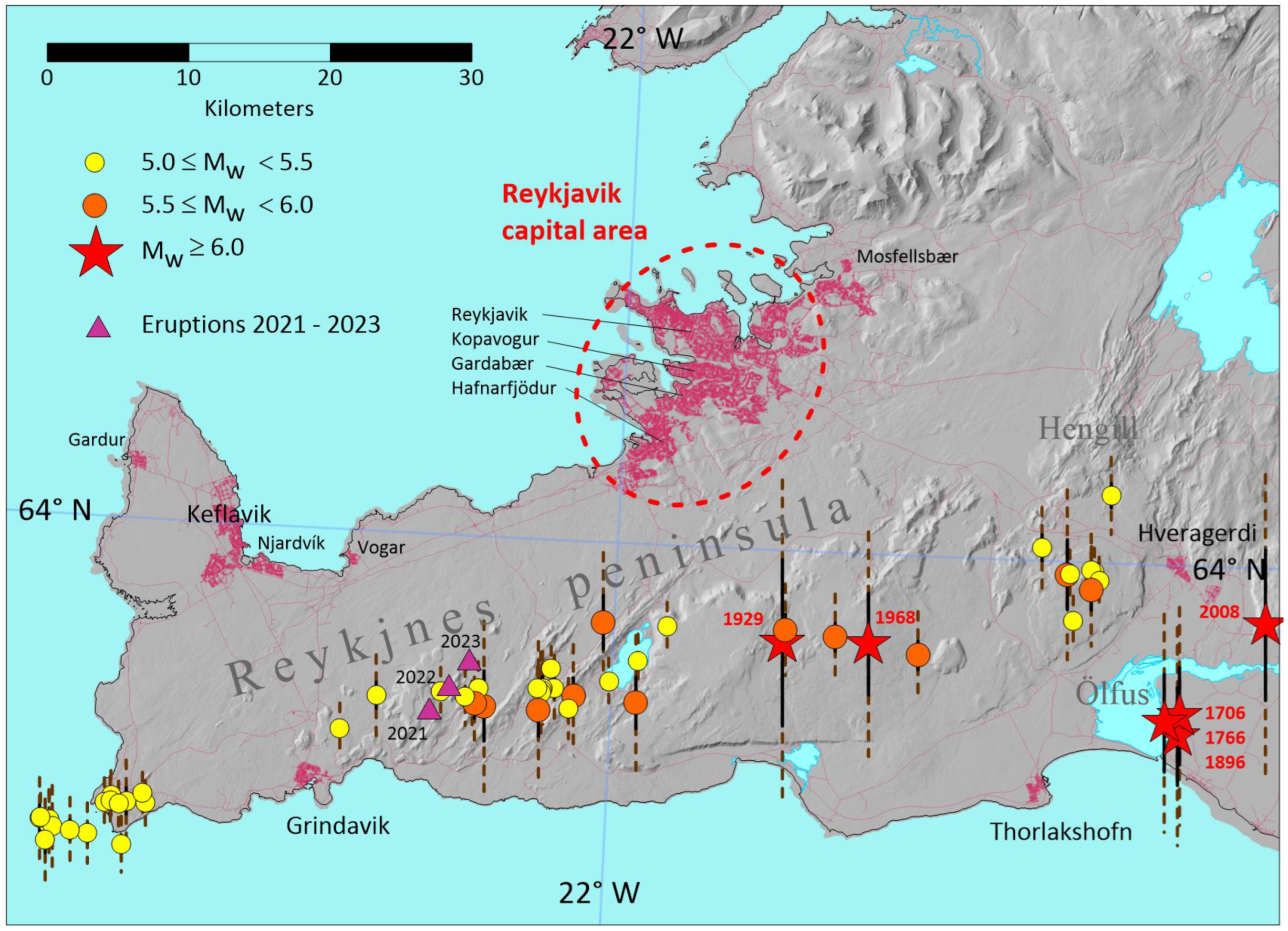
2.1. Seismic Hazards in the Reykjanes Peninsula

About two-thirds of the population of Iceland lives in the Reykjavik capital area (RCA). The capital area is in the north-east part of the Reykjanes Peninsula, which is an active seismic and volcanic zone (Figure 2) [22]. In a new harmonised earthquake catalogue for Iceland covering the instrumental period from 1900–2019, a total of 53 earthquakes of magnitude $M_w\ge 5.0$ are reported in the Reykjanes Peninsula and Ölfus, the western part of the South Iceland Seismic Zone (SISZ) (Figure 2) [12]. Of these, three earthquakes had a magnitude greater than six: $M_w$6.36 in 1929, 6.12 in 1968, and 6.31 in 2008. The first two had an epicentral distance of less than 20 km from the outskirts of the RCA. In addition, three historical earthquakes in the period 1700–1900, all with an estimated $M_{w}6.1,$struck in Ölfus in 1706, 1766, and 1896, respectively (Figure 2) [12].

The main characteristic of the seismicity on both the Reykjanes Peninsula as well as in the SISZ are shallow (5–10 km), strike-slip earthquakes with N–S faulting and vertical fault planes (dip angle ~90°) [23]. The estimated upper magnitude bound for earthquakes in the Reykjanes Peninsula is $M_{w}6.5$. This is supported by historical and instrumentally recorded earthquakes as well as geological evidence. Further east, in the SISZ, bigger events are known to occur [12]. In that area, the crust is thicker and capable of storing larger seismic strains. The fault lengths shown in Figure 2 are based on models by Wells and Coppersmith [24], and the epicentre is placed in the middle of the fault.

Figure 2. Reykjanes peninsula. Red thin lines show the road system and thicker red lines can be used to identify settlements and towns. Instrumental recorded earthquakes in the period from 1900–2019 with $M_w\ge 5.0$ and three historical earthquakes from 1700 to 1900 with $M_w\ge 6.0$ in the Ölfus region are shown [12]. The largest events (red stars) are marked with the year they struck. The black lines indicate computed surface fault rupture and the dotted brown lines the subsurface rupture based on the rupture model by [24]. Eruptions in the period 2021 to 2023 are marked with violet triangles and year.

Figure 2. Reykjanes peninsula. Red thin lines show the road system and thicker red lines can be used to identify settlements and towns. Instrumental recorded earthquakes in the period from 1900–2019 with $M_w\ge 5.0$ and three historical earthquakes from 1700 to 1900 with $M_w\ge 6.0$ in the Ölfus region are shown [12]. The largest events (red stars) are marked with the year they struck. The black lines indicate computed surface fault rupture and the dotted brown lines the subsurface rupture based on the rupture model by [24]. Eruptions in the period 2021 to 2023 are marked with violet triangles and year.

Late in the year 2020, the seismic activity greatly increased in the western part of the Reykjanes Peninsula due to magma intrusion and volcanic activity, which has so far resulted in three eruptions. The first eruption started on 19 March 2021 and lasted for a few months. The second eruption, which began on 3 August 2022, was relatively brief, lasting only two weeks. The third eruption initiated on 10 July 2023 and endured for few weeks (Figure 2). Intense seismicity preceded all these eruptions. In the period from October 2020 to October 2023, six earthquakes of $M_w\ge 5.0$ occurred in the area close to the eruptions. The largest event was $M_w=5.6$ on 24 February 2021 [25]. Historical and geological information indicate that the incipient volcanic and associated seismic activity in the region might last for many decades to come [26]. The seismicity in the period prior to the eruptions caused discomfort among the residents in the small towns closest to eruption, mainly in Grindavik, which was the closest, but also in Vogar and Njardvik. The ground shaking was also clearly felt in the RCA. Nevertheless, these events only caused minor damage related to cosmetic and non-structural losses (objects falling on flooring, etc.). In total, 25 insurance claim payouts were made by Natural Catastrophe Insurance of Iceland [27], which is a public institution that oversees the insurance of buildings and other properties in Iceland against natural disasters like earthquakes. In Iceland, all real estate is mandated by law to be insured against natural disasters. At present, the deductible is EUR ~2600 for each property for a given damaging event. This means that although the losses in the above 25 cases were minor, they were nevertheless higher than the deductible. The ongoing activity in the area has the potential to trigger larger tectonic earthquakes in a magnitude range like those in 1929 and 1968 (see Figure 2).

2.2. Exposure Data

The building stock in the Reykjavik capital area (Reykjavík, Kópavogur, Gardabær, Hafnafjördur and Seltjarnarnes) has quite a different composition than the building mass in the SISZ contained in the two datasets (see Section 3.2). In Figure 3, the dwellings in RCA are classified according to the building material, number of storeys, and code level. Around 95% of the dwellings are in buildings made of concrete or concrete+other material, whilst only 1% of the dwellings are in masonry buildings. Around 26% of dwellings are in 1–2-storey buildings and 56% are in 3–5-storey buildings. Finally, 62% of the dwellings are buildings designed in the moderate-code and high-code period (see

Table 1. Status of seismic design codes in Iceland for different construction periods.

Status	Description	Comment	Period
CDN	No-code	No seismic design code	<1958
CDL	Low-code	First generation of seismic codes	1958–1975
CDM	Moderate-code	Second generation of seismic codes	1976–2001
CDH	High-code	Latest generation of seismic codes	≥2002

). The lateral load resisting system for most of the building stock is structural walls like in the SISZ. The RCA has expanded in recent decades. Therefore, most of the moderate-code and high-code buildings are in the suburbs of the municipalities closest to the fault rupture of the scenario event of 1929 (Figure 2). Apartment buildings are common in the new districts and all the storey classes in Figure 3b can on the other hand be found almost everywhere within the RCA.

3. Loss Data and Empirical Vulnerability Model

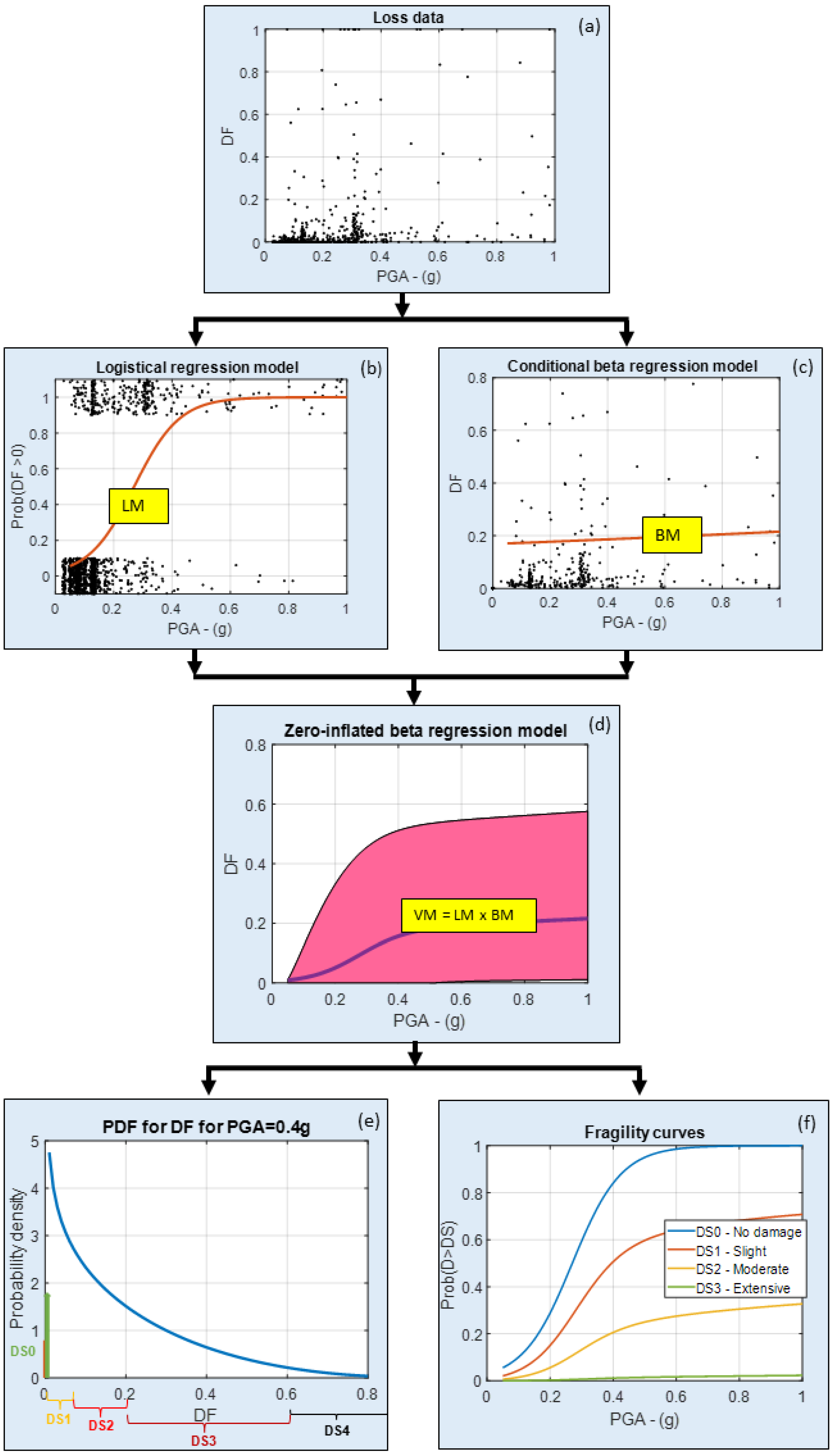
3.1. Loss Data

It is mandated by law in Iceland to have insurance against destructive natural events. This includes events like earthquakes, landslides, avalanches, floods, etc. The insurance is a part of the fire insurance terms. If a property has fire insurance, it also has natural disaster insurance. The insurance is managed by Natural Catastrophe Insurance of Iceland (NCI) [27]. After the June 2000 earthquakes, the repair cost of damaged properties was estimated by trained assessors to fulfil insurance claims. The affected area is an agricultural region with farms, settlements, small towns, and all the infrastructure assets of a modern society. The two events in June 2000 occurred within only four days, and therefore the observed damage may include accumulate damage from both events. The distance between the fault ruptures of the 17 June and 21 June events is approximately 16 km (Figure 1). The attenuation of wave propagation is high in Iceland due to a geologically young and cracked volcanic bedrock and layered lava fields. In [13], it was argued that almost all the damaged buildings in June 2000 were only affected by the earthquake closest to the building in question. Only very few buildings were in the middle area at a similar distance from each fault, and thereby affected “equally” by both events (Figure 1). In the 2000 dataset, each loss unit refers to a “building” where a building is defined from a street address (see [16] for more details).

After the May 2008 earthquake, similar methods as for the 2000 earthquakes were used to assess repair cost to establish the 2008 loss dataset. In the 2008 dataset, the loss unit is a “dwelling”. In 2000 and 2008, the insurance deductible was low (EUR 650 per dwelling). This low value encouraged all owners to report damage to their properties to receive insurance payback. This is the main reason for the assumption that both the 2000 and the 2008 datasets are complete and include all affected buildings in the region (PGA > 0.05 g) which is rare to find in other studies [29]. The deductible has now been raised to EUR ~2600 per dwelling.

The two datasets cover the loss estimates for both structural and non-structural elements. The term “non-structural elements” includes cladding, flooring, fixtures, and technical systems (electrical installations, plumbing, etc.). Damage to the building content, that is, loose household items like furniture, TVs, computers, etc., is not included. In this study, the presented vulnerability models are assessed for the combined losses of the structural and non-structural damage given in the datasets. A damage factor, DF, is computed for each building unit, which is defined as:

$$DF=\frac{ \mathrm{Estimated} \mathrm{repair} \mathrm{cost}}{\mathrm{Fire} \mathrm{Insureance} \mathrm{Value}}=\frac{ERC}{FIV}$$

(2)

where ERC is the combined estimated repair cost. The fire insurance value (FIV) is obtained from an official property database. The FIV is estimated as the depreciated replacement value (DRV) plus the cost of dismantling and transporting the debris. The dismantling and transport cost is taken as 12% of the DRV. The DRV is based on age, construction material, and general condition. The FIV is used by NCI to define the maximum payback that a building owner can receive for a dwelling/building with “total damage” or total “loss” (DF = 1). In practice, damage equivalent to “total loss” was assigned to most of the buildings that suffered an estimated repair cost of more than 70% of their FIV value in the 2000 dataset. In the 2008 dataset, total loss was estimated on a case-by-case basis for dwellings with an estimated loss in the range 50–70% of their FIV.

3.2. Building Taxonomy of the Loss Data

The Property Registry in Iceland [28] maintains a detailed property database for all building units in Iceland. It contains information on the construction material, year of construction, number of storeys, usage (residential, service, industry, etc.), floor area, street address, GPS coordinates, fire insurance value, etc. It does not include information on the lateral load resting system or main structural system, nor about the site conditions (bedrock, soil, etc.). In this study, the GEM taxonomy was used to classify all the building units in the datasets [30]. Only residential buildings were considered. The 2000 dataset is a building-by-building set, while in the 2008 dataset is a dwelling-by-dwelling set. Most of the buildings in the datasets are one or two storeys, and in such cases, building units and dwelling units are the same.

In the 2000 dataset, 54% of the residential buildings were built of concrete (C), almost all cast-in-place (CIP); 37% were timber buildings (W) made of light wood (WLI); 9.3% unreinforced masonry buildings (MUR + CBH + MOC) built before 1976 when seismic codes were first implemented in Iceland; and the rest, 0.3%, used other construction material. Only 23 buildings, mostly made of timber, were built before 1900 and the oldest building was built in 1875. Regarding height, 68% of the buildings were one-storey, 23% two-storey, 7.9% three-storey, and 0.3% four-storey. No buildings were higher. In the 2008 dataset, where all losses refer to dwellings, 45% of them were in buildings built of concrete, 48% in timber buildings, and 7.6% in masonry buildings. Furthermore, 74% of the dwellings were in one-storey buildings, 19% in two-storey, 5.9% in three-storey, and 0.5% in four-storey buildings. In the 2008 dataset, 19 dwellings were in buildings built before 1900, and the oldest one was constructed in 1875.

Since only a low fraction of the affected buildings are three-storey or higher in both datasets, they were excluded in the modelling and the evaluated models therefore only consider one- to two-storey buildings. These buildings were combined and the class marked with HBET:1,2 according to the [30] taxonomy.

The lateral load resisting system for almost all the buildings in the two datasets are structural walls. Based on the GEM taxonomy, LWAL is therefore used to identify the structural system. In both datasets, the masonry buildings are built of unreinforced, hollow concrete blocks using light-weight pumice as the main aggregate (high-porosity volcanic rock). The foundations and the bottom slabs in both timber and masonry buildings are usually made of reinforced concrete. Concrete frame buildings with stone or brick infills, which are common in South Europe, do not exist in Iceland. For more details of the building characteristic, see [17].

Crowley et al. [31] classified the status of seismic design codes in different European countries, including Iceland, into four categories based on the construction period (Table 1). In [17], it was concluded that no-code and the low-code (CDN + CDL) buildings could be combined into one class, and the moderate-code and the high-code (CDM + CDH) buildings into one class. However, in the 2000 dataset, no building belongs to the high-code period, which started in 2002. Only one class, CDN + CDL, is available for masonry buildings, as most of them, 98%, were built before 1976. The 2% remainder were not used in the model calibration.

Table 2. Classification of residential buildings affected by the June 2000 and May 2008 earthquakes.

Short Name	GEM Building Taxonomy	2000 Dataset		2008 Dataset
		Number	(%)	Number	(%)
C-NL	CR + CIP/LWAL/HBET:2,1/CDN + CDL	1665	35	1112	23
C-M or C-MH 1	CR + CIP/LWAL/HBET:2,1/CDM + CDH	907	19	1003	21
W-NL	W + WLI/LWAL/HBET:2,1/CDN + CDL	692	15	649	14
W-M or W-MH 1	W + WLI/LWAL/HBET:2,1/CDM + CDH	1047	22	1623	34
M-NL	MUR + CBH + MOC/LWAL/HBET:2,1/CDN + CDL	443	9.3	359	7.6
	Total sum	4754	100	4746	100

¹ C-M and W-M refer to the 2000 dataset since that dataset includes no high-code buildings, whilst C-MH and W-MH refer to the 2008 dataset.

sums up how the building units in the two loss datasets are distributed into the five building typologies used in this study.

3.3. Vulnerability Model

In the June 2000 and May 2008 earthquakes, a high proportion of the buildings/dwellings in the affected area (PGA > 0.05 g) had no losses, DF = 0, whilst buildings with total losses, DF = 1, were rare in both datasets. In between these extremes are a number of building units with some loss, that is, a DF in the range 0 to 1. Since the loss dataset includes “zero” and “one” values and then many values in between, it is preferable to use a mixed continuous–discrete regression to model the data, that is, discrete models to cover the DF = 0 and DF = 1 cases, and then continuous regression for loss data in the range (0, 1). The beta probability distribution is flexible and can take a wide range of shapes. It is also bounded in the interval (0, 1) and is therefore suitable to cover the continuous regression in the model. Beta distribution was used in ACT-13 [4,5] to model losses, where judgement-based methods were applied. In the GEM guidelines for empirical vulnerability assessment [29], beta regression is mentioned as potential future method. In this study, where the data include a high fraction of zero-loss incidents but only small number of total losses, a zero-inflated beta regression model is well suited [32]. This is an improved beta regression model to take care of zeros. The discrete modelling of the total loss buildings (DF = 1) is excluded, but instead the DF for these buildings is assigned a value less than 1. This model has been used earlier to model both the 2000 dataset and the 2008 dataset using the PGA as the intensity measure in a five-parameter model for each building typology [13,17].

A two-step regression process is used to construct the vulnerability model. This approach is explained schematically in Figure 4 using the PGA as intensity measure and the loss data from the 2000 dataset for the C-NL class (1665 datapoints, see Table 2). The PGA can be replaced with any other desired intensity measure or its proxy, like for instance, the Joyner–Boore distance, R_JB, as in Section 4. In Figure 4a, the loss data (raw data) are shown. Each point indicates the estimated DF based on Equation (2) for the given building unit and the computed PGA at the property site in question. In Figure 4b, the loss data are transformed into binomial variables, i.e., Y = 0 if DF = 0 and Y = 1 if DF > 0. The data points are jittered in the range $\left[-0.05, 0.05\right]$for Y = 0 and in the range $\left[0.95, 1.05\right]$for Y = 1 to better show the density of the data points. A logistical regression model (LM), which is a type of generalised linear model, is then used to analyse the relationship between Y and the PGA, that is, to model the probability of obtaining loss as a function of the PGA. The logistical model for each building typology is given as:

$${\log }_e\left(\frac{p}{1-p}\right)={\beta }_0+{\beta }_1\cdot PGA$$

(3)

where ${\beta }_0$ and ${\beta }_1$ are regression parameters and $p$ is the probability of sustaining losses (DF > 0) (Figure 4b). The parameters of the model are computed using the general linear model package, glm, in R [33].

A beta regression [34] is carried out for the data points with a DF > 0 to model the continuous loss distribution (Figure 4c). The beta probability density function (PDF) is given as:

$$f\left(x;\mu ,\phi \right)=\frac{\Gamma \left(\phi \right)}{\Gamma \left(\mu \phi \right)\Gamma \left(1-\mu \right)\phi }{x}^{\mu \phi -1}{\left(1-x\right)}^{\left(1-\mu \right)\phi -1}$$

(4)

where x is the random variable in the range (0, 1); $\mu$ is the mean; $\phi$ the precision; and $\Gamma (·)$ is the gamma function. The mean and precision of the beta PDF are related to the linear predictors η₁ and η₂ using link functions, g₁(·) and g₂(·). The linear predictors are a function of the ground shaking intensity measure or its proxy. The link functions must be strictly monotonic and differentiable twice. The logit link function was adopted for μ, and the log link function for φ:

$$g_1\left(\mu \right)=\mathrm{logit}\left(\mu \right)=\log \left(\frac{\mu }{1-\mu }\right)={\eta }_1$$

(5)

$$g_2\left(\phi \right)=\log \left(\phi \right)={\eta }_2$$

(6)

The first predictor is a function of the intensity measure while the second is a constant:

$${\eta }_1={\theta }_0+{\theta }_1\cdot {\log }_e\left(PGA\right)$$

(7)

$${\eta }_2={\theta }_0^{\prime }$$

(8)

where ${\theta }_0$, ${\theta }_1$, and ${\theta }_0^{\prime }$ are regression coefficients. The beta regression is carried out in R [33] using the betareg package. Finally, the logistical model and the conditioned beta model are combined to obtain the vulnerability model (Figure 4d). Hence, for a given building typology, five parameters $\left\{{\beta }_0, {\beta }_1, {\theta }_0, {\theta }_1, {\theta }_0^{\prime } \right\}$ define the vulnerability model. The expected value and the variance of the DF for the combined model are given as:

$$E\left[DF\right]=p\cdot \mu$$

(9)

$$Var\left[DF\right]=p\cdot \frac{\mu \cdot \left(1-\mu \right)}{\phi +1}+\left(1-p\right)\cdot p\cdot {\left(\mu \right)}^2$$

(10)

The total probability theorem can then be used to compute the desired prediction interval:

$$\mathrm{P}\left[X<x\right]=1+p\cdot \left(F_X(x,\mu ,\phi )-1\right)$$

(11)

where F_X(x,μ,φ) is the beta cumulative distribution function (CDF) for a given building typology, which is a function of the PGA. Hence, from the vulnerability model, it is possible to directly compute the PDF for the random variable DF for any given PGA. An example of this is shown in Figure 4e for a PGA = 0.4 g. Finally, by defining bins for different damage stages, fragility curves can be constructed using Equation (11). The loss bins and the verbal description of every damage state here are based on [35] (see

Table 3. Definitions of damage states in this study.

Damage State	Description	DF Bins
DS0	No damage	DF = 0
DS1	Slight damage	0.00 < DF ≤ 0.05
DS2	Moderate damage	0.05 < DF ≤ 0.20
DS3	Extensive damage	0.20 < DF ≤ 0.50
DS4	Complete damage	DF > 0.5

). Fragility curves based on the procedure are shown in Figure 4f. For more details, see Bessason et al. [17].

4. Results and Discussion

4.1. Vulnerability Curves and Fragility Curves

By replacing the PGA in Equations (3) and (7) with the Joyner–Boore distance, R_JB, a new set of model parameters were estimated for the ZIBR model. To account for outliers in the two datasets, as applied in previous studies [13,17], all data points with a DF > 0.85 were replaced with a max value of DF_max = 0.85. This was carried out for 15 concrete, 5 timber, and 13 masonry buildings in the 2000 dataset, and for 4 concrete, 7 timber, and 12 masonry dwellings in the 2008 dataset. Furthermore, the same type of data weighting was performed as in [13,17]. The model parameters are given in

Table 4. Estimated model parameters for the ZIBR model using the Joyner–Boore distance as intensity measure. See Table 2 for definition of building typologies.

Dataset	Building Typology	${\mathit{\beta }}_0$	${\mathit{\beta }}_1$	${\mathit{\theta }}_0$	${\mathit{\theta }}_1$	${\mathit{\theta }}_0^{\mathbf{\prime }}$
2000	C-NL	1.748	−0.202	−1.798	−0.148	1.592
2000	C-M	0.800	−0.167	−2.505	−0.155	2.648
2000	W-NL	1.147	−0.192	−1.490	−0.215	1.480
2000	W-M	1.098	−0.268	−2.765	−0.029	2.371
2000	M-NL	1.823	−0.191	0.0075	−0.616	0.964
2008	C-NL	2.551	−0.388	−2.327	−0.201	2.851
2008	C-MH	2.018	−0.386	−2.928	−0.204	3.756
2008	W-NL	0.764	−0.185	−2.389	−0.020	2.395
2008	W-MH	0.748	−0.175	−2.997	−0.160	3.635
2008	M-NL	2.094	−0.302	−1.307	−0.247	1.185

for the building typologies defined in Table 2. The vulnerability curves using R_JB as an intensity parameter are shown in Figure 5 for five building typologies for each dataset (Table 2). For the 2000 dataset, corresponding to a $M_{w}6.5$ event, the mean DF is down to 0.01 (1% loss) at a less than 20 km distance for all the four concrete and timber building classes (Figure 5a,c,e,g) and at 23 km for the masonry buildings. For the 2008 dataset, corresponding to a $M_{w}6.3$ event, the mean DF is at 0.01 at less than 15 km for all the five building typologies (Figure 5b,d,f,h,j). In Figure 6, the fragility curves computed directly from the vulnerability model using the damage state definitions given in Table 3 and Equation (11) are shown. As an example, at a 20 km fault distance (R_JB), the probability of exceeding DS1 (slight damage) is less than 5% for all the 1–2-storey concrete and timber buildings based on the model from the 2000 dataset. For the 2008 dataset, the corresponding distance is 15 km. Similarly, the probability of exceeding DS2 (moderate damage), that is, when the DF exceeds 0.20 (20% loss), is approximately zero at a Joyner–Boore distance of 20 km or more for no-code and low-code concrete buildings based on the 2000 dataset (Figure 6a). For the 2008 dataset and the same building typology, the probability of exceeding DS2 at a 10 km distance or more (Figure 6b) is approximately zero. In all cases, the probability of exceeding DS4 is very low.

An indicator of the reliability of the vulnerability models in Figure 5 can be measured by using them to simulate both the mean DF, and the accumulated loss in the 2000 and 2008 earthquake and compare the results to actual observations. The result of this simulation for each building typology and each dataset is shown in

Table 5. Ratio of simulated mean DF to actual mean DF from loss data (R_DF), and ratio of simulated accumulated loss to actual accumulated loss (R_Loss) for the five building typologies.

	Dataset	C-LN	C-M or C-MH	W-NL	W-M or W-MH	M-NL	Mean
RDF	2000	0.94	0.99	0.81	0.90	0.87	0.90
RDF	2008	1.07	0.98	1.09	0.94	1.18	1.05
RLoss	2000	1.17	1.06	1.12	1.11	1.11	1.11
RLoss	2008	1.06	0.99	1.00	1.03	1.13	1.04

. The ratios are within reasonable limits: the lowest ratio for R_DF is 0.81 and the highest is 1.18. For R_Loss, the lowest ratio is 0.98 and the highest is 1.17. This indicates that the ZIBR model calibrated for the Joyner–Boore distance provides acceptable results which are comparable to the results obtained using the PGA as an intensity measure (see [17]).

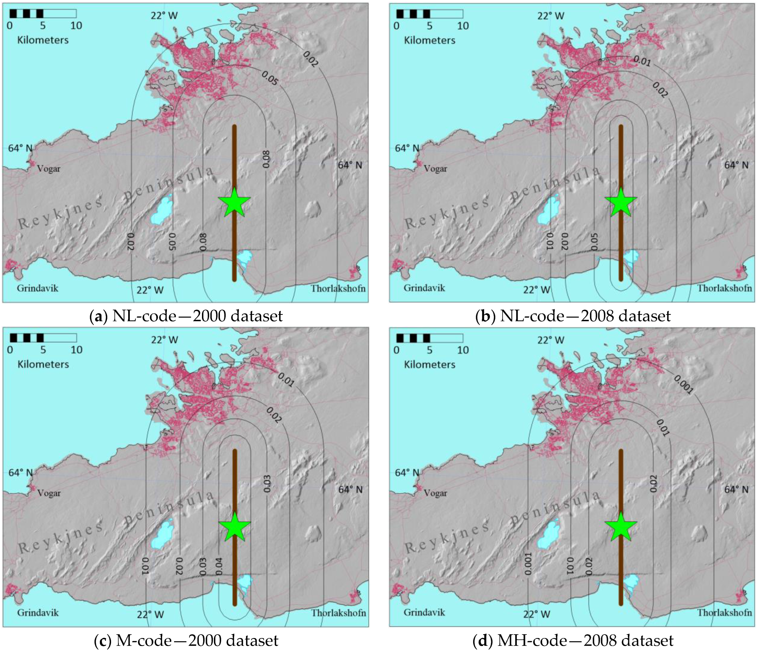
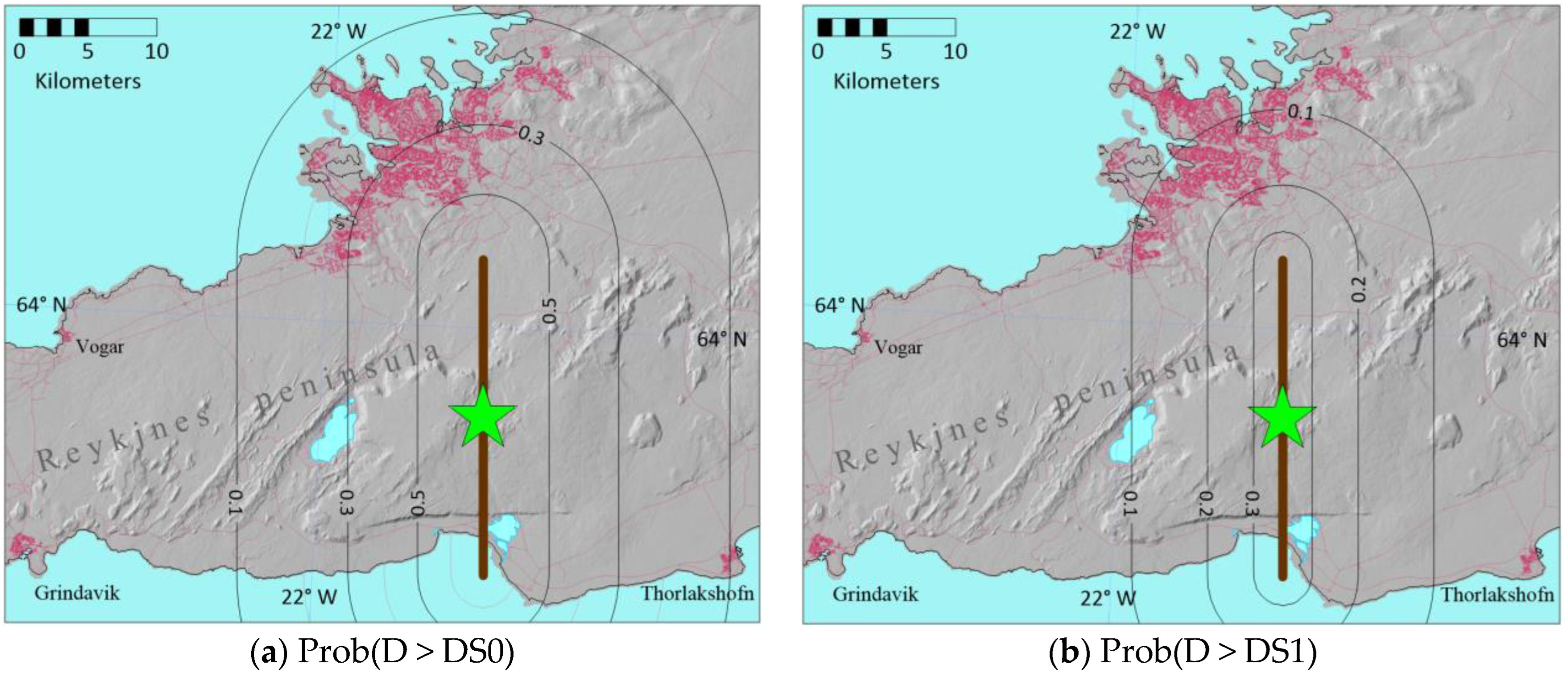
4.2. Scenario-Based Risk Maps

By using the vulnerability functions in Figure 5, scenario risk maps can be constructed. The $M_{w}6.36$ earthquake on 23 July 1929 with an epicentre 21.75° W and 63.95° N [12] is used as the scenario (see Figure 1). This event can be considered to have the most effect in the RCA of all known historical and instrumentally recorded events in the vicinity of Reykjavik. The subsurface rupture model by Wells and Coppersmith [24] is used to estimate the projected fault line on the surface (brown dotted line in Figure 1), which is then used to compute the Joyner–Boore distance. It is assumed that the epicentre lies at the centre of the fault. Since the residential building stock in the RCA mainly (>92%) consists of concrete buildings (Section 2.2), only such buildings are considered. Figure 7 shows risk maps in the form of the mean damage factor for one- to two-storey residential concrete buildings. Contours for the mean loss are shown for no-code and low-code buildings in Figure 7a using the vulnerability functions from the 2000 dataset and in Figure 7b for the vulnerability curves based on the 2008 dataset. Figure 7c shows the contours for mean damage for moderate-code concrete buildings based on the 2000 dataset and Figure 7d for moderate- and high-code buildings based on the 2008 dataset. If the dataset from 2000 is considered as representative for an $M_{w}6.5$ event and the dataset from 2008 as representative for an $M_{w}6.3$ event, it is clear how the magnitude affects the extent of the damage. The effect of the seismic code level is also clearly distinguished.

The maps in Figure 7 give useful information on the mean losses, which is important for disaster insurance purposes, but they provide no information on the distribution of the losses at different sites, which is important for emergency management. For instance, information on how many buildings (in percentage) are undamaged and how many are extensively damaged is not available in this representation. This information can be displayed by constructing scenario risk maps for damage states based on the fragility curves in Figure 6. In Figure 8, risk maps for one- to two-storey concrete residential buildings designed in the no-code and low-code period, i.e., before 1976, are shown for damage states DS0, DS1, DS2, and DS3 based on the 2000 dataset corresponding to an event of $M_{w}6.5$. As an example, Figure 8a shows the probability of exceeding DS0 (no damage). For the greatest part of the RCA, the probability of sustaining losses is 40–60%. For central Reykjavik, the probability is between 20–40%. On the other hand, the probability of exceeding DS3 and obtaining more than a 50% loss is in all cases less than 2% (Figure 8d). In Figure 9, corresponding risk maps are shown for the same building typology, except now the results are based on fragility curves calibrated from the 2008 dataset, corresponding to an event of $M_{w}6.3$. From Figure 9c, the probability of exceeding DS2 with more than a 20% loss is less than 2% in all cases.

In Figure 10, scenario risk maps are shown for one- to two-storey concrete residential buildings designed in the moderate-code period after 1976, for damage states DS0 and DS1, based on the 2000 dataset (M_w6.5). As an example, the probability of exceeding DS1 (minor damage) is close to 20% for the most exposed building sites (Figure 10b). Finally, in Figure 11, risk maps for one- to two-storey concrete residential buildings designed in the moderate-code and new-code period, i.e., after 1976, are shown for damage states DS0 and DS1, based on the 2008 dataset (M_w6.3). The probability of exceeding DS1 (minor damage) is close to 10% for the most exposed building at the outskirts of the RCA.

5. Conclusions

In this study, advanced empirical vulnerability models and fragility functions for low-rise, one- to two-storey residential buildings are presented. The building typology is defined in terms of the main building material (concrete, timber, and masonry) as well as the level of seismic codes, where no-code and low-code buildings are grouped together, and moderate-code and high-code buildings are grouped together. The vulnerability model based on zero-inflated beta regression was calibrated for two loss datasets, independently. One of the datasets is from two ~$M_{w}6.5$ strike-slip shallow earthquakes in 2000 and other one is from an $M_{w}6.3$ strike-slip shallow event in 2008. Both datasets are from South Iceland, where the earthquakes affected buildings with similar characteristics. In this study, the Joyner–Boore distance, $R_{JB}$, is used as a proxy for an intensity measure, instead of the commonly used measures like the PGA, Sa, AvgSa, etc. This approach makes the vulnerability model independent of a particular ground motion prediction model (GMPM) and is well suited for scenario-based applications where the earthquake size is fixed, and the intensity is mainly a function of the source-site distance. The application is valid for uniform site conditions, and local amplifications are not accounted for directly. However, if data allows, local effects could be incorporated by creating separate vulnerability models for different site conditions, which is not the case in this study. This representation of seismic vulnerability is simpler and more comprehensible to important stakeholders such as emergency planners, civil protection authorities, and decision-makers in risk reduction and management operations. It is also well suited for demarking spatial zones of different risk levels for a given earthquake scenario, and is therefore valuable for emergency response planning.

The presented vulnerability models show that at a distance of 10 km or more ($R_{JB}$) from the fault rupture, the mean loss is less than 5% of the replacement value for concrete and timber buildings, but higher for masonry buildings. The fragility curves show that the probability of exceeding DS2, i.e., moderate damage and exceeding losses greater than 20% of the fire insurance value, is very low (<4%) at all distances for moderate-code and high-code concrete and timber buildings. These results are valid for both $M_{w}6.3$ and $M_{w}6.5$ earthquakes.

Scenario seismic risk maps, based on the most damaging earthquake scenario in the vicinity of the RCA, that is the July 1929 $M_{w}6.36$ earthquake, were computed for low-rise concrete buildings, showing both the predicted mean loss and probability of exceeding different damage states. Although there is a lot of uncertainty about fault lengths, magnitude size, exact epicentre, as well as wave propagation and attention, the maps give a useful indication of what damage can be expected for earthquakes in the range 6.3 to 6.5 for one- to two-storey buildings. The study shows that there is considerable difference in the expected damages for 6.3 and 6.5 events. Furthermore, the code levels used in the design are easily visible on the maps. Here, it should be kept in mind that the newer buildings, which are moderate-code or high-code buildings, are generally located in the outskirts of the RCA (Reykjavik, Kopavogur, Gardabær, and Hafnafjördur), and therefore closest to the active seismic zones on the Reykjanes Peninsula.

The two complete datasets from the 2000 and the 2008 South Iceland earthquakes mainly contain one- to two-storey residential buildings (>90%) and therefore the available local empirical vulnerability models only cover these types of buildings. Nearly 60% of dwellings in the RCA are in three- to five-storey concrete apartment buildings, where the lateral load resisting system is structural walls. It is therefore a great challenge and a subject for further research to develop reliable vulnerability models for such buildings. An analytical approach based on non-linear numerical modelling of structures is a viable alternative for such research.

References

1. Bruneau, M.; Reinhorn, A. Exploring the concept of seismic resilience for acute care facilities. Earthq. Spectra 2007, 23, 41–62. [Google Scholar] [CrossRef]
2. Sangaki, A.H.; Rofooei, F.R.; Vafai, H. Probabilistic integrated framework and models compatible with the reliability methods for seismic resilience assessment of structures. Structures 2021, 34, 4086–4099. [Google Scholar] [CrossRef]
3. Forcellini, D. An expeditious framework for assessing the seismic resilience (SR) of structural configurations. Structures 2023, 56, 105015. [Google Scholar] [CrossRef]
4. ATC-13; Earthquake Damage Evaluation Data for California. Applied Technology Council: Redwood City, CA, USA, 1985; pp. 1–492.
5. ATC-13-1; Commentary on the Use of ATC-13 Earthquake Damage Evaluation Data for Probable Maximum Loss Studies of California Buildings. Applied Technology Council: Redwood City, CA, USA, 2002; pp. 1–66.
6. Rota, M.; Penna, A.; Magenes, G. A methodology for deriving analytical fragility curves for masonry buildings based on stochastic nonlinear analyses. Eng. Struct. 2010, 32, 1312–1323. [Google Scholar] [CrossRef]
7. Ruggieri, S.; Calò, M.; Cardellicchio, A.; Uva, G. Analytical-mechanical based framework for seismic overall fragility analysis of existing RC buildings in town compartments. Bull. Earthq. Eng. 2022, 20, 8179–8216. [Google Scholar] [CrossRef]
8. Rossetto, T.; Elnashai, A. Derivation of vulnerability functions for European-type RC structures based on observational data. Eng. Struct. 2003, 25, 1241–1263. [Google Scholar] [CrossRef]
9. Rota, M.; Penna, A.; Strobbia, C.L. Processing Italian damage data to derive typological fragility curves. Soil Dyn. Earthq. Eng. 2008, 28, 933–947. [Google Scholar] [CrossRef]
10. Colombi, M.; Borzi, B.; Crowley, H.; Onida, M.; Meroni, F.; Pinho, R. Deriving vulnerability curves using Italian earthquake damage data. Bull. Earthq. Eng. 2008, 6, 485–504. [Google Scholar] [CrossRef]
11. Pedersen, R.; Jónsson, S.; Árnadóttir, T.; Sigmundsson, F.; Feigl, K.L. Fault slip distribution of two June 2000 MW6. 5 earthquakes in South Iceland estimated from joint inversion of InSAR and GPS measurements. Earth Planet. Sci. Lett. 2003, 213, 487–502. [Google Scholar] [CrossRef]
12. Jónasson, K.; Bessason, B.; Helgadóttir, Á.; Einarsson, P.; Gudmundsson, G.B.; Brandsdóttir, B.; Vogfjörd, K.S.; Jónsdóttir, K. A harmonised instrumental earthquake catalogue for Iceland and the northern Mid-Atlantic Ridge. Nat. Hazards Earth Syst. Sci. 2021, 21, 2197–2214. [Google Scholar] [CrossRef]
13. Bessason, B.; Bjarnason, J.Ö.; Rupakhety, R. Statistical modelling of seismic vulnerability of RC, timber and masonry buildings from complete empirical loss data. Eng. Struct. 2020, 209, 109969. [Google Scholar] [CrossRef]
14. Sigbjörnsson, R.; Snæbjörnsson, J.T.; Higgins, S.M.; Halldórsson, B.; Ólafsson, S. A note on the Mw6.3 earthquake in Iceland on 29 May 2008 at 15:45 UTC. Bull. Earthq. Eng. 2009, 7, 113–126. [Google Scholar] [CrossRef]
15. Halldórsson, B.; Sigbjörnsson, R. The Mw6.3 Ölfus earthquake at 15:45 UTC on 29 May 2008 in South Iceland: ICEARRAY strong-motion recordings. Soil Dyn. Earthq. Eng. 2009, 29, 1073–1083. [Google Scholar] [CrossRef]
16. Ioannou, I.; Bessason, B.; Kosmidis, I.; Bjarnason, J.Ö.; Rossetto, T. Empirical seismic vulnerability assessment of Icelandic buildings affected by the 2000 sequence of earthquakes. Bull. Earthq. Eng. 2018, 16, 5875–5903. [Google Scholar] [CrossRef]
17. Bessason, B.; Bjarnason, J.Ö.; Rupakhety, R. Comparison and modelling of building losses in South Iceland caused by different size earthquakes. J. Build. Eng. 2022, 46, 103806. [Google Scholar] [CrossRef]
18. Rupakhety, R.; Sigbjörnsson, R. Ground-motion prediction equations (GMPEs) for inelastic response and structural behaviour factors. Bull. Earthq. Eng. 2009, 7, 637–659. [Google Scholar] [CrossRef]
19. Joyner, W.B.; Boore, D.M. Peak horizontal acceleration and velocity from strong-motion records including records from the 1979 Imperial Valley, California, earthquake. Bull. Seismol. Soc. Am. 1981, 71, 2011–2038. [Google Scholar] [CrossRef]
20. Icelandic Institute of Natural History. 2023. Available online: https://jardfraedikort.ni.is/ (accessed on 15 October 2023).
21. Atakan, K.; Brandsdóttir, B.; Halldorsson, P.; Fridleifsson, G.O. Site response as a function of near-surface geology in the South Iceland seismic zone. Nat. Hazards 1997, 15, 139–164. [Google Scholar] [CrossRef]
22. Einarsson, P. Plate boundaries, rifts and transforms in Iceland. Jökull 2008, 58, 35–58. [Google Scholar] [CrossRef]
23. Einarsson, P.; Hjartardóttir, Á.R.; Hreinsdóttir, S.; Imsland, P. The structure of seismogenic strike-slip faults in the eastern part of the Reykjanes Peninsula Oblique Rift, SW Iceland. J. Volcanol. Geotherm. Res. 2020, 391, 106372. [Google Scholar] [CrossRef]
24. Wells, D.L.; Coppersmith, K.J. New empirical relationships among magnitude, rupture length, rupture width, rupture area, and surface displacement. Bull. Seismol. Soc. Am. 1994, 84, 974–1002. [Google Scholar] [CrossRef]
25. Hernández-Aguirre, V.M.; Rupakhety, R.; Ólafsson, S.; Bessason, B.; Erlingsson, S.; Paolucci, R.; Smerzini, C. Strong ground motion from the seismic swarms preceding the 2021 and 2022 volcanic eruptions at Fagradalsfjall, Iceland. Bull. Earthq. Eng. 2023, 21, 4707–4730. [Google Scholar] [CrossRef]
26. Sæmundsson, K.; Sigurgeirsson, M.Á. Reykjanes peninsula. In Natural Hazard in Iceland, Volcanic Eruptions and Earthquakes; Sólnes, J., Sigmundsson, F., Bessason, B., Eds.; University of Iceland Press: Reykjavik, Iceland; Natural Catastrophe Insurance of Iceland: Kópavogur, Iceland, 2013; pp. 379–401. (In Icelandic) [Google Scholar]
27. Natural Catastrophe Insurance of Iceland. 2023. Available online: https://island.is/en/o/nti (accessed on 15 October 2023).
28. Property Register. 2023. Available online: https://www.fasteignaskra.is/english (accessed on 15 October 2023).
29. Rossetto, T.; Ioannou, I.; Grant, D.N.; Maqsood, T. Guidelines for the Empirical Vulnerability Assessment; GEM Foundation: Pavia, Italy, 2014. [Google Scholar]
30. Brzev, S.; Scawthorn, C.; Charleson, A.W.; Allen, L.; Greene, M.; Jaiswal, K.; Silva, V. GEM Building Taxonomy; Version 2.0; GEM Technical Report No. 2013-02; GEM Foundation: Pavia, Italy, 2013. [Google Scholar]
31. Crowley, H.; Despotaki, V.; Silva, V.; Dabbeek, J.; Romão, X.; Pereira, N.; Castro, J.M.; Daniell, J.; Veliu, E.; Bilgin, H.; et al. Model of seismic design lateral force levels for the existing reinforced concrete European building stock. Bull. Earthq. Eng. 2021, 19, 2839–2865. [Google Scholar] [CrossRef]
32. Ospina, R.; Ferrari, S.L.P. A general class of zero-or-one inflated beta regression models. Comput. Stat. Data Anal. 2012, 56, 1609–1623. [Google Scholar] [CrossRef]
33. R Core Team. R: A Language and Environment for Statistical Computing; R Foundation for Statistical Computing: Vienna, Austria, 2023; Available online: https://www.R-project.org/ (accessed on 15 October 2023).
34. Ferrari, S.L.P.; Cribari-Neto, F. Beta Regression for Modelling Rates and Proportions. J. Appl. Stat. 2004, 31, 799–815. [Google Scholar] [CrossRef]
35. Dolce, M.; Kappos, A.; Masi, A.; Penelis, G.; Vona, M. Vulnerability assessment and earthquake damage scenarios of the building stock of Potenza (Southern Italy) using Italian and Greek methodologies. Eng. Struct. 2006, 28, 357–371. [Google Scholar] [CrossRef]
Figure 1. South Iceland Seismic Zone (SISZ). The map shows the epicentre and fault rupture of the two South Iceland earthquakes of 17 June 2000 ( M w = 6.52 ) and 21 June 2000 ( M w = 6.44 ) , and the Ölfus earthquake of 29 May 2008 ( M w = 6.31 ) .
Buildings 13 02919 g001
Figure 3. Classification of dwellings in the Reykjavik capital area, according to; (a) building material, (b) number of storeys, and (c) code level. The data behind “material” and “number of storeys” are from the official property database in Iceland accessed in August 2023 [28].
Buildings 13 02919 g003
Figure 4. Flowchart that explains the main steps in the zero-inflated beta regression model: (a) loss data form the 2000 dataset for C-NL (black dots); (b) logistical regression model (LM); (c) conditional beta regression model (BM); (d) vulnerability model (VM) obtained by combining the LM and BM; (e) probability density function for the DF for PGA = 0.4 g; (f) fragility functions based on predefined DF bins (see Table 3).
Buildings 13 02919 g004
Figure 5. Raw data (black dots) and fitted vulnerability functions for 1–2-storey buildings/dwellings based on the ZIBR model with the Joyner–Boore distance as intensity measure for no- and low-code concrete buildings/dwellings in (a) the 2000 dataset and (b) the 2008 dataset; (c) moderate-code concrete buildings in the 2000 dataset; (d) moderate- and high-code concrete dwellings in the 2008 dataset; no- and low-code timber buildings/dwellings in (e) the 2000 dataset and (f) the 2008 dataset; (g) moderate-code timber buildings in the 2000 dataset; (h) moderate- and high-code timber dwellings in the 2008 dataset; and no- and low-code masonry buildings/dwellings in the (i) 2000 dataset and (j) in the 2008 dataset.
Buildings 13 02919 g005
Figure 6. Fragility functions for one- to two-storey buildings/dwellings based on the ZIBR model with the Joyner–Boore distance as intensity measure for no- and low-code concrete buildings/dwellings (a) in the 2000 dataset and (b) in the 2008 dataset; (c) moderate-code concrete buildings in the 2000 dataset; (d) moderate- and high-code concrete dwellings in the 2008 dataset; no- and low-code timber buildings/dwellings in (e) the 2000 dataset and (f) the 2008 dataset; (g) moderate-code timber buildings in the 2000 dataset; (h) moderate- and high-code timber dwellings in the 2008 dataset; and no- and low-code masonry buildings/dwellings in the (i) 2000 dataset and (j) in the 2008 dataset.
Buildings 13 02919 g006
Figure 7. Scenario risk map showing predicted mean damage factor for one- to two-storey concrete buildings based on the vulnerability functions in Figure 5: (a) no- and low-code buildings based on the 2000 dataset ( M w 6.5 ); (b) no- and low-code buildings based on the 2008 dataset ( M w 6.3 ); (c) moderate-code buildings based on the 2000 dataset ( M w 6.5 ); and (d) moderate- and high-code buildings based on the 2008 dataset ( M w 6.3 ).
Buildings 13 02919 g007
Figure 8. Scenario risk map for one- to two-storey, no-code and low-code, reinforced concrete buildings, C-NL (built before 1976) based on a vulnerability model from the 2000 dataset ( M w 6.5 ). The maps show the probability that the damage state will (a) exceed DS0; (b) exceed DS1; (c) exceed DS2; and (d) exceed DS3.
Buildings 13 02919 g008
Figure 9. Scenario risk map for one- to two-storey, no-code and low-code, reinforced concrete buildings, C-NL (built before 1976) based on the vulnerability model from the 2008 dataset ( M w 6.3 ). The maps show the probability that the damage state will (a) exceed DS0; (b) exceed DS1; (c) exceed DS2; and (d) exceed DS3.
Buildings 13 02919 g009
Figure 10. Scenario risk map for one- to two-storey, moderate-code, reinforced concrete buildings, C-M (built after 1976) based on the vulnerability model from the 2000 dataset ( M w 6.5 ). The maps show the probability that the damage state will (a) exceed DS0 and (b) exceed DS1.
Buildings 13 02919 g010
Figure 11. Scenario risk map for one- to two-storey, moderate-code and high-code, reinforced concrete buildings, C-MH (built after 1976) based on the vulnerability model from the 2008 dataset ( M w 6.3 ). The maps show the probability that the damage state will (a) exceed DS0 and (b) exceed DS1.
Buildings 13 02919 g011