Article

Point Cloud-Based Smart Building Acceptance System for Surface Quality Evaluation

1
Seventh Engineering Bureau, CCCC Frist Highway Engineering Group Co., Ltd., Zhengzhou 451450, China
2
Department of Civil Engineering, Chongqing Jiaotong University, Chongqing 400074, China
3
Huasheng Testing Technology Co., Ltd., Chongqing 400700, China
4
Department of Civil Engineering, KU Leuven, 8000 Bruges, Belgium
*
Authors to whom correspondence should be addressed.
Buildings 2023, 13(11), 2893; https://doi.org/10.3390/buildings13112893
Submission received: 30 September 2023 / Revised: 12 November 2023 / Accepted: 17 November 2023 / Published: 19 November 2023
(This article belongs to the Special Issue New Trends on Non-destructive Testing in Construction)

Abstract

:
The current expansion of building structures has created a demand for efficient and smart surface quality evaluation at the acceptance phase. However, the conventional approach mainly relies on manual work, which is labor-intensive, time-consuming, and unrepeatable. This study presents a systematic and practical solution for surface quality evaluation of indoor building elements during the acceptance phase using point cloud. The practical indoor scanning parameters determination procedure was proposed by analyzing the project requirements, room environment, and apparatus. An improved DBSCAN algorithm was developed by introducing a plane validation and coplanar checking to facilitate the surface segmentation from the point cloud. And a revised Least Median of Square-based algorithm was proposed to identify the best-fit plane. Afterwards, the flatness, verticality, and squareness were evaluated and depicted using a color-coded map based on the segmented point cloud. The experiment on an apartment showcases how the system improves the information flow and accuracy during building acceptance, resulting in a potentially smart acceptance activity.

1. Introduction

Building structures, including office buildings, shopping malls, residential apartments, etc., have witnessed a substantial explosion in the past few decades [1]. In order to provide a safe, comfortable indoor space for human activities, the surface quality of concrete elements should be ensured prior to the acceptance in case of unexpected system failure or construction delay, which could result in increased cost. Previous studies have demonstrated that around 5% of the construction cost is caused by rework because of defects [2] and that 4% of the total value of a residential construction contract is the defects cost [3]. Therefore, a systematic and deep surface quality evaluation (SQE) of the components is quite important to reduce the cost and reduce the time to completion.
Verticality, flatness, and squareness are three important indicators [4] to evaluate the quality and aesthetic of concrete surfaces, which are widely used in practice. To elaborate, the verticality of building components indicates the deviation between the elements’ actual centroid line and the reference plane [1], which is usually quantified by the angle tolerance between them. It represents the continuity and consistency in the vertical direction of vertical elements, especially in the process of layered construction, which has a substantial impact on the vertical load transfer and capacity. The flatness indicates the deviation of the constructed surface from the reference surface, which has a great impact on the installation quality of the components attached to it and the aesthetics. Moreover, the squareness indicates the angle of any two neighboring edges of the elements or structures, which is another important indicator in the checking list.
In general, the SQE is conducted manually using the contact measuring apparatus within the building construction, such as tape, straightedges, leaning gauge, etc. [5,6]. The verticality evaluation (VE) of building structures is mainly divided into two categories: horizontal deviation method and inclination method. As shown in Figure 1a, the horizontal deviation method measures the maximum horizontal distance, d, between the tested surface and the vertical reference surface within a fixed height range. This horizontal deviation is generally proportional to the height of the layered construction, which is typically measured by theodolite, plumb-bob, optical plummet, or arc length-based method, etc. Such methods are appropriate for measuring the verticality with a relatively narrow height range, such as indoor walls, columns, etc. The second method, the inclination method, measures the angle between the line of two measured points on the surface of the structure and the vertical plane, as shown in Figure 1b, which is applicable to a wider range of elements with higher heights, such as building façades and bridge piers, etc. Similar to VE, flatness evaluation (FE) is primarily determined by measuring the maximum elevation difference between the tested surface and the reference surface within a fixed testing area as shown in Figure 1c. The 2 m leaning gauge is frequently employed, which is normally for low-height vertical components such as interior walls, beams, etc., and for horizontal elements like floors and ceilings.
Figure 2a,b indicate the widely used verticality and flatness evaluation methods with 2 m rulers and feeler gauges according to the standard [6] which are used by building developers for quality control of buildings [7]. The entire process requires two skilled technicians to sample, measure, and record, which has a low efficiency and the results are not repeatable. Furthermore, the VE requires a laser level to make sure that the 2 m ruler is in the vertical direction. For the squareness evaluation (SE), the purpose is to ensure that the two adjacent walls of the house are perpendicular to each other. As shown in Figure 2c, the Laser-liner is used to mark two reference lines La, Lb perpendicular to each other, with one of them (La) parallel to the shorter wall of the testing room. Then the distance between Lb from the longer wall is measured as di, and the range, R, is calculated as the squareness as Equation (1) says. The general tolerance of the above three indicators from different codes are summarized in Table 1.
R = max d i min d i , i = 1 , 2 , 3 , 4
The manual evaluation methods clearly indicate their shortcomings: they are labor intensive, time-consuming, and unrepeatable [7]. The above-mentioned approaches need manual instrument setup and calibration, which calls for a high level of patience and professionalism from the inspectors. In addition, the evaluation results rely on the sampling method, which is not clearly defined in the codes [6,8], and thus cannot reflect the overall quality of the concrete element. Moreover, these methodologies do not produce visual findings that are easily interpretable by both professionals and non-specialists [4]. Therefore, there is an increasing demand for a clear, effective, precise, and visual way to automatically evaluate the surface quality of concrete elements.
Due to the high accuracy (millimeter level in the effective scanning range) and scanning speed (up to 976,00 points/s), 3D laser scanning has been incredibly popular in construction and civil engineering quality assessment in recent years. For instance, Zhao et al. [11] proposed an automated procedure to recognize and measure the dimensions of rebars, concrete surface, and sleeves of PC components based on point cloud (PCD), which has improved the automation of the quality inspection process. Wang et al. [12] developed a geometry evaluation method focusing on the transverse side of the irregular precast elements’ surface using laser scanning. Celestino et al. [13] designed a close-range and low-cost dimension measurement system with a laser scanner, which was used for building façade measuring. Moreover, laser scanning is also used for the damage recognition and assessment of concrete and steel structures. For instance, Alireza et al. [14] proposed a method for evaluating the building-level damage after tornadoes using UAV-based PCD, while Zhou et al. [15] proposed the feasibility of using PCD from image-based three-dimensional (3D) reconstruction to assess the surface damage on residential buildings. As reviewed by Wang et al. [16], PCD data have been widely utilized during different phases in the construction industry, including the 3D model reconstruction, geometry quality inspection, progress monitoring, and deconstruction and waste management. These studies demonstrated that PCD has distinct advantages in the quality inspection of structures, due to its high precision, large sampling points, and visual graphical interface. Regarding the SQE, however, only a few studies [1,4,17,18] have been performed, which have focused on the prefabricated elements with small dimensions (≤20 m) or the internal walls of residence building; there is still a lack of a comprehensive and reliable automated SQE system using PCD at the building acceptance stage.
In order to overcome the limitations of manual measurement and develop the existing building acceptance approaches, this study proposes a completely automated acceptance system for assessing the flatness, verticality, and squareness of concrete elements using PCD data. The proposed system mainly includes three parts: data preparation, surface segmentation and plane fitting, and surface quality evaluation. Firstly, the efficiency and accuracy of PCD acquisition using a laser scanner are analyzed to obtain the optimal parameters for indoor PCD collection. Secondly, the surface of the as-built components is extracted from the raw PCD and the plane is fitted using the developed algorithms. Finally, the surface quality is evaluated based on the outcomes from the previous step, and the results are visualized using a color-coded map.
The rest of this paper is organized as follows: Section 2 presents the related existing works within the topic of SQE, PCD segmentation, and plane fitting. Section 3 illustrates the details of the proposed system for SQE. Subsequently, an experiment is conducted to verify the feasibility and improvement of the proposed algorithm, and a case study and the results of a real residential building are discussed in Section 4, followed by a summary and foresight of the proposed system in Section 5.

2. Related Works

2.1. SQE Using PCD

Flatness is described as the deviation that the evaluated surface has from a reference plane [19]. To improve the accuracy and efficiency, PCD-based FE is studied by several studies, which can be divided into two main categories based on the principles: the geometry-based method and the frequency-based method.
The geometry-based method is similar to manual inspection due to the principle. By comparing the measured surfaces with the reference surface, the deviation between them can reflect the flatness of the elements, which was completed in the space domain. For instance, Tan et al. [7] and Kim [1] used the BIM model as a reference to evaluate the geometric quality of precast elements. Bosche et al. [18] proposed an evaluation method by combining the PCD data with the BIM model of elements, and assessed the flatness based on the F-number method [20,21]. The key point is to register the scan with the BIM model in a uniform coordinate system, within which the principles of normal similarity and proximity [22] are widely used. Furthermore, the reference surface can also be obtained by fitting the PCD to an ideal surface according to several algorithms, such as RANSAC, the Least Squares Method (LSM), etc. For instance, Li et al. fitted the PCD data for a residential room by the RANSAC method in [4,22], and LSM in [23], respectively; both of them proved the feasibility of the proposed method. Cao et al. [24] segmented the surface PCD data by DBSCAN for the flatness evaluation of a residence room, while Shih and Wang [25] fitted the reference plane of the decoration walls and floors for finishing quality inspection by a commercial software. In addition, Nuttens et al. [26] used 3D scanning to monitor the ellipticity of a circular train tunnel based on the best-fit cylinder of the surface. However, the existing studies have only proposed implementable frameworks, with fewer in-depth studies on component/surface segmentation and plane fitting, which are the keys of SQE. As one of the keys of the evaluation result, the measurement directions and sampling methods are not clearly specified in the current standards, nor have they been discussed in detail in the existing studies. In addition, most of the previous works have not paid attention to the defects and noises on the PCD during segmentation and plane fitting, which can cause considerable errors for the reference plane generation.
On the other hand, the frequency-based method has been also proposed to rely on PCD data. Bosche et al. [27] firstly introduced the Continuous Wavelet Transform into the analysis of PCD data from the element surface, transforming the surface features in the space domain into waviness features within the frequency domain. Puri et al. [28] extended the methodology into 2D, achieving the recognition of magnitude and location of surface undulation. Neza et al. [29] applied this method to evaluate the surface waviness of different types of materials in experiments, which demonstrated the feasibility and visualization value. Nevertheless, the methodology does not establish a clear mathematical relationship between Waviness Index (WI) and surface flatness. Furthermore, the differences between various material properties can result in a different threshold of WI, which limits its wide adaptation.
Regarding the verticality of concrete elements, fewer studies have been conducted on this topic, which can be divided into two methods: the central axis method and the normal vector method. The first method connects the geometric centers of all sliced PCDs as the centerline of the component, and then calculates its deviation from the designed one. Han et al. [30] and Hamzi et al. [31] utilized this method to evaluate the verticality of bridge piers with a rectangular cross-section and a tower with a circular cross-section, respectively, and Wang et al. [32] applied it for the verticality inspection of a building façade. Within the study of Li et al. [4], the verticality of a wall was determined as the angle between the normal vector of the wall and that of the floor by fitting the planes of them, respectively, which is referred to as the normal vector method.
The squareness of structural elements is another significant item on the acceptance checklist, defined as the difference in length between the longer sides of a space (or element) [1]. Several studies have used PCD data to assess the squareness, for example, Tan et al. [7] and Kim et al. [1,33] inspected the precast elements with 3D scanning and evaluated the squareness with the above principle. According to the time and cost analysis of Terrestrial Laser Scanning (TLS)-based geometry QA/QC [34] including squareness, the TLS-based approach can reduce 60% of the time and higher cost efficiency compared with manual work when the gross floor area exceeded 666,900 m2. Meanwhile, there are several commercial software packages that enable squareness evaluation based on PCD, e.g., FARO, StructionSite, etc., but all of them are semi-automatic, which requires manual operation by choosing the suitable program and data.

2.2. Surface Segmentation and Fitting

The main geometries in the building PCDs, flat surface and curved surface [35], as well as the intersecting line between different surfaces, are valuable information for the laser scanning application. The curved surface is not discussed in this section since most of the surfaces designed in residential buildings are planar.
Since most of the buildings follow the Manhattan World scheme, i.e., a Cartesian coordinate system in which walls, floors, and ceilings are perpendicular to each other [36], the semantic segmentation of indoor PCD can be performed based on this feature, which is called the ‘prior knowledge based approach’ [16]. For instance, Cao et al. [24] and Hu et al. [37] projected the PCD onto the vertical plane (XZ plane or YZ plane) to conduct the segmentation of floors, ceilings, and walls from raw PCD, while other research [38,39,40] also sliced and projected the PCD onto the horizontal plane to isolate the walls individually, which uses the orientation feature for distinguishing elements. Similarly, the size, normal vector, point density, and the position can also be used as a basis for segmentation. Although the prior knowledge-based method is simple and efficient for simple scenarios such as indoor building, it can only work on the distinct geometric constraints defined, and most of them are semi-automatic processes.
Model fitting [41], which indicates matching the PCD to different geometries, is another widely used surface segmentation method when encountering the parametric models, such as planes, spheres, etc. Two main algorithms are widely used in previous studies, Hough Transform (HT) and RANdom SAmple Consensus (RANSAC). HT is one kind of feature extraction technique that could find out the best-fit model from PCD by detecting peaks on the parametric space of each point after voting in the transformed parametric space. For instance, several studies have applied it for line detection and plane fitting [42,43]. Furthermore, Rabbani et al. [44] adopted it to detect the cylinder, and a sphere recognition method based on 3D HT was introduced in [45]. However, the high complexity and sensitivity to noise when dealing with large datasets makes it limited in terms of the segmentation of interior building elements. RANSAC, by hypothesizing an inlier group from the sample and then verifying it through iteration, eventually finds all the most compatible hypotheses for the final result [40]. As a robust nondeterministic algorithm, RANSAC is widely used in shape detection, segmentation, and fitting, such as in building façades [41,46] and indoor scenes [47,48,49]. Nevertheless, its main shortcoming is the spurious surface; it may detect a surface that does not exist although the conditions are all satisfied [41]. This may cause mis-segmentation and mis-fitting afterwards for the surface.
As a density-based clustering method, DBSCAN is a widely-used algorithm for the clustering and segmentation of building PCD due to the independence of the shape of the clusters as well as its good identification of noise [50]. Instead of pre-defining the cluster number, DBSCAN automatically determines it based on the density of the PCD, which makes it suitable for point clouds with various data distributions and shapes. Therefore, many studies [51,52] have used it for the indoor plane, cylinder clustering, and segmentation. However, one main obstacle has limited its development in the PCD segmentation of building surfaces: for points on the intersection planes, they have the same definition based on DBSCAN, which may cause the intersection planes of PCD to be interpreted as the same cluster.
With the overview above, it is clear that the existing research has demonstrated the feasibility and potential of SQE using PCD due to its high accuracy, large representative samples, and visualization interface [16]. However, the acquisition of PCD data is still a challenging problem for indoor buildings. Furthermore, an automated and reliable process should be proposed to ensure high accuracy since the component/surface segmentation, PCD sampling, and surface fitting result in the basic data source of the measurement, which determines the accuracy of the subsequent measurement results. Finally, both visualization and quantification results should be provided to locate and quantify the regions for subsequent maintenance. This study is intended to improve the above-mentioned shortcomings.

3. System Framework

The proposed SQE system is carefully discussed in this section, including the key processes and data flow. As illustrated in the flowchart (see Figure 3), the main processes include three phases: data preparation, surface segmentation and plane fitting, and SQE, described as the following:
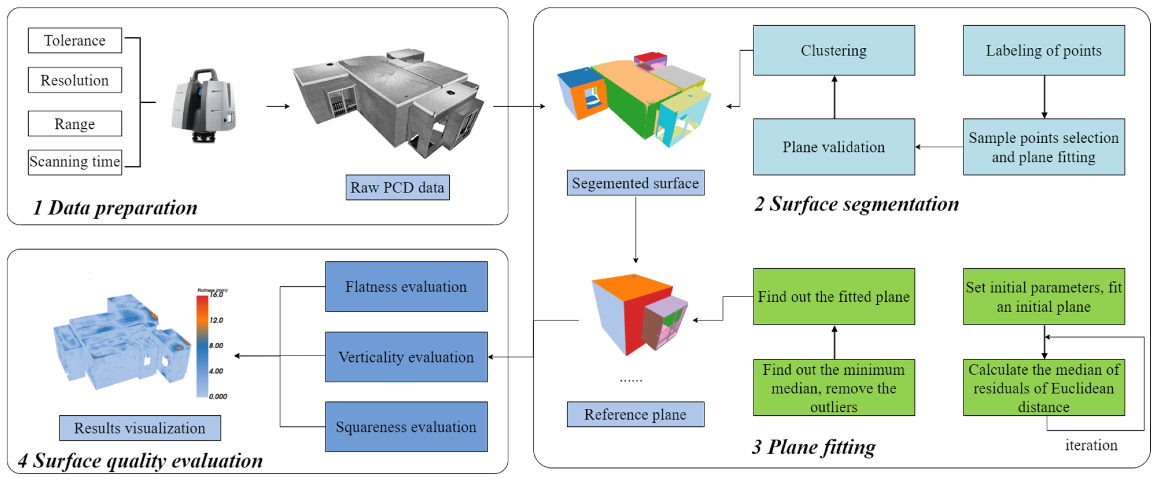
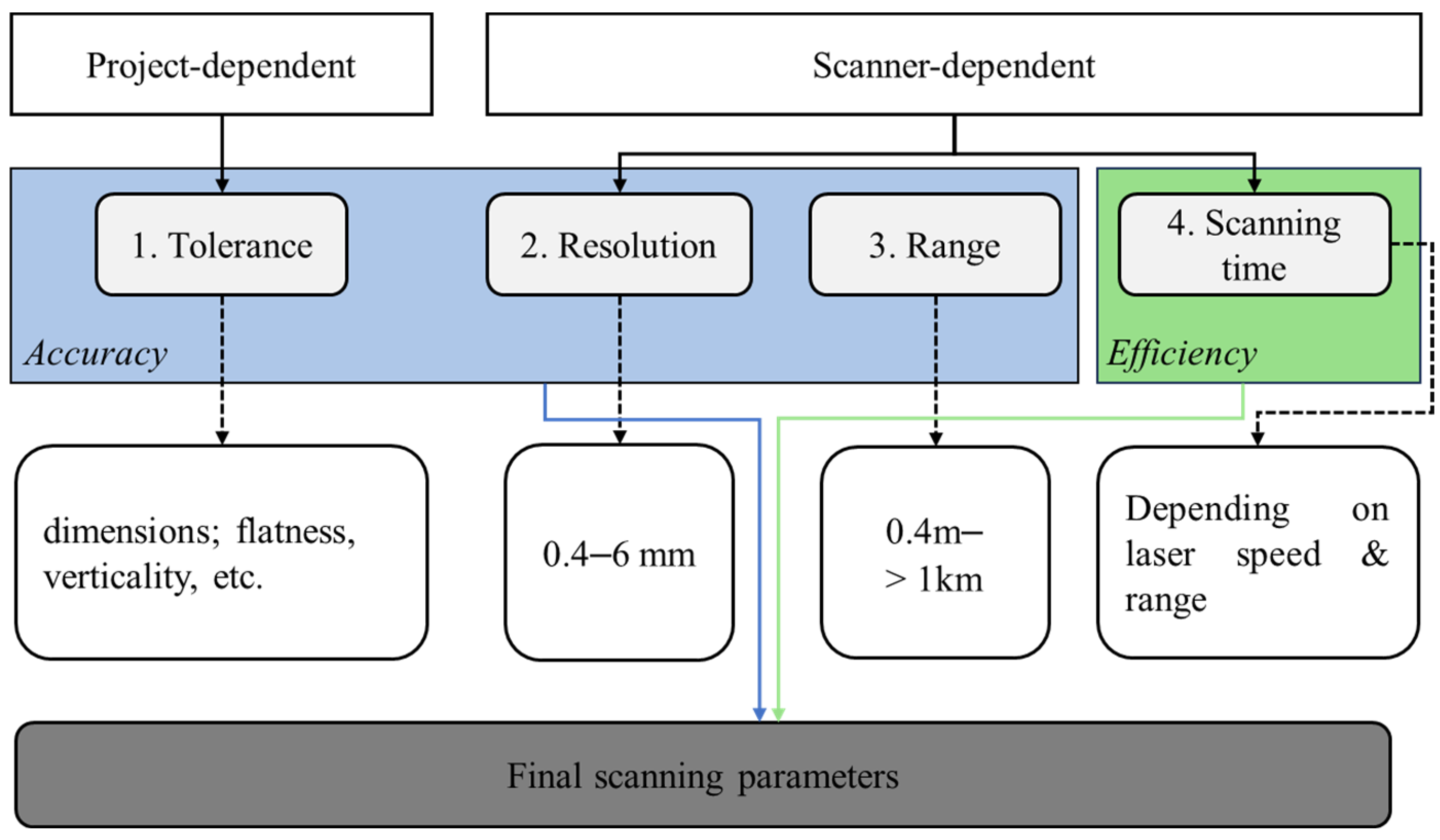
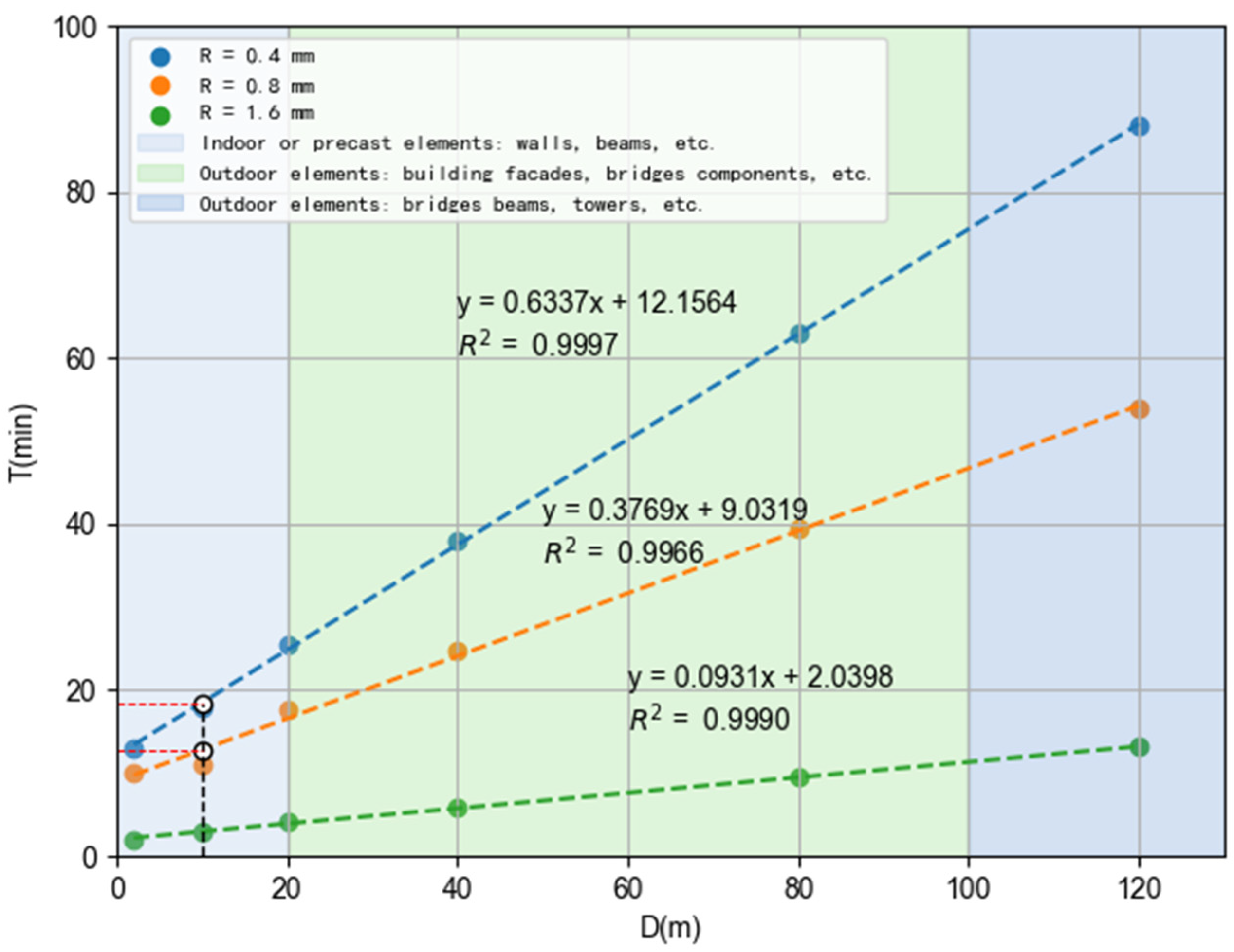
  • Data preparation. The PCD acquisition parameters and corresponding scanning modes are discussed by gathering the data from the literature and testing the scanner with different modes in the laboratory, in order to ensure the data quality. Then the dense PCD is registered and reduced for computational efficiency.
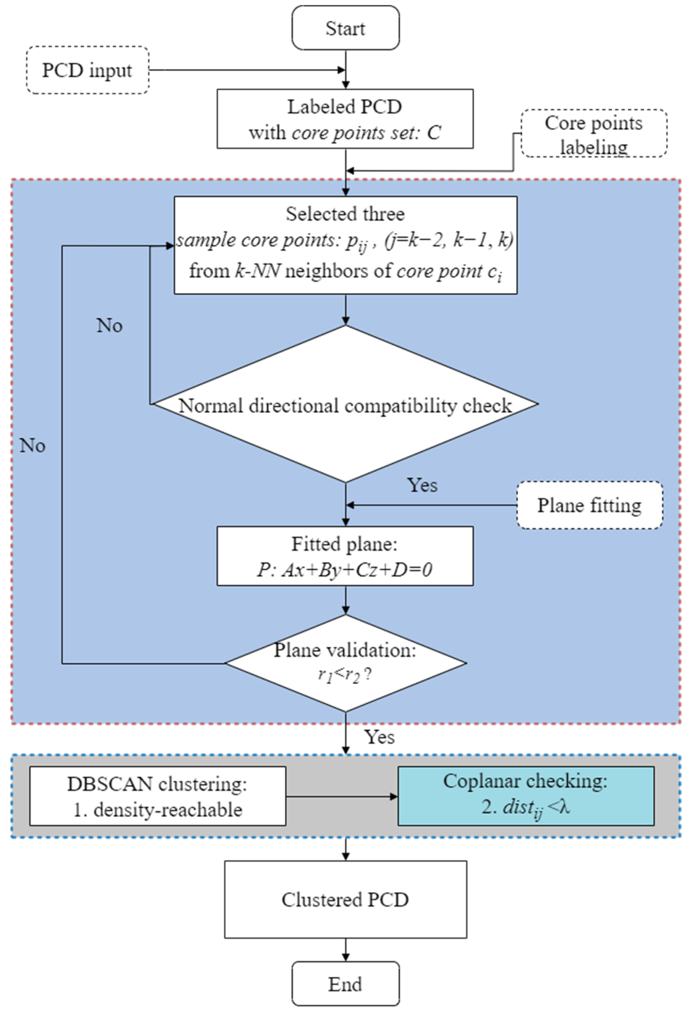
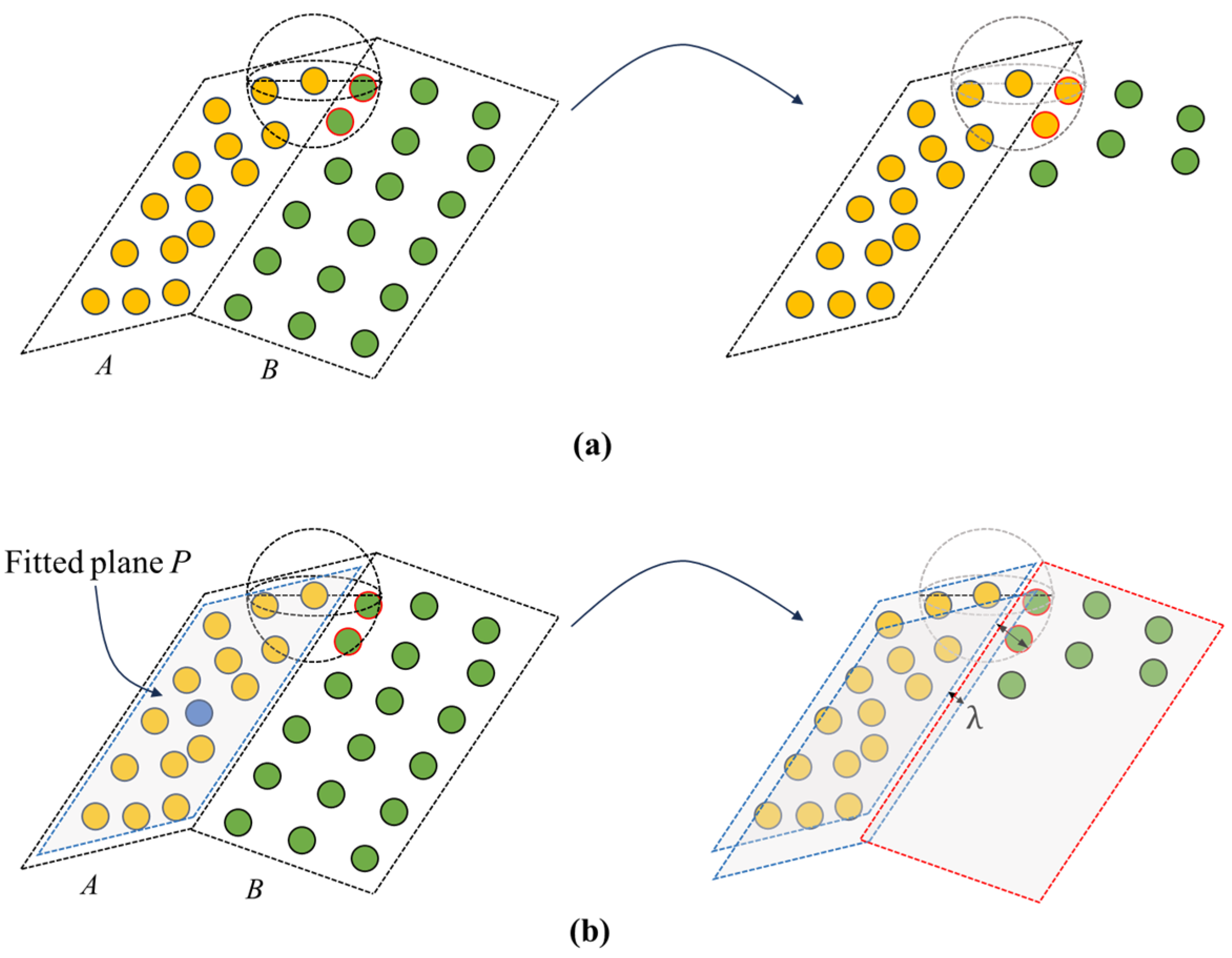
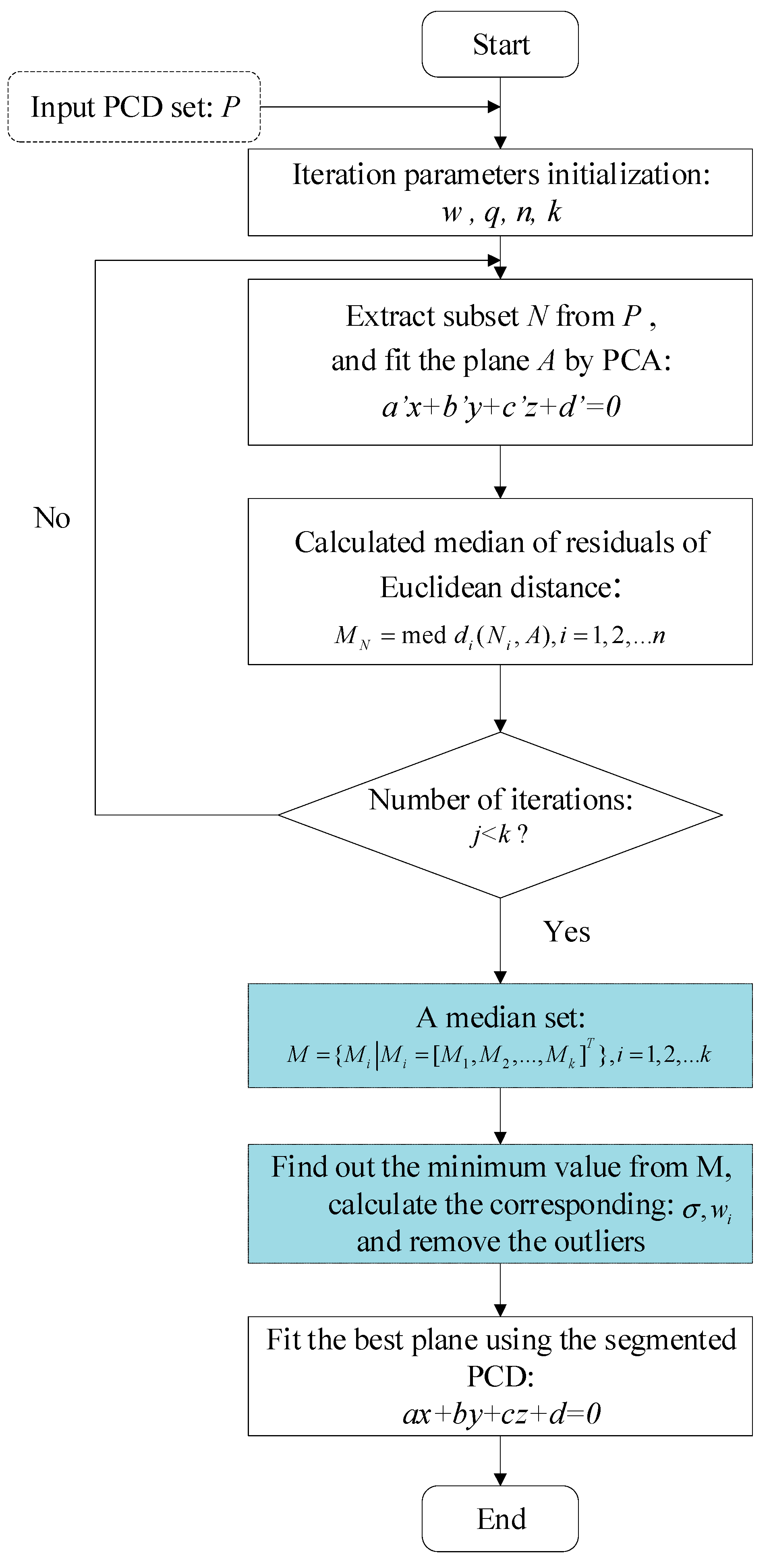
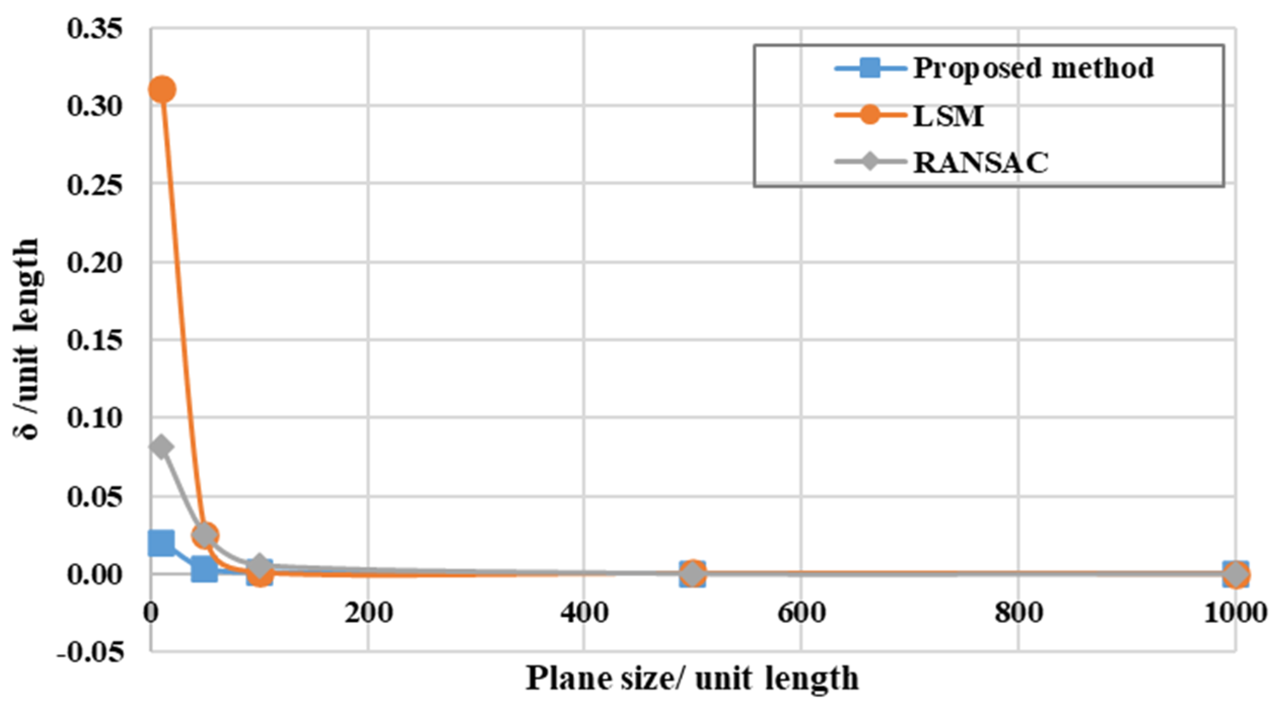
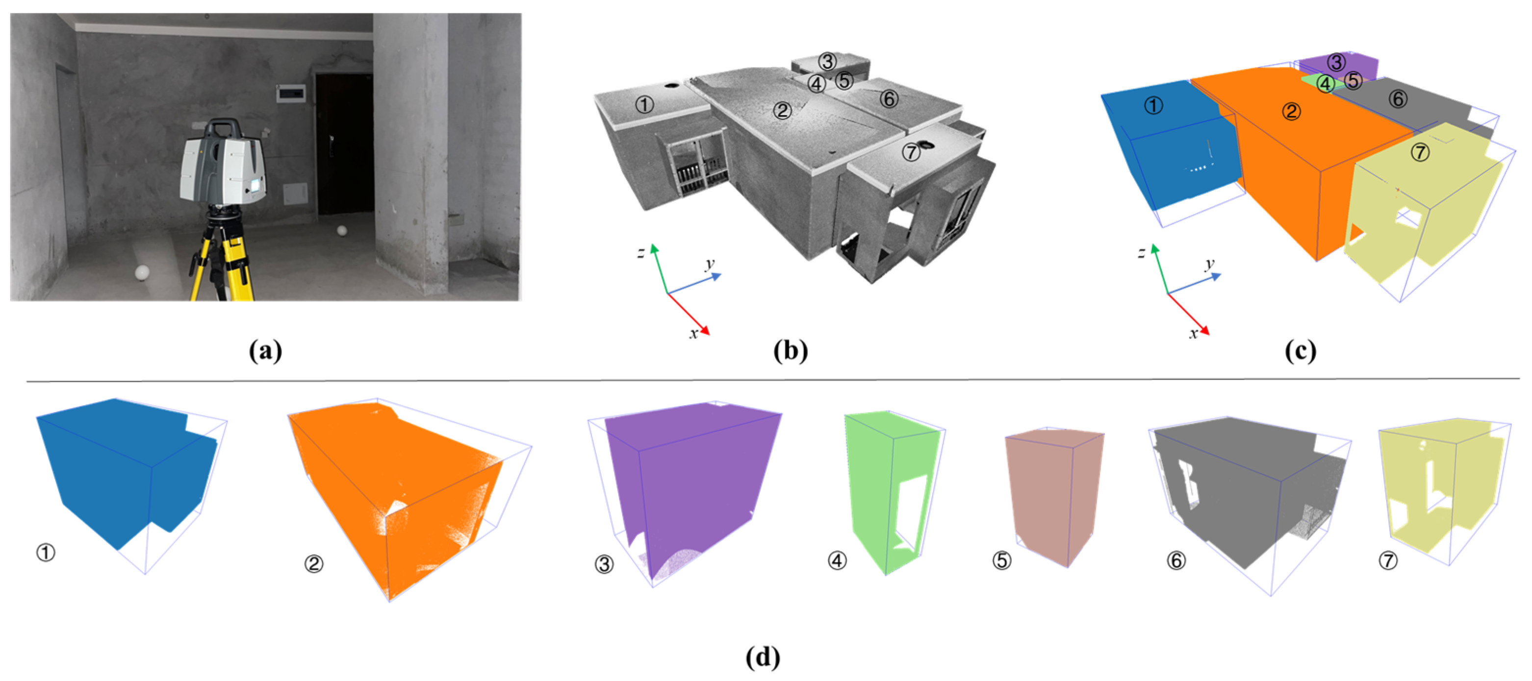
  • Surface segmentation and plane fitting. An improved DBSCAN algorithm is introduced in this study to segment various surfaces accurately by introducing the additional processes of plane validation and coplanar parameter. Moreover, a slide window-based sampling method is applied to obtain the sample PCD for SQE. Then a revised Least Squares Method (LSM) algorithm is proposed to remove the outliers and obtain the best-fitted reference plane for the later processes.
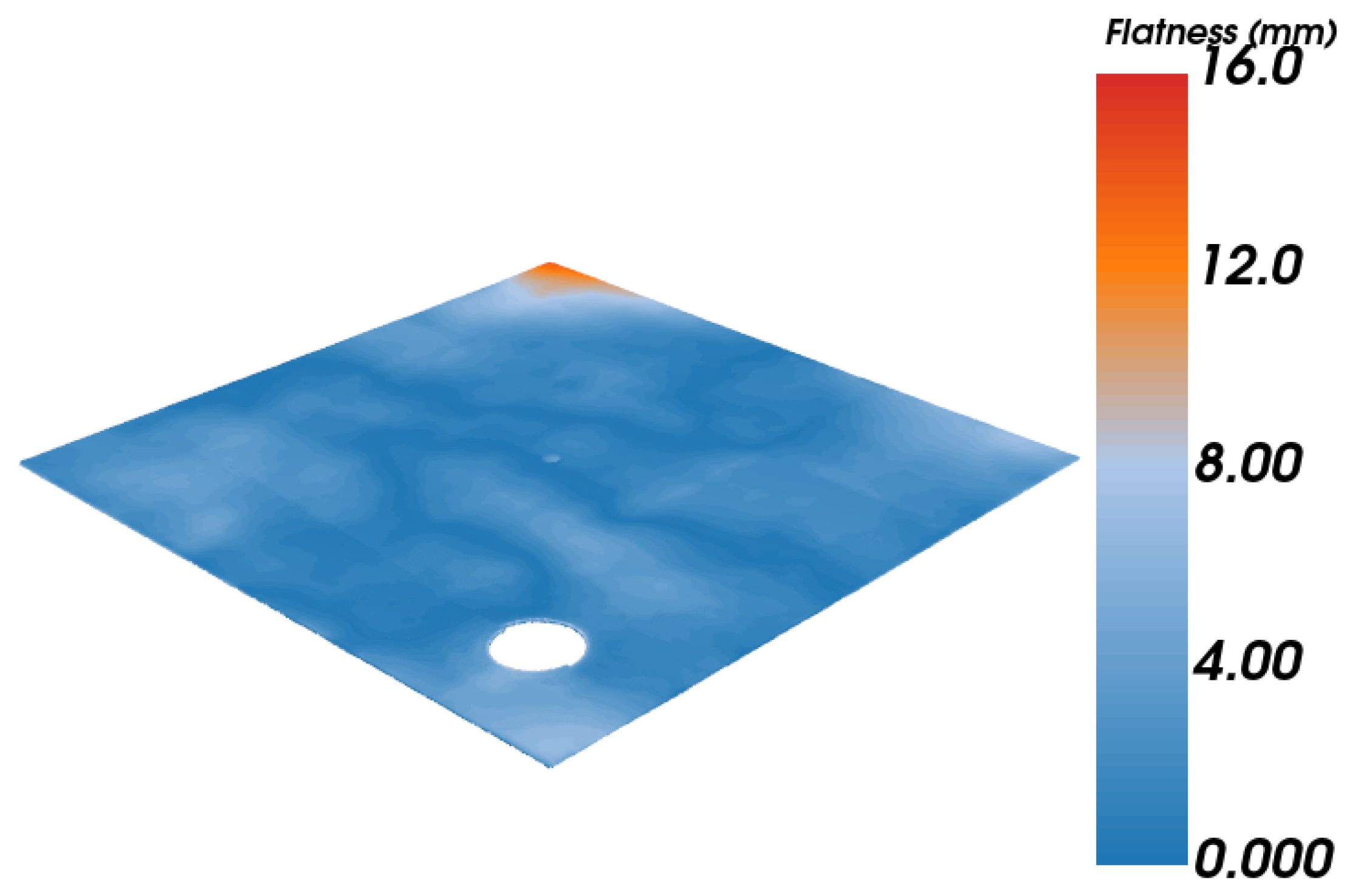
  • Automated SQE and result visualization. The flatness, verticality, and squareness evaluation are performed based on the reference plane, and a color-coded map is produced for a clear visualization.

3.1. Data Preparation

Since laser scanning is an application-oriented technique in the construction industry, it is important to ensure that the acquired PCD data meet the requirements of the application. Therefore, several factors need to be taken into account for scanner and parameter determination [1,53]:
Tolerance is the most important factor as indicated in Figure 4, which indicates the limitation of the acceptable value of specific measurement, decided by the measurement purposes and standard requirements. For instance, the verticality tolerance in ACI-ITG-7M [9] is 6/3000 mm; this requires the resolution of the scanner should be less than 6 mm at the distance of 3 m, taking 0.6~1.2 mm normally in practice for better results. This is the first criterion that needs to be considered, which will affect the selection of the scanner and the factors afterwards.
Resolution is the second factor, referring to the minimum size of each neighboring point, which determines the quality of the PCD directly. In simplified terms, the resolution of the scan is the largest value of measurement accuracy, scan density, and beam diameter at the front window. The determination of resolution in each scan should combine the requirement of tolerance with the scanner product specifications, and then select the maximum resolution that meets the tolerance requirements, but generally no more than 1/5 of the tolerance.
Range is the distance between the objective and the scanner; the maximum range is determined by the scanner source and energy. According to [1], the TOF laser scanners have a longer maximum range (up to 6000 m) compared to phase-shift laser scanners. The scanning range is estimated depending on the working condition, and then determined by combining it with the resolution and scanning mode of the scanner. Normally, the quality of the PCD will decrease with the increase in scanning range.
Scanning time is the parameter that depends on the resolution, scanning range, and objectives, which is also an important point for balancing efficiency and accuracy in practice. It should be considered by the experienced expert who performs the measurement process.
To obtain an optimal parameter setting for indoor PCD acquisition, several scanning tests were performed by scanning a concrete plate in different distances in the lab. The selected scanner is Leica P50 in this study, which was used in many research works [54,55,56], with a high-speed scan rate (1 million points/s), low noise range (maximum 0.4 mm at 10 m), and large measurement range (0.4 m–>1000 m). The corresponding results are shown in Table 2 and visualized in Figure 5. It can be seen that the scanning efficiency is linear, decreasing with the increase in scanning range when the resolution is fixed. When the required resolution is higher, the scanning time dramatically increases for a larger scanning range. Therefore, in most cases where the scanner is pre-determined in practice, a feasible parameter determination process should be as the following to balance the accuracy and efficiency: (1) determine the tolerance according to the project requirements, and thus find out the resolution limits; (2) the range is then decided according to the measurement conditions on site; (3) select the optimal mode based on the resulting scanning time–range curves.
For indoor elements’ SQE in this study, the evaluation tolerance for indoor element surface quality evaluation ranges from 5–8 mm, which requires that the resolution of the scanner should ideally be under the order of this magnitude. Furthermore, the measurement distance is around 10 m inside the building; mode 7 and 8 are suitable for indoor element scanning if a high-quality PCD is required. However, mode 13 and 14 are also acceptable for the cost, time, and quality effective in practice.
When the measurement should be performed for outdoor components, such as façades, the modes 6, 12, or 18 are good for the data acquisition according to the tolerance level.
Obviously, the indoor components need to be subjected to multiple scans from several different locations for a complete data collection. Then, the point clouds from each different station are registered to a unified coordinate system. The original data of the indoor elements should then be de-noised to eliminate the points that do not belong to the elements’ surface.

3.2. Surface Segmentation and Plane Fitting

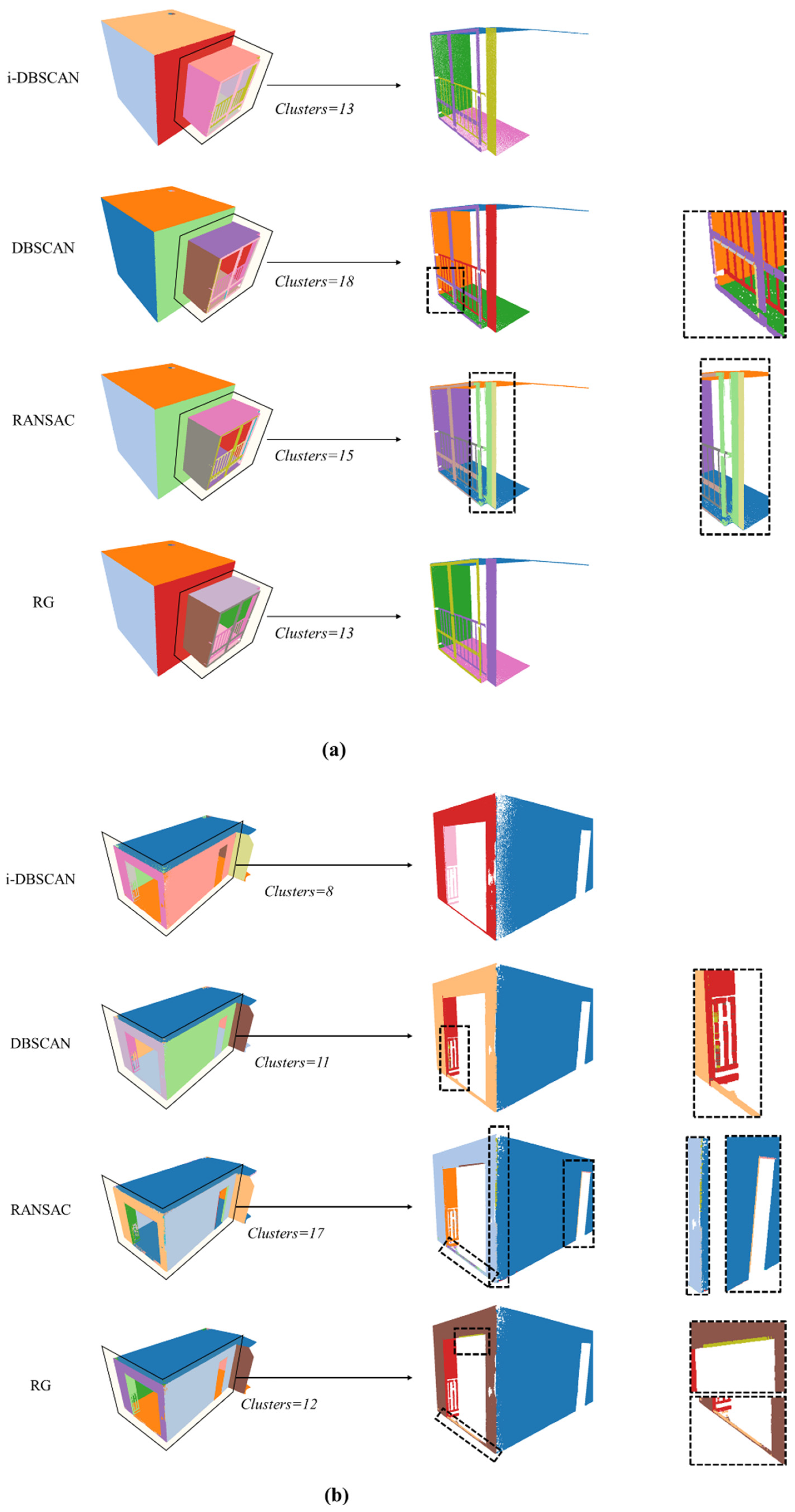
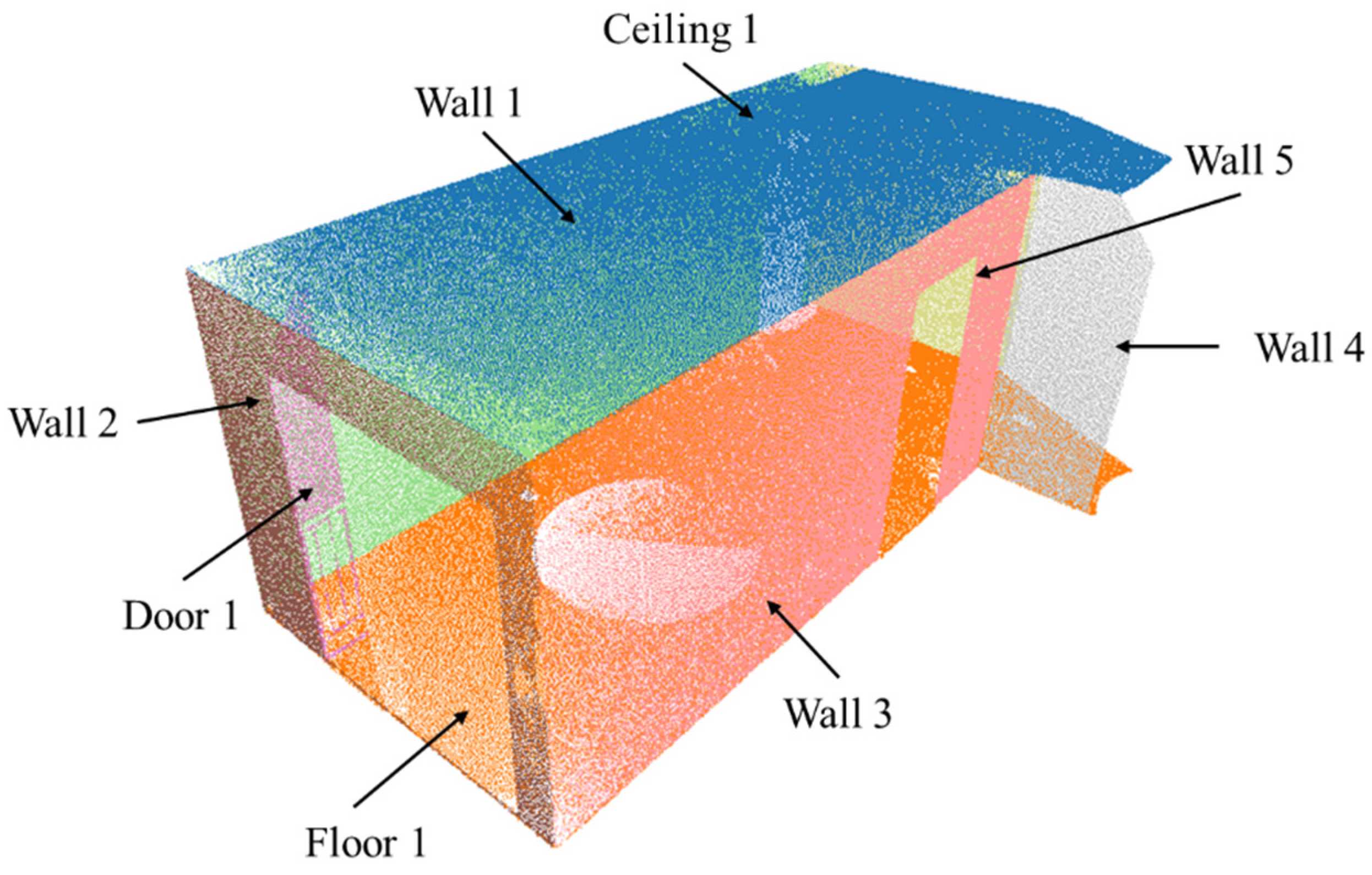
3.2.1. Surface Segmentation Based on Improved DBSCAN

As a crucial step for the proposed method, the segmentation of surfaces from different structural components plays an important role in the accuracy of the following SQE. Within this study, an improved DBSCAN (i-DBSCAN) is proposed to facilitate the multi-plane PCD segmentation and make the boundary detection more robust. The main pipeline of the proposed algorithm is shown in Figure 6.
Labeling of the points. Within the proposed method, the first step is to identify all the core points and label them, which is similar to the conventional DBSCAN. This is to prepare the input of the next step, for facilitating the sample points selection.
Sample points selection and plane fitting. This step is to select three potential points from the core points set to fit an initial plane. Apparently, the potential points should be the core point away from the intersections and boundaries of the PCD. The selection process is conducted as follows. Firstly, a core point ci within the test core point group and its k-nearest neighbors pij (j = 1, 2, … k) are input to initiate the process, and the distance matrix d i s t i is calculated within the group. And then the three farthest away points, (e.g., p i k , p i k 1 , p i k 2 , ), are selected as the potential candidate points based on the distance matrix. Next, the normal directional compatibility check needs to be conducted according to the following requirement:
1 3 j = k 2 k cos ( n ¯ c i , n ¯ p i j ) < 1 k j = 1 k cos ( n ¯ c i , n ¯ p i j )
where n ¯ c i , n ¯ p i l , n ¯ p i l + 1 , n ¯ p i l + 2 represent the normal vector of core point ci and potential points p i l ,   p i l + 1 ,   p i l + 2 , respectively, and n ¯ p i j denotes the normal vector of the j-th k-nearest neighbors. By doing the above check, it can ensure that the normal directions of the three selected points are essentially compatible with the average normal direction of all points in this k-neighborhood.
After passing the compatibility test, the fitting plane is generated based on the three potential candidate points selected above, which can be described as follows:
P : A x + B y + C z + D = 0
where A , B , C denote the components in x, y, z directions of the unit normal vector of plane P, while D represents the normal distance of the plane to the origin of the coordinate system.
The sample point selection process starts from the first core point in the labeled set of core points until three sample points that meet the requirement are found, which can be immediately followed by plane fitting and the next step of plane validation. If the three sample points cannot meet the requirements of Equation (2) or the subsequent planar validation fails, the process returns to the next core point and starts again.
Plane validation. It is clear that the fitted plane based on the three core points selected above should have as small a distance as possible from the nearby points within the entire sample. Therefore, the plane validation is proposed here to verify the validity of the fitted plane.
Firstly, the distance d m , ( m = 0 , 1 , , k ) between plane P and core point group p i j ( j = 1 , 2 , k ) are calculated, resulting in a distance matrix D = { d 0 , d 1 , , d k } . Following that, an analysis is conducted based on the mean value, μ , and standard deviation σ of the distance matrix D: if less than 25% of the core points within this group fall outside the range [ μ σ , μ + σ ] , the fitted plane P is valid, i.e., if r1 < r2, the further process can be conducted based on the plane F, where r 1 = c a r d { d m | d m μ + σ } ( m = 0 , 1 , k ) , and r 2 = 0.25 ( k 2 ) .
Clustering. Once a satisfied fitting plane P and the corresponding core point c i are determined, the clustering is able to be conducted based on the DBSCAN and a coplanar parameter, λ . If the point m of the multi-plane PCD is in the same cluster with core point c i , two requirements should be satisfied: (1) the point m is density-reachable of c i according to the theory of DBSCAN; and (2) the distance between point m to plane P is less than the coplanar parameter λ , while λ is defined as follows:
λ = μ + a σ
where a is defined as below:
a = { 1.5 + 2 ( r 2 r 1 ) ,   w h e n : r 2 > r 1 0 , w h e n : r 2 r 1
As indicated above, when r 2 > r 1 , it indicates that less than 25% of the total points are far away from the plane, which results in a wider range for the coplanar parameter λ . On the contrary, the coplanar parameter λ is set as the mean value of distance matrix D as the last step says.
As shown in Figure 7, the traditional DBSCAN may cluster the point from plane B into the group with plane A due to the intersection of the two planes and the density difference. With the proposed DBSCAN algorithm in this study, by fitting a valid plane and introducing the corresponding coplanar parameter, it overcomes the mis-clustering problem of the traditional DBSCAN at the junction of multiple planes, thus improving the accuracy of the plane clustering.

3.2.2. Plane Fitting

This step plays an important role in the final flatness results since the fitted plane is the reference for the deviation calculation, which determines the accuracy of the flatness result. The previous work [4,23] used the Least Squares Method (LSM) to fit the plane, which is efficient and good for PCDs with less noise and fewer points, but could be affected by the local outliers. Within this study, the outliers are the part that needs to be measured. Therefore, an improved algorithm is proposed to better fit the plane using the Least Median of Squares, (LMedS), and the flowchart is shown in Figure 8.
Step 1: The testing surface sample PCD P = { P i | P i = [ x i , y i , z i ] T } is input and the initial parameters, w, p, n, q, are determined according to the following formulas based on LMedS:
k = lg ( 1 q ) lg ( 1 w n )
where k is the minimum iteration number, q is the possibility to obtain a good subset form P (generally taken as 0.95–0.99), n is the sample point number for calculating the plane model (for plane fitting, min n = 3), and w indicates the proportion of inlier points in the sample, normally more than 50% for LMedS.
Step 2. Extract a subsample N = { N i | N i P , i = 1 , 2 , n } from P, and fit a plane A, a’x + b’y + c’z + d’ = 0, by means of the PCA method. Then the median of the residuals of the Euclidean distance of each point in subsample N from the fitted plane A is determined, denoted by M N = med   d i ( N i , A ) , i = 1 , 2 , n .
Step 3. Repeat steps 2–3 until the number of iterations is reached to k, record the set of the median value M = { M i | M i = [ M 1 , M 2 , , M k ] T } , i = 1 , 2 , k , from which find out the minimum value, denoted by M M . Afterwards, the robust standard deviation σ and weight w i are determined to segment the outliers and inliers for the sample as Equations (7) and (8) say, and the final plane, F: ax + by + cz + d = 0, is fitted based on the segmented PCD.
σ = 1.4826 × ( 1 + 5 n p ) × M M
w i = { 1 , | d i | σ 2.5 0 , | d i | σ > 2.5
where M M indicates the minimal among the median set, M, and di indicates the Euclidean distance of point Pi in sample P, and w i means the weight for point P i in sample P.
The proposed method overcomes the effect of outliers, and also overcomes the dependence of the RANSAC method on the threshold and iteration period.
Experiments were performed to validate the feasibility and robustness. Python tool was used to generate 1000 points which belong to the plane with the size of 10 × 10 expressed as Equation (9), and 100 Gaussian noise points with a mean value of 0 and standard deviation of 3.0 were added as outliers:
P :   x + 2 y z + 1 = 0 ,   x , y [ 10 , 10 ]
Table 3 presents the average fitting results of the points defined above by three different fitting algorithms after being repeated 50 times, with the reference parameters of plane P: a = 0.4082, b = 0.8165, c = −0.4082, and d = 0.4082. From the results, it can be seen that the parameters fitted by the three compared methods are all close to the predefined parameters when the data do not have outliers, and the standard deviation (δ) of the distance of each point to the respective fitting plane is close to 0. When fitting the data with outliers, the parameters fitted by the proposed method are the closest to the predetermined parameters, and present the smallest δ value, which also demonstrates its robustness.
The plane size also has an effect on the fitting results, which was analyzed by fitting the plane with different size values but the same Gaussian noise points (with a mean value of 0 and standard deviation of 3.0); the results are shown in Figure 9. It can be seen that the proposed method has the smallest value of δ when the size is small (10 × 10); δ also converges rapidly when the size increases. This also proves the robustness of the proposed method, which significantly improves the accuracy of plane fitting regardless of the size.
Afterwards, the normal vector of the sample surface can be determined based on the equation of plane F, whose direction coincides with the vector pointing in the direction of the interior.

3.3. SQE Based on PCD

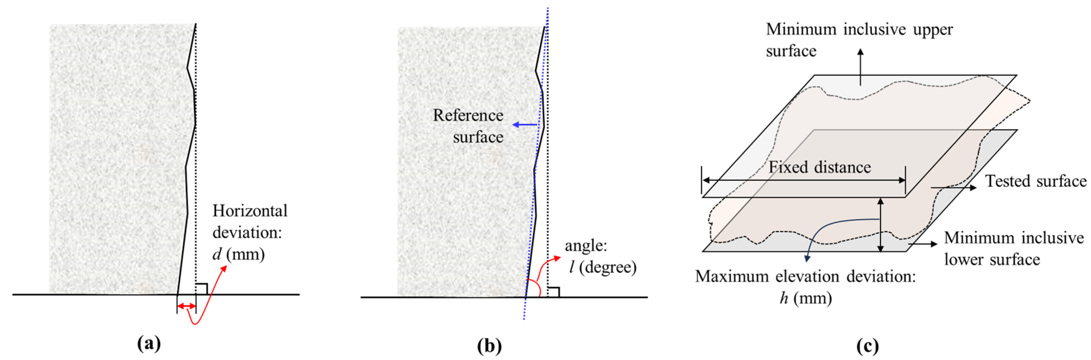
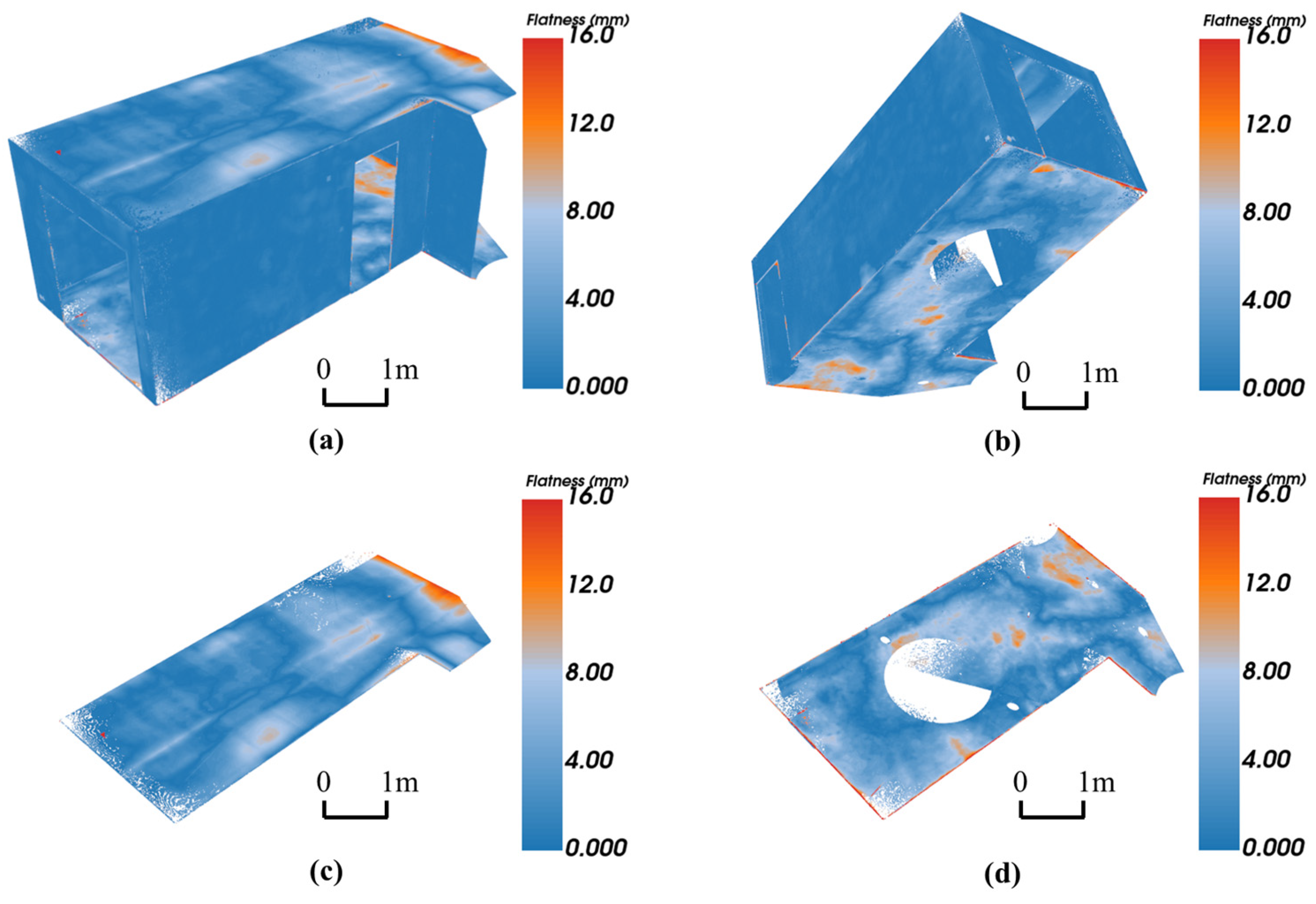
3.3.1. Flatness Evaluation (FE)

After the plane is obtained, the local flatness of the corresponding sample can be evaluated based on the deviations between the fitted surface and sample points. The distance matrix from point P ( x p , y p , z p ) in the sample PCD to the plane F is calculated using Equation (10), and a deviation map is generated to visualize the testing results (Figure 10).
Within the map, a threshold h is set, consistent with the standard [5] to facilitate the representation of the amount of deviation at different locations, which is valuable for the following repairing work.
d p = | a x p + b y p + c z p + d | a 2 + b 2 + c 2

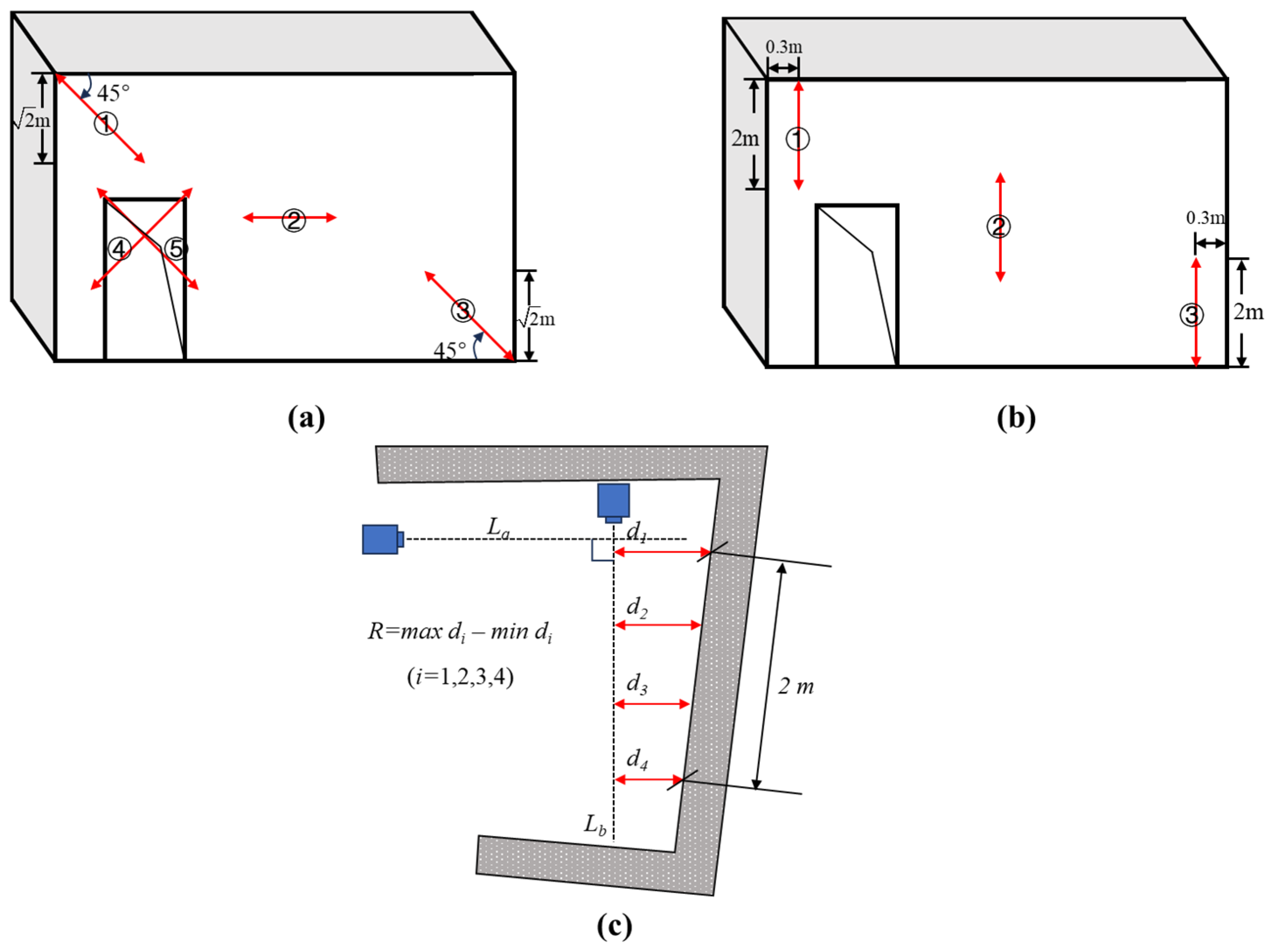
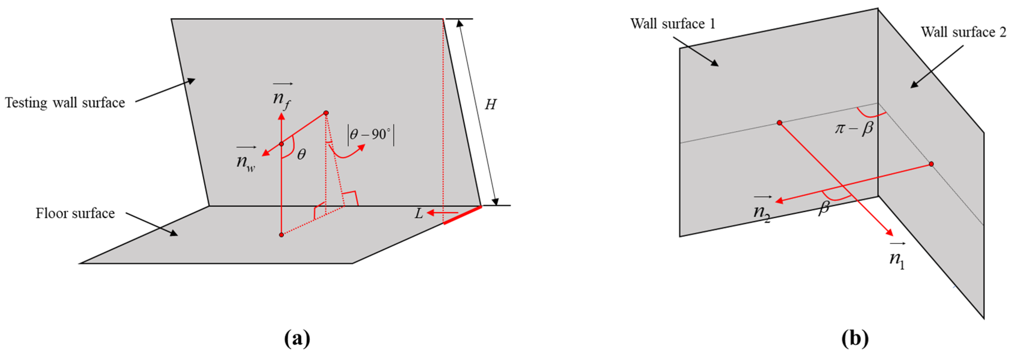
3.3.2. Verticality Evaluation (VE)

According to the summary in Section 1, the verticality evaluation in practice mainly uses the horizontal deviation method, and thus the full height of the testing elements should be measured. Within this study, the boundary detection was achieved according to the RANSAC algorithm because of the relatively simple geometry of the PCD edge. After that, the dimensions of the elements are easy to obtain using the detected edge line.
In practice, the verticality assessment is mainly tested for vertical elements, e.g., walls, columns, etc. Therefore, the method used in this study is also mainly applicable to vertical walls. As shown in Figure 11a, the normal vector of the tested wall, n w , and floor surface, n f , are obtained as introduced in Section 3.2.2, and the verticality L can be evaluated using n w and n f as follows:
L = H sin ( | arccos ( n w n f | n w | × | n f | ) π 2 | )

3.3.3. Squareness Evaluation (SE)

In practice, the squareness of a room is measured through a series of complicated manual operations, and the results are influenced by a number of factors as Section 1 stated. The flatness evaluation process has found the best-fitted plane of the wall with the methodology as indicated in Section 3.2.2. As shown in Figure 11b, the squareness can be assessed using the angle between two normal vectors of the testing walls:
S = π β = π arccos ( n 1 n 2 | n 1 | × | n 2 | )
Apparently, the closer angle β is to 1 2 π , the better the squareness of the room is. According to the upper limits of R mentioned in Section 1, the tolerance of β is 0.001592 π , i.e., the angle β should be in the range of ( 1 2 ± 0.001592 ) π .

4. Experiment Validation

In order to verify the feasibility of the proposed method in this study, experiments were conducted on a real residence building. The data collection and pre-processing are discussed in Section 4.1, and the segmentation of the surface PCD is given in Section 4.2. Then the separated PCD is sampled and fitted to the plane, and the automatic flatness, verticality, and squareness evaluation are finished in Section 4.3.

4.1. Data Collection and Pre-Processing of PCD

One apartment with seven rooms in total was scanned by Leica P50 (shown in Figure 12a), with the scanning mode 14 used in this study based on the analysis in Section 3.1. In order to obtain the comprehensive PCD data, six scans were performed, taking a total of 35 min including the setting of the scanner.
After the on-site scanning, the row data with 8.36 × 10⁹ points are imported into the software “Cyclone REGISTER 360”, which automatically registers the data by searching the target balls in the separated PCDs. It should be noticed that the coordinates of the PCD should be transferred.
Before conducting the segmentation, the PCD has to be de-noised due to the useless points contained in the scanning, e.g., the outdoor objects scanned through the windows or doors. Manual work is done within this process to remove the outliers and minimize the effects of them. Then, the PCD is subsampled using the Octree method due to the regularity of the PCD of building structures, in order to improve the calculation efficiency afterward, leading to a PCD with 5.4 × 10⁷ points in total as shown in Figure 12b.

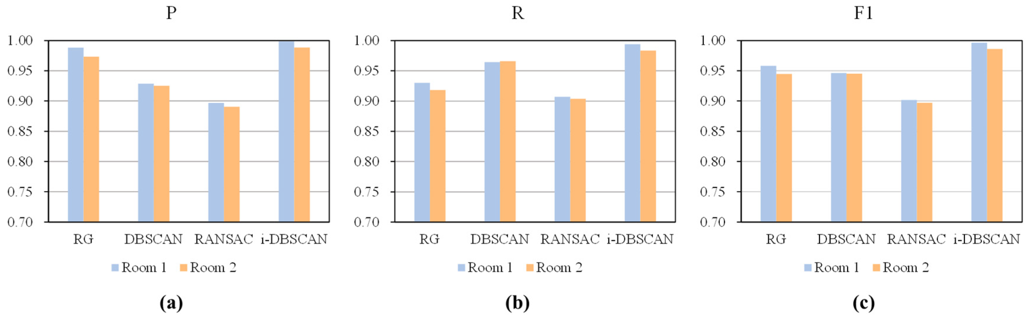
4.2. Surface Segmentation

Once the as-built PCD is prepared, the K-means cluster algorithm is utilized to cluster the PCD as separate rooms. As shown in Figure 12c, the testing PCD of the apartment was clustered and seven rooms were separated from the integrated PCD, which were rendered in with different colors.
After that, the segmentation procedure of the surfaces was conducted according to the method discussed in Section 3.2.1. In order to evaluate the segmentation quality, several common metrics, Precision (P), Reall (R), and F1-score, are used in the study as defined below:
P = T P T P + F P R = T P T P + F N F 1 = 2 P R P + R
where TP is the (True Positives) number of points found in both the ground-truth cluster and segmented cluster; FP (False Positive) indicates the number of points found in the segmented cluster, but not found in the ground-truth cluster; while FN (False Negative) is the number of points not found in the segmented cluster but found in the ground-truth cluster.
Taking Room 1 and Room 2 as examples, three different algorithms, including traditional DBSCAN, RANSAC, and Region Growing (RG), are compared with the proposed i-DBSCAN algorithm; the clustered surfaces results are displayed in different colors as shown in Figure 13. In Figure 13a, the first column displays the surface clustering results of Room 1, while the second column zooms in on the clustering results of windows because of the complex geometrical structures. The results indicate that all the algorithms could correctly segment the main planes (walls, ceilings, floors, etc.) of the room. However, the PCD of the window part is more challenging for the clustering due to the presence of railings and window frames. The results of the DBSCAN and RANSAC algorithms show that the PCDs at the intersections of multiple planes are recognized as outliers, resulting in the segmentation of PCDs that should belong to the same plane into different clusters (as indicated in the third column). This results in the DBSCAN and RANSAC algorithms segmenting more clusters than actually exist. Comparatively, the RG algorithm not only detects the planes correctly, but also properly clusters the window frames and railings in the right clusters. A similar pattern is observed in Figure 13b; RANSAC tends to recognize boundary points as a separate cluster and results in a low recall rate. On the contrary, the proposed i-DBSCAN algorithm in this paper accurately recognizes the boundary points and clusters them into the right segment because of the introduced seed plane and coplanar check.
Figure 14 indicates the evaluation metrics of the different segmentation approaches on the tested PCDs. It is clear that all the compared methods have obtained a high score of P, which demonstrates that the compared methods have good precision in the detection of inlier points of the plane, with RG and i-DBSCAN being the highest. Compared with the others, the proposed approach in this study has obtained the highest R and F1 scores, indicating the proposed approach is able to detect the true points belonging to the plane. Although the time cost of the proposed method is longer than the compared ones, it improves the accuracy level in planar point detection (especially the judgment of boundary points), which helps greatly for the following SQE process.

4.3. Automatic SQE Results

In the experiment, the PCD of Room 2 was chosen as the testing data to validate the flatness evaluation. The segmented data of Room 2 have five walls, one floor, one ceiling, and one door as shown in Figure 15. Then all the surfaces of this room were subjected to the SQE using the proposing methodology.

4.3.1. Flatness Evaluation Results

After the surfaces are sampled, the planes are fitted and the flatness is evaluated according to the methodology of Section 3.2, where the procedures of Room 2 are discussed in detail here as an example.
According to the methodology in Section 3.2, the point cloud of each surface is taken as input and its best plane is fitted to obtain the plane parameters as shown in Table 4. The height deviation of each point cloud from the corresponding fitted plane was then calculated and visualized, and the results are shown in Figure 16.
As can be seen from Figure 16a,b, the flatness of the walls in Room 2 meets the requirements overall, although there are some boundary areas that exceed the threshold when it is set to 8 mm. However, the calculation results for the ceiling show that the flatness does not satisfy the specification at its middle zones and boundary with the wall (see Figure 16c), with a maximum value of 21.6 mm. The situation for the floor (see Figure 16d) is also similar to that of the ceiling. This is due to the fact that the formwork of the horizontal elements needs to bear a large self-weight when the concrete is poured and is also prone to deformation at the connection with the wall formwork. The data in Table 4 confirm this conclusion: approximately 95.36% and 89.21% of all points on the floor and ceiling meet the allowable tolerances, indicating that they did not meet the requirements for as-built acceptance in the flatness evaluation and that subsequent repair work is required. Note that the noise points did not affect the flatness evaluation results since the plane fitting procedure takes them as outliers and removes them when fitting the plane. However, it will affect the absolute value of the maximum distances (known as Max. dist in the table).

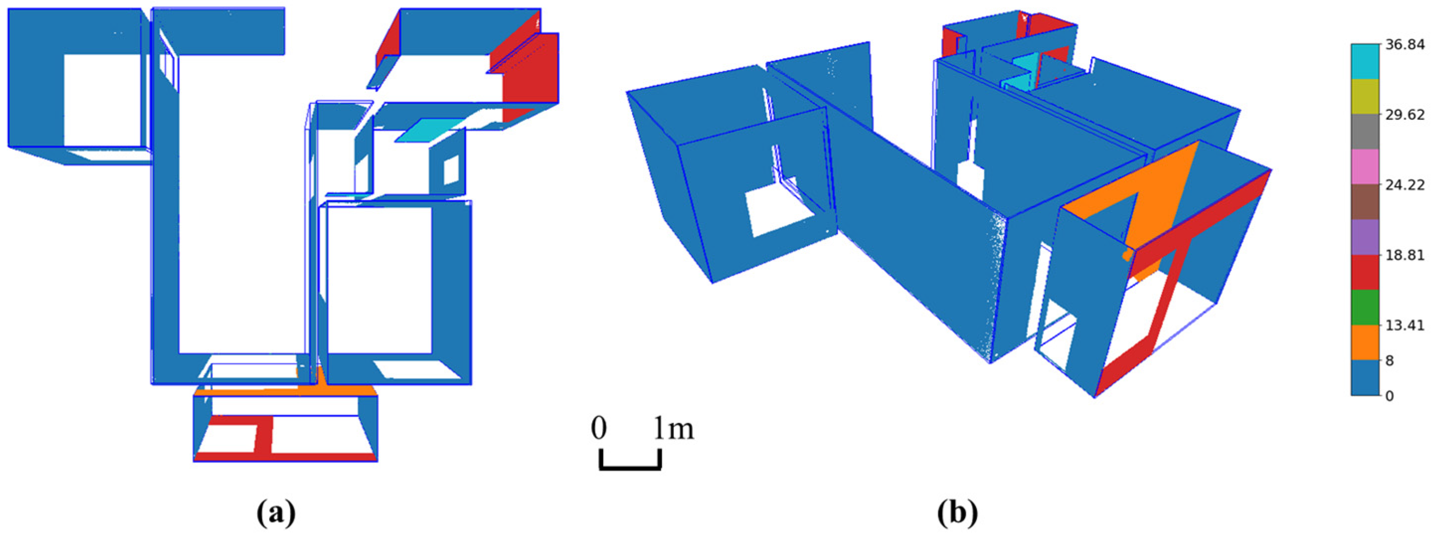
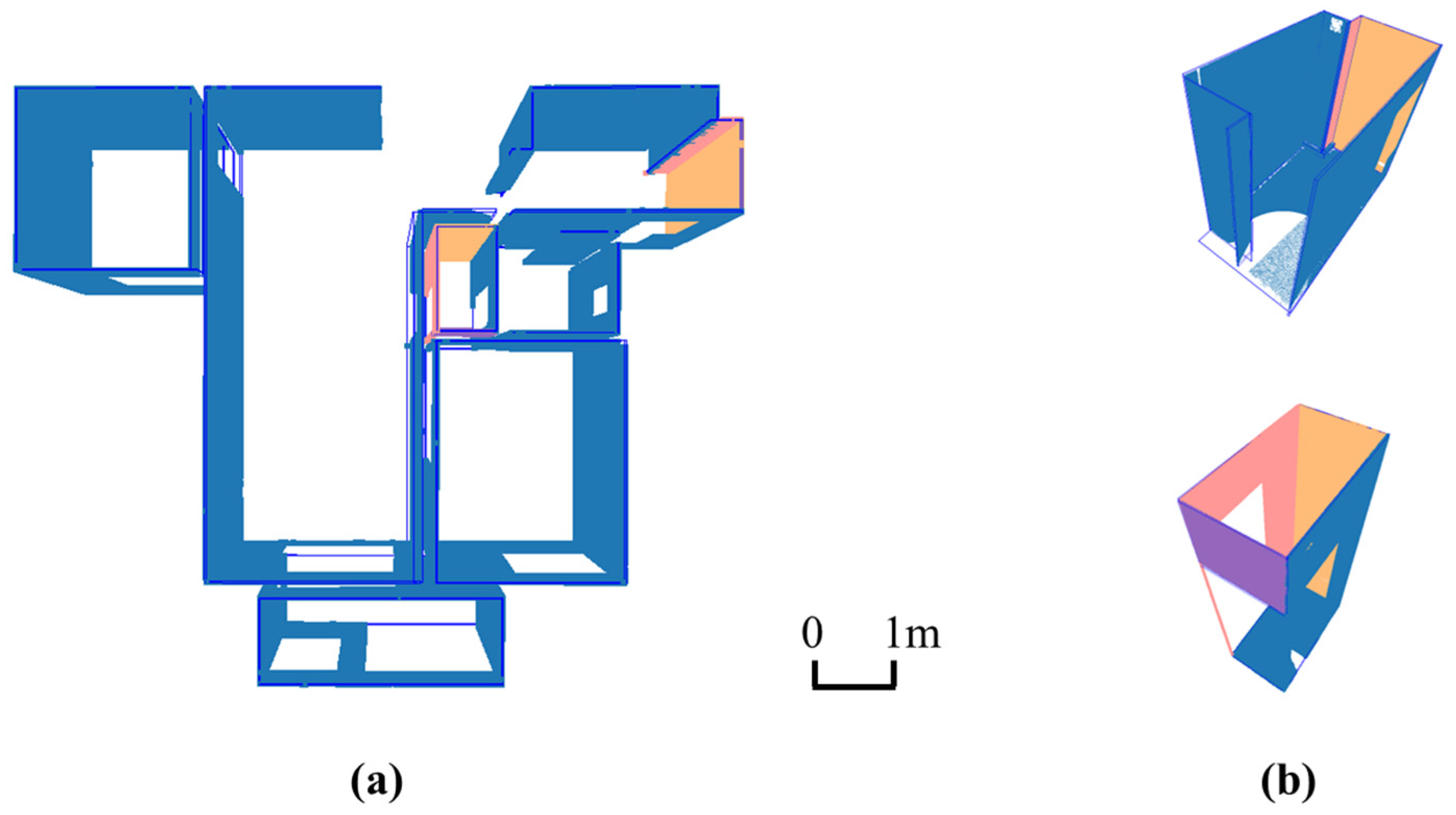
4.3.2. Verticality and Squareness Evaluation Results

The results of the walls’ verticality and squareness for the entire residential building are shown in Figure 17. It is clear that the vertical walls in Rooms 1, 2, 5, and 6 are satisfied. Taking 8 mm as the tolerance of verticality, Rooms 3, 4, and 7 have two walls, two walls, and two walls, respectively, that do not meet the verticality requirements. The locations of them are displayed in the color-coded map in Figure 17, which reveals that most of the walls that do not meet the requirements are found in small spaces such as the kitchen, bathroom, and terraces. The detailed verticality results of the other rooms are shown in Table 5.
Similarly, the squareness of the room is calculated based on the method in Section 3.3, and the results are displayed in Figure 18 and Table 6. It can be seen that the squareness between wall 5 and wall 6 in Room 3, and between wall 2 and wall 3 in Room 4, as well as between wall 3 and wall 4 in Room 4, does not fulfill the requirements. Obviously, wall 5 and wall 6 in Room 3 are two small walls that cover the flue in the kitchen, which is the secondary structure after the main frame structure was formed. Therefore, the verticality problem can easily occur during construction. Similarly, Room 4 is a bathroom, which is only 1.35 m2 in size, making it more difficult for the formwork and therefore prone to this problem.

5. Conclusions

Concrete surface quality is the key procedure for as-built acceptance testing, which requires an automated system that can facilitate the measuring processes, as well as provide recognizable visualizations. This study proposed a framework for indoor SQE based on point cloud.
Within this research, an improved DBSCAN algorithm is proposed to better segment the building surface from the PCD, by fitting a valid plane and introducing the corresponding coplanar parameter to overcome the mis-clustering on boundary points. Furthermore, a LMedS-based plane fitting algorithm is developed to find out the best fitting plane of the surface PCD and minimize the effect of outliers on the plane fitting. Subsequently, the flatness, verticality, and squareness evaluation of the building are calculated based on fitted planes. The results are indicated with a color-coded deviation map, which allows easy visualization and the finding of areas that do not satisfy the acceptance standards.
The validation tests on the virtual surfaces and real building data of an apartment demonstrate that the proposed algorithms can improve the accuracy of surface segmentation and plane fitting compared with traditional model fitting algorithms, which is conducive to enhancing the reliability of SQE results. The proposed system is able to provide overall information of the surface quality, including flatness, verticality, and squareness of a residential building, thus improving the informatization and comprehensiveness of it.
In the future, a deep study of other SQE indexes should be conducted to enrich the acceptance system. And the BIM model can be introduced as a reference for SQE and as a storage carrier for results in order to realize the integration of the whole life cycle of the building.

Author Contributions

Conceptualization, D.C.; Methodology, S.C; Investigation, S.C., M.W., H.W.; Formal analysis, S.C., M.W., H.W.; Validation, N.S., Y.Z., and Y.D.; Data curation: K.H.; Writing—original draft, D.C.; Writing—review & editing, D.C., K.H. and X.H.; Project administration, Y.Z.; Funding acquisition, X.H. All authors have read and agreed to the published version of the manuscript.

Funding

This research received no external funding.

Data Availability Statement

Data are contained within the article.

Conflicts of Interest

Authors Dongbo Cai, Shaoqiang Chai, Mingzhuan Wei, Hui Wu, Nan Shen was employed by the company Seventh Engineering Bureau, CCCC Frist Highway Engineering Group Co., Ltd. and Author Yanchao Ding was employed by the company Huasheng Testing Technology Co., Ltd. The remaining authors declare that the research was conducted in the absence of any commercial or financial relationships that could be construed as a potential conflict of interest.

References

  1. Kim, M.-K.; Cheng, J.C.P.; Sohn, H.; Chang, C.-C. A framework for dimensional and surface quality assessment of precast concrete elements using BIM and 3D laser scanning. Autom. Constr. 2015, 49, 225–238. [Google Scholar] [CrossRef]
  2. Construction Industry Institute (CII). RS203-1—Making Zero Rework A Reality; Construction Industry Institute (CII): Austin, TX, USA, 2005. [Google Scholar]
  3. Mills, A.; Love, P.E.; Williams, P. Defect costs in residential construction. J. Constr. Eng. Manag. 2009, 135, 12–16. [Google Scholar] [CrossRef]
  4. Li, D.; Liu, J.; Hu, S.; Cheng, G.; Li, Y.; Cao, Y.; Dong, B.; Chen, Y.F. A deep learning-based indoor acceptance system for assessment on flatness and verticality quality of concrete surfaces. J. Build. Eng. 2022, 51, 104284. [Google Scholar] [CrossRef]
  5. Sameer, G.; James, G.; Burcu, A.; Scott, T.; Chris, P. Running Surface Assessment Technology Review; Carnegie Mellon University: Pittsburgh, PA, USA, 2002. [Google Scholar]
  6. GB50204-2015; Standard, Code for Acceptance of Construction Quality of Concrete Structures. China Building Industry Press: Beijing, China, 2015.
  7. Tan, Y.; Li, S.; Wang, Q. Automated Geometric Quality Inspection of Prefabricated Housing Units Using BIM and LiDAR. Remote Sens. 2020, 12, 2492. [Google Scholar] [CrossRef]
  8. MNL-135; Tolerance Manual for Precast Concrete Construction. American Standard: Piscataway, NJ, USA, 2000.
  9. ACI ITG-7-09; Specification for Tolerances for Precast Concrete. American Standard: Piscataway, NJ, USA, 2009.
  10. EN 13670:2009; Execution of Concrete Structures. European Standard: Brussels, Belgium, 2009.
  11. Zhao, W.; Jiang, Y.; Liu, Y.; Shu, J. Automated recognition and measurement based on three-dimensional point clouds to connect precast concrete components. Autom. Constr. 2022, 133, 104000. [Google Scholar] [CrossRef]
  12. Wang, Q.; Kim, M.-K.; Cheng, J.C.; Sohn, H. Automated quality assessment of precast concrete elements with geometry irregularities using terrestrial laser scanning. Autom. Constr. 2016, 68, 170–182. [Google Scholar] [CrossRef]
  13. Ordóñez, C.; Martínez, J.; Arias, P.; Armesto, J. Measuring building façades with a low-cost close-range photogrammetry system. Autom. Constr. 2010, 19, 742–749. [Google Scholar] [CrossRef]
  14. Kashani, A.G.; Crawford, P.S.; Biswas, S.K.; Graettinger, A.J.; Grau, D. Automated tornado damage assessment and wind speed estimation based on terrestrial laser scanning. J. Comput. Civ. Eng. 2014, 29, 04014051. [Google Scholar] [CrossRef]
  15. Zhou, Z.; Gong, J.; Guo, M. Image-based 3D reconstruction for posthurricane residential building damage assessment. J. Comput. Civ. Eng. 2015, 30, 04015015. [Google Scholar] [CrossRef]
  16. Wang, Q.; Kim, M.-K. Applications of 3D point cloud data in the construction industry: A fifteen-year review from 2004 to 2018. Adv. Eng. Inform. 2019, 39, 306–319. [Google Scholar] [CrossRef]
  17. Tang, P.; Huber, D.; Akinci, B. Characterization of Laser Scanners and Algorithms for Detecting Flatness Defects on Concrete Surfaces. J. Comput. Civ. Eng. 2011, 25, 31–42. [Google Scholar] [CrossRef]
  18. Bosch, F.; Guenet, E. Automating surface flatness control using terrestrial laser scanning and building information models. Autom. ConStruct. 2014, 44, 212–226. [Google Scholar] [CrossRef]
  19. BS 8204; Bases and In-Situ Flooring. British Standards Institution (BSI): London, UK, 2009.
  20. ACI 302.1R-96; Guide for Concrete Floor and Slab Construction. A.C.I. (ACI): Miami, FL, USA, 2004.
  21. ACI 117-06; Specifications for Tolerances for Concrete Construction and Materials and Commentary. A.C.I. (ACI): Miami, FL, USA, 2006.
  22. Bosché, F. Plane-based registration of construction laser scans with 3D/4D building models. Adv. Eng. Inform. 2012, 26, 90–102. [Google Scholar] [CrossRef]
  23. Li, D.; Liu, J.; Feng, L.; Zhou, Y.; Liu, P.; Chen, Y.F. Terrestrial laser scanning assisted flatness quality assessment for two different types of concrete surfaces. Measurement 2020, 154, 107436. [Google Scholar] [CrossRef]
  24. Cao, Y.; Liu, J.; Feng, S.; Li, D.; Zhang, S.; Qi, H.; Cheng, G.; Chen, Y.F. Towards automatic flatness quality assessment for building indoor acceptance via terrestrial laser scanning. Measurement 2022, 203, 111862. [Google Scholar] [CrossRef]
  25. Shih, N.-J.; Wang, P.-H. Using Point Cloud to Inspect the Construction Quality of Wall Finish. In Proceedings of the Architecture in the Network Society, Copenhagen, Denmark, 15–18 September 2004; pp. 573–578. [Google Scholar] [CrossRef]
  26. Nuttens, T.; Stal, C.; De Backer, H.; Schotte, K.; Van Bogaert, P.; De Wulf, A. Methodology for the ovalization monitoring of newly built circular train tunnels based on laser scanning: Liefkenshoek Rail Link (Belgium). Autom. Constr. 2014, 43, 1–9. [Google Scholar] [CrossRef]
  27. Bosch, F.; Biotteau, B. Terrestrial laser scanning and continuous wavelet transform for controlling surface flatness in construction–a first investigation. Adv. Eng. Inf. 2015, 29, 591–601. [Google Scholar] [CrossRef]
  28. Puri, N.; Valero, E.; Turkan, Y.; Bosché, F. Assessment of compliance of dimensional tolerances in concrete slabs using TLS data and the 2D continuous wavelet transform. Autom. Constr. 2018, 94, 62–72. [Google Scholar] [CrossRef]
  29. Neza, I.; Mohamed, M.I.; Syafuan, W.M. Surface Waviness Evaluation of Two Different Types of Material of a Multi-Purpose Hall Using Terrestrial Laser Scanner (TLS). IOP Conf. Ser. Mater. Sci. Eng. 2022, 1229, 012002. [Google Scholar] [CrossRef]
  30. Han, D.; Rolfsen, C.N.; Hosamo, H.; Bui, N.; Dong, Y.; Zhou, Y.; Guo, T.; Ying, C. Automatic detection method for verticality of bridge pier based on BIM and point cloud. In ECPPM 2021-eWork and eBusiness in Architecture, Engineering and Construction, Proceedings of the 13th European Conference on Product & Process Modelling (ECPPM 2021), Moscow, Russia, 15–17 September 2021, 1st ed.; CRC Press: Boca Raton, FL, USA, 2021; p. 6. [Google Scholar]
  31. Riveiro, B.; González-Jorge, H.; Varela, M.; Jáuregui, D.V. Validation of terrestrial laser scanning and photogrammetry techniques for the measurement of vertical underclearance and beam geometry in structural inspection of bridges. Measurement 2013, 46, 784–794. [Google Scholar] [CrossRef]
  32. Er’min, W.; Jiming, W.; Fei, Y.; Shengdeng, S.; Xuyang, Y. Detection of flatness and verticality of buildings based on 3D laser scanning technology. Bull. Surv. Mapp. 2019, 6, 85–88. [Google Scholar]
  33. Kim, M.-K.; Sohn, H.; Chang, C.-C. Automated dimensional quality assessment of precast concrete panels using terrestrial laser scanning. Autom. Constr. 2014, 45, 163–177. [Google Scholar] [CrossRef]
  34. Tang, X.; Wang, M.; Wang, Q.; Guo, J.; Zhang, J. Benefits of Terrestrial Laser Scanning for Construction QA/QC: A Time and Cost Analysis. J. Manag. Eng. 2022, 38, 05022001. [Google Scholar] [CrossRef]
  35. Ma, Z.; Liu, Y.; Li, J. Review on automated quality inspection of precast concrete components. Autom. Constr. 2023, 150, 104828. [Google Scholar] [CrossRef]
  36. Armeni, I.; Sener, O.; Zamir, A.R.; Jiang, H.; Brilakis, I.; Fischer, M.; Savarese, S. 3D Semantic Parsing of Large-Scale Indoor Spaces. In Proceedings of the 2016 IEEE Conference on Computer Vision and Pattern Recognition, Las Vegas, NV, USA, 27–30 June 2016; pp. 1534–1543. [Google Scholar] [CrossRef]
  37. Hu, X.; Zhou, Y.; Vanhullebusch, S.; Mestdagh, R.; Cui, Z.; Li, J. Smart building demolition and waste management frame with image-to-BIM. J. Build. Eng. 2022, 49, 104058. [Google Scholar] [CrossRef]
  38. Macher, H.; Landes, T. Grussenmeyer, From Point Clouds to Building Information Models: 3D Semi-Automatic Reconstruction of Indoors of Existing Buildings. Appl. Sci. 2017, 7, 1030. [Google Scholar] [CrossRef]
  39. Pu, S.; Vosselman, G. Knowledge based reconstruction of building models from terrestrial laser scanning data. ISPRS J. Photogramm. Remote Sens. 2009, 64, 575–584. [Google Scholar] [CrossRef]
  40. Khoshelham, K.; Díaz-Vilariño, L. 3D Modelling of Interior Spaces: Learning the Language of Indoor Architecture. Int. Arch. Photogramm. Remote Sens. Spat. Inf. Sci. 2014, XL-5, 321–326. [Google Scholar] [CrossRef]
  41. Xie, Y.; Tian, J.; Zhu, X.X. Linking Points with Labels in 3D: A Review of Point Cloud Semantic Segmentation. IEEE Geosci. Remote Sens. Mag. 2020, 8, 38–59. [Google Scholar] [CrossRef]
  42. Hulik, R.; Spanel, M.; Smrz, P.; Materna, Z. Continuous plane detection in point-cloud data based on 3D Hough Transform. J. Vis. Commun. Image Represent. 2014, 25, 86–97. [Google Scholar] [CrossRef]
  43. Limberger, F.A.; Oliveira, M.M. Real-time detection of planar regions in unorganized point clouds. Pattern Recognit. 2015, 48, 2043–2053. [Google Scholar] [CrossRef]
  44. Rabbani, T. Efficient Hough Transform for Automatic Detection of Cylinders in Point Clouds. In Proceedings of the ISPRS Working Groups, Enschede, The Netherlands, 12–14 September; 2005; pp. 60–65. Available online: https://www.isprs.org/PROCEEDINGS/XXXVI/3-W19/papers/060.pdf (accessed on 29 September 2023).
  45. Camurri, M.; Vezzani, R.; Cucchiara, R. 3D Hough transform for sphere recognition on point clouds: A systematic study and a new method proposal. Mach. Vis. Appl. 2014, 25, 1877–1891. [Google Scholar] [CrossRef]
  46. Adam, A.; Chatzilari, E.; Nikolopoulos, S.; Kompatsiaris, I. H-RANSAC: A hybrid point cloud segmentation combining 2D and 3D data. ISPRS Ann. Photogramm. Remote Sens. Spat. Inf. Sci. 2018, IV-2, 1–8. [Google Scholar] [CrossRef]
  47. Oh, S.; Lee, D.; Kim, M.; Kim, T.; Cho, H. Building Component Detection on Unstructured 3D Indoor Point Clouds Using RANSAC-Based Region Growing. Remote Sens. 2021, 13, 161. [Google Scholar] [CrossRef]
  48. Ebrahimi, A.; Czarnuch, S. Automatic Super-Surface Removal in Complex 3D Indoor Environments Using Iterative Region-Based RANSAC. Sensors 2021, 21, 3724. [Google Scholar] [CrossRef] [PubMed]
  49. Shi, W.; Ahmed, W.; Li, N.; Fan, W.; Xiang, H.; Wang, M. Semantic Geometric Modelling of Unstructured Indoor Point Cloud. ISPRS Int. J. Geo-Inf. 2018, 8, 9. [Google Scholar] [CrossRef]
  50. Wang, C.; Ji, M.; Wang, J.; Wen, W.; Li, T.; Sun, Y. An Improved DBSCAN Method for LiDAR Data Segmentation with Automatic Eps Estimation. Sensors 2019, 19, 172. [Google Scholar] [CrossRef]
  51. Zhong, Y.; Zhao, D.; Cheng, D.; Zhang, J.; Tian, D. A Fast and Precise Plane Segmentation Framework for Indoor Point Clouds. Remote Sens. 2022, 14, 3519. [Google Scholar] [CrossRef]
  52. Zhao, B.; Hua, X.; Yu, K.; Xuan, W.; Chen, X.; Tao, W. Indoor Point Cloud Segmentation Using Iterative Gaussian Mapping and Improved Model Fitting. IEEE Trans. Geosci. Remote Sens. 2020, 58, 7890–7907. [Google Scholar] [CrossRef]
  53. Rebolj, D.; Pučko, Z.; Babič, N.Č.; Bizjak, M.; Mongus, D. Point cloud quality requirements for Scan-vs-BIM based automated construction progress monitoring. Autom. Constr. 2017, 84, 323–334. [Google Scholar] [CrossRef]
  54. Zhou, Y.; Xiang, Z.; Zhang, X.; Wang, Y.; Han, D.; Ying, C. Mechanical state inversion method for structural performance evaluation of existing suspension bridges using 3D laser scanning. Comput. Aided Civ. Infrastruct. Eng. 2022, 37, 650–665. [Google Scholar] [CrossRef]
  55. Srivastava, S.; Semwal, E.; Grover, C.; Pande, H.; Tiwari, P.S.; Raghavendra, S. Agrawal, Performance Analysis of Terrestrial Laser Scanners for Point Cloud Integration, (n.d.). Available online: https://www.researchgate.net/profile/Esha-Semwal/publication/344376969_Performance_Analysis_of_Terrestrial_Laser_Scanners_for_Point_Cloud_Integration/links/5feef18d299bf1408861260a/Performance-Analysis-of-Terrestrial-Laser-Scanners-for-Point-Cloud-Integration.pdf (accessed on 29 September 2023).
  56. Elsherif, A.; Gaulton, R.; Mills, J. Four dimensional mapping of vegetation moisture content using dual-wavelength terrestrial laser scanning. Remote Sens. 2019, 11, 2311. [Google Scholar] [CrossRef]
Figure 1. Definition of verticality assessment: (a) horizontal deviation method, (b) angle method, and (c) flatness assessment of concrete surface. (Redrawn from [6]).
Buildings 13 02893 g001
Figure 2. Schematic diagram of (a) flatness evaluation, (b) verticality evaluation, and (c) squareness evaluation of concrete building elements. (Redrawn from [6,7]).
Buildings 13 02893 g002
Figure 3. Flowchart of indoor building SQE.
Buildings 13 02893 g003
Figure 4. Criteria and processes for scanning parameter determination.
Buildings 13 02893 g004
Figure 5. Scanning parameter test results with Leica P50.
Buildings 13 02893 g005
Figure 6. The pipeline of the proposed i-DBSCAN algorithm.
Buildings 13 02893 g006
Figure 7. Comparison of the clustering process of (a) traditional DBSCAN and (b) i-DBSCAN.
Buildings 13 02893 g007
Figure 8. Flowchart of plane fitting.
Buildings 13 02893 g008
Figure 9. Relationship between δ value and plane size for three different methods.
Buildings 13 02893 g009
Figure 10. An example for the deviation map of flatness.
Buildings 13 02893 g010
Figure 11. Calculation of (a) verticality and (b) squareness.
Buildings 13 02893 g011
Figure 12. Segmentation results of the test PCD: (a) scanning on-site, (b) PCD after registration and denoising, (c) PCD after clustering by room, and (d) detailed view of PCD after clustering by room.
Buildings 13 02893 g012
Figure 13. Segmentation results of the testing PCD: (a) Room 1, and (b) Room 2.
Buildings 13 02893 g013
Figure 14. Evaluation metrics of surface segmentation on Room 1 and Room 2; (a) P, (b) R, and (c) F1.
Buildings 13 02893 g014
Figure 15. Testing surface of Room 2.
Buildings 13 02893 g015
Figure 16. Flatness evaluation results of (a) top-right view, (b) bottom-left view, (c) ceiling, and (d) floor.
Buildings 13 02893 g016
Figure 17. Verticality evaluation results of the tested apartment: (a) top view; (b) top-left view.
Buildings 13 02893 g017
Figure 18. Squareness evaluation results of the tested apartment: (a) top view and (b) detailed view of Room 3 and Room 4.
Buildings 13 02893 g018
Table 1. Geometry tolerance of surface quality indicators in various standards.
CategoryGB 50204-2015 [6]PCI MNL-135 [8]ACI-ITG-7M [9]EN 13670 [10]
Verticality [mm]Structural column/wall5 (H ≤ 6000);5/24006/300025
10 (H > 6000)
Non-structural column25/24006/300025
Flatness [mm]-86/3000±1/8 in. per 10 ft
±1/2 in. maximum
9/2000 (Molded surface)
15/2000 (Not molded surface)
Squareness [mm]-10/2000-±1/8 in. per 6 ft, ±1/2 in. maximum-
Table 2. The performance of the Leica P50 scanner.
Scanning ModeMaximum Range (m)Resolution (mm)Scanning Time (min)
120.413
2100.418
3200.425
4400.438
5800.463
61200.488
720.810
8100.811
9200.818
10400.825
11800.839
121200.854
1321.62
14101.63
15201.64
16401.66
17801.610
181201.613
Table 3. Comparison of fitting results of three plane fitting algorithms.
LSMRANSACProposed Method
Without Gaussian noisea0.40820.40820.4082
b0.81650.81650.8165
c−0.4082−0.4082−0.4082
d0.40820.40820.4082
δ2.3075 × 10−144.0058 × 10−161.8998 × 10⁻¹⁶
With Gaussian noisea0.42300.41210.4080
b0.81050.81860.8165
c−0.4053−0.4001−0.4085
d0.36830.34140.4109
δ0.31120.08100.0201
Table 4. Parameters and deviation results of Room 2.
Plane NameABCDδMax. dist/mSatisfaction Rate/%
Ceiling0.0009 −0.0008 1.0000 −1.5069 2.54 × 10−30.0216 95.36
Floor0.0003 −0.0011 1.0000 1.3322 2.87 × 10−30.0552 89.21
Wall 10.0013 1.0000 0.0006 −4.8684 5.58 × 10−40.0059 99.96
Wall 2−1.0000 0.0010 0.0000 −6.1567 6.84 × 10−40.0013 99.95
Wall 3−0.0010 −1.0000 0.0005 1.6980 4.75 × 10−40.0066 99.94
Wall 4−1.0000 −0.0003 −0.0007 −0.7066 2.94 × 10−40.0087 99.95
Wall 5−1.0000 0.0004 −0.0007 1.1170 5.01 × 10−40.0098 99.98
Table 5. Verticality results of the tested walls.
Room NumberWall NumberTheta/DegreeL/mm
Room 1wall 190.0201 0.9946
wall 290.0116 0.5764
wall 390.0499 2.4743
wall 489.9983 0.0859
wall 589.9653 1.7236
Room 2wall 190.0248 1.2280
wall 290.0173 0.8593
wall 389.9131 4.3092
wall 490.0591 2.9291
wall 590.0588 2.9174
Room 3wall 190.1174 5.8240
wall 290.3253 16.1374
wall 390.1381 6.8517
wall 490.1232 6.1122
wall 590.3229 16.0185
wall 689.6756 16.0912
wall 789.6281 18.4488
Room 4wall 190.6448 31.9839
wall 290.0113 0.5623
wall 389.2573 36.8408
wall 489.9903 0.4800
Room 5wall 190.0458 2.2723
wall 289.9416 2.8953
wall 390.0435 2.1591
Room 6wall 190.0999 4.9559
wall 290.0420 2.0833
wall 390.0262 1.2977
wall 490.0227 1.1254
Room 7wall 189.8022 9.8097
wall 289.9969 0.1530
wall 389.7262 13.5829
wall 489.9337 3.2863
Table 6. Squareness results of the tested rooms.
Room NumberWall NumberSquareness
RadianDegree
Room 1wall 1, wall 21.5712 90.0215
wall 2, wall 31.5704 89.9758
wall 3, wall 41.5717 90.0530
wall 5, wall 11.5680 89.8395
Room 2wall 1, wall 21.5705 89.9825
wall 2, wall 31.5708 90.0019
wall 3, wall 41.5721 90.0720
wall 5, wall 11.5699 89.9481
Room 3wall 1, wall 21.5697 89.9347
wall 2, wall 31.5725 90.0982
wall 4, wall 51.5708 89.9991
wall 5, wall 61.560389.3998
wall 6, wall 71.5668 89.7729
wall 7, wall 11.5852 90.8271
Room 4wall 1, wall 21.5702 89.9665
wall 2, wall 31.577390.3717
wall 3, wall 41.576390.3148
wall 4, wall 11.5712 90.0235
Room 5wall 1, wall 21.5704 89.9795
wal2, wall 31.5704 89.9789
Room 6wall 1, wall 21.5724 90.0904
wall 2, wall 31.5709 90.0085
wall 3, wall 41.5704 89.9784
wall 4, wall 11.5718 90.0603
Room 7wall 1, wall 21.5687 89.8787
wall 2, wall 31.5703 89.9695
wall 3, wall 41.5707 89.9938
wall 4, wall 11.5723 90.0845
Disclaimer/Publisher’s Note: The statements, opinions and data contained in all publications are solely those of the individual author(s) and contributor(s) and not of MDPI and/or the editor(s). MDPI and/or the editor(s) disclaim responsibility for any injury to people or property resulting from any ideas, methods, instructions or products referred to in the content.

