Research on Vibration Suppression of Nonlinear Tuned Mass Damper System Based on Complex Variable Average Method

Abstract

Tuned mass dampers (TMDs) are widely used as vibration damping devices in engineering practice. However, during use, TMDs inevitably exhibit some nonlinear characteristics that may negatively impact engineering applications. To improve the practical performance of TMDs, the cubic nonlinear stiffness of the TMD is considered, and a nonlinear design is implemented. A numerical model of a single-degree-of-freedom main structure controlled by an NTMD is developed, and the steady-state amplitude solution of the system is obtained using the complex variable averaging method. The results show that a jump phenomenon may occur in the structure. To address this, a multivalued solution discrimination formula based on the complex variable averaging method is proposed. The discriminant formula for the jump phenomenon obtains the frequency ratio and nonlinear coefficient curves of the critical jump state, and four different system response areas are obtained. This helps the structure avoid the jump phenomenon while ensuring stability of the main structure and improving the control performance of the NTMD.

1. Introduction

With the continuous progress and development of engineering technology, building structures and mechanical components have become increasingly flexible and nonlinear. This has led to the emergence of various nonlinear vibrations that are commonly encountered in various fields of production and daily life. Therefore, considering the inherent nonlinearity of structures to achieve improved control effects in structural design has become increasingly important, holding great practical significance for engineering [1,2,3,4]. Control devices can be broadly categorized into three types: active control devices, passive control devices, and semi-active control devices [5]. Among these, the passive control device is the simplest and most fundamental. Its advantages such as low cost, robustness, and ease of maintenance have led to its wide application and study over many years. Among many passive control devices, the tuned mass damper (TMD) has been widely used in engineering practice due to its robustness, energy efficiency, large structural damping, and more economical characteristics compared to other dampers [6,7,8,9]. TMD devices have been installed in many famous buildings [10], such as the Boston Hancock Building in the United States, Sydney TV Tower in Australia, and Akashi Strait Bridge in Japan, significantly reducing the dynamic response of the structure under wind and seismic loads. However, in practice, TMDs can exhibit nonlinear characteristics under some unfavorable loads due to the generation of large displacements or the use of limiting devices [11,12]. This means that the TMD is not a purely linear system in the true sense of the word. Therefore, it is of great engineering significance to study the nonlinearities generated by the tuned mass damper during its use.

Traditional linear TMDs consist of a mass block, a linear spring, and a damping device. They are installed on the structure to absorb and transfer mechanical energy, thereby protecting the structure from damage during large vibrations. Research on TMDs can be traced back to the late 19th century when Watts proposed a tuned mass damper in 1883, and later, Frahm applied for a patent in 1909 [13]. After the patent was granted, researchers studied the damper for many years, with significant contributions from Den Hartog and Ormondroyd [14]. They investigated the undamped main structure fitted with undamped linear mass dampers, and their results showed that when the external excitation frequency is equal to the main structure frequency and the TMD frequency, the steady-state amplitude of the main structure is close to 0. When the external excitation frequency is changed, the steady-state amplitude of the main structure may be amplified. In 1956, Den Hartog [15] introduced a parameter optimization formulation for linear TMD systems based on the fixed point theory. Subsequently, Tsai et al. [16] analyzed a system consisting of a damped single-degree-of-freedom structure and a linearly tuned mass damper based on Den Hartog’s fixed point theory and obtained a parameter optimization formulation for the structure. This type of conventional TMD design is performed based on the linear behavior of the TMD [17,18,19].

In fact, the linear system is only an ideal situation obtained by neglecting some parameters, and the vast majority of vibrations in daily life are nonlinear vibrations. The study of NTMDs (nonlinear tuned mass dampers) as a practical field within the realm of nonlinear vibrations has gained extensive and in-depth attention from an increasing number of researchers. In 1952, Robertson [20] conducted an investigation of structures equipped with cubic stiffness tuned mass dampers and introduced the concept of ‘bandwidth’, defined as the region between the two peaks of the amplitude–frequency response curve. Robertson discovered that the bandwidth of a nonlinear TMD is longer than that of a linear TMD, giving nonlinear TMDs an advantage over their linear counterparts. Specifically, in contrast to linear TMDs, which can only control vibrations within a narrower frequency band, nonlinear TMDs exhibit superior performance. In 1992, Natsiavas [21] utilized the averaging method to derive approximate steady-state solutions for structures with cubic stiffness. This confirmed the validity of NTMDs and demonstrated the accuracy of approximate analytical methods. However, it also led to the realization that potential issues, such as instability and chaos, can arise in structures due to the presence of nonlinearity. For nonlinear dynamical systems, it is crucial to simplify the system of differential equations governing the structure using approximate analysis methods to facilitate analysis. Designers commonly employ a combination of numerical solutions and approximate analysis methods with the aim of saving both time and resources during the design process. Jiang [22] analyzed a mass damper system with cubic nonlinear stiffness, employing both experimental and approximate analysis methods to assess the stability of the structure and validate the accuracy of the approximate analysis methods. Manevitch [23] studied the bifurcation generated by a primary structure with a cubic stiffness nonlinear mass damper using approximate analysis. Subsequently, Gatti et al. [24] examined a geometrically induced stiffness nonlinear tuned mass damper system, exploring the closed separation resonance in amplitude–frequency response curves. Li and Zhang [25] simplified the cubic stiffness nonlinear mass damper system using the complex variable averaging method and the multiscale method to obtain the optimized expression for the NTMD frequency, validating it through numerical methods to confirm the accuracy of the expressions. Wei and Sha [26] investigated the nonlinear target energy transfer of NTMDs under harmonic signals with noise, thus substantiating the effectiveness of NTMDs. Prawin et al. [27,28] proposed a method for damage identification in nonlinear systems using an empirical slow flow model. Zhang [29] derived an analytical method for solving the optimal mass ratio of the TMD and demonstrated that the method is more effective and stable in reducing vibration compared to the conventional method. Li [30] used the harmonic balance method to obtain the steady-state amplitude of the main structure controlled by NTMD, and the analytical results show that the NTMD is effective in reducing the vibration of the main structure under two different nonlinear coefficient conditions. Liu et al. [31] considered the nonlinearity generated by the NTMD during use and used the approximate solution method to obtain an approximate analytical solution for the structure, demonstrating that the nonlinearly designed NTMD exhibits better control performance. Hu [32] used an approximate analysis method to analyze the steady-state amplitude of the main structure to obtain the optimized design parameters of the NTMD and proved that the obtained optimized design parameters can enable both the TMD and the NTMD to have a good control effect. Su et al. [33] developed a dynamic model consisting of the cable and TMD, studied the nonlinear behavior of the model, and proved that the TMD has an important role in both energy consumption and energy transfer. Yao et al. [34] obtained the nonlinear design equations for the NTMD frequency by considering the nonlinear characteristics of the tuned mass damper and proved that the equation-designed NTMD has good control performance under different conditions. Chowdhury et al. [35] studied the dynamic system with a negative stiffness inertial amplifier tuned mass damper and obtained exact closed expressions for the system parameters. By comparing with the conventional tuned mass damper, it is proved that the new tuned mass damper possesses better dynamic response reduction capability.

The previous section introduced the history of the development of the nonlinear tuned mass damper and related research. In the following sections, we will analyze the nonlinear tuned mass damper system. Section 2 provides the equilibrium differential equations for the nonlinear tuned mass damper and linear primary structure system. These equations are simplified by eliminating higher-order terms through Taylor expansion. We then use the complex variable averaging method to solve the equilibrium differential equation of the system, resulting in the modulation–demodulation equation. This equation allows for the quick solution of the system’s steady-state response. In Section 3, we use the modulation–demodulation equations to analyze the system and reveal the presence of a multivalued solution for the amplitude of the primary structure at specific parameter settings. The existence of these multivalued solutions leads to a jumping phenomenon in the structure, causing instability within the corresponding frequency interval. We obtain the discriminant for the occurrence of the jumping phenomenon in the system by utilizing the cubic equation solving formula and the discriminant formula proposed by Cardano. The validity of the discriminant is demonstrated by graphs, and we investigate the effect of system parameters on the vibration reduction performance and structural stability of the TMD using this discriminant.

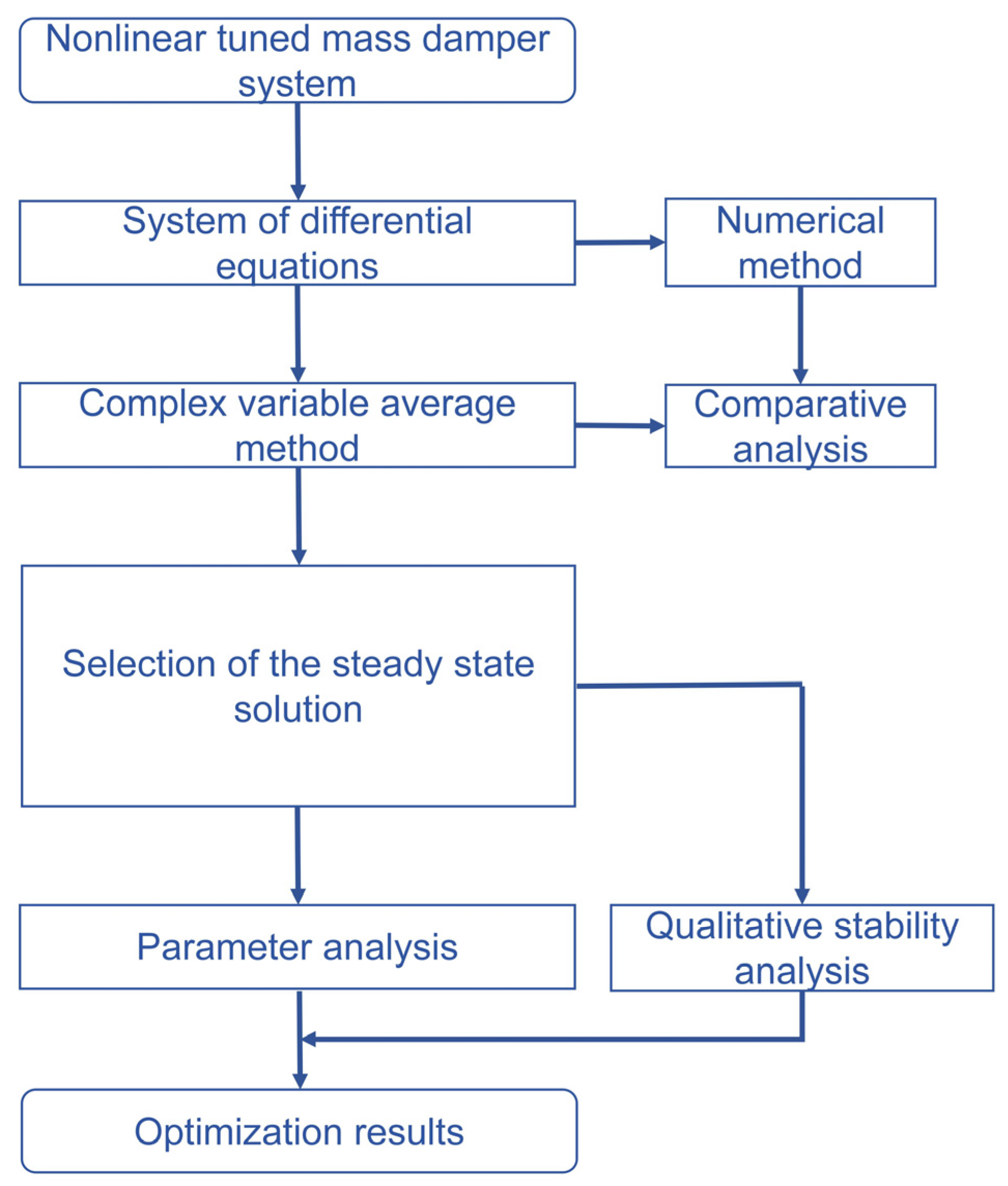
2. Theoretical Analysis of Nonlinear Tuned Mass Damper Systems

2.1. Research Methodology and Analytical Path

In this paper, the complex variable averaging method [23] is chosen to solve the system equations. Both the complex variable averaging method and the averaging method deal with the system equations in the form of setting up solutions. Unlike the averaging method, the complex variable averaging method is more convenient to solve by setting the solution in the form of complex numbers.

In the equation, the oscillations at each coordinate are assumed to be harmonics of the complex form that are of the same frequency as the excitation $F\left(t\right)$:

$$x_j(t)=\frac{A_j}{2i\omega }{e}^{i\omega t}+cc,$$

(1)

where $x_j\left(t\right)$ is a component of the state-space vector $x$, $\mathsf{\omega }$ is the frequency of the external excitation force $F\left(t\right)$, $A_j$ is a complex variable combining amplitude and phase, and $cc$ is the conjugate complex number of the previous term.

The expression for ${\dot{x}}_j\left(t\right)$ is obtained by taking the derivative of $x_j\left(t\right)$:

$${\dot{x}}_j(t)=\frac{A_j}{2}{e}^{i\omega t}+cc$$

(2)

The derivative of ${\dot{x}}_j\left(t\right)$ is then taken to obtain an expression for ${\ddot{x}}_j\left(t\right)$:

$${\ddot{x}}_j(t)={\dot{A}}_j{e}^{i\omega t}+\frac{1}{2}i\omega A_j{e}^{i\omega t}+cc$$

(3)

By substituting the expressions for $x_j\left(t\right)$, ${\dot{x}}_j\left(t\right)$, and ${\ddot{x}}_j\left(t\right)$ into the equations of the system, one is able to obtain a system of nonlinear differential equations. The results of the complex variable averaging method are the same as those of the averaging method, but its complex form is shorter than the trigonometric function form and is simpler to analyze.

The analytical path studied in this paper is shown in Figure 1.

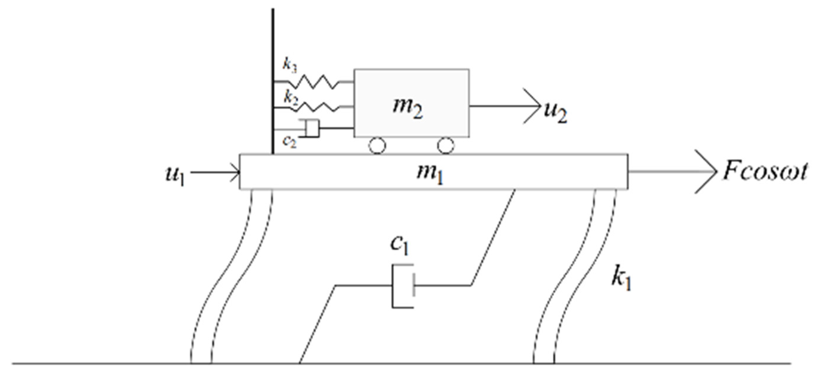
2.2. Balance Equation of the System

A dynamical system consisting of a tuned mass damper and a single-degree-of-freedom main structure excited by a simple harmonic load is shown in Figure 2. A harmonic excitation with amplitude $F$ and frequency $\omega$ is applied to the main structure. The masses of the main structure and the TMD are $m_1$ and $m_2$, respectively. $k_1$ and $k_2$ are the linear stiffnesses of the springs. $k_3$ is the nonlinear stiffness generated by the springs of the TMD during its usage. $c_1$ and $c_2$ are the linear damping. $u_1$ is the displacement of the main structure and $u_2$ is the displacement of the TMD.

The equation of motion of the system is obtained according to Newton’s second law:

$$m_1{\ddot{u}}_1+c_1{\dot{u}}_1+k_1{u}_1+m_2{\ddot{u}}_2=F\cos \omega t$$

(4)

$$m_2{\ddot{u}}_2+c_2\left({\dot{u}}_2-{\dot{u}}_1\right)+k_2\left(u_2-u_1\right)+k_3{\left(u_2-u_1\right)}^3=0$$

(5)

To simplify Equations (4) and (5), set the following parameters to perform a dimensionless transformation of the equation:

$$\begin{array}{c}\frac{F}{L{k}_1}=\epsilon f,\frac{m_2}{m_1}=\epsilon {\alpha }_1,\frac{u_1}{L}=x,\frac{u_1-u_2}{L}=y,\frac{k_1}{m_1}={\omega }_1^2,\frac{k_2}{m_2}={\omega }_2^2,{\omega }_{1}t=\tau \\ \frac{\omega }{{\omega }_1}=\mathsf{\Omega },\frac{c_1}{m_1{\omega }_1}=\epsilon {\lambda }_1,\frac{c_2}{m_2{\omega }_1}={\lambda }_2,\frac{{\omega }_2}{{\omega }_1}={\mathsf{\Omega }}_2,\frac{k_3{L}^2}{k_2}={\alpha }_2\end{array}$$

Among them, $k_1/m_1={\omega }_1^2$ is used to denote the frequency of the main structure. The ratio of the TMD to the mass of the main structure is set to $\epsilon {\alpha }_1$. $\epsilon$ is a small dimensionless parameter, which is set for the use of the method of complex variable averaging. The dimensionless coefficient $\tau ={\omega }_{1}t$ is used as the new time variable. $L$ is the unit length to be used only as a dimensionless transformation. $x=u_1/L$ is the displacement of the main structure and $y=(u_1-u_2)/L$ is the relative displacement of the main structure and the TMD. The dimensionless damping coefficient $\epsilon {\lambda }_1$ is used to replace the damping coefficient $c_1$, and the dimensionless damping coefficient ${\lambda }_2$ is used to replace the damping coefficient $c_2$. The dimensionless coefficient ${\alpha }_2$ denotes the nonlinear coefficient of the NTMD. The ratio of the frequency of the TMD to that of the main structure is replaced by the dimensionless coefficient ${\mathsf{\Omega }}_2$, and the ratio of the excitation frequency to the frequency of the main structure is replaced by the dimensionless coefficient $\mathsf{\Omega }$, while the excitation force will be denoted using $\epsilon f$.

Substituting the above dimensionless coefficients into Equations (4) and (5), the dimensionless form of the system equation of motion can be found:

$$\left(1+\epsilon {\alpha }_1\right)\ddot{x}+\epsilon {\lambda }_1\dot{x}+x-\epsilon {\alpha }_1\ddot{y}=\epsilon f\cos \mathsf{\Omega }t$$

(6)

$$\ddot{y}-\ddot{x}+{\lambda }_2\dot{y}+{\mathsf{\Omega }}_2^{2}y+{\alpha }_2{\mathsf{\Omega }}_2^2{y}^3=0$$

(7)

Decoupling Equations (6) and (7) yields

$$\frac{\ddot{x}}{{\alpha }_1}+\epsilon {\lambda }_2\dot{y}+\epsilon {\mathsf{\Omega }}_2^{2}y+\frac{\epsilon {\lambda }_1}{{\alpha }_1}\dot{x}+\frac{1}{{\alpha }_1}x+\frac{\epsilon {\alpha }_2{\mathsf{\Omega }}_2^2}{{\alpha }_1}{y}^3=\frac{\epsilon f}{{\alpha }_1}\cos \mathsf{\Omega }t$$

(8)

$$\frac{1}{1+\epsilon {\alpha }_1}\ddot{y}+{\alpha }_1{\lambda }_2\dot{y}+{\mathsf{\Omega }}_2^{2}y+{\alpha }_1{\alpha }_2{\mathsf{\Omega }}_2^2{y}^3+\frac{\epsilon {\lambda }_1\dot{x}}{1+\epsilon {\alpha }_1}+\frac{x}{1+\epsilon {\alpha }_1}=\frac{\epsilon f\cos \mathsf{\Omega }t}{1+\epsilon {\alpha }_1}$$

(9)

By applying the Taylor series, the Equations (8) and (9) are expanded on the small parameter ε, that is, $f\left(0+\epsilon \right)=f\left(0\right)+f^{\prime }\left(\epsilon \right)$:

$$\ddot{x}+x+\epsilon \left({\alpha }_1{\lambda }_2\dot{y}+{\alpha }_1{\mathsf{\Omega }}_2^{2}y+{\alpha }_1{\alpha }_2{\mathsf{\Omega }}_2^2{y}^3+{\lambda }_1\dot{x}-f\cos \mathsf{\Omega }t\right)=0$$

(10)

$$\begin{array}{l}\ddot{y}+y+{\lambda }_2\dot{y}+{\mathsf{\Omega }}_2^{2}y+{\alpha }_2{\mathsf{\Omega }}_2^2{y}^3+(x-y)\\ +\epsilon \left(-{\alpha }_1\ddot{y}+{\lambda }_2\dot{y}+{\lambda }_1\dot{x}-x+{\alpha }_2{x}^3-f\cos \mathsf{\Omega }t\right)=0\end{array}$$

(11)

Equation (11) can be simplified to the following form by omitting the first-order small quantity:

$$\ddot{y}+y+{\lambda }_2\dot{y}+{\mathsf{\Omega }}_2^{2}y+{\alpha }_2{\mathsf{\Omega }}_2^2{y}^3+(x-y)=0$$

(12)

Analyzing the above treatment, it can be found that for any similar system, the controlled structure frequency can be transformed to 1 by a dimensionless transformation. Thus, our study of the controlled structure with a frequency of 1 is equivalent to the study of all similar structures.

2.3. Complex Variable Averaging Method for Solving

According to the complex variable averaging method proposed by Manevitch in 1999 [23], the solution is set to a complex variable form that is the same as the excitation frequency. $x$ and $y$ can be set to the form of Equation (13), where $A_1$ is the complex variable expression for the amplitude and phase of $x$, $A_2$ is the complex variable expression for the amplitude and phase of $y$, and $cc$ is the conjugate complex number in the first half of the equation:

$$\{\begin{array}{l}x=\frac{1}{2i\mathsf{\Omega }}{A}_1{e}^{i\mathsf{\Omega }t}+cc\\ y=\frac{1}{2i\mathsf{\Omega }}{A}_2{e}^{i\mathsf{\Omega }t}+cc\end{array}$$

(13)

The expressions for $\dot{x}$ and $\dot{y}$ are obtained by taking the derivative of Equation (13):

$$\{\begin{array}{l}\dot{x}=\frac{1}{2}{A}_1{e}^{i\mathsf{\Omega }t}+cc\\ \dot{y}=\frac{1}{2}{A}_2{e}^{i\mathsf{\Omega }t}+cc\end{array}$$

(14)

Taking the derivative of Equation (14) obtains the expressions for $\ddot{x}$ and $\ddot{y}$:

$$\{\begin{array}{l}\ddot{x}={\dot{A}}_1{e}^{i\mathsf{\Omega }t}+\frac{1}{2}i\mathsf{\Omega }{A}_1{e}^{i\mathsf{\Omega }t}+cc\\ \ddot{y}={\dot{A}}_2{e}^{i\mathsf{\Omega }t}+\frac{1}{2}i\mathsf{\Omega }{A}_2{e}^{i\mathsf{\Omega }t}+cc\end{array}$$

(15)

It is worth mentioning that, for consistency of form, the $cc$ terms of Equations (14) and (15) include all higher-order and conjugate complex terms except the $e^{i\mathsf{\Omega }t}$ term, since only the $e^{i\mathsf{\Omega }t}$ term and its coefficients will be of concern in the subsequent study. The expressions of $x,y,\dot{x},\dot{y},\ddot{x},\ddot{y}$ are substituted into Equations (10) and (12). As this article focuses solely on the 1:1 resonance case, Ω is set to 1, and only the $e^{it}$ term is retained. From their triangular form, it can be seen that this exponential term is equivalent to the resonance harmonic quantity with a frequency of 1, which is a long-term term in perturbation methods and needs its preceding coefficients to be zero to obtain the constraint equation. The following Equations (16) and (17) can be obtained:

$$2{\dot{A}}_1+\epsilon \left({\alpha }_1{\lambda }_2{A}_2-i{\alpha }_1{\mathsf{\Omega }}_2^2{A}_2-\frac{3i{\alpha }_1{\alpha }_2{\mathsf{\Omega }}_2^2}{4}{\left|A_2\right|}^2{A}_2+{\lambda }_1{A}_1-f\right)=0$$

(16)

$$2{\dot{A}}_2+{\lambda }_2{A}_2-i{\mathsf{\Omega }}_2^2{A}_2-\frac{3i{\alpha }_2{\mathsf{\Omega }}_2^2}{4}{\left|A_2\right|}^2{A}_2-i{A}_1+i{A}_2=0$$

(17)

If the steady-state response of the structure is studied, let ${\dot{A}}_1={\dot{A}}_2=0$, and expand the expressions of $A_1$ and $A_2$ into complex forms:

$$\{\begin{array}{l}{A}_1=a_1\left(\cos b_1+i\sin b_1\right)\\ A_2=a_2\left(\cos b_2+i\sin b_2\right)\end{array}$$

(18)

where $a_1$ and $a_2$ are the steady-state amplitudes and $b_1$ and $b_2$ are the steady-state phases. Substituting Equation (18) into Equations (16) and (17) and separating the real and imaginary parts gives Equation (19):

$$\{\begin{array}{l}{a}_1\cos \left(b_1-b_2\right)=-{\mathsf{\Omega }}_2^2{a}_2-\frac{3}{4}{\alpha }_2{\mathsf{\Omega }}_2^2{a}_2^3+a_2\\ a_1\sin \left(b_1-b_2\right)=-{\lambda }_2{a}_2\\ -{\lambda }_1{\mathsf{\Omega }}_2^2{a}_2-{\lambda }_1\frac{3}{4}{\alpha }_2{\mathsf{\Omega }}_2^2{a}_2^3+{\lambda }_1{a}_2+{\alpha }_1{\lambda }_2{a}_2=f\cos b\\ {\lambda }_1{\lambda }_2{a}_2+{\alpha }_1{\mathsf{\Omega }}_2^2{a}_2+\frac{3}{4}{\alpha }_1{\alpha }_2{\mathsf{\Omega }}_2^2{a}_2^3=f\sin b\end{array}$$

(19)

3. Nonlinear Analysis

3.1. Analysis of Multivalued Phenomena in the System

Equation (19) shows the modulation–demodulation equation obtained by solving Equations (4) and (5) using the complex variable averaging method, and the steady-state response of the system can be quickly solved by programming this modulation–demodulation equation. Compared with the Eulerian and Runge–Kutta methods, which directly solve the system of differential equations and take a long time to converge to the steady-state response, the approximate analysis method is able to obtain the steady-state response very quickly.

The mass, stiffness, and damping coefficients of the main structure are set as

$$m_1=1\mathrm{kg}; k=1 \mathrm{N}/\mathrm{m}; c_1=0.1\mathrm{Ns}/\mathrm{m}$$

Other parameters are set as

$$m_2=0.02 \mathrm{kg}; c_2=0.0033 \mathrm{Ns}/\mathrm{m}; k_1=0.0187 \mathrm{N}/\mathrm{m}; k_2=0 \mathrm{N}/\mathrm{m}$$

The corresponding dimensionless parameter is

$$\epsilon =0.02; {\alpha }_1=1; {\alpha }_2=0.2; f=15; {\lambda }_1=5; {\lambda }_2=0.165$$

With the aforementioned parameter settings, the frequency ratio–amplitude curves can be seen in Figure 3. It is worth mentioning that the units in Equations (4) and (5) have been removed by dimensionless transformation. As a result, there are no unit symbols on the axes in Figure 3 and subsequent figures. Upon observing Figure 3, it becomes evident that the figure illustrates the presence of multivalued solutions in certain regions, with the solutions in these corresponding areas being unstable (indicated by the dotted portion of the red curve). Using the Runge–Kutta method, calculations were performed with the initial displacements of the primary structure set to 0 and 5, respectively, while keeping other initial conditions at 0. As depicted in Figure 3, when the initial displacement of the primary structure is set to 0 (blue curved portion), the steady-state amplitude occurs in the upper branch within the unstable frequency band of the tuned mass damper and transitions to the lower branch when the frequency surpasses the unstable region. Conversely, when the initial displacement of the primary structure is set to 5 (green curve part), the steady-state amplitude within the unstable frequency band appears in the lower branch of the graph and transitions to the upper branch as the frequency decreases beyond the unstable frequency band of the tuned mass damper. In summary, large initial displacements result in small amplitudes in the main structure, whereas small initial displacements lead to large amplitudes in the main structure. Additionally, these amplitudes may experience jumps as the TMD frequency changes. The occurrence of such a jumping phenomenon poses significant risks in engineering practice and should be avoided whenever possible. Therefore, the setting of the initial displacement is of some significance in reducing the steady-state amplitude of the structure.

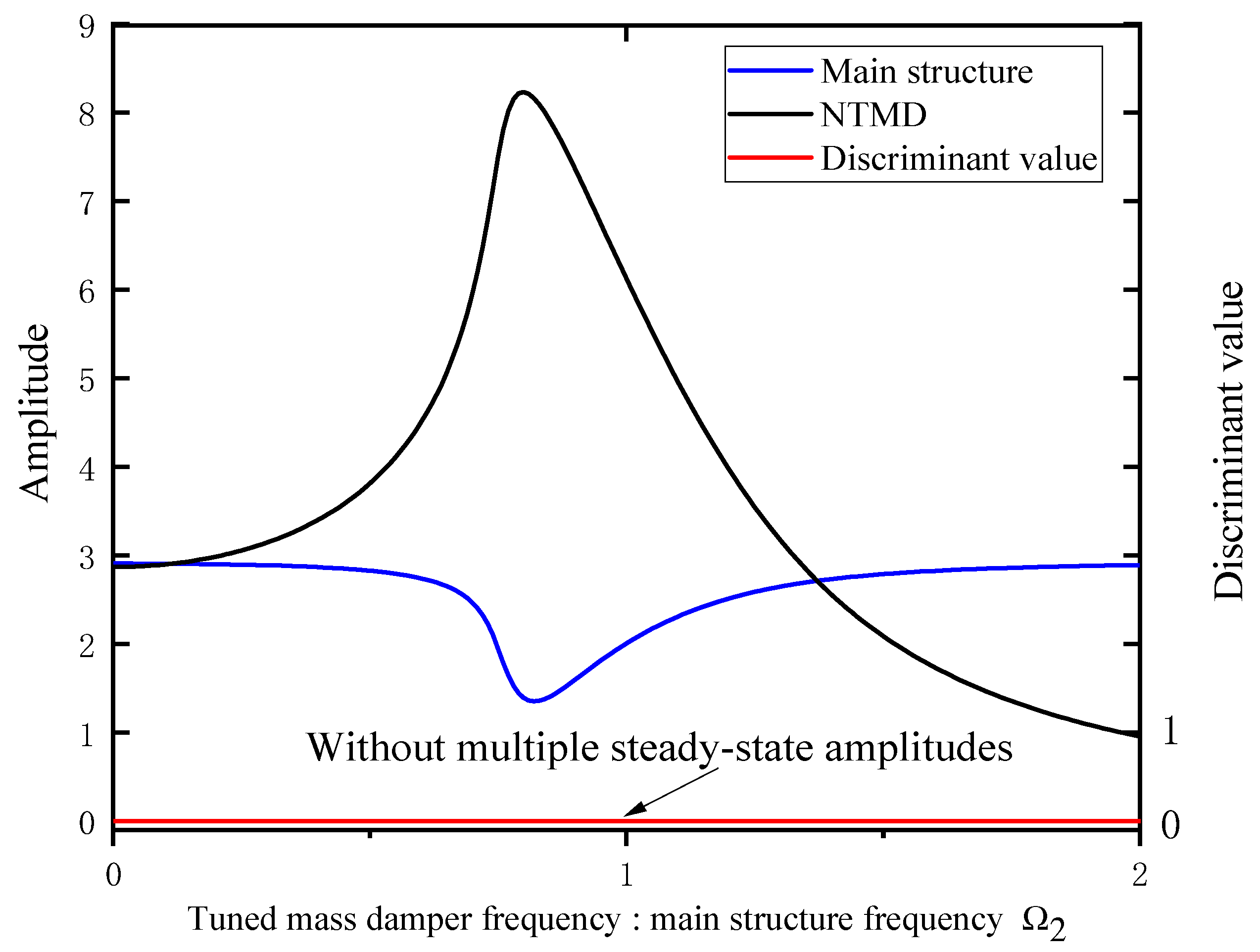
3.2. Discriminant of Jump Phenomenon

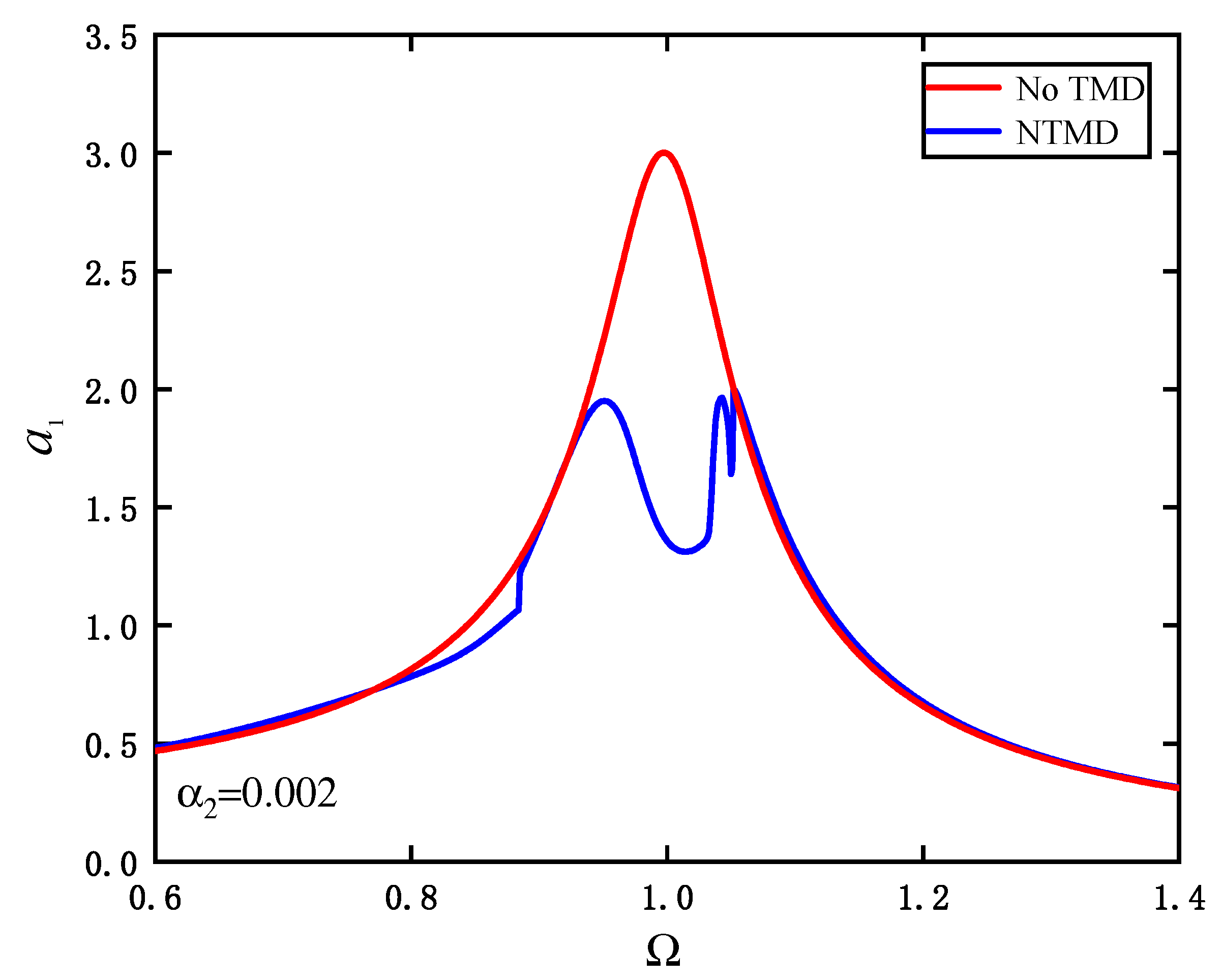
In many practical structural applications, the complexity of the response inevitably increases due to the emergence of nonlinear properties. To preemptively determine whether the structure will experience the jump phenomenon during the design stage, it is essential to discriminate in advance. Employing the modulation–demodulation Equation (19) concerning the relative displacement $a_2$, trigonometric operations are utilized to derive the expression Equation (20) for $a_1$ in terms of $a_2$, as well as the nonlinear Equation (21), solely pertaining to $a_2$:

$$a_1^2={\left(-{\mathsf{\Omega }}_2^2{a}_2-\frac{3}{4}{\alpha }_2{\mathsf{\Omega }}_2^2{a}_2^3+a_2\right)}^2+{\lambda }_2^2{a}_2^2$$

(20)

$$\begin{array}{l}{a}_2^2{\left(-{\lambda }_1{\mathsf{\Omega }}_2^2+{\lambda }_1+{\alpha }_1{\lambda }_2-\frac{3}{4}{\lambda }_1{\alpha }_2{\mathsf{\Omega }}_2^2{a}_2^2\right)}^2\\ +a_2^2{\left({\lambda }_1{\lambda }_2+{\alpha }_1{\mathsf{\Omega }}_2^2+\frac{3}{4}{\alpha }_1{\alpha }_2{\mathsf{\Omega }}_2^2{a}_2^2\right)}^2=f^2\end{array}$$

(21)

Since Equation (21) is too complicated, it is organized to obtain the sixth power of one, Equation (22), with respect to $a_2$:

$$A{a}_2^6+B{a}_2^4+C{a}_2^2+D=0,$$

(22)

where

$$\{\begin{array}{l}\mathrm{A}=\left(\frac{9{\alpha }_1^2{\alpha }_2^2{\mathsf{\Omega }}_2^4}{16}+\frac{9{\lambda }_1^2{\alpha }_2^2{\mathsf{\Omega }}_2^4}{16}\right)\\ B=3{\alpha }_1{\alpha }_2{\mathsf{\Omega }}_2^2\left({\alpha }_1{\mathsf{\Omega }}_2^2+{\lambda }_1{\lambda }_2\right)-\frac{3{\alpha }_2{\lambda }_1{\mathsf{\Omega }}_2^2\left(-{\lambda }_1{\mathsf{\Omega }}_2^2+{\lambda }_1+{\alpha }_1{\lambda }_2\right)}{2}\\ C=\left[{\left({\alpha }_1{\mathsf{\Omega }}_2^2+{\lambda }_1{\lambda }_2\right)}^2+{\left(-{\lambda }_1{\mathsf{\Omega }}_2^2+{\lambda }_1+{\alpha }_1{\lambda }_2\right)}^2\right]\\ D=-f^2\end{array}$$

(23)

Equation (22) contains only even powers and can be considered a cubic equation. In 1545, the Italian mathematician Cardano analyzed expressions of the form $J^3+PJ+Q=0$ in his work ‘Ars Magna’ [36]. In order to have the same form as the expression for the Cardano analysis, let $J=a_2^2-B/3A$, changing Equation (22) to the form of Equation (24):

$$J^3+PJ+Q=0,$$

(24)

where

$$\{\begin{array}{l}P=\frac{3AC-B^2}{3A^2}\\ Q=\frac{27A^{2}D-9ABC+2B^3}{27A^3}\end{array}$$

(25)

The authors applied Cardano’s solution to this equation. After presenting a formula for solving cubic equations, Cardano then analyzed the solutions of the equations. Cardano [36] proposed a discriminant formula to discriminate the existence of multiple real-number solutions to the cubic equation, which is exactly what is needed in this paper. The discriminant formula proposed by Cardano is as follows:

$$\frac{Q^2}{4}+\frac{P^3}{27}>0$$

(26)

If the Discriminant (26) holds, the nonlinear mass damping system is in a stable state under such parameters. If ${\mathrm{Q}}^2/4+P^3/27<0$, then there are multiple real solutions at that point. If ${\mathrm{Q}}^2/4+P^3/27=0$ and $P\ne 0$, then there is a double solution at this point, which is in a critical jump state, also known as a bifurcation point. If ${\mathrm{Q}}^2/4+P^3/27=0$, and $P=0$, then there is a single value at that point, which is the inflection point. Equation (26) can omit some positive terms, then it can be reduced as follows:

$$4{\left(3AC-B^2\right)}^3+\left(27A^{2}D-9ABC+2B^3\right)>0$$

(27)

At this point, the nonlinear tuned mass damper system is in a stable state. If there are multiple real-number solutions at this point, then the nonlinear tuned mass damper system is in an unstable state.

The correctness of the discriminant requires verification. Figure 4 displays the corresponding frequency ratio–amplitude curves and frequency ratio–discriminant plots when the nonlinear coefficient ${\mathsf{\alpha }}_2=0.01$. The same parameters are selected and substituted into the discriminant Equation (27) for assessment, and the corresponding discriminant rule is established as follows: if the condition in Equation (27) is met, indicating that the nonlinear tuned mass damper system is in a stable state, the discriminant value for that point is set to 0; if the condition in Equation (27) is not met, signifying instability in the nonlinear tuned mass damper system, the discriminant value for that point is set to 1. Following the established discriminant rule, the discriminant values corresponding to the frequency ratios depicted on the right vertical axis of Figure 4 can be determined. It is evident from the amplitude curves of the primary structure and NTMD in Figure 4 that there are no multivalued solutions for the structure with this parameter setting. All the frequency ratios in Figure 4 correspond to discriminant values of 0. As per the established rules, it can be concluded that the system does not exhibit multivalued solutions under the current parameter setting, consistent with what is indicated by the amplitudes of the primary structure and the NTMD.

No multivalued phenomena are observed in the system with ${\mathsf{\alpha }}_2=0.01$, and the same result is obtained for the discriminant. When the nonlinearity coefficient ${\mathsf{\alpha }}_2$ is set to 0.1 while keeping the remaining parameters unchanged, the corresponding frequency ratio–amplitude curves and frequency ratio–discriminant plots are depicted in Figure 5. Upon examination of Figure 5, the blue curve represents the amplitude curve of the NTMD, while the black curve signifies the amplitude curve of the main structure. An instability phenomenon is clearly evident in the graph (as indicated by the dashed segments of the blue and black curves), suggesting a potential occurrence of the jump phenomenon within the system. The corresponding discriminant value for this region is 1. Thus, the discriminant effectively identifies the presence of multivalued solutions in the system. From the unstable section in Figure 5, we can infer the relationship between the main structure and the NTMD amplitude: the high branch of the main structure’s amplitude curve corresponds to the low branch of the NTMD amplitude curve, and the low branch of the main structure’s amplitude curve aligns with the high branch of the NTMD amplitude curve. Consequently, the validity of the discriminant is substantiated.

Table 1. Jump critical frequency (comparison between numerical and analytical methods).

${\mathit{\alpha }}_2$	Critical Frequency	Numerical Method	Analytical Method
0.1	the left	0.391	0.388
0.1	the right	0.413	0.416
0.2	the left	0.289	0.287
0.2	the right	0.320	0.323
0.3	the left	0.239	0.238
0.3	the right	0.272	0.274
0.4	the left	0.210	0.208
0.4	the right	0.241	0.242
0.5	the left	0.188	0.187
0.5	the right	0.218	0.220

displays the critical frequency of the jumping phenomenon obtained using both numerical and analytical methods through the discriminant, considering different values of the nonlinear coefficient (${\mathsf{\alpha }}_2=0.1, 0.2, 0.3, 0.4, 0.5$). Upon reviewing the table data, it becomes evident that the results for the jump critical frequency obtained through numerical and analytical methods closely align, which validates the high accuracy of the approximate analytical method. Additionally, as the nonlinear coefficient increases, the instability interval for structures exhibiting the jump phenomenon gradually expands, while the value of the jump critical frequency gradually decreases.

3.3. Jump Research

The previous section analyzed the case where the discriminant of the jump phenomenon is not zero, and the discriminant can be used to determine whether the structure shows a jump phenomenon. Now, we study the parameters at the critical point and consider the case where the system parameters satisfy those shown in Equation (28):

$$4{\left(3AC-B^2\right)}^3+\left(27A^{2}D-9ABC+2B^3\right)=0$$

(28)

All parameters are held constant, with the exception of setting the damping ratio ${\lambda }_2$ to 0.1. Using the approximate analytical solution method, a curve illustrating the relationship between frequency ratio and nonlinear coefficient is obtained. This curve takes on the shape of a knife edge, featuring an inflection point on the right side of the graph, as depicted in Figure 6. Upon closer examination of the graph, vertical lines are added at the position where ${\mathsf{\Omega }}_2=0.4$, revealing three distinct special value points labeled as E, F, and G. Additionally, on the right side of the curve, an inflection point labeled as H is identified, yielding a total of four special points. Point E represents the larger nonlinear coefficient corresponding to time, point F represents the smaller nonlinear coefficient corresponding to time, point G represents the nonlinear coefficient in the middle region, and point H represents the frequency ratio and nonlinear coefficient of the inflection point in the graph. We studied the effect of changes in nonlinear coefficients on the steady-state amplitude of the primary structure under the coefficients corresponding to special value points E and F, and analyzed the meaning expressed by the frequency ratio–amplitude plots corresponding to special value points G and H.

As shown in Figure 7a, when ${\mathsf{\Omega }}_2=0.4$ and ${\alpha }_2=0.098$, the amplitude of the main structure obtained for the frequency ratio is in the low branch of the curve, at the critical point of the jump of the multivalued solution. Any slight change in the system parameters at this time may lead to the appearance of the multivalued phenomenon. An increase in the nonlinear coefficient will cause a curve change. When the nonlinear coefficient ${\alpha }_2=0.15$, the frequency ratio–main structure amplitude curve is shifted to the left. At this point, the steady-state amplitude of the main structure corresponding to ${\mathsf{\Omega }}_2=0.4$ stabilizes in the lower branch of the curve and only single-valued solutions appear. Therefore, for the nonlinear coefficients corresponding to the point E for different frequency ratios, as well as the region where the nonlinear coefficients increase, the main structure amplitude is smaller and the structure is in a steady state.

As shown in Figure 7b, when ${\mathsf{\Omega }}_2=0.4$ and ${\alpha }_2=0.0636$, the amplitude of the main structure corresponding to the frequency ratio appears in the high branch of the curve, which is at the critical point of the jump of the multivalued solution. At this time, any slight change in the system parameters may lead to the appearance of the multivalued phenomenon. A decrease in the nonlinear coefficient will cause a curve change. When the nonlinear coefficient ${\alpha }_2=0.05$, the frequency ratio–main structure amplitude curve is shifted to the right, and at this time, the steady-state amplitude of the main structure corresponding to ${\mathsf{\Omega }}_2=0.4$ is stabilized at the high branch of the curve and only single-valued solutions appear. Therefore, for the nonlinear coefficients corresponding to the points F for different frequency ratios, as well as the regions where the nonlinear coefficients decrease, the amplitude of the main structure is larger and the structure is in a stable state.

As shown in Figure 8a, when ${\mathsf{\Omega }}_2=0.4$ and $0.064<{\alpha }_2<0.098$, the frequency ratio corresponds to the main structure amplitude, which appears both in the high and low branches of the curve. The region where point G is located is between points E and F and the nonlinear coefficients obtained in this region correspond to the nonlinear coefficients obtained when point E is decreased and point F is increased. Therefore, in this region, the system inevitably generates multivalued solutions, and the main structure amplitude varies with the parameters and is very unstable.

As shown in Figure 8b, when ${\mathsf{\Omega }}_2=0.674$ and ${\alpha }_2=0.013$, the frequency ratio corresponding to the amplitude of the main structure is in a stable critical state, and neither the change of the frequency ratio nor the nonlinear coefficients lead to the appearance of multivalued phenomena. When the frequency ratio increases or the nonlinear coefficient increases, the main structure amplitude can be stabilized in the lower branch of the curve and only single-valued solutions appear.

From the four special value points E, F, G, and H, the corresponding time history diagrams of the main structure’s displacement can be obtained, as shown in Figure 9a, Figure 9b, Figure 10a, and Figure 10b, respectively. The displacement time history diagrams obtained from point E reveal that the main structure’s displacement is small during the steady-state phase. Conversely, the displacement time history diagram obtained from point F shows that the main structure’s displacement during the steady-state phase is larger. An observation of the displacement time history diagrams obtained at point G indicates that the magnitude of the main structure’s displacement during the steady-state phase varies with the initial displacement conditions. Point H is at a critical point, and, therefore, its displacement time history diagrams show that the main structure’s displacement constantly oscillates between large and small.

As shown in Figure 11, the four special value points corresponding to Figure 6 divide the graph into four distinct areas from left to right: the high-branch single-value response area, the multivalue response area, the low-branch single-value response area, and the single-value response area. In the high-branch single-value response area, the system obtained by design is stable, but the steady-state amplitude of the main structure is large. The vibration reduction effect of the NTMD is poor in this area. Within the multivalued response area, the system is unstable, inevitably leading to a multivalued solution, which is very unfavorable for the structure. In the low-branch single-value response area, the system obtained by design remains stable, and the steady-state amplitude of the main structure is lower. In this area, the NTMD is highly effective in reducing vibration. In the single-value response area, both small and large amplitudes may occur.

In summary, by selecting the parameters in the single-valued solution areas and the low-branch single-valued solution areas, the NTMD can achieve a better vibration reduction effect, and at the same time, it can avoid the occurrence of multivalued phenomena. In the low-branch single-value solution area, the closer the parameters are to the curve position, the better the NTMD vibration reduction effect obtained. However, it should not be too close to the curve to prevent subtle changes in the parameters due to changes in external factors. This may lead to parameter changes in the multivalued solution area, in which case the stability of the system cannot be guaranteed and the vibration reduction effect will be greatly reduced.

Based on the previous analysis, we set the parameters ${\mathsf{\Omega }}_2=0.715$ and ${\alpha }_2=0.002$, while keeping the rest of the parameters unchanged. These parameters are within the area of the single-valued solution. The amplitude–frequency response curve of the main structure is shown in Figure 12. As seen in the figure, the main structure controlled by the NTMD exhibits better control performance across all frequency bands and effectively reduces the amplitude at the 1:1 resonance. These results demonstrate that by selecting parameters within the single-valued solution area, the parametric design of the NTMD yields better control outcomes at different external excitation frequencies.

4. Conclusions

In this paper, a linear main structure subjected to the action of harmonic excitation and controlled by an NTMD is investigated. The modulation–demodulation equations for the steady-state amplitude of the system are obtained, and the jump phenomenon discriminant for the amplitude of the structure is obtained by means of the Cardano’s formula and the cubic discriminant. This discriminant is utilized to improve the design parameters of the NTMD, enhancing its control performance while avoiding the jump phenomenon. The main focus of this paper can be divided into three parts:

• The modulation–demodulation equations for the steady-state amplitude of the system are obtained using the complex variable averaging method, taking into account the nonlinear characteristics of the TMD generated in the vibration process. The accuracy of the modulation–demodulation equations is verified by numerical methods.
• The possible jump phenomenon of the main structure is analyzed. The discriminant of the jump phenomenon is obtained by processing the modulation–demodulation equations using Cardano’s formula and the discriminant of the cubic equation. The validity of the discriminant is confirmed by the frequency–amplitude curve. The results show that the discriminant of the jump phenomenon can accurately determine whether there is a possibility of jump occurrence in the nonlinearly tuned mass damper system.
• The effect of variations in frequency ratios and nonlinear coefficients on the steady-state amplitude of the structure is investigated using the discriminant of the jump phenomenon. By analyzing the steady-state amplitudes of the system corresponding to different parameter cases, four different response areas are obtained. The results show that selecting parameters in the single-value solution area and the low-branch single-valued solution area can help the structure avoid the jump phenomenon, ensure its stability, and improve the vibration reduction effect of NTMD.

5. Shortcomings and Prospects

The steady-state response equation obtained by the complex variable averaging method is valid for the case of resonance, but the accuracy will be greatly reduced when the excitation frequency is changed. Consequently, the results in this paper are also only for the case of resonance. In the future, researchers can verify the accuracy of these results when the excitation frequency is not equal to the main structure frequency or use other approximate analytical methods to derive the steady-state response equation and improve its accuracy.

References

1. Zamora, G.; Diego, A.; Corona, L. Impact of Tuned Mass Dampers and Electromagnetic Tuned Mass Dampers on Geometrically Nonlinear Vibrations Reduction of Planar Cable Robots. Shock Vib. 2023, 2023, 6951186. [Google Scholar]
2. Lu, Z.; Zhou, M.; Ma, N.; Du, J. Comparative Studies on Nonlinear Structures with Multiple Tuned Mass Damper and Multiple Tuned Impact Damper. Int. J. Struct. Stab. Dyn. 2023, 23, 2350158. [Google Scholar] [CrossRef]
3. Lu, Z.; Wang, Z.X.; Zhou, Y.; Lu, X.L. Nonlinear dissipative devices in structural vibration control: A review. J. Sound Vib. 2018, 423, 18–49. [Google Scholar] [CrossRef]
4. Spencer, B.F.; Nagarajaiah, S. State of the Art of Structural Control. J. Struct. Eng. 2003, 129, 845–856. [Google Scholar] [CrossRef]
5. da Costa, M.M.A.; Castello, D.A.; Magluta, C.; Roitman, N. On the optimal design and robustness of spatially distributed tuned mass dampers. Mech. Syst. Signal Process. 2021, 150, 107289. [Google Scholar] [CrossRef]
6. Lin, C.C.; Ueng, J.M.; Huang, T.C. Seismic response reduction of irregular buildings using passive tuned mass dampers. Eng. Struct. 2000, 22, 513–524. [Google Scholar] [CrossRef]
7. Hoang, N.; Fujino, Y.; Warnitchai, P. Optimal tuned mass damper for seismic applications and practical design formulas. Eng. Struct. 2008, 30, 707–715. [Google Scholar] [CrossRef]
8. Song, G.B.; Zhang, P.; Li, L.Y.; Singla, M.; Patil, D.; Li, H.N.; Mo, Y.L. Vibration Control of a Pipeline Structure Using Pounding Tuned Mass Damper. J. Eng. Mech. 2016, 142, 4016031. [Google Scholar] [CrossRef]
9. Elias, S.; Matsagar, V. Research developments in vibration control of structures using passive tuned mass dampers. Annu. Rev. Control 2017, 44, 129–156. [Google Scholar] [CrossRef]
10. Kwok, K.C.S.; Samali, B. Performance of tuned mass dampers under wind loads. Eng. Struct. 1995, 17, 655–667. [Google Scholar] [CrossRef]
11. Teng, J.; Lu, Z.X.; Xiao, Y.Q. Study on TMD contact nonlinear damped vibration control of towering structures. Vib. Shock 2009, 28, 90–97. [Google Scholar]
12. Fallahpasand, S.; Dardel, M.; Pashaei, M.H. Investigation and optimization of nonlinear pendulum vibration absorber for horizontal vibration suppression of damped system. Struct. Des. Tall Spec. Build. 2015, 24, 873–893. [Google Scholar] [CrossRef]
13. Frahm, H. Device for Damping Vibrations of Bodies. U.S. Patent No. US989958A, 18 April 1911. [Google Scholar]
14. Ormondroyd, J.; Hartog, J.P. The theory of the dynamic vibration absorber. Trans. Am. Soc. Mech. Eng. 1928, 50, 9–22. [Google Scholar]
15. Den Hartog, J.P. Mechanical Vibrations, 4th ed.; Graw-Hill: New York, NY, USA, 1956. [Google Scholar]
16. Tsai, H.C.; Lin, G.C. Optimum tuned-mass dampers for minimizing steady-state response of support-excited and damped systems. Earthq. Eng. Struct. Dyn. 1993, 22, 957–973. [Google Scholar] [CrossRef]
17. Paul, H.W.; Gary, W.C. Minimal structural response under random excitation using the vibration absorber. Earthq. Eng. Struct. Dyn. 1973, 2, 303–312. [Google Scholar]
18. Sladek, J.; Klingner, R. Effect of tuned-mass dampers on seismic response. J. Struct. Div. 1983, 109, 2004–2009. [Google Scholar] [CrossRef]
19. Villaverde, R. Reduction in seismic response with heavily-damped vibration absorbers. Earthq. Eng. Struct. Dyn. 1985, 13, 33–42. [Google Scholar] [CrossRef]
20. Roberson, R. Synthesis of a nonlinear dynamic vibration absorber. J. Frankl. Inst. 1952, 254, 205–220. [Google Scholar] [CrossRef]
21. Natsiavas, S. Steady state oscillations and stability of non-linear dynamic vibration absorbers. J. Sound Vib. 1992, 156, 227–245. [Google Scholar] [CrossRef]
22. Jiang, X.A.; McFarland, D.M.; Bergman, L.A.; Vakakis, A.F. Steady state passive nonlinear energy pumping in coupled oscillators: Theoretical and experimental results. Nonlinear Dyn. 2003, 33, 87–102. [Google Scholar] [CrossRef]
23. Manevitch, L.I.; Gourdon, E.; Lamarque, C.H. Parameters optimization for energy pumping in strongly nonhomogeneous 2 dof system. Chaos Solitons Fractals 2007, 31, 900–911. [Google Scholar] [CrossRef]
24. Gatti, G.; Kovacic, I.; Brennan, M.J. On the response of a harmonically excited two degree-of-freedom system consisting of a linear and a nonlinear quasi-zero stiffness oscillator. J. Sound Vib. 2010, 329, 1823–1835. [Google Scholar] [CrossRef]
25. Li, L.Y.; Zhang, T.J. Analytical analysis for the design of nonlinear tuned mass damper. J. Vib. Control 2020, 26, 646–658. [Google Scholar] [CrossRef]
26. Wei, Y.M.; Wei, S.; Zhang, Q.L.; Dong, X.J.; Peng, Z.K.; Zhang, W.M. Targeted energy transfer of a parallel nonlinear energy sink. Appl. Math. Mech. 2019, 40, 621–630. [Google Scholar] [CrossRef]
27. Rao, A.R.M. Nonlinear system identification using empirical slow flow model. J. Struct. Eng. 2017, 44, 1. [Google Scholar]
28. Prawin, J.; Rao, A. Nonlinear System Identification of Breathing Crack Using Empirical Slow-Flow Model. In Recent Advances in Structural Engineering, Volume 1: Select Proceedings of SEC 2016; Springer: Singapore, 2019. [Google Scholar]
29. Zhang, T.J.; Li, L.Y. Analytical analysis for optimizing mass ratio of nonlinear tuned mass dampers. Nonlinear Dyn. 2021, 106, 1955–1974. [Google Scholar] [CrossRef]
30. Li, L.Y.; Du, Y.J. Design of Nonlinear Tuned Mass Damper by Using the Harmonic Balance Method. J. Eng. Mech. 2020, 146, 04020056. [Google Scholar] [CrossRef]
31. Liu, J.F.; Yao, J.; Huang, K.; Zhang, Q.; Li, Z. Analysis of a nonlinear tuned mass damper by using the multi-scale method. J. Theor. Appl. Mech. 2022, 60, 463–477. [Google Scholar] [CrossRef]
32. Hu, Y.J.; Yao, J.; Liu, J.F.; Zhang, Q. Analysis and Design of Nonlinear Tuned Mass Damper Based on Complex Variable Averaging Method. Appl. Sci. 2023, 13, 6287. [Google Scholar] [CrossRef]
33. Su, X.Y.; Kang, H.J.; Guo, T.D. Modelling and energy transfer in the coupled nonlinear response of a 1:1 internally resonant cable system with a tuned mass damper. Mech. Syst. Signal Process. 2022, 162, 108058. [Google Scholar] [CrossRef]
34. Yao, J.; Liu, J.F.; Hu, Y.J.; Zhang, Q. Optimal Design and Analysis of Nonlinear Tuned Mass Damper System. Appl. Sci. 2023, 13, 8046. [Google Scholar] [CrossRef]
35. Chowdhury, S.; Banerjee, A.; Adhikari, S. The optimal design of dynamic systems with negative stiffness inertial amplifier tuned mass dampers. Appl. Math. Model. 2023, 114, 694–721. [Google Scholar] [CrossRef]
36. Cardano, G. Ars Magna; Dover Publications: London, UK, 1545. [Google Scholar]
Figure 1. Illustration of the analytical path.
Buildings 13 02866 g001
Figure 2. Nonlinear mass dampers and main structure dynamical system.
Buildings 13 02866 g002
Figure 3. Frequency ratio–amplitude curves obtained using the Runge–Kutta method and the complex averaging method.
Buildings 13 02866 g003
Figure 4. Frequency ratio–amplitude curves and frequency ratio–discriminant values ( α 2 = 0.01 ).
Buildings 13 02866 g004
Figure 5. Frequency ratio–amplitude curves and frequency ratio–discriminant values ( α 2 = 0.1 ).
Buildings 13 02866 g005
Figure 6. Frequency ratio–nonlinear coefficient curve ( λ 2 = 0.1 ).
Buildings 13 02866 g006
Figure 7. Frequency ratio–main structure amplitude curve corresponding to points E and F.
Buildings 13 02866 g007
Figure 8. Frequency ratio–main structure amplitude curve corresponding to points G and H.
Buildings 13 02866 g008
Figure 9. Time history diagram of displacement of main structure at points E and F.
Buildings 13 02866 g009aBuildings 13 02866 g009b
Figure 10. Time history diagram of displacement of main structure at points G and H.
Buildings 13 02866 g010aBuildings 13 02866 g010b
Figure 11. System steady-state amplitude response areas.
Buildings 13 02866 g011
Figure 12. Amplitude–frequency response curve of main structure ( Ω 2 = 0.715 , α 2 = 0.002 ).
Buildings 13 02866 g012