A Simplified Analytical Model for FRP-Strengthened Curved Brittle Substrates Using the Multi-Linear Bond-Slip Law

Abstract

The utilization of fiber-reinforced polymer (FRP) composites for building reinforcement has gained widespread acceptance. However, the bond behavior between externally applied composites and strengthened substrates, which are crucial for system efficacy, has primarily focused on flat surfaces. Yet, the challenge of curved substrates, common in masonry arches and vaults, remains less explored. This study introduces a classical analytical model addressing the bond behavior between FRP plates and curved substrates. This classical approach is structured upon a simplified model that concentrates all the non-linearities of the FRP–substrate interface. The interface is described through a universal multi-linear stress–slip relationship, with the influence of the curved substrate being considered by the normal stress that impacts the interface law. Closed-form solutions for distinct bond-slip law stages are derived and verified against the previous study. Through comparisons with existing experimental data and simulations, this approach is able to predict the maximum load, the trends of the global load-slip curves, and give insights into detailed local behavior. Additionally, the exploration of employing neural networks for determining the interface law exhibits promising outcomes.

1. Introduction

Fiber-reinforced polymer (FRP) composites have been widely utilized in building reinforcement. However, there exists a research gap concerning strengthening structures with curvature, notably in the context of arches and vaults—architectural elements frequently found in masonry structures. The efficacy of externally bonded materials in strengthening masonry arches [1] and vaults [2] lies in their ability to introduce additional tensile capacity into a system. Furthermore, some experimental studies focusing on curved elements have been conducted through laboratory tests [2,3,4] and on-site assessments [5].

The effectiveness of a reinforced system significantly depends on the bond behavior, given that the weakest point typically resides at the interface between the reinforcement and the substrate. Typically, shear tests are employed to assess this property [6,7,8,9]. When dealing with curved substrates, experimental observations have highlighted that the influence of substrate curvature, along with the positioning of the reinforcement, is substantial [10,11,12,13]. In the specific experimental study presented in [10], it was observed that the extrados strengthening configuration increased the load-bearing capacity, while intrados exhibited a reduced capacity compared to flat substrates, and higher-curvature substrates showed more pronounced deviations from flat cases. The geometric characteristics introduce more complex bonding mechanisms, such as the appearance of normal stress and peeling effects.

The common method for predicting an FRP-strengthened system’s bond behavior assumes a zero-thickness interface between the FRP composite and the substrate, thereby concentrating system non-linearities at the interface. This approach is widely used due to its simplicity and intuitiveness, especially when adopting a simple mathematical form of the bond-slip law. The interface is characterized by a stress–slip relationship, also known as the bond-slip law, often represented through multi-linear [14,15,16,17,18] or exponential functions [19,20]. The current study presents comprehensive solutions for a multi-linear interface bond-slip law, specifically a quadrilinear law. This model can effectively replicate the four key stages of the interface law: the initial elastic stage, a subsequent plateau stage, the softening stage, and a final stage representing the residual strength of the interface face. The adoption of a cohesive law featuring a plateau stage has found success in previous research [21,22], effectively reproducing the observed ductility in bond behavior during experimental tests. It is important to highlight that the quadrilinear model can be easily degraded into bi-linear or trilinear laws through parameter adjustments, enhancing the versatility of the current approach to accommodate various shapes and characteristics of cohesive laws.

In this study, the author continues to use this straightforward approach to describe the bond behavior of curved systems, wherein the influence of substrate curvature on the system is simplified as the effect of the interface normal stress on the interface law. Consequently, the interface law is adjusted during the loading based on varying degrees of interface normal stress. The authors’ previous work demonstrated the efficacy of the proposed strategy in accounting for the influence of substrate curvature [16]. It should be mentioned that mode I fracture (opening fracture) is not considered in this study. For masonry structures such as arches and vaults, substantial curvature is required to trigger mode I fracture under the external load parallel to the FRP plate axis. Such curvature is typically not encountered in these structural members. For a comprehensive understanding, refer to the work by Grande et al. [23]. The interaction between FRP plates and curved substrates is modeled by shear and normal springs. The findings reveal that none of the normal springs exceed their tensile strength, thus indicating the absence of mode I fracture.

This article is structured as follows: Section 2 outlines the governing equations for the debonding phenomenon and provides closed-form solutions. The approach’s validity is established through comparisons with both existing experimental and modeling outcomes in Section 3, demonstrating its good prediction of bond strength. Furthermore, this study compares various formulations of bond-slip laws and explores the associated modeling parameters in Section 4. Section 5 showcases the application of this model in conjunction with a neural network approach to inversely deduce the interface law from experimental global curves. A comparison of the NN approach with the traditional bond-slip law determination approach is detailed in this section. The results underscore the effectiveness of this innovative approach, presenting a promising solution for scenarios where determining the interface bond-slip law proves challenging.

2. Mathematical Model Describing the Debonding Problem

As observed in the shear tests performed on FRP-strengthened curved masonry prisms, except for the fracture of the fiber textile outside the bond area, the failure is mostly shown as either a cohesive failure involving a few millimeters of the substrate material, or the detachment of the FRP from the substrate. Considering these typical modes of failure, we lump all the non-linear behavior of the reinforced system along the interface for the simplicity of modeling. We make the following assumptions to form a 2D mathematical model, as illustrated in Figure 1: (1) It is assumed that the materials and external forces exhibit uniformity across the width of the plate. (2) The external force, denoted as F, is assumed to be applied at the end of the unbonded FRP plate, acting in a direction tangential to the longitudinal axis of the plate. (3) The model comprises three components: the FRP plate behaves as linear elastic, the rigid substrate with negligible displacement, and the zero-thickness interface follows a multi-linear bond-slip law, which will be illustrated in detail in Section 2.1.

The loading procedure will be simulated by gradually increasing the slip value assigned at the free edge of the FRP plate, which is denoted as $s_0$, and the simulation will be terminated once a sufficiently large value of $s_0$ is reached, based on experimental observations.

2.1. Bond Slip Law

In this study, a multi-linear relationship is assumed for the bond-slip law $\tau -s$, as depicted in Figure 2, in which $\tau$ represents the shear stress along the FRP–substrate interface, and $s$ denotes the relative displacement between the FRP plate and the substrate. However, given the assumption of a fixed substrate, $s$ represents the FRP’s displacement as well. The influence of the substrate curvature on the reinforced system will be simply considered through the variation in the interface shear stress with respect to the interface normal stress. More specifically, the black solid line in Figure 2 represents the bond-slip law for the flat substrate case, where the interface normal stress is equal to zero. This bond-slip law is depicted as a quadrilinear relationship, which includes an initial elastic stage terminating at $s=s_e$ when reaching $\tau ={\tau }_m$, followed by a plateau stage until $s=s_p$, then a softening stage until $s=s_s$, and a final stage that exhibits a constant residual interface stress ${\tau }_r$. These four stages are subsequently designated as ‘Stage I’ to ‘Stage IV’. Notably, this quadrilinear relationship degenerates into a classical triangular relationship when $s_e=s_p$.

To establish the interface bond-slip law for the curved case, as mentioned earlier, the experimental results indicate an increase in the load-bearing capacity in the extrados strengthening case, while a decrease is observed in the intrados case with respect to the flat substrate. Moreover, cases with higher substrate curvature demonstrated more pronounced deviations from the flat case behavior.

Accordingly, we consider an increase in the interface bond strength and ductility for the extrados case (represented by the red line in Figure 2), and a reduction for the intrados case (represented by the blue line in Figure 2). These adjustments are made based on the local interface normal stress and following the Coulomb friction law, expressed mathematically as follows:

$$\left\{\begin{array}{c}{\tau }_1\left(s\right)=K_{1}s, 0<s\le s_e^{*}\\ {\tau }_2\left(s\right)={\tau }_m^{*}, s_e^{*}<s\le s_p^{*} \\ {\tau }_3\left(s\right)=K_2(s-s_p^{*})+{\tau }_m^{*}, s_p^{*}<s\le s_s^{*} \\ {\tau }_4\left(s\right)={\tau }_r^{*}, s>s_s^{*}\end{array}\right.$$

(1)

in which $K_1$ and $K_2$ represent the stiffnesses of the elastic and softening stages, respectively. Parameters denoted with an asterisk superscript indicate the values that vary with the interfacial normal stress ${\sigma }_n$. For the extrados case:

$$\left\{\begin{array}{c}{\tau }_m^{*}={\tau }_m+{\sigma }_{n}tan\varphi \\ {\tau }_r^{*}={\tau }_r+{\sigma }_{n}tan{\varphi }_r\end{array}\right.$$

(2)

in which $\varphi$ and ${\varphi }_r$ are the interface friction angle and the residual friction angle, respectively. For the intrados case, we assume no residual strength remains along the interface due to the peeling effect undermining the bond capacity towards the total debonding of the reinforced system:

$$\left\{\begin{array}{c}{\tau }_m^{*}={\tau }_m-{\sigma }_{n}tan\varphi \\ {\tau }_r^{*}=0\end{array}\right.$$

(3)

Additionally, the limitations of the different stages also vary with ${\sigma }_n$, and for the extrados case, are expressed as:

$$\left\{\begin{array}{c}{s}_e^{*}=s_e+{\sigma }_{n}tan\varphi /K_1\\ s_p^{*}=s_p+{\sigma }_{n}tan\varphi /K_1\\ s_s^{*}=s_p^{*}-({\tau }_m^{*}-{\tau }_r^{*})/K_2\end{array}\right.$$

(4)

For the intrados case, replace the plus sign with a minus sign in front of ${\sigma }_n$ in Equation (4).

2.2. Governing Equation

Take an infinitesimal portion $dx$ of the FRP plate to analyze, see Figure 1b. The independent variable $x$ represents the position of any point along the bonded length $L$, where $0\le x\le L$ and the abscissa $x=0$ corresponds to the location of the free edge. In the Cartesian coordinate system, $x_1$ represents the direction aligned with the tangent of the substrate (and also the FRP plate), while $x_2$ indicates the direction perpendicular to the tangent.

The positive direction of the interface normal stress is defined as being away from the center of the curved substrate. For both the extrados and intrados cases, the equilibrium of the infinitesimal part along the tangential direction $x_1$ can be expressed identically as follows:

$$t_F\frac{d{\sigma }_F}{dx}=\tau (s,{\sigma }_n)$$

(5)

where $t_F$ and ${\sigma }_F$ are the thickness and tensile stress of the FRP plate along its longitudinal direction separately. For the FRP plate, we can write the constitutive law as follows:

$${{\sigma }_F=E}_F\frac{ds}{dx}$$

(6)

where $E_F$ is the elastic modulus of the FRP plate. The governing ODE can be derived by substituting Equation (6) into Equation (5):

$$\frac{d^{2}s}{{dx}^2}=\frac{\tau \left(s,{\sigma }_n\right)}{E_F{t}_F}$$

(7)

The interface normal stress ${\sigma }_n$ can be gained by the equilibrium condition along the normal direction $x_2$:

$${\sigma }_n=\frac{t_F}{R}{\sigma }_F=\frac{E_F{t}_F}{R}\frac{ds}{dx}$$

(8)

With the substitution of ${\sigma }_n$ into the bond-slip law $\tau (s,{\sigma }_n)$, the ODE of Equation (7) is a second-order, non-linear differential equation with the displacement of fiber $s$ assumed as being a dependent variable of $x$.

2.3. Closed-Form Solutions

The ODE presented in the previous section can be solved analytically with appropriate boundary conditions for each stage. However, as the loading progresses, different shear stress stages appear along the interface, and we define $x_{ep}$, $x_{ps}$, and $x_{sr}$ as representing the junction points between the elastic and plateau stages, plateau and softening stages, and softening and residual strength stages, respectively.

To identify the occurrence and range of these stages along the interface, we introduce a procedure that can be easily implemented through repeated calculations using MATLAB or Excel spreadsheet. Given that the FRP plate is always under tension and behaves elastically, the fiber displacement $s\left(x\right)$ along the bond length will monotonically increase from the free edge towards the loading edge. The occurrences of different stages are associated with $s\left(x\right)$ and will always follow the sequence from Stage I to Stage IV.

To determine the initial stage at the free edge, it is straightforward to compare the assigned displacement $s_0$ with the stage limitations ($s_e$, $s_p$, and $s_s$), since no normal stress appears at this point, and thus no shifting of the limitations due to ${\sigma }_n$. At the free edge, we always have the boundary conditions as follows:

$$\left\{\begin{array}{c}s\left(x=0\right)=s_0\\ \frac{ds}{dx}\left(x=0\right)=0\end{array}\right.$$

(9)

The solutions for the initial stage can be analytically obtained with these boundary conditions, as detailed in the following sub-sections. Subsequently, we can determine the displacement value and its first derivative at the junction point between the next stage ($x_{ep}$, $x_{ps}$, or $x_{sr}$), which will then serve as the boundary conditions for the next stage. The junction point can be determined by comparing whether $s\left(x\right)$ exceeds the corresponding stage limitation ($s_e^{*}$, $s_p^{*}$, or $s_s^{*}$) or not, while considering the influence of the normal stress at each $x$ under calculation. This calculation approach, implemented through MATLAB, is summarized in Figure 3.

2.3.1. Solutions for Stage I (Elastic Stage)

As discussed in Section 2.2, the field Equation (7) remains applicable for both the extrados and intrados cases. Within the current model, the effect of normal stress is exclusively manifested through the interface stress-slip law. Therefore, in the subsequent calculations, we will present the closed-form solutions specifically for the extrados case. For the intrados case, the solutions can be easily obtained by substituting the value of the substrate radius R with a negative value and setting the parameters ${\tau }_r$ and $tan{\varphi }_r$, which relate to the residual strength, to zero.

By substituting the bond-slip law of Stage I (see the first equation of Equation (1)), the governing equation is given as:

$$\frac{d^2{s}_1}{{dx}^2}=\frac{K_1{s}_1}{E_F{t}_F}$$

(10)

The subscript of $s_1$ denotes the solution of the ODE for the bond-slip law of Stage I. Since Stage I always starts from the free edge if it appears, with the boundary conditions at the free edge as given in Equation (9), the solution for this second-order ordinary differential equation is:

$$s_1\left(x\right)=s_0\cosh \left(\gamma x\right)$$

(11)

in which $\gamma =\sqrt{K/{(E}_F{t}_F)}$. The interfacial shear and normal stresses, as well as the fiber stress, can be further determined using the first equation of Equations (1), (6) and (8).

If $s_1\left(L\right)>s_e^{*}\left(L\right)$, the interface stress will not be maintained in Stage I for the entire bond length. The range of Stage I, $x_1\in [0,x_{ep}]$, can be determined by the condition that the displacement will not exceed the limitation $s_e^{*}$, which can be expressed as follows:

$$s_0\cosh \left(\gamma x_{ep}\right)=s_e+\frac{tan\varphi }{K_1}\frac{E_F{t}_F}{R}{s}_0\gamma \sinh \left(\gamma x_{ep}\right)$$

(12)

To determine the value of $x_{ep}$, numerical methods can be resorted to. For example, one approach is to calculate the values of $s_1\left(x\right)$ and $s_e^{*}\left(x\right)$ at different $x$, starting from 0 until the former exceeds the latter. The $x_1$ value at this point can then be considered as the estimated value of $x_{ep}$. Another option is to use the ‘fsolve’ function provided by MATLAB.

2.3.2. Solutions for Stage II (Plateau Stage)

The governing equation for Stage II can be obtained by substituting the second equation of Equation (1) into Equation (7):

$$\frac{d^2{s}_2}{{dx}^2}=\frac{{\tau }_m}{E_F{t}_F}+\frac{tan\varphi }{R}\frac{d{s}_2}{dx}$$

(13)

The general solution is given as:

$$s_2\left(x\right)=C_1+C_2{e}^{\frac{tan\varphi }{R}{x}_2}-\frac{R{\tau }_m}{E_F{t}_{F}tan\varphi }{x}_2$$

(14)

The B.C.s at the left end of the Stage II range can be utilized to determine the values of the constants $C_1$ and $C_2$. The left end can be either $x=0$ or ${x=x}_{ep}$, depending on whether Stage I fades out of the bond length ($s_0>s_e$) or not ($s_0\le s_e$).

If $s_0\le s_e$, the B.C.s for Stage II will be the compatibility conditions between Stage II and Stage I. This implies that the displacement and its first derivative calculated for Stage II should be the same as the solutions obtained by Stage I at ${x=x}_{ep}$. Therefore, we can determine $C_1$ and $C_2$ as follows:

$$\left\{\begin{array}{c}{C}_1=s_1\left(x_{ep}\right)-C_2\\ C_2=\frac{R}{tan\varphi }(\frac{d{s}_1}{dx}\left(x_{ep}\right)+\frac{R{\tau }_m}{E_F{t}_{F}tan\varphi })\end{array}\right.$$

(15)

If $s_0>s_e$, the left end will be the free edge, and thus the B.C.s are as in Equation (9). $C_1$ and $C_2$ can be determined by letting $s_1\left(x_{ep}\right)=\frac{d{s}_1}{dx}\left(x_{ep}\right)=0$ in the above equation.

When $s_2\left(L\right)>s_p^{*}\left(L\right)$, Stage III will occur along the interface as well. Similar to the approach of determining the range of Stage I, the right end of Stage II, $x_{ps}$, can be determined by comparing the displacement with the Stage II limitation $s_p^{*}$ by solving $s_2\left(x_{ps}\right)=s_p^{*}\left(x_{ps}\right)$.

2.3.3. Solutions for Stage III (Softening Stage)

The governing equation for Stage III can be obtained by substituting the third equation of Equation (1) into Equation (7):

$$\frac{d^2{s}_3}{{dx}^2}=\frac{K_2}{E_F{t}_F}{s}_3+\frac{tan\varphi (1-K_2/K_1)}{R}\frac{d{s}_3}{dx}+\frac{{\tau }_m-K_2{s}_p}{E_F{t}_F}$$

(16)

The general solution is given as:

$$s_3\left(x\right)=e^{\beta x}\left(C_{3}sin\sqrt{\alpha }x+C_{4}cos\sqrt{\alpha }x\right)+\frac{K_2{s}_p-{\tau }_m }{K_2}$$

(17)

in which $\alpha$ and $\beta$ are constants given in Equation (18). It should be noted that the general solution is presented in this form under the observation that the value of $\alpha$ is positive, in accordance with commonly adopted engineering parameters.

$$\left\{\begin{array}{c}\alpha =-{\left(\frac{tan\varphi (1-K_2/K_1) }{2R}\right)}^2-\frac{K_2}{E_F{t}_F}\\ \beta =(1-\frac{K_2}{K_1})\frac{tan\varphi }{2R}\end{array}\right.$$

(18)

The constants $C_3$ and $C_4$ need to be determined by the B.C.s at the left end of Stage III. Similar to the analysis for Stage II, the left end can be either $x=0$ or ${x=x}_{ps}$, depending on whether Stage II fades out of the bond length ($s_0>s_P$) or not ($s_0\le s_P$).

If $s_0\le s_P$, the B.C.s for Stage II are the compatibility conditions between Stage III and Stage II, and $C_3$ and $C_4$ are as follows:

$$\left\{\begin{array}{c}{C}_3=(\frac{d{s}_2}{dx}\left(x_{PS}\right)-\beta C_4)/\sqrt{\alpha }\\ C_4=s_2\left(x_{PS}\right)+({\tau }_m-K_2{s}_p)/K_2\end{array}\right.$$

(19)

If $s_0>s_P$, the left end will be the free edge, and $C_3$ and $C_4$ can be determined by letting $s_2\left(x_{ps}\right)=\frac{d{s}_2}{dx}\left(x_{ps}\right)=0$ in Equation (19).

When $s_3\left(L\right)>s_s^{*}\left(L\right)$, we need to determine the right end of Stage III, $x_{sr}$. This can be achieved by considering whether the displacement exceeds the Stage III limitation, which can be solved by setting $s_3\left(x_{sr}\right)=s_s^{*}\left(x_{sr}\right)$.

2.3.4. Solutions for Stage IV (Residual Strength Stage)

Upon observing the expressions for the bond-slip law in Stage II and Stage IV, it becomes evident that the expressions are identical, except for the distinction between ${\tau }_m$ and ${\tau }_r$, as well as $tan\varphi$ and $tan{\varphi }_r$. Consequently, the solutions for Stage IV can be readily obtained by substituting ${\tau }_m$ with ${\tau }_r$ and $tan\varphi$ with $tan{\varphi }_r$ in the solutions for Stage II, as presented in Section 2.3.2. Similarly, the B.C.s can be determined either by the conditions at the free edge or the compatibility conditions with Stage III at the junction point $x_{sr}$.

3. Validation and Comparisons with Existing Data

In this section, we will validate and compare the current approach with existing data, encompassing both experimental and modeling results. The experimental campaign by Rotunno et al. [10] provided a basis for our comparative analysis. This campaign involved shear tests on five sets of CFRP-strengthened masonry prisms, including one group with a flat substrate, two groups with a substrate radius of 1500 mm strengthened on either the extrados (CAE) or intrados (CAI), and two other groups with a substrate radius of 3000 mm strengthened on the extrados (CBE) or intrados (CBI).

This experimental setup also served as a basis for the numerical model introduced by Milani et al. [19], where the debonding problem was characterized using the same ODE as that proposed in our study. However, the bond-slip law was described using an exponential function, and the ODE was subsequently numerically solved using finite differences. The authors’ previous work [16], conducted within the same framework but employing a classical trilinear law, is also subjected to comparison.

3.1. Validating Solution Accuracy

Verification of the accuracy of the closed-form solutions can be effectively accomplished by comparing them with our previous study [16]. This earlier investigation focused on the same debonding issue in a curved substrate context and incorporated substrate curvature via interface normal stress in a classical trilinear interface law. Apart from the shape of the interface law, a significant distinction lies in the inclusion of a constant residual strength assumed for the flat and extrados cases in the current study. Another difference is that the previous study did not account for any adjustments to the stage limits based on the normal stress, allowing for a determination of the junction points between various stages using closed-form solutions.

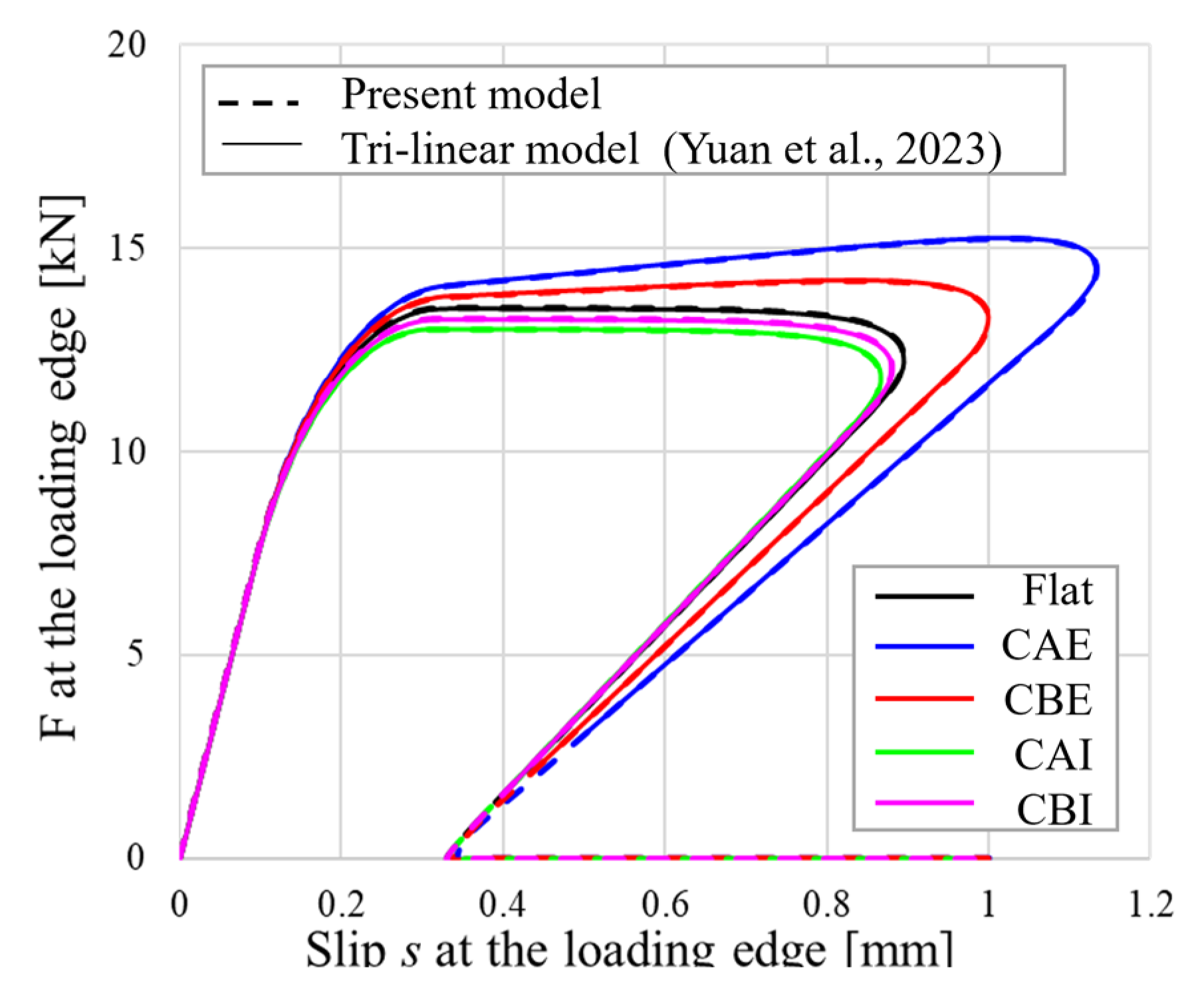
As mentioned earlier, the current model can also be adapted to a trilinear law by setting $s_p=s_e$, enabling a direct comparison between the global load-slip curves derived from previous solutions and our present solutions. As depicted in Figure 4, a high degree of alignment is evident for all the cases under investigation. The disparities between our current approach and the trilinear model employed for the validation are detailed in

Table 1. Validation of the present quadrilinear model regarding the characteristic values from global load-slip curves.

Cases	Models	Maximum Slip (mm)	Maximum Load (kN)
FLAT	Trilinear law	0.8945	13,530.69
	Quadrilinear law	0.8952 (0.72‰)	13,531.93 (0.09‰)
CAE	Trilinear law	1.1314	15,243.89
	Quadrilinear law	1.1327 (1.16‰)	15,244.11 (0.01‰)
CBE	Trilinear law	0.9999	14,208.04
	Quadrilinear law	1.0000 (0.08‰)	14,207.98 (0.004‰)
CAI	Trilinear law	0.8659	13,011.44
	Quadrilinear law	0.8662 (0.37‰)	13,011.51 (0.01‰)
CBI	Trilinear law	0.8800	13,266.33
	Quadrilinear law	0.8804 (0.51‰)	13,266.39 (0.005‰)

Note: In parentheses are the differences between the current model and the trilinear model for verification.

, with a focus on the maximum load and slip before the snapback phenomenon. Notably, the observed differences are exceedingly small. This suggests that an adjustment of the stage limits does not exert a substantial influence on the global load-slip curves. This outcome aligns with our expectations, given the negligible normal stress induced by the large substrate radius, resulting in minimal alterations to the stage limits. Modeling parameters remain detailed in

Table 2. Parameters adopted for the simulation.

Groups			CAE	CBE	CAI	CBI	Flat
Substrate	Strengthening Position		Extrados	Extrados	Intrados	Intrados	/
	Radius	R (mm)	1500	3000	−1500	−3000	${10}^8$
FRP plate	Elastic modulus	$E_F$ (MPa)	250,000
	Thickness	$t_F$ (mm)	0.165
	Width	$B_F$ (mm)	100
	Bond length	$L$ (mm)	382	354	330	330	330
Interface	Bond strength	${\tau }_m$ (N/mm2)	1.37
	Residual strength	${\tau }_r$ (N/mm2)	0.05	0.05	0	0	0.05
	Elastic limit	$s_e$ (mm)	0.07
	Plateau limit	$s_p$ (mm)	0.11
	Softening limit	$s_s\left(\mathrm{m}\mathrm{m}\right)$	0.26
	Friction angle	$\varphi$(°)	35
	Residual friction angle	${\varphi }_r$ (°)	35	35	${10}^{-8}$	${10}^{-8}$	35

, wherein a zero value of the residual strength ${\tau }_r$ is assumed to align with the previous model.

3.2. Comparisons with Existing Data

The parameters for the simulation are presented in Table 2. It should be noted that the fracture energy and the bond strength of the interface law closely resemble those utilized in [10], which were derived from strain data acquired through strain gauges placed on the external surface of a CFRP, see study [19] for further details. The interface laws employed for the flat case in the previous numerical model [19], as well as in [16], using a classical trilinear law, are depicted in Figure 5.

Worth mentioning is that a considerably larger value of the substrate radius is adopted to simulate the flat situation, while for the intrados case, to continue to utilize the solutions gained for the extrados case, the substrate radius will be set to be negative; additionally, to prevent potential issues where zero values might arise in the denominator, considerably small values are employed for ${\varphi }_r$ instead of zero.

The global load-slip curves derived from the present model are presented in Figure 6a, where distinct line types represent different groups and various colors signify different stage combinations along the bond length. Notably, an ascending part is discernible for the flat and extrados cases, while it is absent for the intrados case. This ascending part is attributed to the emergence of the residual strength stage (Stage IV), which, for intrados cases, corresponds to zero stress. The substrate curvature directly impacts the interface normal stress and, consequently, the interface stress. As a result, we can observe that the CAE case demonstrates the highest bond strength, while the CAI case exhibits the lowest.

The load-slip curves obtained using the current and existing approaches are compared in Figure 6b–f. The modeling outcomes show a good agreement, the two analytical models exhibit only slight disparities, and both display snap-back behavior, which is not present in the numerical modeling results. This difference can be attributed to the distinct loading process simulation approaches: in the analytical models, increasing slips were imposed at the free edge, whereas, in the numerical model, slip increments were applied at the loading edge, naturally precluding any reduction in the slip.

Comparing the modeling results with the experimental data, a good resemblance is evident in terms of the initial elastic behavior and bond strength. However, all these models give too brittle behavior compared to the experimental results. This might be attributed to the simplification of the modeling, such as ignoring the damage spread inside the substrate and the interlocking provided by the mortar joints, etc.

The current methodology offers a comprehensive insight into the propagation of interface slip and stresses, utilizing cases CAE and CAI as exemplars, as illustrated in Figure 7. Different lines indicate the different stages appearing along the bond length. The slip patterns clearly show the influence of each stage corresponding to their respective limitations. The distribution of interface shear stresses demonstrates a noticeable progression from the loading edge to the free edge, including the appearance of the plateau and softening stages, eventually reaching the residual strength phase. Notably, the normal stresses within the two cases exhibit opposing signs, a consequence of our negative radius assumption for the intrados case. Additionally, the normal stress consistently remains at a low level, mainly due to the substantial substrate radius.

4. Discussions Regarding the Interface Law

In a previous study based on trilinear laws [16], an extensive investigation of the impacts of the parameters embedded in the interface law was conducted. It was ascertained that the bond strength of the reinforced system mostly depended on the fracture energy of the interface, regardless of the precise configuration of the interface law, as corroborated by the findings thus far [16,17,24]. Further conclusions have been drawn, highlighting that the interface friction angle and residual friction angle exerted minimal influence on the global curves, owing to the considerably low magnitude of the interface normal stress. Therefore, within this section, our focus will center on investigating the contrasts between the current multi-linear model and the previous trilinear-law-based model, while also examining the effects of residual strength. This analysis will be undertaken while maintaining consistent values for the friction angles.

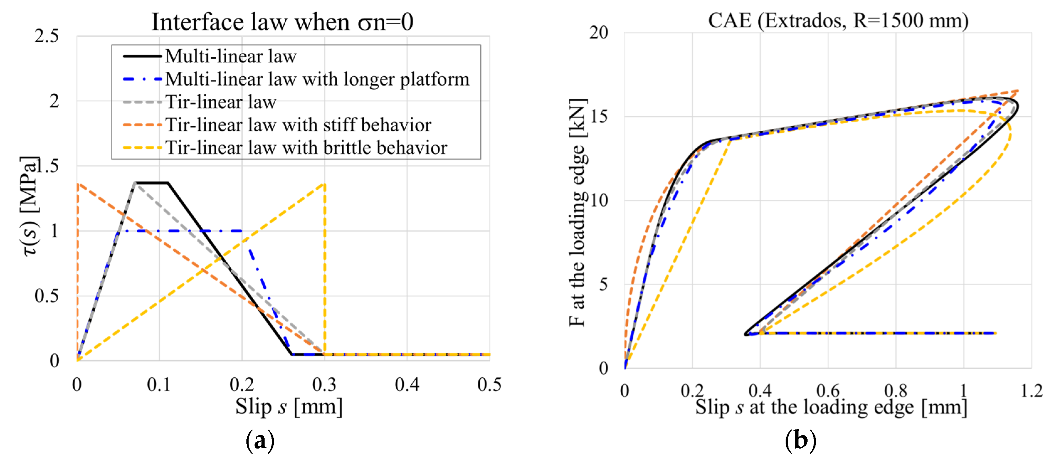
Thanks to the adaptability and robustness provided by the analytical approach, this section aims to assess various commonly employed forms of interface laws, as illustrated in Figure 8a. The comparisons encompass classic trilinear laws, trilinear laws exhibiting either rigid or brittle behavior, and quadra-linear laws with differing plateau stage durations. It should be noted that all these relationships share closely aligned fracture energy values. The global load-slip curves for case CAE are presented in Figure 8b. The differences corresponding to the elastic stiffness and beginning of the residual stage can be identified, nonetheless, due to the near-identical fracture energy values, and the results demonstrate an overall convergence.

Figure 9 illustrates the global load-slip curves obtained using different values of residual strength (${\tau }_r$) for both the CAE and CBE cases, maintaining the other parameters at the values specified in Table 2. Increased values of ${\tau }_r$ result in a more pronounced ascending part, a higher global bond strength, and a higher residual strength. Notably, in the CAE case, higher ${\tau }_r$ values contribute to a closer approximation of the global curve. However, for the CBE case, characterized by lower substrate curvature, large ${\tau }_r$ values appear to be less suitable, suggesting the feasibility of adopting distinct ${\tau }_r$ values to account for cases with varying substrate curvatures.

5. Parameters Determination via Neural Network

A proper determination of the bond-slip law is essential for replicating the observed bond behavior during shear tests. One common method for achieving this involves the placement of strain gauges along the bond length during the test [2,25,26]. By analyzing the strain data, it becomes possible to derive shear stress and slip through differentiation and integration, respectively. This direct approach offers the advantage of not necessitating prior knowledge of the mathematical form of the bond-slip law. However, despite its conceptual simplicity, experimental outcomes generally show a high discreteness. Consequently, this approach often yields bond-slip curves of irregular shapes, demanding user interpretation to choose an appropriate bond-slip law for simulation purposes, as exemplified in this study.

Another approach involves utilizing global load-slip data obtained experimentally to deduce the bond relationship in a reverse manner, which is termed ‘inverse calibration’ in some research [8,27,28]. Initially, a mathematical form for the bond-slip law needs to be assumed, then some key features (such as maximum load and fracture energy, etc.) and the global curves are derived based on this assumption. These derived features are then adjusted to closely match the experimental data, allowing for the determination of the previously undetermined bond-slip law parameters. This method proves valuable when sufficient experimental strain data are lacking.

The conventional method used for inverse calibration involves a regression analysis, and more recently, there has been a growing interest in utilizing neural networks for achieving the same purpose [14,29]. This novel approach leverages the power of neural networks to reproduce complicated data relationships and patterns. Compared to the traditional approach, wherein traditional regression techniques aim to establish a direct functional relationship between input and output variables, neural networks serve as a data-driven black box. This distinction is particularly important when dealing with complex and nonlinear systems, since neural networks excel in capturing intricate patterns and dependencies within data, enabling them to flexibly model complex relationships between input and output variables.

In order to enhance the quality of neural network predictions, the selection of training inputs and outputs requires careful consideration. Input dimensionality, denoting the number of features of global curves in this context, needs to be able to identify the most informative features and discard the less important ones, and may lead to model complexity when excessively high. While increased outputs allow for the network to make more comprehensive predictions, they might also complicate training and necessitate a larger training dataset. It can be said that the efficiency and accuracy of training and prediction largely depend on the choice of training data, which introduces risks. Inadequate or unrepresentative training data may result in a suboptimal model performance, including the risk of overfitting, ultimately leading to inaccurate predictions. Therefore, a balanced approach is imperative to optimize the neural network’s ability to make accurate predictions while mitigating the risks associated with data quality and model complexity.

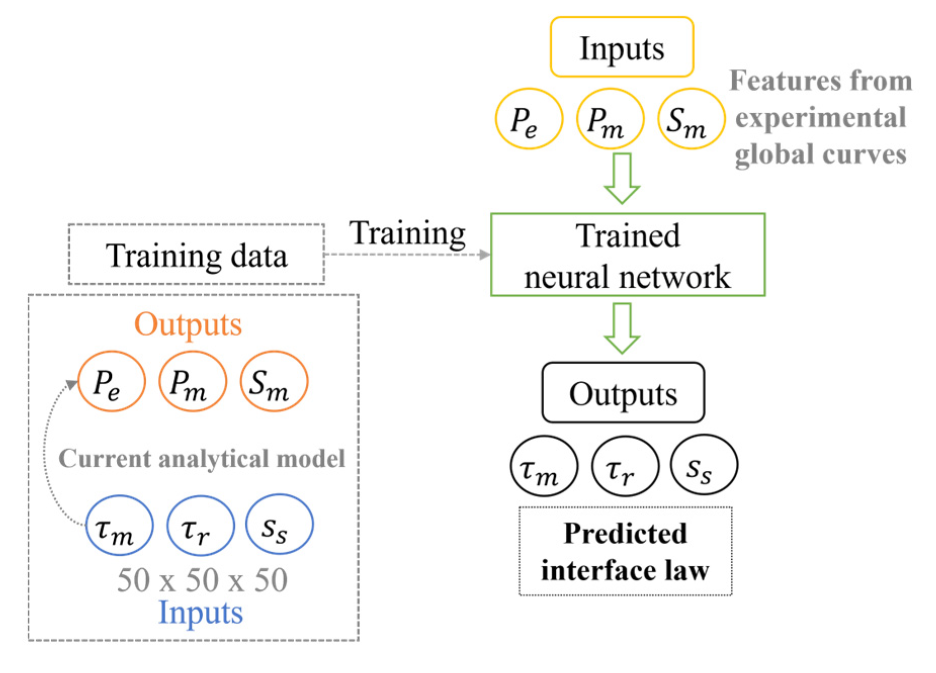
For the specific issue of inverse calibration, the data for training are structured as follows: (i) the training outputs encompass the various combinations of the parameters of the bond-slip law; (ii) the inputs for the training involve features extracted from the global curves, utilizing the aforementioned combinations within the current analytical model. Subsequently, when provided with the features of experimental global curves, the trained neural network is expected to yield the bond-slip law that corresponds to the experimental data. This process is visualized in Figure 10.

In the previous study, discussions confirmed the minor influence of the interface bond-slip law shape on the global behavior. Therefore, this section adopts a classical trilinear bond–slip relationship, requiring three parameters to be determined: ${\tau }_m$, ${\tau }_r,$ and $s_s$. The parameter $s_e$ can be directly estimated from the global curve, as it corresponds to the slip value at the end of the elastic phase. The ranges of the parameters are determined based on the previous investigation experience; ${\tau }_m$ ranges between 0.5 and 3 MPa, ${\tau }_r$ ranges between 0 and 0.5 MPa, and $s_s$ ranges between 0.1 and 0.5 mm. For each parameter range, 50 interpolations are uniformly selected, resulting in a total of ${50}^3=\mathrm{125,000}$ combinations for three parameters. In the case of intrados scenarios, only two outputs are necessary, as we assume ${\tau }_r=0$, and we will conduct 100 interpolations to generate 10,000 combinations.

Upon examining the experimentally obtained global load-slip curves presented in Figure 6, it indicates that these curves can be simplified into a two-stage polyline characterized by an initial linear phase and followed by an ascending branch. Consequently, we select three key features to serve as inputs for the neural network training. These values encompass the load and slip values at the end of the elastic branch, which are referred to as $S_e$ (known) and $P_e$, respectively, as well as the maximum load ($P_m$) and its corresponding slip ($S_m$). In conclusion, the training dataset comprises a three-dimensional input set and a corresponding three-dimensional output set for the extrados case (and a two-dimensional output set for the flat and intrados cases), resulting in a total of 125,000 items for the training (with 10,000 items allocated for the flat and intrados cases), as depicted in Figure 10.

Five neural networks were trained to infer the bond-slip law for all five cases discussed in Section 3.2, facilitated by the MATLAB Neural Network Fitting application. This versatile application enables a detailed training parameter setup and offers an effective training visualization. The preparation of the training data is accomplished through repeated calculations employing the current analytical model, where different combinations of interface law parameters are assigned. This procedure is remarkably efficient, requiring only a few minutes due to the rapid computational capabilities of the analytical model. Furthermore, the training process itself takes a matter of minutes when employing the MATLAB toolbox with the current quantity of training data. The efficiency of this approach is evident in its capacity to yield good predictions for the bond-slip laws while still demanding reasonable computational resources.

The features extracted from the experimental global curves are summarized in

Table 3. Features from experimental curves and NN predicted interface laws.

Groups	${\mathit{s}}_{\mathit{e}}$ (mm)	Inputs			NN Predicted Outputs
		${\mathit{P}}_{\mathit{e}}\left(\mathbf{k}\mathbf{N}\right)$	${\mathit{P}}_{\mathit{m}}\left(\mathbf{k}\mathbf{N}\right)$	${\mathit{S}}_{\mathit{m}}\left(\mathbf{m}\mathbf{m}\right)$	${\mathit{\tau }}_{\mathit{m}}\left(\mathbf{M}\mathbf{P}\mathbf{a}\right)$	${\mathit{\tau }}_{\mathit{r}}\left(\mathbf{M}\mathbf{P}\mathbf{a}\right)$	${\mathit{s}}_{\mathit{s}}\left(\mathbf{m}\mathbf{m}\right)$
Flat	0.040 (0.37)	5.194 (0.24)	20.397 (0.08)	1.660 (0.23)	1.436	0.184	0.253
CAE	0.036 (0.29)	6.733 (0.06)	25.895 (0.07)	2.586 (0.32)	1.491	0.297	0.415
CBE	0.019 (0.28)	5.452 (0.12)	21.811 (0.01)	3.096 (0.19)	1.758	0.106	0.186
CAI	0.036 (0.47)	5.048 (0.16)	15.916 (0.06)	0.844 (0.24)	2.118	/	0.221
CBI	0.004 (0.58)	4.848 (0.31)	16.633 (0.15)	1.844 (0.50)	2.038	/	0.228

, with corresponding standard deviations provided in brackets. The interface laws projected by the trained neural network are also presented in Table 3, and a comparison of the global curves obtained using the NN-predicted interface law and the traditional approach utilizing strain gauges is depicted in Figure 6. The results demonstrate a good predictive performance. Notably, for the flat and extrados cases, a more pronounced ascending phase and a larger maximum load can be observed due to the generation of a larger ${\tau }_r$. Nevertheless, it is important to note that, despite these promising outcomes, none of these results can fully replicate ductile behavior due to the inherent limitations in the analytical approach proposed in this study.

6. Conclusions

The present study introduced an analytical framework to describe the debonding behavior of FRP plates adhered to brittle curved substrates. A simplified classical mathematical model was employed, incorporating a multi-linear interface bond-slip law to consider the impact of normal stress induced by substrate curvature. The accuracy of the derived closed-form solutions and the effectiveness of this approach were validated against available experimental data and simulations. However, the current model exhibited brittle behavior compared to the experimental results, primarily attributed to its ignorance of the substrate. An investigation of the effects of the interface parameters confirmed that the bond behavior was primarily influenced by the interface fracture energy, rather than the specific form of the interface law. Furthermore, a novel neural-network-based approach for determining the bond-slip law in cases with absent experimental strain data was introduced, demonstrating a promising performance.