
Analysis of Cooling Load Characteristics in Chinese Residential Districts for HVAC System Design


Abstract
:1. Introduction
2. Literature Review and Research Gaps
2.1. Literature Review

| Parameter | Metric | Reference | |
|---|---|---|---|
| Peak load | Maximum value of hourly loads | [13,14] | |
| Total consumption level | Daily average load and seasonal power consumption intensity | [13,14,15] | |
| Load volatility | Daily | Hourly load profile | [18] |
where Ph is the hourly load and Pd is the daily average load | [15] | ||
where Ph is the hourly load and Pd is the daily average load | [15] | ||
| [10,13] | |||
| [10,13] | |||
| Annual relative daily variation, where Ph is the hourly average load, Pd is the daily average load and Pa is the annual average load. | [17] | ||
| Weekly | [13] | ||
| Seasonal/ annual | Load duration curve | [18] | |
where n is the total hours of load, Ph is the hourly load and Pd is the daily average load | [10] | ||
| [13] | |||
where Ph is the hourly load, Pd is the daily average load and Pa is the annual average load | [15] | ||
| Annual relative seasonal variation, where Pd is the daily average load and Pa is the annual average load. | [17] | ||
- Peak load
- Load volatility
| Parameter | Metric | Analysis Method | Reference | |
|---|---|---|---|---|
| Peak load | is the hourly load of building i at time t. | Deterministic | [22] | |
| Stochastic | [21,23] | |||
is the hourly load of building i at time t. | Deterministic | [12,21,22] | ||
| Stochastic | [24] | |||
is the hourly load of building i at time t. | Deterministic | [15] | ||
, is the hourly load of building i at time t. | Deterministic | [9] | ||
| Load volatility | Hourly load profile and load duration curve | Deterministic | [18] | |
| Daily | (mentioned in Table 1.) | Stochastic | [15] | |
| Annual | (mentioned in Table 1.) | Stochastic | [15] | |
where n. is the total hours of loads, is the normalized load and is the average value of the weighted normalized load. | Stochastic | [25] | ||
2.2. Summary and Research Gap
3. Data and Method
3.1. Data Collection
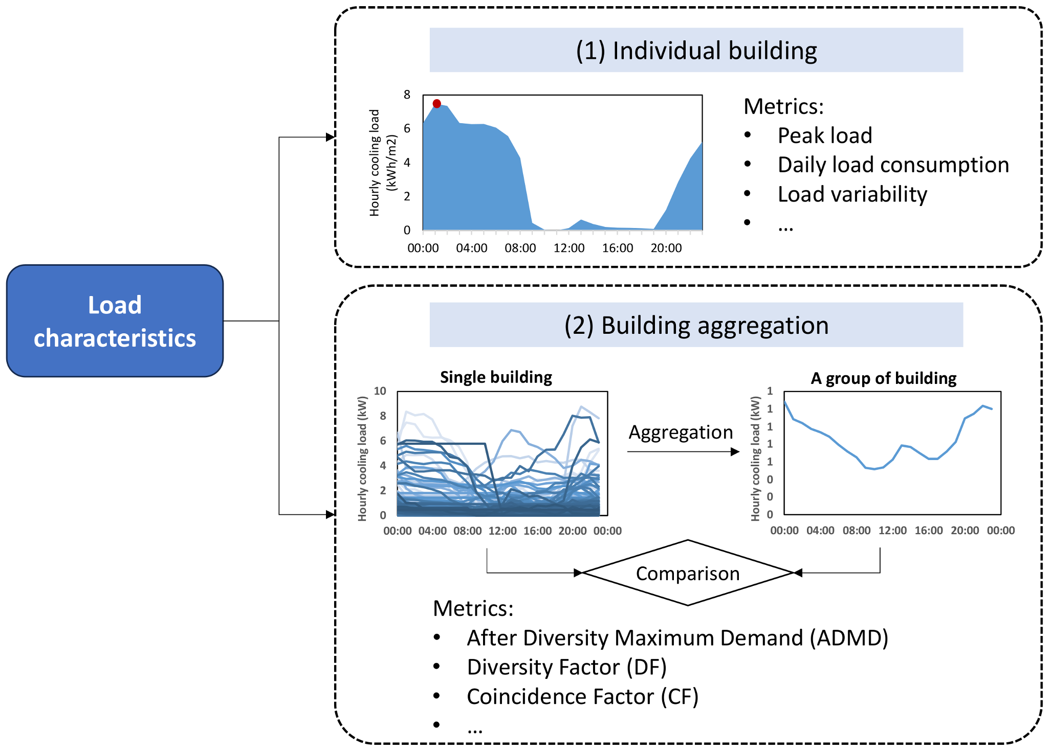
3.2. Parameters for Load Characteristics
3.3. Analysis Process
4. Analysis of Load Characteristics in a Residential District
4.1. Load Diversity among Different Households
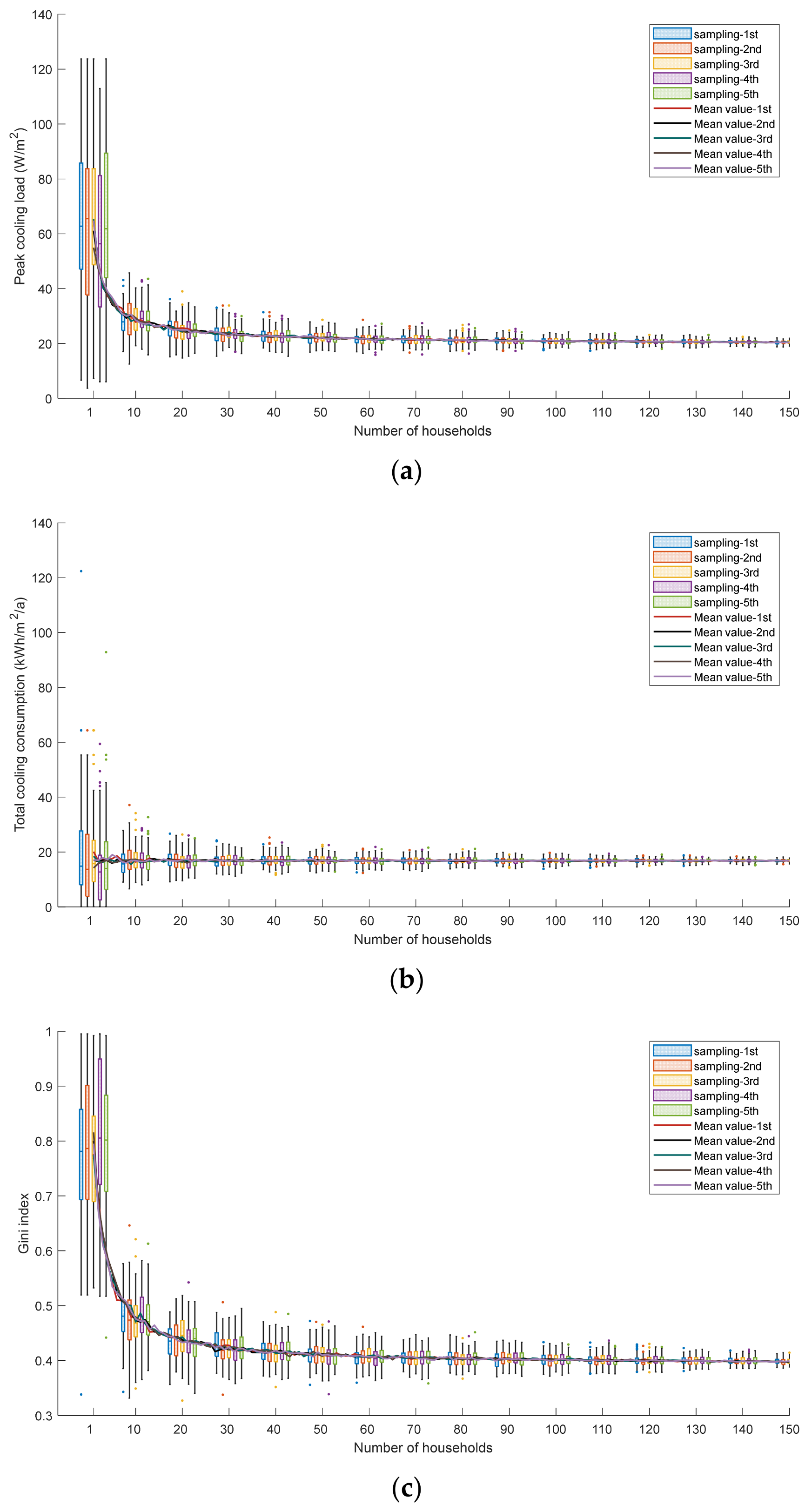
4.2. Smoothing Effect of the Cooling Loads
5. Discussion
5.1. Suggestions for HVAC System Design
5.2. Impact of Sampling Methods on the Load Characteristics
5.3. Limitations
6. Conclusions
Author Contributions
Funding
Data Availability Statement
Conflicts of Interest
References
- Building Energy Research Center in Tsinghua University. 2023 Annual Report on China Building Energy Efficiency; China Architecture & Building Press: Beijing, China, 2023. (In Chinese) [Google Scholar]
- Building Energy Research Center in Tsinghua University. 2021 Annual Report on China Building Energy Efficiency; China Architecture & Building Press: Beijing, China, 2021. (In Chinese) [Google Scholar]
- Hu, S.; Yan, D.; Guo, S.; Cui, Y.; Dong, B. A survey on energy consumption and energy usage behavior of households and residential building in urban China. Energy Build. 2017, 148, 366–378. [Google Scholar] [CrossRef]
- Li, Z.; Jiang, Y.; Wei, Q. Survey on energy consumption of air conditioning in summer in a residential building in Beijing. Heat. Vent. Air Cond. 2007, 37, 46–51. (In Chinese) [Google Scholar]
- An, J.; Yan, D.; Hong, T.; Sun, K. A novel stochastic modeling method to simulate cooling loads in residential districts. Appl. Energy 2017, 206, 134–149. [Google Scholar] [CrossRef]
- Brounen, D.; Kok, N.; Quigley, J.M. Residential energy use and conservation: Economics and demographics. Eur. Econ. Rev. 2012, 56, 931–945. [Google Scholar] [CrossRef]
- Parker, D.; Mills, E.; Rainer, L. Accuracy of the Home Energy Saver Energy Calculation Methodology. In Proceedings of the 2012 ACEEE Summer Study on Energy Efficiency in Buildings, Monterey, CA, USA, 12 August 2012; pp. 206–222. [Google Scholar]
- Gouveia, J.P.; Seixas, J. Unraveling electricity consumption profiles in households through clusters: Combining smart meters and door-to-door surveys. Energy Build. 2016, 116, 666–676. [Google Scholar] [CrossRef]
- Weissmann, C.; Hong, T.; Graubner, C.A. Analysis of heating load diversity in German residential districts and implications for the application in district heating systems. Energy Build. 2017, 139, 302–313. [Google Scholar] [CrossRef]
- Xu, L.; Pan, Y.; Lin, M.; Huang, Z. Community load leveling for energy configuration optimization: Methodology and a case study. Sustain. Cities Soc. 2017, 35, 94–106. [Google Scholar] [CrossRef]
- Kristensen, M.H.; Hedegaard, R.E.; Petersen, S. Hierarchical calibration of archetypes for urban building energy modeling. Energy Build. 2018, 175, 219–234. [Google Scholar] [CrossRef]
- Richardson, I.; Thomson, M.; Infield, D.; Clifford, C. Domestic electricity use: A high-resolution energy demand model. Energy Build. 2010, 42, 1878–1887. [Google Scholar] [CrossRef]
- Chen, S.; Zhang, X.; Wei, S.; Yang, T.; Guan, J.; Yang, W.; Qu, L.; Xu, Y. An energy planning oriented method for analyzing spatial-temporal characteristics of electric loads for heating/cooling in district buildings with a case study of one university campus. Sustain. Cities Soc. 2019, 51, 101629. [Google Scholar] [CrossRef]
- Lin, L.; Liu, X.; Zhang, T.; Liu, X.; Rong, X. Cooling load characteristic and uncertainty analysis of a hub airport terminal. Energy Build. 2021, 231, 110619. [Google Scholar] [CrossRef]
- Roberts, M.B.; Haghdadi, N.; Bruce, A.; MacGill, I. Characterisation of Australian apartment electricity demand and its implications for low-carbon cities. Energy 2019, 180, 242–257. [Google Scholar] [CrossRef]
- Vámos, V.; Horváth, M. Evaluation of district heating patterns for Hungarian residential buildings: Case study of Budapest. Energy Build. 2023, 284, 112833. [Google Scholar] [CrossRef]
- Gadd, H.; Werner, S. Heat load patterns in district heating substations. Appl. Energy 2013, 108, 176–183. [Google Scholar] [CrossRef]
- Guttromson, R.T.; Chassin, D.P.; Widergren, S.E. Residential energy resource models for distribution feeder simulation. In Proceedings of the 2003 IEEE Power Engineering Society General Meeting, Toronto, ON, Canada, 13–17 July 2003; Volume 1, pp. 108–113. [Google Scholar]
- Zhu, L.; Zhang, J.; Gao, Y.; Tian, W.; Yan, Z.; Ye, X.; Sun, Y.; Wu, C. Uncertainty and sensitivity analysis of cooling and heating loads for building energy planning. J. Build. Eng. 2022, 45, 103440. [Google Scholar] [CrossRef]
- Obrien, W.; Abdelalim, A.; Gunay, H.B. Development of an office tenant electricity use model and its application for right-sizing HVAC equipment. J. Build. Perform. Simul. 2019, 12, 37–55. [Google Scholar] [CrossRef]
- McKenna, R.; Hofmann, L.; Merkel, E.; Fichtner, W.; Strachan, N. Analysing socioeconomic diversity and scaling effects on residential electricity load profiles in the context of low carbon technology uptake. Energy Policy 2016, 97, 13–26. [Google Scholar] [CrossRef]
- Wang, Z.; Crawley, J.; Li, F.G.N.; Lowe, R. Sizing of district heating systems based on smart meter data: Quantifying the aggregated domestic energy demand and demand diversity in the UK. Energy 2020, 193, 116780. [Google Scholar] [CrossRef]
- Love, J.; Smith, A.Z.P.; Watson, S.; Oikonomou, E.; Summerfield, A.; Gleeson, C.; Biddulph, P.; Chiu, L.F.; Wingfield, J.; Martin, C.; et al. The addition of heat pump electricity load profiles to GB electricity demand: Evidence from a heat pump field trial. Appl. Energy 2017, 204, 332–342. [Google Scholar] [CrossRef]
- Clemente, S.; Beauchêne, S.; Nefzaoui, E. Generation of aggregated plug load profiles in office buildings. Energy Build. 2021, 252, 111398. [Google Scholar] [CrossRef]
- Yan, C.; Gang, W.; Niu, X.; Peng, X.; Wang, S. Quantitative evaluation of the impact of building load characteristics on energy performance of district cooling systems. Appl. Energy 2017, 205, 635–643. [Google Scholar] [CrossRef]
- Zhou, X.; Yan, D.; Feng, X.; Deng, G.; Jian, Y.; Jiang, Y. Influence of household air-conditioning use modes on the energy performance of residential district cooling systems. Build. Simul. 2016, 9, 429–441. [Google Scholar] [CrossRef]
- An, J.; Yan, D.; Hong, T. Clustering and statistical analyses of air-conditioning intensity and use patterns in residential buildings. Energy Build. 2018, 174, 214–227. [Google Scholar] [CrossRef]
- GB 50176-2016; Code for Thermal Design of Civil Building. MoHURD (Ministry of Housing and Urban-Rural Development): Beijing, China, 2016.


| Number | Parameters | Metrics | Applications |
|---|---|---|---|
| 1 | Peak cooling load | Maximum value of hourly cooling load during the cooling season | Total capacity selection of cooling devices |
| 2 | Total cooling consumption | Sum of hourly cooling load during the cooling season | Evaluation of total cooling consumption |
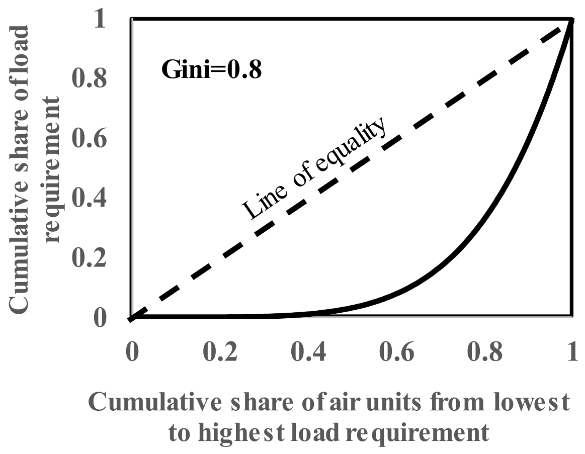
| 3 | Temporal load distribution | Gini index to evaluate the distributed load feature in a quantitative way | Selecting different combinations of cooling devices |
| 4 | Hourly load profile | Coefficient of variation to evaluate the load volatility in one day | Evaluation of control strategy of cooling devices |
Disclaimer/Publisher’s Note: The statements, opinions and data contained in all publications are solely those of the individual author(s) and contributor(s) and not of MDPI and/or the editor(s). MDPI and/or the editor(s) disclaim responsibility for any injury to people or property resulting from any ideas, methods, instructions or products referred to in the content. |
© 2023 by the authors. Licensee MDPI, Basel, Switzerland. This article is an open access article distributed under the terms and conditions of the Creative Commons Attribution (CC BY) license (https://creativecommons.org/licenses/by/4.0/).
Share and Cite
An, J.; Zhou, X.; Yan, D. Analysis of Cooling Load Characteristics in Chinese Residential Districts for HVAC System Design. Buildings 2023, 13, 2450. https://doi.org/10.3390/buildings13102450
An J, Zhou X, Yan D. Analysis of Cooling Load Characteristics in Chinese Residential Districts for HVAC System Design. Buildings. 2023; 13(10):2450. https://doi.org/10.3390/buildings13102450
Chicago/Turabian StyleAn, Jingjing, Xin Zhou, and Da Yan. 2023. "Analysis of Cooling Load Characteristics in Chinese Residential Districts for HVAC System Design" Buildings 13, no. 10: 2450. https://doi.org/10.3390/buildings13102450