A Beam Finite Element Model Considering the Slip, Shear Lag, and Time-Dependent Effects of Steel–Concrete Composite Box Beams

Abstract

A beam finite element model considering the slip, shear lag, and time-dependent effects of steel–concrete composite box beams have been proposed in this study. The element is employed to a one-dimensional analytical method that is solved involving an expression of spatial and time-dependent variables. A step-by-step method that does not involve storing the stress and strain histories, which is more accurate than the single-step algebraic method, is employed to solve the time variables. A recursive method was elaborated to determine spatial and time-dependent variables through the above method. The validity of the proposed method in instantaneous analysis is attested by the numerical data of the elaborate finite element model established in a commercial software, ANSYS, and that of the time-dependent analysis is verified by the existing test results on the long-term performance of composite beams. The proposed beam finite element model is applied to predict the time-related behavior of simply supported composite beams after validation. The results show that concrete shrinkage and creep significantly influence the structural responses of the composite box beams. From the initial load on the 28th day to that in the 3rd year, the vertical deflection at the cross-section of the mid-span increased by 47.01%. The interface slip at the end increased by −10.99%. The warping intensity function of the concrete slab and the steel beam at the end caused by shear lag increased by 111.64% and 7.01%, respectively. The maximum compressive stress on the concrete slab and the maximum tensile stress at the steel bottom flange increased by −6.75% and 4.56%, respectively.

1. Introduction

Steel-concrete composite beams, by far, have been employed into buildings and bridges world-wide. Design analysis and computational modeling of composite beams have long been active study areas [1,2,3,4,5]. Their concrete slab and steel beam are subjected to pressure and tension, respectively, under vertical loading, fully utilizing the good compressive strength of concrete and the excellent tensile strength of steel. The shear connectors serve as a kind of connection between the steel beam and the concrete slab to achieve the overall working performance. However, deformation of the shear connectors causes interface slip between the concrete slab and the steel beam, which reduces the bending stiffness of the composite beams. Actually, the interface slip concerns are characteristic not only of classical composite beams, but also of non-standard composite beams such as hybrid trussed beams with inclined shear studs [6,7]. Additionally, the shear lag effect on the slab causes varying stress distribution, remarkably for composite beams with an extremely wide concrete slab where the shear lag is positive or negative [8,9,10,11]. In the positive case, the stress at the slab–beam intersection is more than that for the remainder of the slab, while in the negative case, the stress is lower than that for the remainder of the slab. Due to the non-uniform distribution of stresses, disregarding the shear lag may bring out underestimation of the actual stresses in parts of the concrete slab. Subsequently, to simulate the mechanical behavior of composite beams accurately, the shear lag and interface slip must be taken into consideration. Figure 1 shows the two mechanical behaviors of the composite box beam above. On top of the mentioned spatial kinematic effects, the time-dependent effect of the structure because of the shrinkage and creep of the concrete slab have been a major focus in the study of composite beams, where creep and shrinkage of concrete lead the extra internal force and deformation of the composite beam to continuously change as time goes by [12,13]. Some studies have focused on the partial time-dependent effects of the composite beams. For example, D Huang et al. [14] studied the time-dependent shear lag of assembled composite beams with the concrete age difference across the section. Souici et al. [15] proposed a method to study the effects of creep in composite beams, which assumes a perfect connection between the concrete slab and the steel beam. Based on generalized beam theory, Henriques et al. [16] proposed a finite element to analyze the time-dependent effects of steel–concrete composite beams without considering the slip.

One-dimensional models that consider interface slip, shear lag, and time-dependent behaviors [17,18,19,20,21] have been widely utilized in the behavior of composite beam’s analyses. The one-dimensional beam model retains the longitudinal direction (along the span) and the cross-sectional characteristics are simplified in the transverse and vertical directions, which is obviously more efficient than the three-dimensional elaborate model. The correctness and applicability of the one-dimensional model have been widely verified by plenty of engineering practices.

The spatial and time-dependent variables are predicted to analyze one-dimensional models. To solve the spatial variables, displacement functions and the intensity functions of the entire beam are substituted into equations about virtual work. The finite element method (FEM) [20] is often utilized to solve the equations. Madenci et al. conducted some studies on finite element models of GFRP composite beams [22,23,24,25]. How to consider time variables is the main focus of the model. Many studies have considered the time-dependent behavior of composite beams due to the creep and shrinkage of concrete [26,27,28,29,30,31,32,33,34,35,36]. For the shrinkage, since the shrinkage has little to do with the stress state, the initial strain is applied to the structure during the calculation, which is simpler to address. For the creep, this is more complicated since the concrete creep is inextricably relevant to the current stress state, and the stress state in the whole stress history, which explains why many studies focus on it.

Common solutions for time variables in the literature are general step-by-step methods and methods using single-step algebraic equations. The time-integration procedures are an essential part in numerical solution procedures that translate genetic integration relations into constitutive relations for the time decomposition that can be easily addressed in the solution algorithm. Methods using one-step algebraic equations, such as the effective modulus (EM) [26], mean stress (MS) [27], and age-adjusted effective modulus (AAEM) [28,29] methods, can be used for different varieties of orthogonal formulas used for numerical integration, disregarding stress histories, but they lose the accuracy. Instead, Bazant [30] proposed a general step-by-step method aimed at this numerical integration based on the trapezoidal or midpoint rule. The drawback, however, is that the stress history as a whole needs to be restored during the solving process, which leads to a long solving time and high computational cost. However, the problem has been subsequently solved by Bazant and Wu [31]. They proposed a new strategy for the step-by-step integration methods by introducing the Dirichlet series to fit the creep function, which only requires storing the stress and strain of the previous steps in time histories. This work paves a good numerical way for the accurate analysis of the structural time-dependent behavior while saving memory and improving computational efficiency.

The above findings show that without storing data on the stress history, the step-by-step method in the time history and the finite beam element method with additional degrees of freedom (DOFs) function based on the Euler Bernoulli beam in the space provide the most accurate prediction of the complex spatial time-dependent behavior of composite beams. The novelty of the study is to propose a one-dimension theoretical model of a composite box beam considering slip, shear lag, and time-dependence based on the virtual work principle. For the solution to this model, a finite element discretization method is employed for the spatial variables, and an incremental step-by-step method without storing stress and strain histories is utilized for the time variables. A beam element with 18 DOFs for the steel–concrete composite box beam is proposed. The accuracy of the proposed beam model is verified by numerical simulations and some classical tests. Among them, the instantaneous behavior of the model is verified by numerical calculations using the finite element model, and the time-dependent behavior of the model is verified by long-term performance test results.

2. Theoretical Model of the Composite Box Beam

2.1. Principal Knowledge

The beam element model was built on the basis of the classical Euler Bernoulli beam theory and the virtual work principle. Considering the behaviors of the steel–concrete composite box beam, the following basic assumptions are made for the theoretical derivation and modeling:

(i)

The vertical bending curvatures and transverse bending curvatures of the concrete slab and steel beam are identical;

(ii)

The deflections of the concrete slab and steel beam in both vertical and transverse deflections are identical;

(iii)

Shear deformation of the beam caused by bending is disregarded;

(iv)

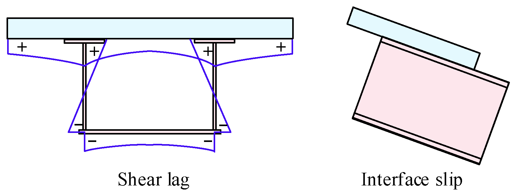
The slip between the steel beam and the concrete slab is considered only in a longitudinal direction. The shear connections are arranged uniformly along the span so that the shear connection stiffness of the interface remains identical along the span;

(v)

The shear lag on vertical deflection is considered;

(vi)

The study only focused on the structure in the normal service stage, so the concrete slab is always under elastic stage. The concrete creep is simulated by use of a linear creep model according to Bazant’s study.

(vii)

The study only focused on the structure in the normal service stage, so the steel beam is always under the elastic stage;

(viii)

The study only focused on the mechanical properties in the normal service stage, so the shear connections are always under elastic stage.

Figure 2 shows the definition of the geometrical parameters of the I-beam or box combination beam, where O_c is the centroid of the concrete slab, O_s is the centroid of the steel beam, and C_s is the torsional centroid of the transformed section of the composite beam.

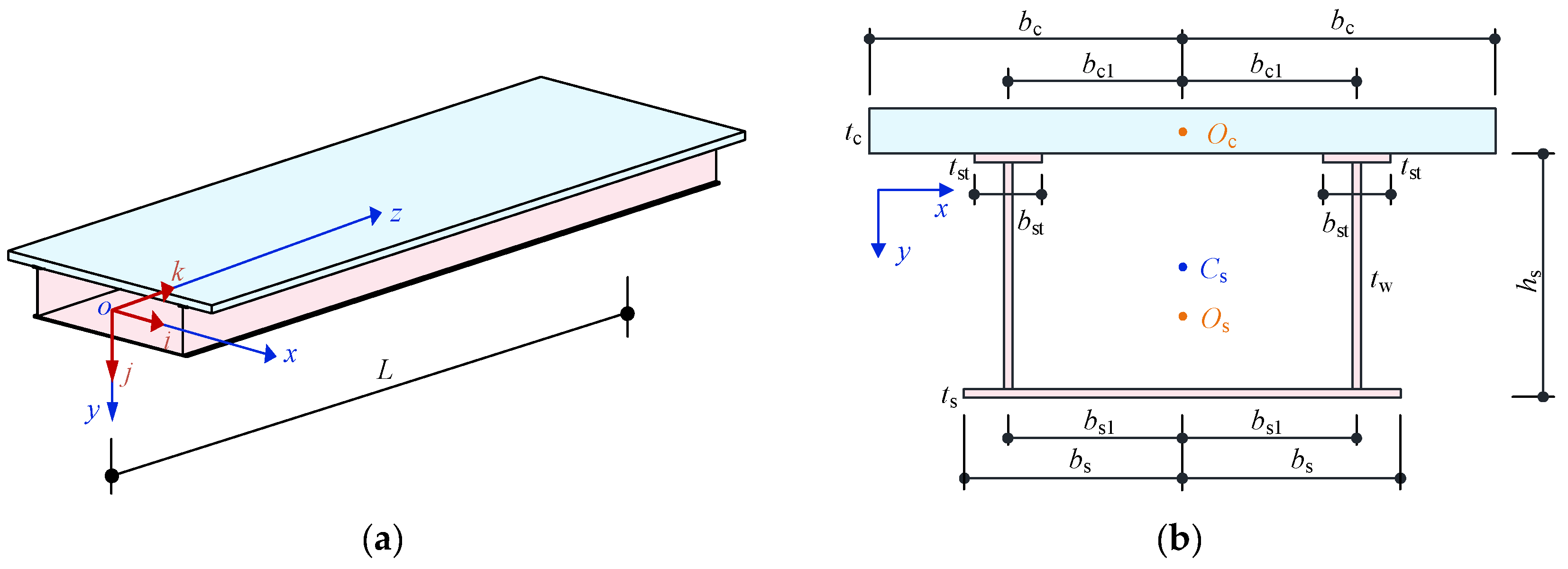
2.2. Kinematics of the Composite Box Beam

From the above assumptions and the coordinate system in Figure 2, the transverse displacement u(x, y, z) and vertical displacement v(x, y, z) at any point of the beam, displacement of the concrete slab w_c(x, y, z), and displacement of the steel beam w_s(x, y, z) in longitudinal direction are expressed as follows:

$$\left\{\begin{array}{l}u\left(x,y,z\right)=u_0\left(z\right)-\varphi \left(z\right)\left(y-y_{\mathrm{h}}\right)\\ v\left(x,y,z\right)=v_0\left(z\right)+\varphi \left(z\right)\left(x-x_{\mathrm{h}}\right)\\ w_{\mathrm{c}}\left(x,y,z\right)=w_{\mathrm{c}0}\left(z\right)-u_0^{\prime }\left(z\right)x-v_0^{\prime }\left(z\right)y+f_{\mathrm{c}}\left(z\right){\psi }_{\mathrm{c}}\left(x\right)\\ w_{\mathrm{s}}\left(x,y,z\right)=w_{\mathrm{s}0}\left(z\right)-u_0^{\prime }\left(z\right)x-v_0^{\prime }\left(z\right)y+f_{\mathrm{s}}\left(z\right){\psi }_{\mathrm{s}}\left(x\right)\end{array}\right.$$

(1)

where y_h is the y-directional coordinate of C_s; x_h is the x-directional coordinate of C_s; w_c0 and w_s0 are the longitudinal displacements of O_c and O_s, respectively; u₀ is the transverse displacement of O_c or O_s; v₀ is the vertical displacement of O_c or O_s; ϕ is the torsion angle of the overall structure; f_c and f_s are the intensity functions of warping due to shear lag on the concrete slab and steel beam, respectively; and ψ_c(x) and ψ_s(x) are the functions of warping due to shear lag on the concrete slab and steel beam, respectively. The functions of warping on the concrete slab are calculated based on Equation (2). For the steel U-beam, there is no warpage due to shear lag in the upper flange and web; thus, ψ_s(x) = 0. For the bottom flange of the steel beam, the shear lag needs to be considered and is calculated by Equation (3).

$${\psi }_{\mathrm{c}}(x)=\left\{\begin{array}{l}\left[1-{\left(\frac{b_{\mathrm{c}}-\left|x\right|}{b_{\mathrm{c}}-b_{\mathrm{c}1}}\right)}^2\right]{\left(\frac{b_{\mathrm{c}}-b_{c1}}{b_{\mathrm{c}1}}\right)}^2 \left|x\right|>b_{c1}\\ 1-{\left(\frac{\left|x\right|}{b_{\mathrm{c}}}\right)}^2 \hspace{1em}\hspace{1em}\hspace{1em}\hspace{1em}\left|x\right|\le b_{\mathrm{c}1}\end{array}\right.$$

(2)

$${\psi }_{\mathrm{s}}(x)=\left\{\begin{array}{l}1-{\left(\frac{\left|x\right|}{b_{\mathrm{s}1}}\right)}^2\hspace{1em}\hspace{1em}\left|x\right|\le b_{\mathrm{s}1} \mathrm{for} \mathrm{bottom} \mathrm{plate} \mathrm{of} \mathrm{steel} \mathrm{girder} \\ 0 \hspace{1em}\hspace{1em}\hspace{1em}\hspace{1em}\hspace{1em}\left|x\right|>b_{\mathrm{s}1} \mathrm{for} \mathrm{bottom} \mathrm{plate} \mathrm{of} \mathrm{steel} \mathrm{girder}\\ 0\hspace{1em}\hspace{1em}\hspace{1em}\hspace{1em}\hspace{1em} \mathrm{top} \mathrm{plate} \mathrm{and} \mathrm{web} \mathrm{of} \mathrm{steel} \mathrm{girder}\end{array}\right.$$

(3)

The magnitude of interface slippage between the steel beam and the concrete slab d_sl is:

$$d_{sl}\left(z\right)=w_{\mathrm{s}0}\left(z\right)-w_{\mathrm{c}0}\left(z\right)+v_0^{\prime }\left(z\right)h_0$$

(4)

where h₀ is the vertical distance between O_c and O_s.

From the variables of the displacement of the concrete slab, the normal strain ε_c and shear strain γ_c of the concrete slab are obtained:

$$\left\{\begin{array}{l}{\epsilon }_{\mathrm{c}}\left(x,y,z\right)=w_{\mathrm{c}0}^{\prime }\left(z\right)-u_0^{″}\left(z\right)x-v_0^{″}\left(z\right)y+f_{\mathrm{c}}^{\prime }\left(z\right){\psi }_{\mathrm{c}}\\ {\gamma }_{\mathrm{c}}\left(x,y,z\right)={\varphi }^{\prime }\left(z\right)r_{\mathrm{c}}^{\ast }+f_{\mathrm{c}}\left(z\right){\psi }_{\mathrm{c},x}\end{array}\right.$$

(5)

From the displacement variables of the steel beam, the normal strain ε_s and tangential strain γ_s of the steel beam are obtained:

$$\left\{\begin{array}{l}{\epsilon }_{\mathrm{s}}\left(x,y,z\right)=w_{\mathrm{s}0}^{\prime }\left(z\right)-u_0^{″}\left(z\right)x-v_0^{″}\left(z\right)y+f_{\mathrm{s}}^{\prime }\left(z\right){\psi }_{\mathrm{s}}\\ {\gamma }_{\mathrm{s}}\left(x,y,z\right)={\varphi }^{\prime }\left(z\right)r_{\mathrm{s}}^{\ast }+f_{\mathrm{s}}\left(z\right){\psi }_{\mathrm{s},x}\end{array}\right.$$

(6)

where $r_{\mathrm{c}}^{\ast }$ is the vertical distance from C_s to any point of the concrete slab along its thin wall and $r_{\mathrm{s}}^{\ast }$ is the vertical distance from C_s to any point of the steel beam along its thin wall of. ψ_c,x is the derivative of ψ_c of x in first order, and ψ_s,x is the first-order derivative of ψ_s with respect to x.

2.3. Virtual Work of the Composite Box Beam

The one-dimensional analysis model of the composite box beam is on the basis of the virtual work principle where the expression is:

$$\begin{array}{l}\mathsf{\delta }\mathrm{\Pi }={\displaystyle \underset{L}{\int }{\displaystyle \underset{A_{\mathrm{c}}}{∯}\mathsf{\delta }{\mathsf{\epsilon }}_c^{\mathrm{T}}{\mathsf{\sigma }}_{\mathbf{c}}\mathrm{d}a}\mathrm{d}z}+{\displaystyle \underset{L}{\int }{\displaystyle \underset{A_{\mathrm{s}}}{∯}\mathsf{\delta }{\mathsf{\epsilon }}_{\mathrm{s}}^{\mathrm{T}}{\mathsf{\sigma }}_{\mathrm{s}}\mathrm{d}a}\mathrm{d}z}+{\displaystyle \underset{L}{\int }{\mathsf{\delta }d}_{\mathrm{sl}}{q}_{\mathrm{sl}}\mathrm{d}z}-{\displaystyle \sum \mathsf{\delta }{\mathbf{W}}^{\mathbf{T}}\mathbf{Q}}-{\displaystyle \underset{L}{\int }\mathsf{\delta }{\mathbf{W}}^{\mathrm{T}}\mathbf{q}\mathrm{d}z}=0\\ \forall \mathsf{\delta }{\mathsf{\epsilon }}_{\mathrm{s}},\mathsf{\delta }{\mathsf{\epsilon }}_{\mathbf{c}},\mathsf{\delta }{q}_{\mathrm{sl}},\mathsf{\delta }\mathbf{W}\end{array}$$

(7)

where A_s and A_c are the areas of the steel beam and concrete slab cross-section, respectively, and L is the length of the composite beam span. In order to present the results concisely, the variables and equations are subsequently expressed as a matrix.

(1) 

Internal virtual work of the steel beam and the concrete slab

${\displaystyle \underset{L}{\int }{\displaystyle \underset{A_{\mathrm{c}}}{∯}\mathsf{\delta }{\mathsf{\epsilon }}_{\mathbf{c}}^{\mathrm{T}}{\mathsf{\sigma }}_{\mathbf{c}}\mathrm{d}a}\mathrm{d}z}$ and ${\displaystyle \underset{L}{\int }{\displaystyle \underset{A_{\mathrm{s}}}{∯}\mathsf{\delta }{\mathsf{\epsilon }}_{\mathrm{s}}^{\mathrm{T}}{\mathsf{\sigma }}_{\mathrm{s}}\mathrm{d}a}\mathrm{d}z}$ in Equation (7) represent the internal virtual work caused by the deformation of the concrete slab and the steel beam, separately. ε_c is the strain matrix of the concrete slab, as shown in Equation (8), which includes the normal strain and tangential strain, respectively.

$${\mathsf{\epsilon }}_{\mathbf{c}}={\left(\begin{array}{cc}{\epsilon }_c& {\gamma }_c\end{array}\right)}^{\mathrm{T}}$$

(8)

The strain matrix ε_c of a concrete slab is:

$${\mathsf{\epsilon }}_{\mathbf{c}}={\mathbf{B}}_{\mathbf{c}}{\mathbf{d}}_{\mathbf{c}}$$

(9)

where

$${\mathbf{B}}_{\mathbf{c}}=\left(\begin{array}{cccccc}-x& -y& 1& {\psi }_{\mathrm{c}}& 0& 0\\ 0& 0& 0& 0& r_{\mathrm{c}}^{\ast }& {\psi }_{\mathrm{c},x}\end{array}\right)$$

(10)

$${\mathbf{d}}_{\mathbf{c}}={\left(\begin{array}{cccccc}{u}_0^{″}& v_0^{″}& w_{\mathrm{c}0}^{\prime }& f_{\mathrm{c}}^{\prime }& {\varphi }^{\prime }& f_{\mathrm{c}}\end{array}\right)}^{\mathrm{T}}$$

(11)

ε_s is the strain matrix of the steel beam, as shown in Equation (12), including normal strain and tangential strain, respectively.

$${\mathsf{\epsilon }}_{\mathbf{s}}={\left(\begin{array}{cc}{\epsilon }_s& {\gamma }_s\end{array}\right)}^{\mathrm{T}}$$

(12)

The strain matrix of steel beam ε_s is:

$${\mathsf{\epsilon }}_{\mathbf{s}}={\mathbf{B}}_{\mathbf{s}}{\mathbf{d}}_{\mathbf{s}}$$

(13)

where

$${\mathbf{B}}_{\mathbf{s}}=\left(\begin{array}{cccccc}-x& -y& 1& {\psi }_{\mathrm{s}}& 0& 0\\ 0& 0& 0& 0& r_{\mathrm{c}}^{\ast }& {\psi }_{\mathrm{s},x}\end{array}\right)$$

(14)

$${\mathbf{d}}_{\mathbf{s}}={\left(\begin{array}{cccccc}{u}_0^{″}& v_0^{″}& w_{\mathrm{s}0}^{\prime }& f_{\mathrm{s}}^{\prime }& {\varphi }^{\prime }& f_{\mathrm{s}}\end{array}\right)}^{\mathrm{T}}$$

(15)

The stress matrix of the concrete slab σ_c (Equation (16)) including normal stress σ_c and tangential stress τ_c:

$${\mathsf{\sigma }}_{\mathbf{c}}={\left(\begin{array}{cc}{\sigma }_c& {\tau }_c\end{array}\right)}^{\mathrm{T}}$$

(16)

Based on assumption (vi), considering the shrinkage and creep effect of concrete, introduce the creep function J(t,t₀) and shrinkage strain matrix ε_c,sh(t). The relationship between the stress and the strain of concrete is expressed as follows:

$${\mathsf{\epsilon }}_{\mathbf{c}}\left(t\right)-{\mathsf{\epsilon }}_{\mathbf{c},\mathbf{s}\mathbf{h}}\left(t\right)=J\left(t,t_0\right){\mathbf{X}}_{\mathbf{c}}^{-1}{\mathsf{\sigma }}_{\mathbf{c}}\left(t_0\right)+{\displaystyle {\int }_{t_0}^{t}J\left(t,\tau \right){\mathbf{X}}_{\mathbf{c}}^{-1}\mathrm{d}{\mathsf{\sigma }}_{\mathbf{c}}\left(\tau \right)}$$

(17)

where t is the age of concrete, t₀ is the initial loading age of concrete, and ε_c,sh is the matrix of instantaneous shrinkage strain of concrete with respect to t (Equation (18)). ε_c,sh(t) in Equation (18) is the instantaneous shrinkage strain of concrete with respect to t. The relationship X_c is shown in Equation (19), and μ_c in Equation (19) is Poisson’s ratio of concrete.

$${\mathsf{\epsilon }}_{\mathbf{c},\mathbf{s}\mathbf{h}}={\left(\begin{array}{cc}{\epsilon }_{\mathrm{c},\mathrm{s}\mathrm{h}}& 0\end{array}\right)}^{\mathrm{T}}$$

(18)

$${\mathbf{X}}_{\mathbf{c}}=\left(\begin{array}{cc}1& 0\\ 0& \frac{1}{2\left(1+{\mu }_{\mathrm{c}}\right)}\end{array}\right)$$

(19)

The stress matrix of the steel beam σ_s (Equation (20)) comprises the normal stress σ_s and shear stress τ_s.

$${\mathsf{\sigma }}_{\mathbf{s}}={\left(\begin{array}{cc}{\sigma }_{\mathrm{s}}& {\tau }_{\mathrm{s}}\end{array}\right)}^{\mathrm{T}}$$

(20)

According to assumption (vii), the relationship between σ_s and ε_s is:

$${\mathsf{\sigma }}_{\mathbf{s}}=E_{\mathrm{s}}{\mathbf{X}}_{\mathbf{s}}{\mathsf{\epsilon }}_{\mathbf{s}}$$

(21)

where the relationship X_s is shown in Equation (22), E_s is the elastic modulus of steel, and μ_s is Poisson’s ratio of steel.

$${\mathbf{X}}_{\mathbf{s}}=\left(\begin{array}{cc}1& 0\\ 0& \frac{1}{2\left(1+{\mu }_{\mathrm{s}}\right)}\end{array}\right)$$

(22)

(2) 

Internal virtual work by interface slip

${\displaystyle \underset{L}{\int }{\mathsf{\delta }d}_{\mathrm{sl}}{q}_{\mathrm{sl}}\mathrm{d}z}$ in Equation (7) is the internal virtual work due to the interface slip between the steel beam and the concrete slab. From the assumption (viii), the relationship between the interface shear force d_sl and the interface slip displacement q_sl is expressed as follows:

$$q_{\mathrm{sl}}\left(z\right)=\rho d_{\mathrm{sl}}\left(z\right)$$

(23)

where ρ is the per unit length along the longitudinal direction for the shear connection stiffness of the interface.

(3) 

External virtual work

${\displaystyle \sum \mathsf{\delta }{\mathbf{W}}^{\mathrm{T}}\mathbf{Q}}$ in Equation (7) is the external virtual work due to the concentrated load at any position of the composite beam, and ${\displaystyle \underset{L}{\int }\mathsf{\delta }{\mathbf{W}}^{\mathrm{T}}\mathbf{q}\mathrm{d}z}$ is the external virtual work due to the distributed load at any position of the composite beam.

According to Equation (1), the displacement vector W at any position of the steel beam or the concrete slab is expressed as:

$$\mathbf{W}={\left(\begin{array}{cccc}u\left(x,y,z\right)& v\left(x,y,z\right)& w_{\mathrm{c}}\left(x,y,z\right)& w_{\mathrm{s}}\left(x,y,z\right)\end{array}\right)}^{\mathrm{T}}$$

(24)

Furthermore, Equation (24) is written as:

$$\mathbf{W}=\mathbf{H}{\mathbf{d}}_{\mathbf{F}}$$

(25)

where

$$\mathbf{H}=\left(\begin{array}{ccccccccc}1& 0& 0& 0& 0& 0& -\left(y-y_{\mathrm{Cs}}\right)& 0& 0\\ 0& 0& 1& 0& 0& 0& x-x_{\mathrm{Cs}}& 0& 0\\ 0& -x& 0& -y& 1& 0& 0& {\psi }_{\mathrm{c}}& 0\\ 0& -x& 0& -y& 0& 1& 0& 0& {\psi }_{\mathrm{s}}\end{array}\right)$$

(26)

$${\mathbf{d}}_{\mathrm{F}}={\left(\begin{array}{ccccccccc}{u}_0& u_0^{\prime }& v_0& v_0^{\prime }& w_{\mathrm{c}0}& w_{\mathrm{s}0}& \varphi & f_{\mathrm{c}}& f_{\mathrm{s}}\end{array}\right)}^{\mathrm{T}}$$

(27)

The concentrated load Q and distributed load q are expressed as follows:

$$\mathbf{Q}={\left(\begin{array}{cccc}{Q}_x& Q_y& Q_{\mathrm{c}z}& Q_{\mathrm{s}z}\end{array}\right)}^{\mathrm{T}}$$

(28)

$$\mathbf{q}={\left(\begin{array}{cccc}{q}_x& q_y& q_{\mathrm{c}z}& q_{\mathrm{s}z}\end{array}\right)}^{\mathrm{T}}$$

(29)

where Q_x, Q_y, and Q_z are the concentrated loads in the x, y, and z direction, respectively, and q_x, q_y, and q_z are the distributed loads in the x, y, and z direction, respectively. It should be noted that this analytical model considers the case that the load acts at any position.

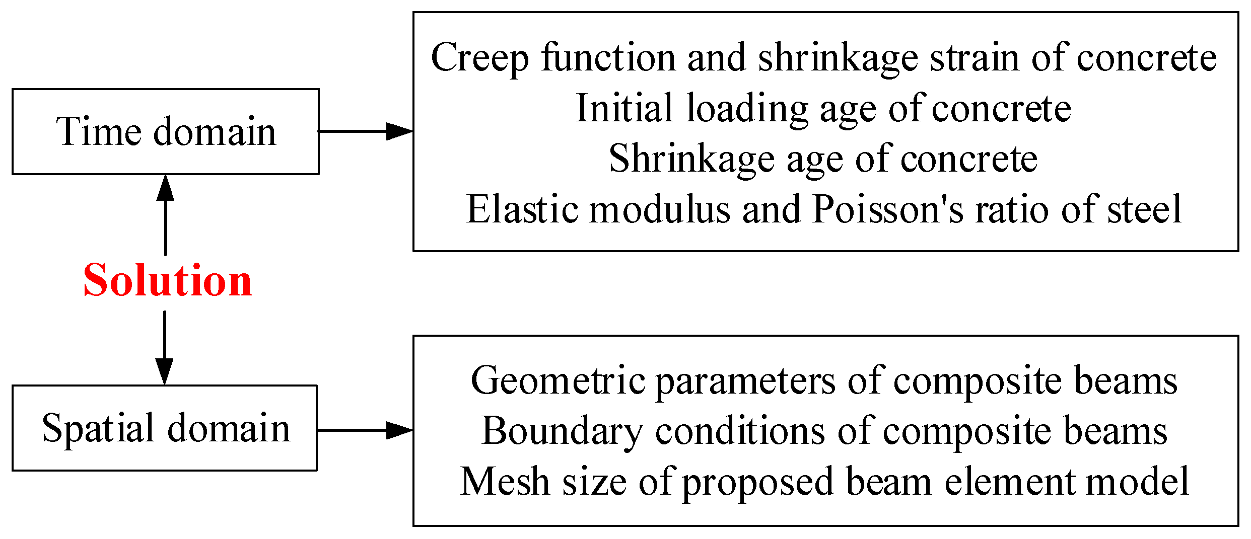
3. Numerical Procedure of the Analysis Model

The one-dimensional theoretical model of the composite box beam includes two parts as follows. First, the time-dependent components are obtained using a more accurate step-by-step method. To save computational space (without storing the stress history), the Dirichlet series is introduced to the creep function. Second, the space-related components are obtained by the FEM selected to discretize the composite box beam into several beam elements with two nodes. Next, the components of element stiffness and equivalent load matrices at each node are calculated, which are applied to obtain the overall stiffness matrix and the overall equivalent load matrix.

3.1. Time Integration: Incremental Step-by-Step Method without Storing the Histories of Stress and Strain

When the effect of temperature on concrete is disregarded, the gross strain of concrete is the combination of strain, shrinkage strain, and creep strain in an instant [34], as shown in Equation (30). The shrinkage strain is not related to the forces of the structure, and the numerical model of the overall structure equals to the initial strain of the composite box beam when considering shrinkage, which is a relatively simple method to address. The instantaneous strain and creep strain are related to the forces of the structure. Moreover, the strain is related to the stress, both of which change over time. So, the numerical analysis of this process is far more cumbersome. According to reference [34], the creep function J(t, t₀) is employed to obtain the instantaneous strain and creep strain.

$${\mathsf{\epsilon }}_{\mathbf{c}}\left(t\right)={\mathsf{\epsilon }}_{\mathbf{c},\mathbf{e}}\left(t\right)+{\mathsf{\epsilon }}_{\mathbf{c},\mathbf{s}\mathbf{h}}\left(t\right)+{\mathsf{\epsilon }}_{\mathbf{c},\mathbf{c}\mathbf{r}}\left(t\right)$$

(30)

According to reference [34], the creep function is written in the form of Equation (31):

$$J\left(t,t_0\right)=\frac{1}{E_{\mathrm{c}}\left(t\right)}+C\left(t,t_0\right)$$

(31)

where E_c(t) is the elastic modulus of concrete in each time step t, and C(t,t₀) is the specific creep function of concrete in each time step t when the initial loading age is t₀. By substituting Equation (31) into Equation (17) and separating the instantaneous strain ε_c,e(t) and creep strain ε_c,cr(t), the following expressions are obtained:

$${\mathsf{\epsilon }}_{\mathbf{c},\mathbf{e}}\left(t\right)={\mathbf{X}}_{\mathbf{c}}^{-1}\frac{{\mathsf{\sigma }}_{\mathbf{c}}\left(t\right)}{E_{\mathrm{c}}\left(t\right)}={\mathbf{X}}_{\mathbf{c}}^{-1}\frac{{\mathsf{\sigma }}_{\mathbf{c}}\left(t_0\right)}{E_{\mathrm{c}}\left(t_0\right)}+{\displaystyle {\int }_{t_0}^t\frac{1}{E_{\mathrm{c}}\left(\tau \right)}{\mathbf{X}}_{\mathbf{c}}^{-1}\mathrm{d}{\mathsf{\sigma }}_{\mathbf{c}}\left(\tau \right)}$$

(32)

$${\mathsf{\epsilon }}_{\mathbf{c},\mathbf{c}\mathbf{r}}\left(t\right)={\mathbf{X}}_{\mathbf{c}}^{-1}{\mathsf{\sigma }}_{\mathbf{c}}\left(t_0\right)C\left(t,t_0\right)+{\displaystyle {\int }_{t_0}^{t}C\left(t,\tau \right)}{\mathbf{X}}_{\mathbf{c}}^{-1}\mathrm{d}{\mathsf{\sigma }}_{\mathbf{c}}\left(\tau \right)$$

(33)

To improve the accuracy as much as possible, the incremental step-by-step method is adopted, and the Dirichlet series is employed into the specific creep function C(t, t₀) by the step-by-step method (without storing the stress and strain histories, respectively). According to reference [34], the Dirichlet series expansion of C(t, t₀) in Equation (31) is shown in Equation (34), i.e., the Kabir formula:

$$C\left(t,t_0\right)={\displaystyle \sum _{j=1}^m{\alpha }_j\left(t_0\right)\left(1-e^{-\left(t-t_0\right)/{\tau }_j}\right)}$$

(34)

Bazant [34] suggested that for the concrete creep problem, using m = 4 is sufficient to guarantee the validity of the expansion of series, and the delay time τ_j = 10^j−1 (j = 1, 2, …, m). The α_j(t₀) (i = 1, 2, …, m) in Equation (34) is solved by the least-squares method provided that C(t, t₀) is known.

To apply the incremental step-by-step method, the time step from t₀ to t is discretized in the form of Δt_n = t_n − t_n−1 (n ≥ 1), and $\Delta {\mathsf{\epsilon }}_{\mathbf{c}}^n$, $\Delta {\mathsf{\epsilon }}_{\mathbf{c},\mathbf{c}\mathbf{r}}^n$, $\Delta {\mathsf{\epsilon }}_{\mathbf{c},\mathbf{s}\mathbf{h}}^n$ and $\Delta {\mathsf{\sigma }}_{\mathbf{c}}^n$ of Δt_n are solved. Among these variables, $\Delta {\mathsf{\epsilon }}_{\mathbf{c},\mathbf{s}\mathbf{h}}^n$ is independent of stress and is obtained from the time-dependent constitutive relation of shrinkage strain; $\Delta {\mathsf{\epsilon }}_{\mathbf{c}}^n$ is obtained from the displacement matrix d_c of concrete, while the calculation of $\Delta {\mathsf{\epsilon }}_{\mathbf{c},\mathbf{c}\mathbf{r}}^n$ and $\Delta {\mathsf{\sigma }}_{\mathbf{c}}^n$ is more complicated and needs to be calculated by the recursive method [34]:

Using the nth time step Δt_n as an example, we have Equation (33):

$${\mathsf{\epsilon }}_{\mathbf{c},\mathbf{c}\mathbf{r}}^n=\left\{\begin{array}{l}{\left[\mathbf{0}\right]}_{2\times 1}n=0\\ {\mathbf{X}}_{\mathbf{c}}^{-1}{\displaystyle \sum _{i=0}^{n-1}\Delta {\mathsf{\sigma }}_{\mathbf{c}}^{i}C\left(t_n,t_i\right)}n>0\end{array}\right.$$

(35)

When n > 0,

$$\Delta {\mathsf{\epsilon }}_{\mathbf{c},\mathbf{c}\mathbf{r}}^n={\mathsf{\epsilon }}_{\mathbf{c},\mathbf{c}\mathbf{r}}^n-{\mathsf{\epsilon }}_{\mathbf{c},\mathbf{c}\mathbf{r}}^{n-1}={\mathbf{X}}_{\mathbf{c}}^{-1}\left[{\displaystyle \sum _{i=0}^{n-2}\Delta {\mathsf{\sigma }}_{\mathbf{c}}^i\left(C\left(t_n,t_i\right)-C\left(t_{n-1},t_i\right)\right)}+\Delta {\mathsf{\sigma }}_{\mathbf{c}}^{n-1}C\left(t_n,t_{n-1}\right)\right]$$

(36)

When n = 0,

$$\Delta {\mathsf{\epsilon }}_{\mathbf{c},\mathbf{c}\mathbf{r}}^0={\mathsf{\epsilon }}_{\mathbf{c},\mathbf{c}\mathbf{r}}^0={[\mathbf{0}]}_{2\times 1}$$

(37)

Therefore,

$$\Delta {\mathsf{\epsilon }}_{\mathbf{c},\mathbf{c}\mathbf{r}}^n=\left\{\begin{array}{c}{[\mathbf{0}]}_{2\times 1}n=0\\ {\mathbf{X}}_{\mathbf{c}}^{-1}\left[{\displaystyle \sum _{i=0}^{n-2}\Delta {\mathsf{\sigma }}_{\mathbf{c}}^i\left(C\left(t_n,t_i\right)-C\left(t_{n-1},t_i\right)\right)}+\Delta {\mathsf{\sigma }}_{\mathbf{c}}^{n-1}C\left(t_n,t_{n-1}\right)\right]n>0\end{array}\right.$$

(38)

In Equation (38),

$$\begin{array}{l}C\left(t_n,t_i\right)-C\left(t_{n-1},t_i\right)\\ ={\displaystyle \sum _{j=1}^m{\alpha }_j\left(t_i\right)\left[1-e^{-{\lambda }_j\left(t_n-t_i\right)/{\tau }_j}\right]}-{\displaystyle \sum _{j=1}^m{\alpha }_j\left(t_i\right)\left[1-e^{-\left(t_{n-1}-t_i\right)/{\tau }_j}\right]}\\ ={\displaystyle \sum _{j=1}^m{\alpha }_j\left(t_i\right)}\left[e^{-\left(t_{n-1}-t_i\right)/{\tau }_j}-e^{-\left(t_n-t_i\right)/{\tau }_j}\right]\\ ={\displaystyle \sum _{j=1}^m{\alpha }_j\left(t_i\right)e^{-\left(t_{n-1}-t_i\right)/{\tau }_j}}\left[1-e^{-\Delta t_n/{\tau }_j}\right]\end{array}$$

(39)

Therefore, we obtain:

$$\Delta {\mathsf{\epsilon }}_{\mathbf{c},\mathbf{c}\mathbf{r}}^n={\mathbf{X}}_{\mathbf{c}}^{-1}\left[{\displaystyle \sum _{j=1}^m{\mathsf{\beta }}_{\mathbf{j}}^n}\left(1-e^{-\Delta t_n/{\tau }_j}\right)+\Delta {\mathsf{\sigma }}_{\mathbf{c}}^{n-1}C\left(t_n,t_{n-1}\right)\right]$$

(40)

where

$${\mathsf{\beta }}_{\mathbf{j}}^n=\left\{\begin{array}{c}\Delta {\mathsf{\sigma }}_{\mathbf{c}}^0{\alpha }_j\left(t_0\right)n=1\\ {\displaystyle \sum _{i=0}^{n-1}\Delta {\mathsf{\sigma }}_{\mathbf{c}}^i{\alpha }_j\left(t_i\right)e^{-\left(t_{n-1}-t_i\right)/{\tau }_j}}n>1\end{array}\right.$$

(41)

It can be determined that ${\mathsf{\beta }}_{\mathbf{j}}^n$ satisfies the recurrence relation, as shown in Equation (42). It is only necessary to store ${\mathsf{\beta }}_{\mathbf{j}}^{n-1}$ and stress increment $\Delta {\mathsf{\sigma }}_{\mathbf{c}}^{n-1}$ at the previous time step Δt_n−1 to obtain ${\mathsf{\beta }}_{\mathbf{j}}^n$ at time step Δt_n, which avoids the need to store stress and strain histories.

$${\mathsf{\beta }}_{\mathbf{j}}^n={\mathsf{\beta }}_{\mathbf{j}}^{n-1}{e}^{-\Delta t_{n-1}/{\tau }_j}+\Delta {\mathsf{\sigma }}_{\mathbf{c}}^{n-1}{\alpha }_j\left(t_{n-1}\right)$$

(42)

Therefore, it is determined that the strain increment $\Delta {\mathsf{\epsilon }}_{\mathbf{c},\mathbf{c}\mathbf{r}}^n$ of time step Δt_n is obtained from the stress increment $\Delta {\mathsf{\sigma }}_{\mathbf{c}}^{n-1}$ of the previous time step Δt_n−1 and ${\beta }_j^n$ of the time step Δt_n. According to Equation (32), the following expressions are obtained:

$$\Delta {\mathsf{\sigma }}_{\mathbf{c}}^n={\overline{E}}_{\mathrm{c}}^n{\mathbf{X}}_{\mathbf{c}}\left(\Delta {\mathsf{\epsilon }}_{\mathbf{c}}^n-\Delta {\mathsf{\epsilon }}_{\mathbf{c},\mathbf{c}\mathbf{r}}^n-\Delta {\mathsf{\epsilon }}_{\mathbf{c},\mathbf{s}\mathbf{h}}^n\right)$$

(43)

where

$${\overline{E}}_{\mathrm{c}}^n=\left\{\begin{array}{c}{E}_{\mathrm{c}}^{n}n=0\\ E_{\mathrm{c}}^{n-0.5}n>0\end{array}\right.$$

(44)

As shown in Equation (43), the $\Delta {\mathsf{\sigma }}_{\mathbf{c}}^n$ of time step Δt_n is obtained. Afterward, one can proceed to the next time step Δt_n+1 and continue to repeat the above calculation process.

3.2. Space Integration: The Finite Beam Element with 18 DOFs

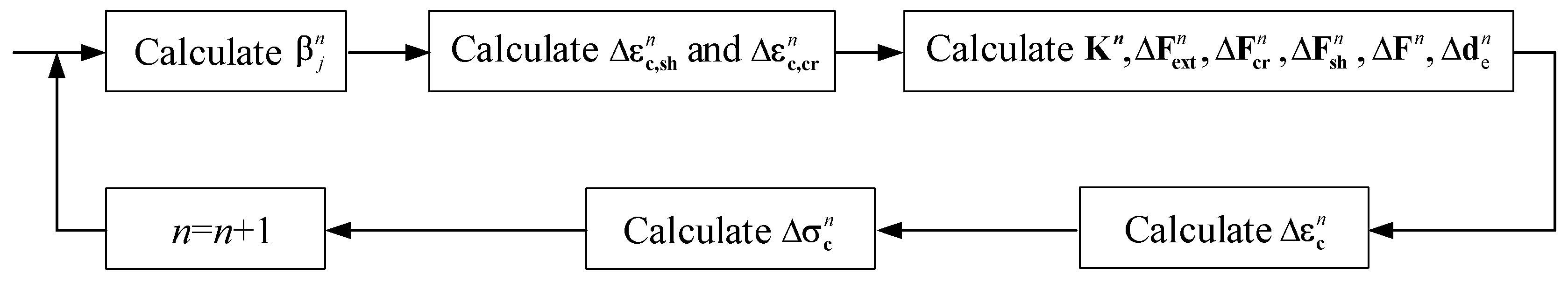
An FEM with high accuracy and stability is applied to obtain the one-dimensional analysis model in space. Like Equation (7), the identical virtual work principle is followed in incremental time steps Δt_n:

$$\begin{array}{l}\mathsf{\delta }\left(\Delta \mathrm{\Pi }\right)={\displaystyle \underset{L}{\int }{\displaystyle \underset{A_{\mathrm{c}}}{∯}\mathsf{\delta }{\mathsf{\epsilon }}_{\mathbf{c}}^{\mathrm{T}}\left(\Delta {\mathsf{\sigma }}_{\mathbf{c}}^n\right)\mathrm{d}a}\mathrm{d}z}+{\displaystyle \underset{L}{\int }{\displaystyle \underset{A_{\mathrm{s}}}{∯}\mathsf{\delta }{\mathsf{\epsilon }}_{\mathbf{s}}^{\mathrm{T}}\left(\Delta {\mathsf{\sigma }}_{\mathbf{s}}^n\right)\mathrm{d}a}\mathrm{d}z}+{\displaystyle \underset{L}{\int }\mathsf{\delta }{d}_{sl}\left(\Delta q_{\mathrm{sl}}^n\right)\mathrm{d}z}-{\displaystyle \sum \mathsf{\delta }{\mathbf{W}}^{\mathrm{T}}\left(\Delta {\mathbf{Q}}^n\right)}-{\displaystyle \underset{L}{\int }\mathsf{\delta }{\mathbf{W}}^{\mathrm{T}}\left(\Delta {\mathbf{q}}^n\right)\mathrm{d}z}=0\\ \forall \mathsf{\delta }{\mathsf{\epsilon }}_{\mathbf{s}},\mathsf{\delta }{\mathsf{\epsilon }}_{\mathbf{c}},\mathsf{\delta }{d}_{\mathrm{sl}},\mathsf{\delta }\mathbf{W}\end{array}$$

(45)

The composite box beam is discretized into two-node finite beam elements with 18 DOFs, each node containing 9 DOFs. The elements of the node displacement matrix of d_e are:

$${\mathbf{d}}_{\mathbf{e}}={\left(\begin{array}{cc}{\mathbf{d}}_{\mathbf{e}\mathbf{1}}& {\mathbf{d}}_{\mathbf{e}\mathbf{2}}\end{array}\right)}^T$$

(46)

$${\mathbf{d}}_{\mathbf{e}\mathbf{i}}=\left(\begin{array}{ccccccccc}{u}_i& {u^{\prime }}_i& v_i& {v^{\prime }}_i& w_{\mathrm{c}i}& w_{\mathrm{s}i}& {\varphi }_i& f_{\mathrm{c}i}& f_{\mathrm{s}i}\end{array}\right) \mathrm{for} i=1,2$$

(47)

Based on the node displacement matrix of element d_e, the shape function matrices [N_c]_6×18, [N_s]_6×18, [N_sl]_1×18, and [N_F]_9×18 are introduced. The following equations are obtained:

$${\mathbf{d}}_{\mathbf{c}}={\mathbf{N}}_{\mathbf{c}}{\mathbf{d}}_{\mathbf{e}}$$

(48)

$${\mathbf{d}}_{\mathbf{s}}={\mathbf{N}}_{\mathbf{s}}{\mathbf{d}}_{\mathbf{e}}$$

(49)

$$d_{sl}={\mathbf{N}}_{\mathbf{s}\mathbf{l}}{\mathbf{d}}_{\mathbf{e}}$$

(50)

$${\mathbf{d}}_{\mathbf{F}}={\mathbf{N}}_{\mathbf{F}}{\mathbf{d}}_{\mathbf{e}}$$

(51)

where the values of the shape function matrices [N_c]_6×18, [N_s]_6×18, [N_sl]_1×18, and [N_F]_9×18 are illustrated in Appendix A.

Substitute Equations (9), (13), (21), (23), (25), (43), (48), and (49) into Equation (45), and the equilibrium equation of the composite box beam at time interval Δt_n is solved as:

$${\mathbf{K}}^n\Delta {\mathbf{d}}_{\mathrm{e}}^n=\Delta {\mathbf{F}}^n$$

(52)

where Kⁿ is the incremental stiffness matrix for the incremental time interval Δt_n, $\Delta d_{\mathrm{e}}^n$ is the incremental node displacement matrix of the element for the time incremental interval Δt_n, and $\Delta {\mathbf{F}}^n$ is the incremental equivalent load matrix of the element node for the time incremental interval Δt_n.

The form of the expression for the incremental stiffness matrix Kⁿ is:

$$K^n={\displaystyle \underset{l_{\mathrm{e}}}{\int }\left[{\mathbf{N}}_{\mathbf{c}}^{\mathrm{T}}\left({\overline{E}}_{\mathrm{c}}^n{\displaystyle \underset{A_{\mathrm{c}}}{\iint }{\mathbf{B}}_{\mathbf{c}}^{\mathrm{T}}{\mathbf{X}}_{\mathbf{c}}{\mathbf{B}}_{\mathbf{c}}\mathrm{d}a}\right){\mathbf{N}}_{\mathbf{c}}+{\mathbf{N}}_{\mathbf{s}}^{\mathrm{T}}\left(E_{\mathrm{s}}^n{\displaystyle \underset{A_{\mathrm{s}}}{\iint }{\mathbf{B}}_{\mathbf{s}}^{\mathrm{T}}{\mathbf{X}}_{\mathbf{s}}{\mathbf{B}}_{\mathbf{s}}\mathrm{d}a}\right){\mathbf{N}}_{\mathbf{s}}+{\mathbf{N}}_{\mathbf{s}\mathbf{l}}^{\mathrm{T}}\rho {\mathbf{N}}_{\mathbf{s}\mathbf{l}}\right]\mathrm{d}z}$$

(53)

where l_e is the length of the finite beam element.

The elements of incremental equivalent node load matrix of $\Delta {\mathbf{F}}^n$ are calculated by the following expression:

$$\Delta {\mathbf{F}}^n=\Delta {\mathbf{F}}_{\mathbf{e}\mathbf{x}\mathbf{t}}^n+\Delta {\mathbf{F}}_{\mathbf{c}\mathbf{r}}^n+\Delta {\mathbf{F}}_{\mathbf{s}\mathbf{h}}^n$$

(54)

$\Delta {\mathbf{F}}^n$ consists of three parts, where $\Delta {\mathbf{F}}_{\mathbf{e}\mathbf{x}\mathbf{t}}^n$ is the equivalent node load matrix externally produced in the incremental step, $\Delta {\mathbf{F}}_{\mathbf{c}\mathbf{r}}^n$ is the equivalent node load matrix of produced by the creep strain in the incremental step, and $\Delta {\mathbf{F}}_{\mathbf{s}\mathbf{h}}^n$ is the equivalent node load matrix caused by the shrinkage strain in the incremental step. The equations of the three load matrices above are:

$$\Delta {\mathbf{F}}_{\mathbf{e}\mathbf{x}\mathbf{t}}^n={\displaystyle \underset{l_{\mathrm{e}}}{\int }{\mathbf{N}}_{\mathbf{F}}^{\mathrm{T}}{\mathbf{H}}^{\mathrm{T}}\Delta {\mathbf{q}}^n}\mathrm{d}z+{\mathbf{N}}_{\mathbf{F}}^{\mathrm{T}}{\mathbf{H}}^{\mathrm{T}}\Delta {\mathbf{Q}}^n$$

(55)

$$\Delta {\mathbf{F}}_{\mathbf{c}\mathbf{r}}^n={\displaystyle \underset{l_{\mathrm{e}}}{\int }{\mathbf{N}}_{\mathbf{c}}^T\left({\overline{E}}_{\mathrm{c}}^n{\displaystyle \underset{A_{\mathrm{c}}}{∯}{\mathbf{B}}_{\mathbf{c}}^{\mathrm{T}}{\mathbf{X}}_{\mathbf{c}}\Delta {\mathsf{\epsilon }}_{\mathbf{c},\mathbf{c}\mathbf{r}}^n\mathrm{d}a}\right)\mathrm{d}z}$$

(56)

$$\Delta {\mathbf{F}}_{\mathbf{s}\mathbf{h}}^n={\displaystyle \underset{l_{\mathrm{e}}}{\int }{\mathbf{N}}_{\mathbf{c}}^T\left({\overline{E}}_{\mathrm{c}}^n{\displaystyle \underset{A_{\mathrm{c}}}{∯}{\mathbf{B}}_{\mathbf{c}}^{\mathrm{T}}{\mathbf{X}}_{\mathbf{c}}\Delta {\mathsf{\epsilon }}_{\mathbf{c},\mathbf{s}\mathbf{h}}^n\mathrm{d}a}\right)\mathrm{d}z}$$

(57)

Combining the above calculations in the time and space domains, a solution procedure for a two-node finite beam element model with 18 DOFs of the composite box beam considering slip, shear lag, and time-dependence is proposed:

First, based on Equation (34) and C(t_n,t_i) (i = 0, 1, …, n−1) for all of the time steps, ${\alpha }_j\left(t_i\right)$ are obtained by least-square fitting, after which the recursive process begins:

(i)

Calculate ${\mathsf{\beta }}_j^n$ according to Equation (42);

(ii)

Calculate $\Delta {\mathsf{\epsilon }}_{\mathbf{c},\mathbf{s}\mathbf{h}}^n$; calculate $\Delta {\mathsf{\epsilon }}_{\mathbf{c},\mathbf{c}\mathbf{r}}^n$ according to Equation (40);

(iii)

Calculate Kⁿ according to Equation (53); calculate $\Delta {\mathbf{F}}_{\mathbf{e}\mathbf{x}\mathbf{t}}^n$, $\Delta {\mathbf{F}}_{\mathbf{c}\mathbf{r}}^n$, and $\Delta {\mathbf{F}}_{\mathbf{s}\mathbf{h}}^n$ according to Equations (55)–(57); calculate $\Delta {\mathbf{F}}^n$ according to Equation (54); calculate $\Delta d_{\mathrm{e}}^n$ according to Equation (52);

(iv)

Calculate $\Delta {\mathsf{\epsilon }}_{\mathbf{c}}^n$ from Equations (48) and (9);

(v)

Calculate $\Delta {\mathsf{\sigma }}_{\mathbf{c}}^n$ according to Equation (43) for the next incremental time step;

(vi)

Return to (i) and perform the iterative computation for the next incremental time step.

Figure 3 shows the synoptic scheme of inputted geometric and mechanical parameters for the solution of the proposed beam element model. Figure 4 shows the flow of the solution procedure for the proposed beam element.

In short, this study proposed a finite beam element with 18 DOFs for a steel–concrete composite box beam considering interface slip, shear lag, and time-dependence.

4. Verification of the Beam Finite Element Model

To verify the accuracy and applicability of the proposed beam finite element model, the instantaneous and long-term results of the finite beam element model were verified.

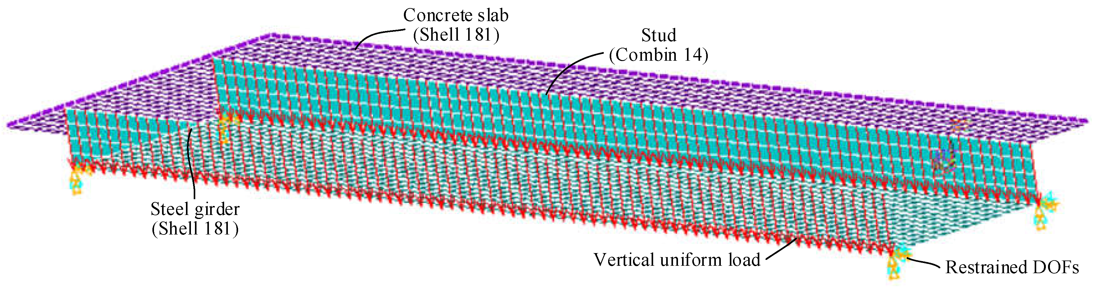
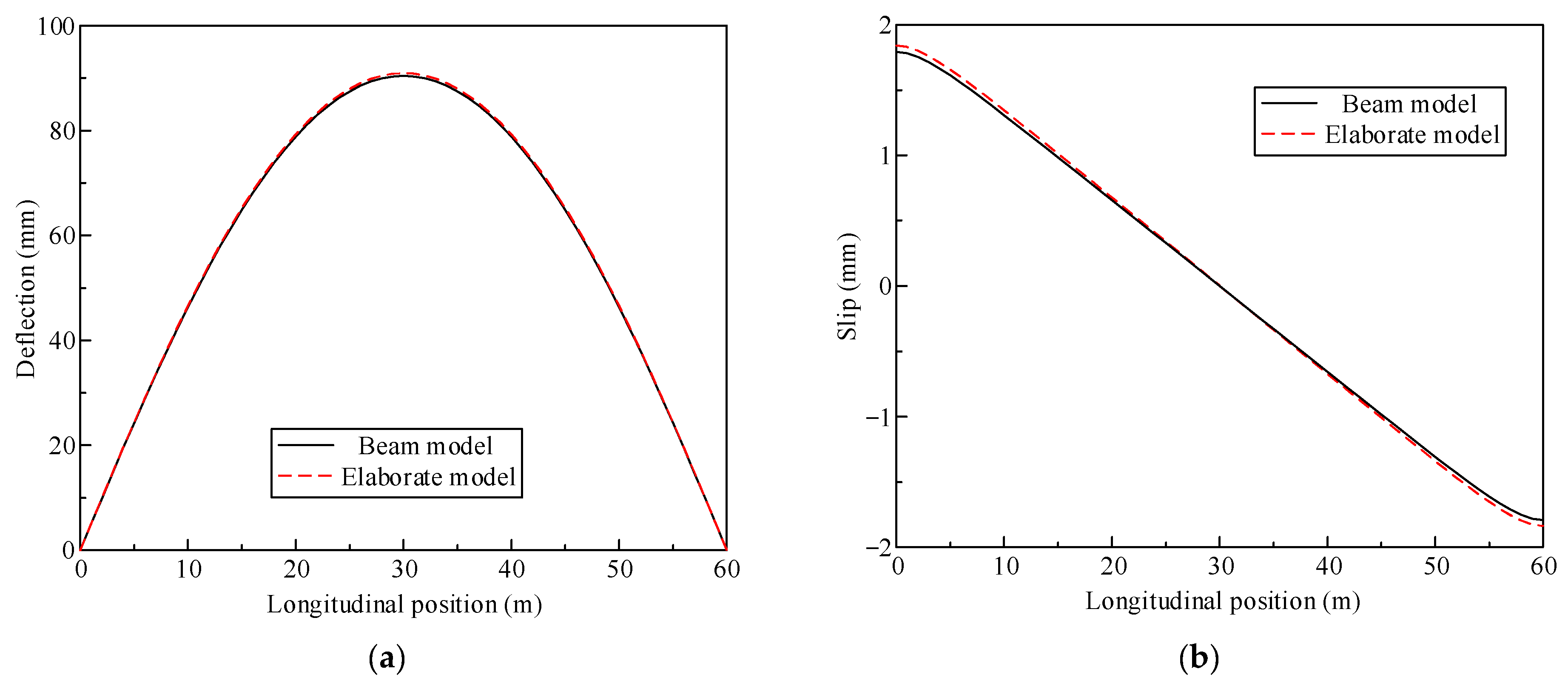
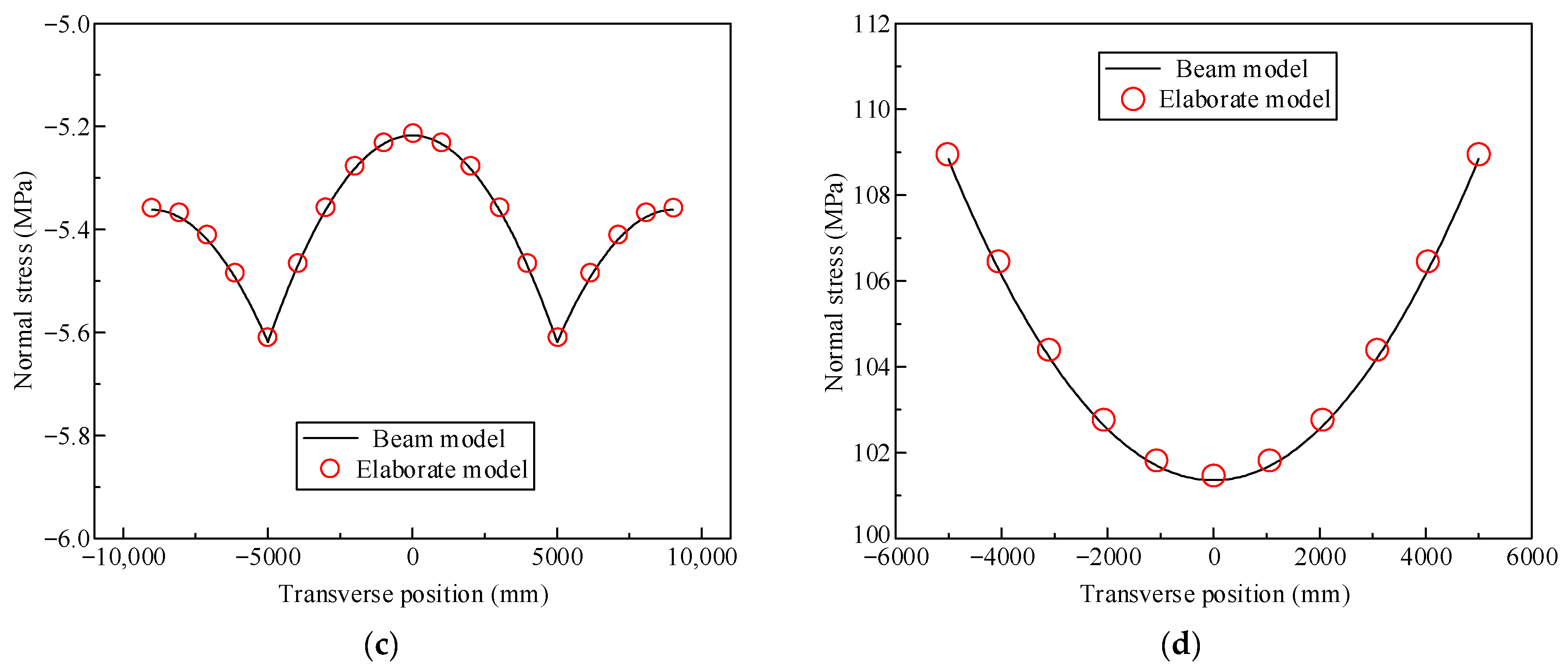
4.1. Instantaneous Behavior

First, the instantaneous behavior of a simply supported composite beam applied to a project under the action of a uniform load is analyzed. The standard span length of the composite beam is 60 m, and the parameters of the cross-section are illustrated in

Table 1. Cross-section of a simply supported composite beam (validation through instantaneous analysis).

bc (mm)	bc1 (mm)	tc (mm)	bs (mm)	bs1 (mm)	ts (mm)	bst (mm)	tst (mm)	hs (mm)	tw (mm)
9000	5000	300	5000	5000	24	600	16	3000	20

. The material properties of the specimen are listed as follows: shear connection stiffness ρ = 1 kN/mm², steel elastic modulus E_s = 2.06 × 10⁵ MPa, steel Poisson’s ratio μ_s = 0.3, concrete elastic modulus E_c = 3.8629 × 10⁴ MPa, and concrete Poisson’s ratio μ_c = 0.2. A vertical uniform load of 200 kN/m is applied to the simply supported composite beam.

The elaborate finite element (FE) model and the proposed finite beam element model of the simply supported composite beam were utilized to numerically analyze the structure. The elaborate FE model was established by using a commercial software, ANSYS version 18.0, as follows: both the concrete slab and steel beam were meshed by using shell elements (four-node general order Shell181 element in ANSYS). The studs at the interface between the steel plate and the concrete were simulated by using a linear spring element (two-node general order Combin14 element in ANSYS). The elastic stiffness of the shear studs was calculated as per CEB-FIP Model Code 1990 [37]. Figure 5 shows the elaborate FE model of the simply supported composite beam in ANSYS, which has 4860 nodes and 5612 elements. The mesh size of the elaborate element model is approximately 600 mm.

The beam element was established by using MATLAB 2019. A mesh sensitivity test was performed in which 20 beam elements and 21 nodes were used to mesh the specimens. The results showed that the sensitivity of the FE simulation results is within 1% of the observed values. The boundary conditions for the simply supported beam are listed in

Table 2. Boundary conditions for beam element model.

Location of Section	Restraint DOFs
Both ends of the beam	u, v, ϕ
Mid-span	wc, ws, fc, fs

. In order to ensure simulation of the boundary condition of the simply supported beam, the longitudinal displacements of concrete slab and steel girder w_c and w_s and the intensity functions of warping due to shear lag on concrete slab and steel girder f_c and f_s are restricted in the mid-span. The transverse displacement u, vertical displacement v, and torsion angle ϕ are restricted at both ends of the beam.

Figure 6 shows the calculation results of the elaborate FE model and proposed finite beam element model, including vertical deflections, interface slip, stresses on the concrete slab, and stresses at the bottom flange of the steel beam. The figure shows that the deviation between the two calculations is only within 5%.

In terms of the computation cost, the elaborate FE model requires 15.32 s, while the proposed beam element requires a total of 1.56 s. Therefore, the proposed beam element has notably higher computational efficiency than the elaborate FE model.

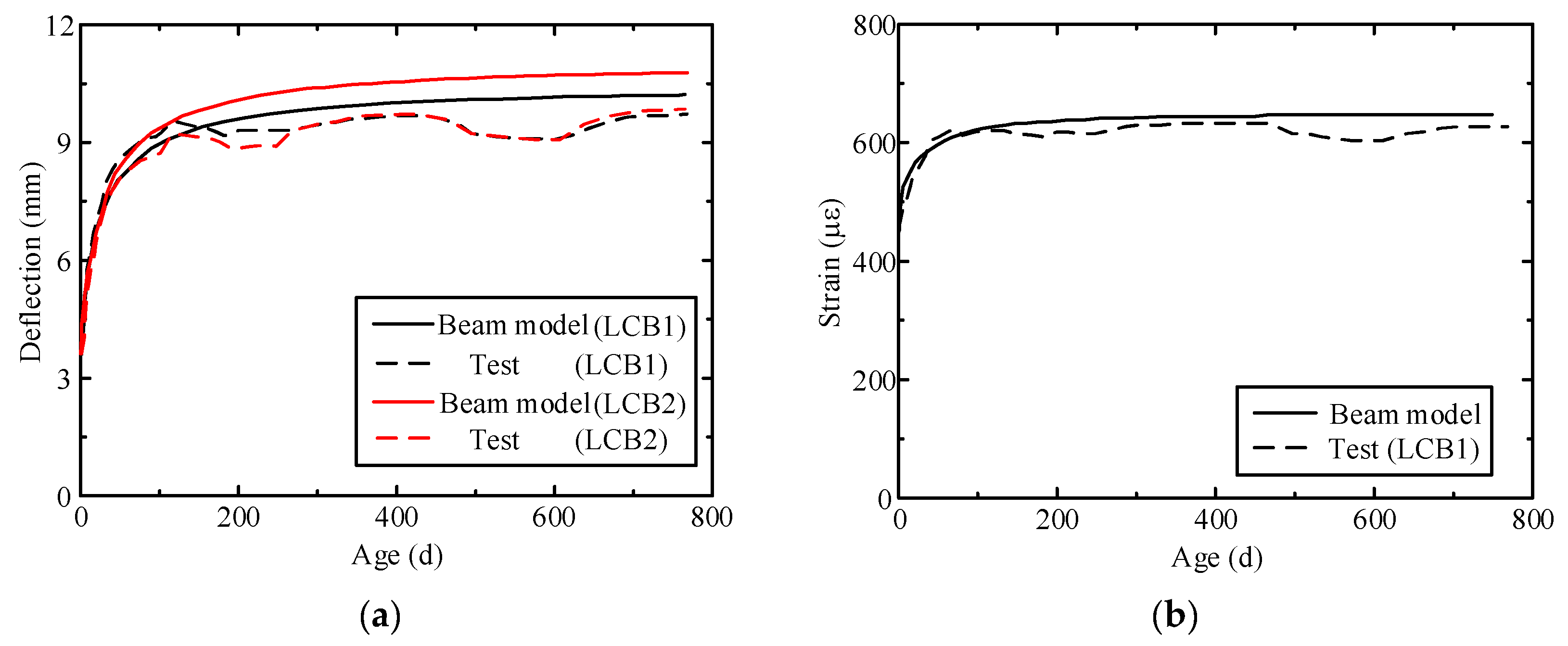
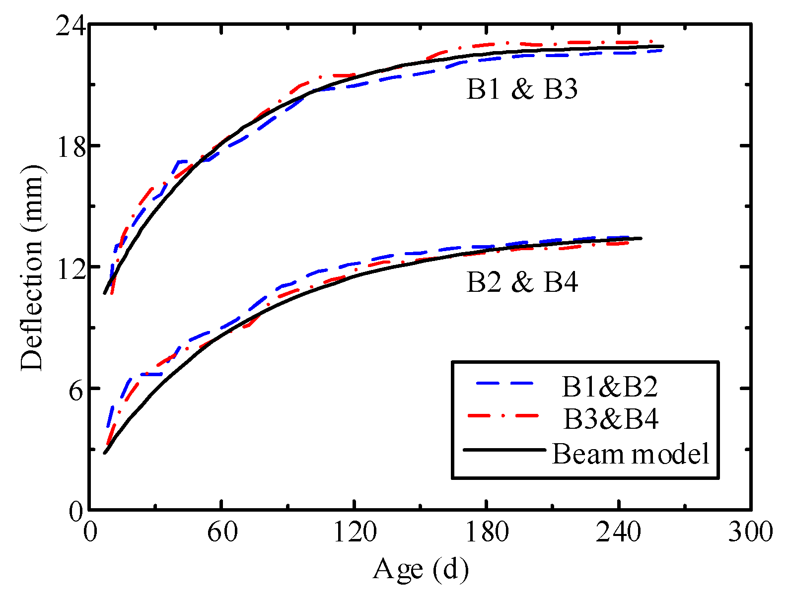
4.2. Time-Dependent Behavior

Fan et al. [38] carried out a test of two composite beams under vertical uniform loads in the long term. Both specimens have identical geometry configuration: the span of the composite box beam is 4 m, the steel beam height is 180 mm, the thickness of the reinforced concrete slab is 60 mm, and its width is 600 mm. A row of studs was welded on the upper flange of the steel beam with an interval of 80 mm longitudinally. The concrete slabs of specimens LCB1 and LCB2 were constructed of C20 concrete and C30 concrete, respectively. The cubic compressive strengths on the 7th day and the 28th day of the concrete applied in LCB1 were tested to be 24.3 MPa and 32.3 MPa, respectively. The cube compressive strengths on the 7th day and 28th day of the concrete applied in LCB2 were 33.4 MPa and 44.7 MPa, respectively. The composite beams were loaded from the 7th day of age continuously and constantly and had been monitored for 3 years. The vertical uniform load (including the weight of the beam itself) was 6.23 kN/m.

Figure 7 shows the test results and predicted results in comparison of the proposed finite beam element model, focusing on the vertical displacement of the composite beams and the strain development in the bottom flange of the steel beam. In the proposed model, the shrinkage strains measured in the material tests and the creep model referring to CEB-FIP 90 [37] are adopted to consider the shrinkage and creep of the concrete. The model results show agreement with the test results.

Bradford and Gilbert [39] conducted long-term performance tests on four simply supported steel–concrete composite beams with specimens named B1 to B4. Specimens B1 and B2 arrange two rows of studs with an interval 200 mm longitudinally. Specimens B3 and B4 arrange two rows of studs with an interval 600 mm longitudinally. The uniform vertical loads are sustained by the specimens B2 and B4 considering self-weight (1.92 kN/m) only, while those that are sustained by the specimens B1 and B3 consider self-weight (1.92 kN/m) and extra uniform loads (7.52 kN/m). The cylindrical compressive strength and elastic modulus of the concrete applied in the specimens is 31.1 MPa and 2.51 × 10⁴ MPa, respectively. The elastic modulus of steel is 2.0 × 10⁵ MPa, the final value of shrinkage of concrete on the 220th day was 410 × 10⁻⁶, and the coefficient of creep was 2.6.

Figure 8 displays the measured vertical displacements of the specimens and the predicted results of the proposed finite beam element model. As for the model, the coefficient curves of the shrinkage strain and creep coefficient of concrete are determined by the material tests. The prediction results of the proposed model show agreement with the test results.

A comparison between the experimental data given in [38,39] and the prediction model proposed by Zhu and Su [35] was carried out. The comparison results obtained by Zhu and Su are similar to those obtained by this study, as shown in Figure 7 and Figure 8.

5. Application of the Beam Finite Element Model

The proposed method is applied to predict the time-dependent behaviors of simply supported composite beams. The span of the composite beam is 40 m, the parameters of the cross-section shown in

Table 3. Cross-section of the composite bridge (application).

bc (mm)	bc1 (mm)	tc (mm)	bs (mm)	bs1 (mm)	ts (mm)	bst (mm)	tst (mm)	hs (mm)	tw (mm)
6500	4000	250	4000	4000	24	600	12	2000	16

. The material properties of the specimens are as follows: shear connection stiffness ρ = 1 kN/mm², elastic modulus of steel E_s = 2.06 × 10⁵ MPa, Poisson’s ratio of steel μ_s = 0.3, cubic compressive strength of concrete f_ck = 50 MPa, elastic modulus of concrete E_c = 3.8629 × 10⁴ MPa, and Poisson’s ratio of concrete μ_c = 0.2, the shrinkage age t_sh = 7 d, loading age t₀ = 28 d, and relative humidity RH = 75%. A vertical uniform load of 200 kN/m was applied to the composite beam. The shrinkage strain and creep coefficient calculation methods specified in CEB-FIP 90 [37] were adopted in the model.

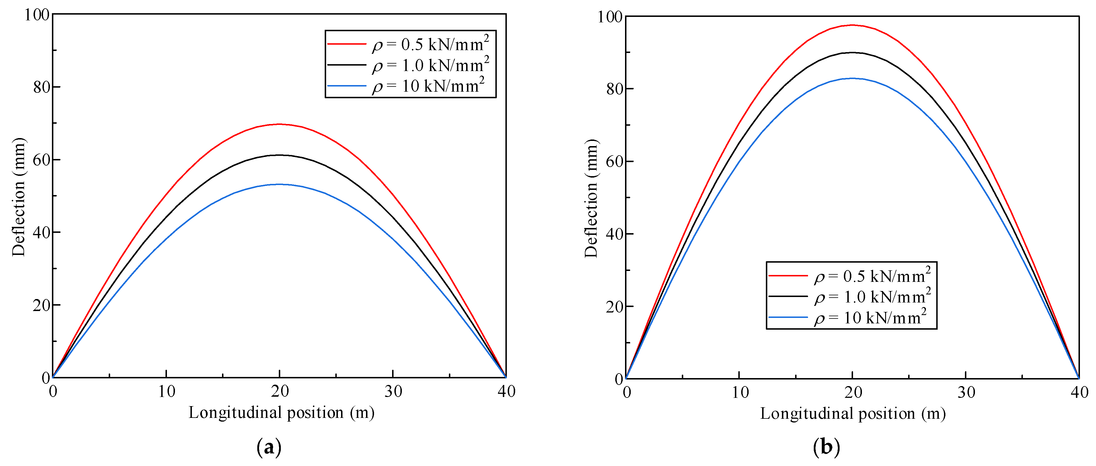
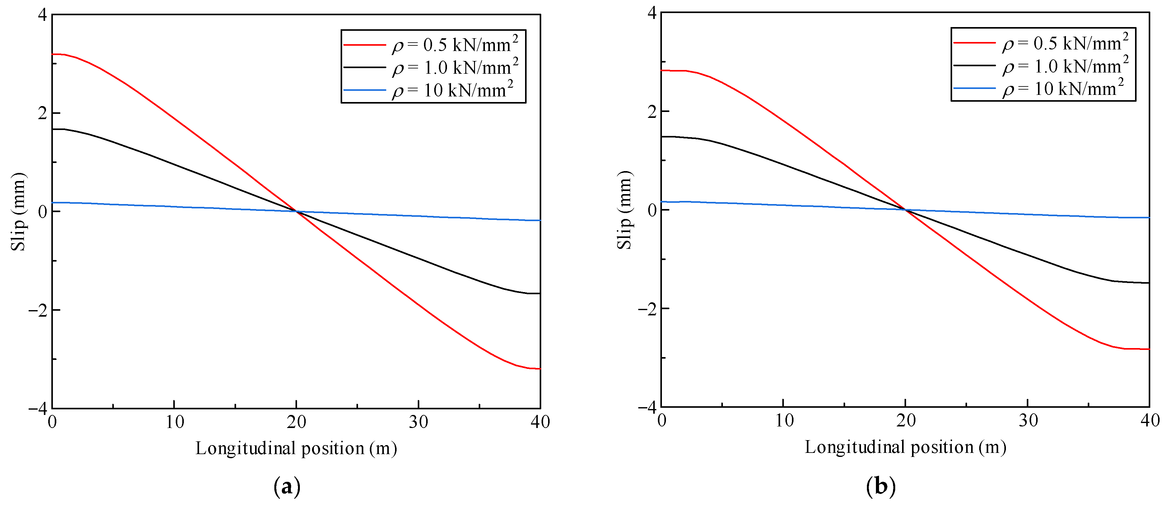
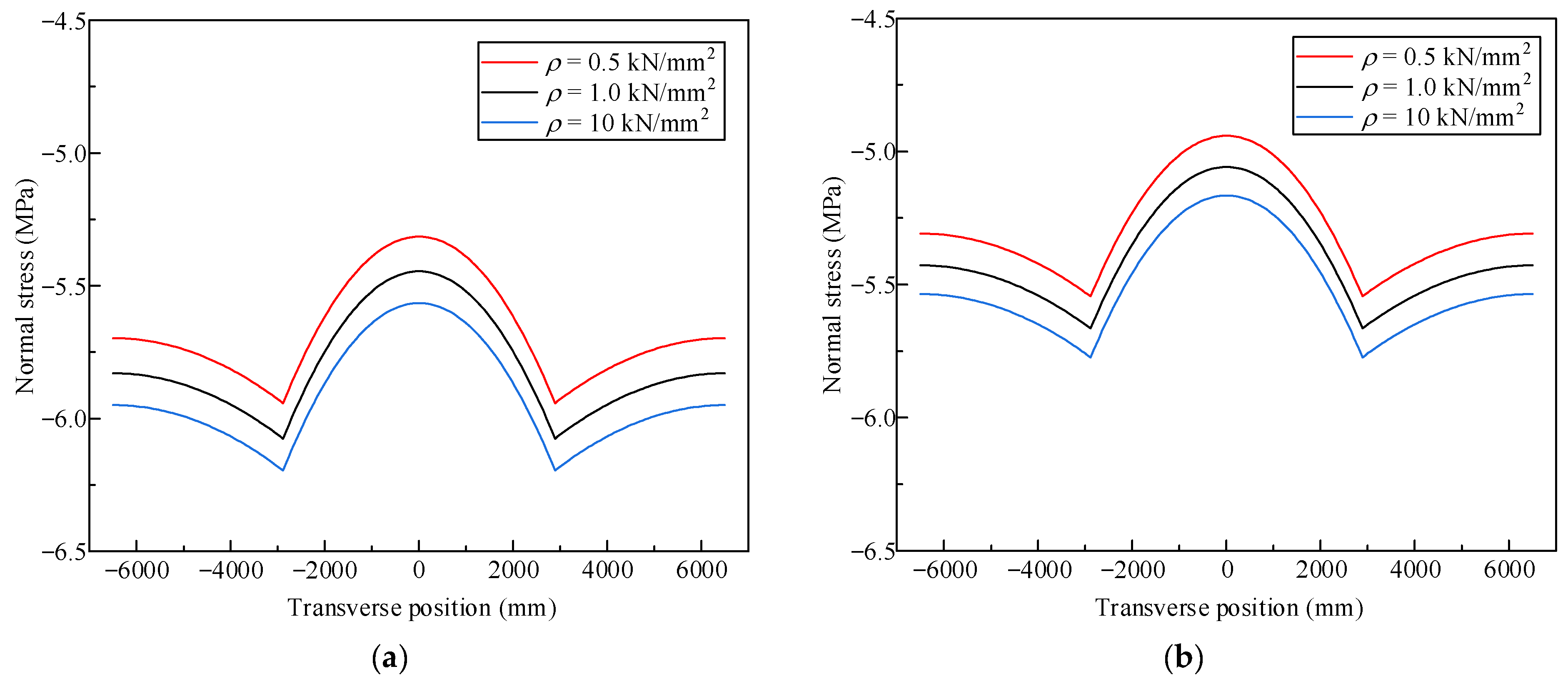
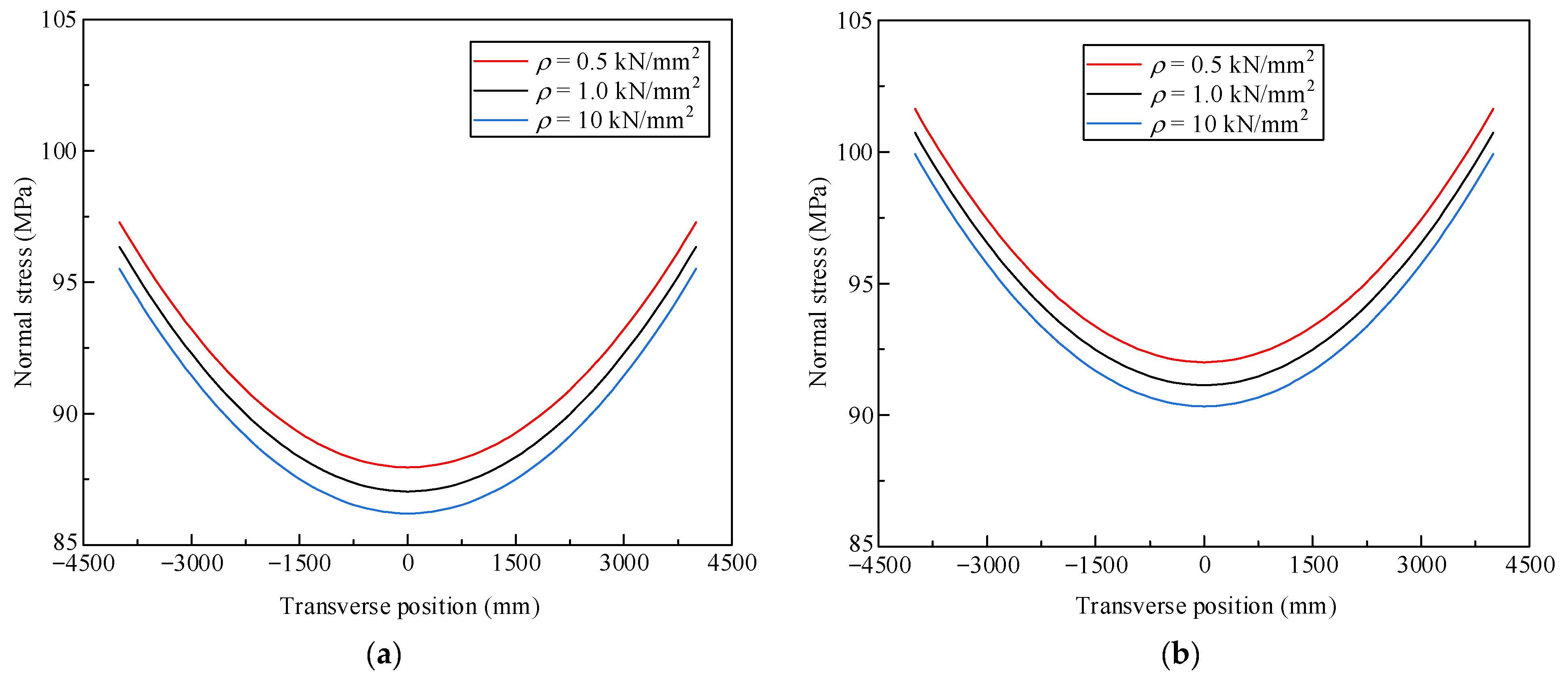
5.1. Influence of the Shear Connection Stiffness

To investigate the influence of shear connection stiffness, two other composite beam models with dissimilar shear connection stiffnesses were also analyzed for the cases ρ = 0.5 kN/mm² and ρ = 10 kN/mm². Figure 9, Figure 10, Figure 11 and Figure 12 show the vertical deflections, interface slip, the stresses of the concrete slab, and the bottom flange of the steel beam, where (a) and (b) represent the 28th day and 3rd year, respectively. According to the above figures, compared to the model with ρ = 1 kN/mm², the mid-span vertical deflections of the model with ρ = 0.5 kN/mm² on the 28th day and in the 3rd year are 13.90% larger and 8.40% larger, respectively; for the interface slip at the beam end, the vertical deflections are 91.64% larger and 90.62% larger, respectively; for the maximum compressive stress on the concrete slab, the vertical deflections are 2.2% smaller and 2.13% smaller, respectively; for the maximum tensile stress in the steel beam bottom flange, the vertical deflections are 1.06% larger and 0.96% larger, respectively. Compared to the model with ρ = 1 kN/mm², the mid-span vertical deflections of the model with ρ = 10 kN/mm² on the 28th day and in the 3rd year are 13.08% smaller and 7.90% smaller, respectively; for the interface slip at the support, the vertical deflections are 89.13% smaller and 89.20% smaller, respectively; for the maximum compressive stress on the concrete slab, the vertical deflections are 1.97% larger and 1.91% larger, respectively; for the maximum tensile stress in the steel beam bottom flange, the vertical deflections are 0.96% smaller and 0.88% smaller, respectively.

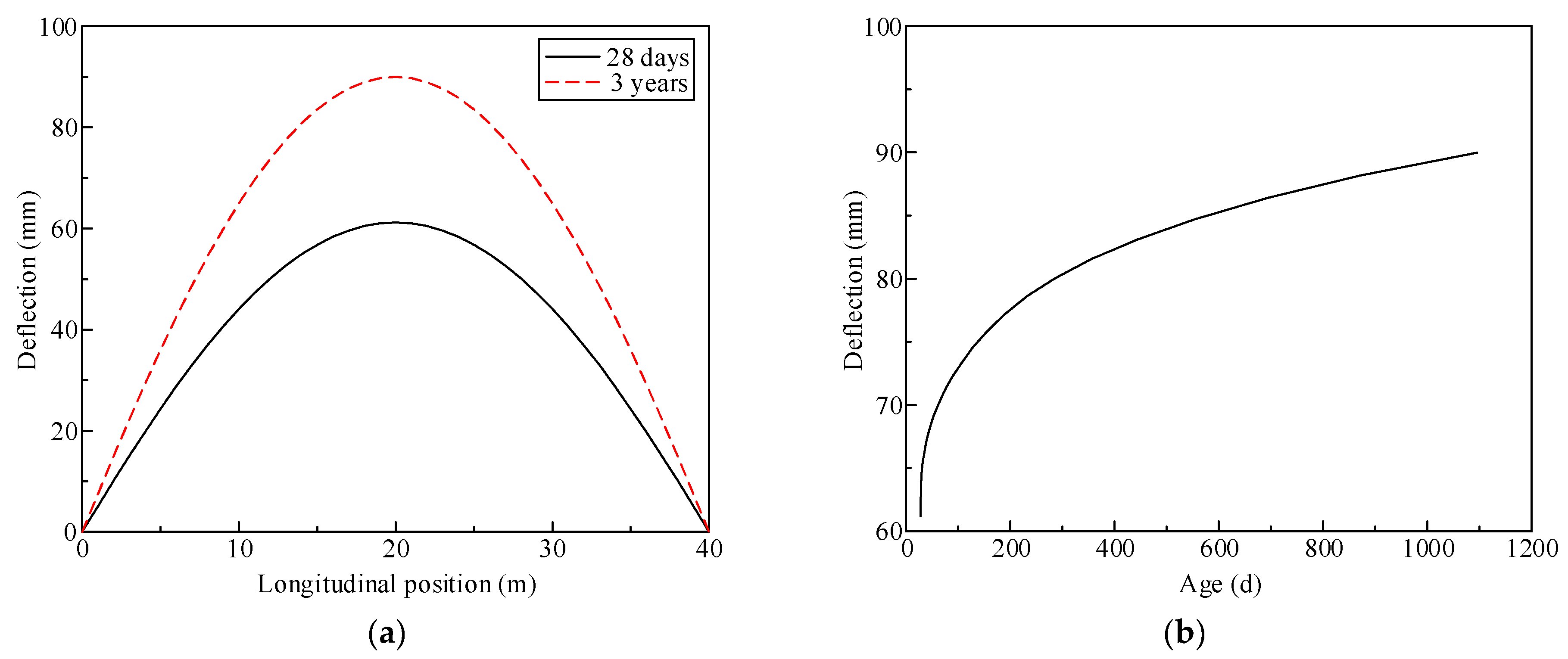
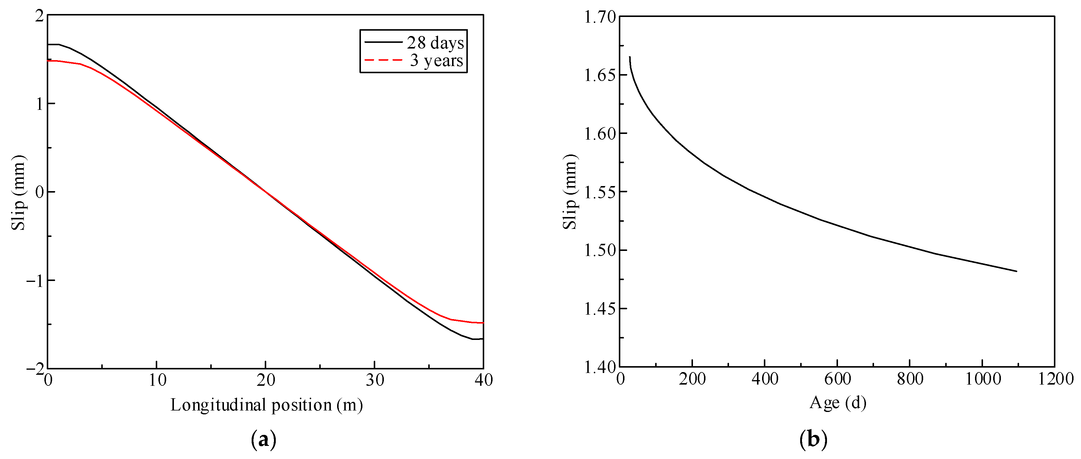
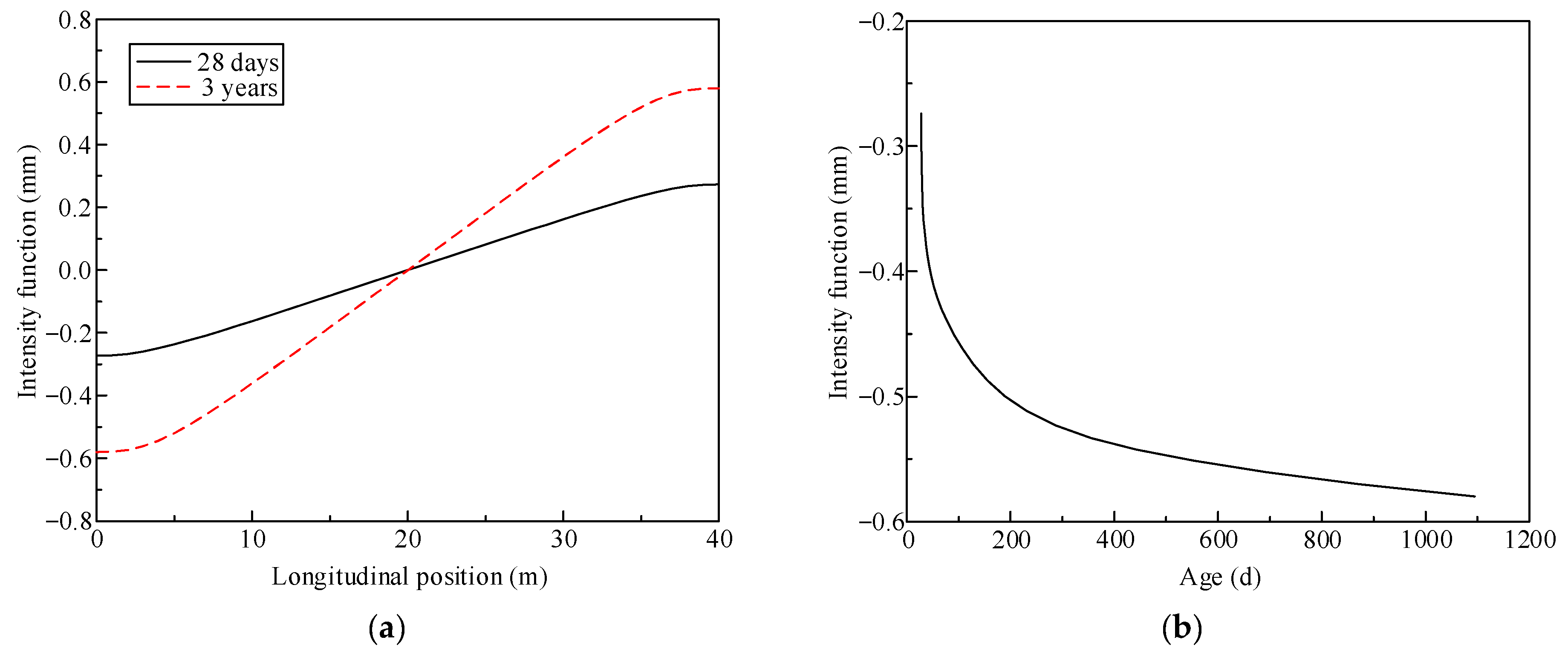
5.2. Time-Dependent Analysis

Time-dependent analysis of the above composite box beams focuses on the mechanical responses on the 28th day and in the 3rd year. Figure 13, Figure 14, Figure 15, Figure 16, Figure 17 and Figure 18 exhibit the time-dependent responses of the composite beams, including the vertical deflections, interface slip, warping intensity function on the concrete slab due to shear deformation, warping intensity function at the bottom flange of the steel beam due to shear deformation, and stresses on the concrete slab and at the bottom flange of steel beam, respectively. Figure 13a, Figure 14a, Figure 15a, Figure 16a, Figure 17a and Figure 18a show the distribution of these responses on the 28th day and in the 3rd year, while Figure 13b, Figure 14b, Figure 15b, Figure 16b, Figure 17b and Figure 18b show the changes over time.

Figure 13 shows the time-dependent variation in the vertical deflection of the composite beam. Figure 13a indicates that the long-term vertical deflection in the 3rd year is 47.01% larger than that on the 28th day. The time-dependent variation in the deflection at mid-span is shown in Figure 13b. It can be noted that the vertical deflection increases gradually over time, but in a narrower range.

Figure 14 shows the time-dependent interface slip between the concrete slab and the steel beam. This response is consistent with the common observation that obvious slip often occurs at the end of composite beams. The interface slip at the end of the composite beam continually decreases from 1.665 mm on the 28th day to 1.482 mm in the 3rd year, as illustrated in Figure 14a. Figure 14b shows the variation in the interface slip at the beam end. The interface slip gradually decreases over time, but in a narrower range.

Figure 15 shows the time-dependent variation in the shear lag warping intensity function of the concrete slab. Figure 15a shows that this response is more significant at the support of the composite beam, while this response is 0 at mid-span. This response in the 3rd year was 111.64% higher than that on the 28th day. Figure 15b exhibits the time-dependent variations in the warping intensity function of the concrete slab at the support of the composite beam. The warping intensity function of the concrete slab increases gradually over time, but in a narrow range. The increase slowed after the 400th day.

Figure 16 shows the time-dependent variations in the warping intensity function at the bottom flange of the steel beam due to shear deformation. As shown in Figure 16a, this response at the beam end in the 3rd year is 7.01% higher than that on the 28th day. Figure 16b shows the changes in the response at the composite beam end. The response at the support of the composite beam gradually increases over time, but in a narrower range. The increase in the warping intensity function of the concrete slab is more significant than that at the bottom flange of the steel beam.

Figure 17 shows the stress distribution on the concrete slab and the variation with time. According to Figure 17a, the compressive stress at the edge of the concrete slab decreases from 5.829 MPa on the 28th day to 5.428 MPa in the 3rd year; the compressive stress at the intersection between the steel web and the concrete slab decreased from 6.075 MPa on the 28th day to 5.665 MPa in the 3rd year; the compressive stress of the centerline of the concrete slab decreases from 5.446 MPa on the 28th day to 5.058 MPa in the 3rd year. Figure 17b shows the variation in these stresses with time and reveals that the stress on the concrete slab slowly decreases after the 400th day.

Figure 18 exhibits the stress distribution of the bottom flange of the steel beam and the change over time. Figure 18a shows that the stress at the steel web–concrete slab intersection increases from 96.349 MPa on the 28th day to 100.739 MPa in the 3rd year; the stress of the centerline of the steel bottom increases from 87.039 MPa on the 28th day to 91.133 MPa in the 3rd year. Figure 18b shows the variation in these stresses with time and reveals that the stress of steel slowly increases after the 400th day.

To better show the time-dependent influence, the composite beam on the 3650th day was analyzed. Figure 19 shows the stress distribution on the concrete slab on the 28th and 3650th days. Figure 20 shows the stress distribution at the steel bottom on the 28th and 3650th days. The stress on the concrete slab decreases over this period (28th to 3650th day), and the stress at the bottom flange of the steel beam increases. These results indicate that the creep of concrete produces an unloading effect on the concrete slab.

6. Conclusions

A beam finite element model with 18 DOFs considering slip, shear lag, and time-dependent effects of the composite box beam is proposed in this study. The conclusions from the numerical results are drawn as follows:

(1)

The analytical model of the composite box beam is solved in the time domain by an accurate step-by-step method, and the Dirichlet series is employed into the creep function without the storage of stress and strain histories. In the spatial domain, the FEM discretizes the composite beam into finite two-node beam elements with 18 DOFs. An effective recursion method was developed to solve these equations of the system.

(2)

A fine numerical simulation by ANSYS is performed to validate the correctness and applicability of the proposed model in instantaneous analysis. Through a comparison between the classical long-term test results of the composite beams and the calculation results of the proposed model involving beam finite elements, the validity and applicability of the proposed model used in the long-term analysis was proven.

(3)

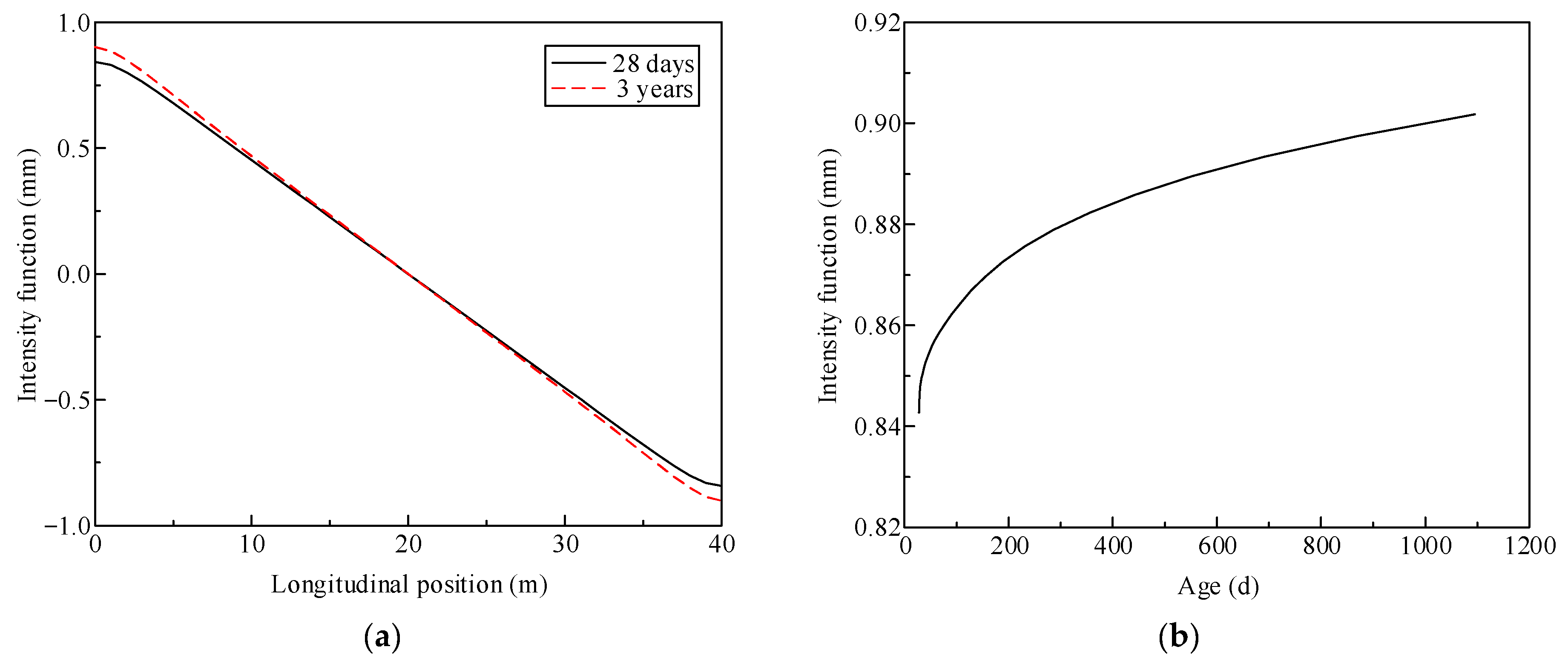
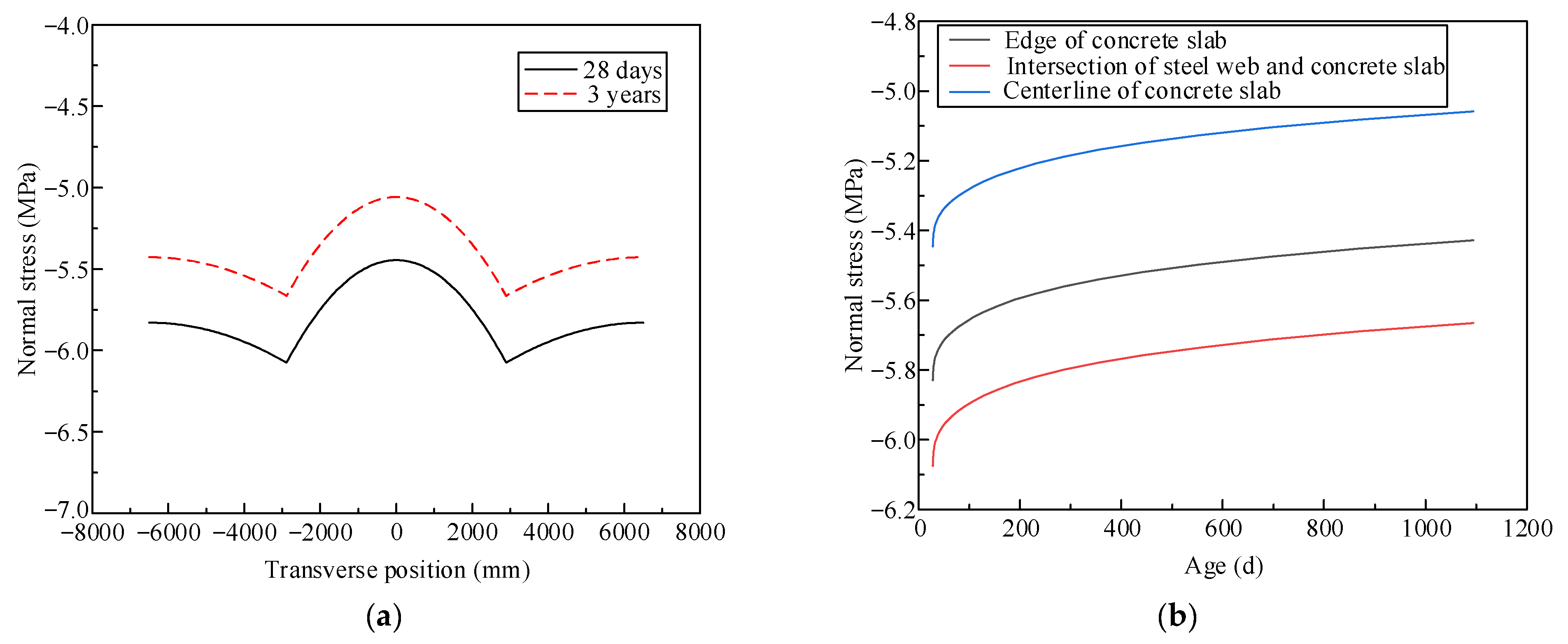
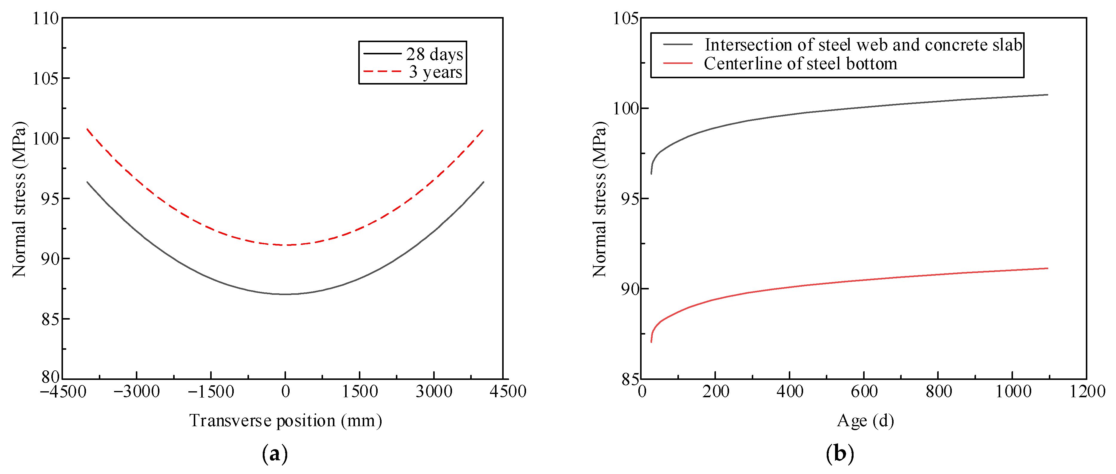
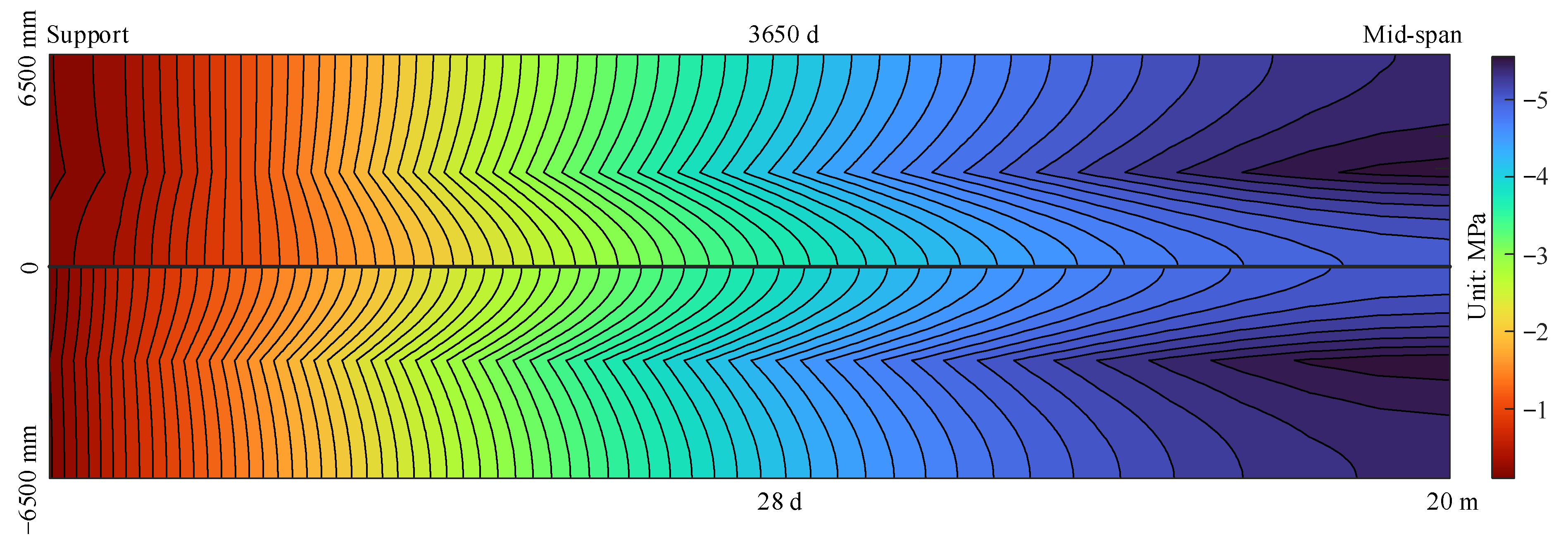
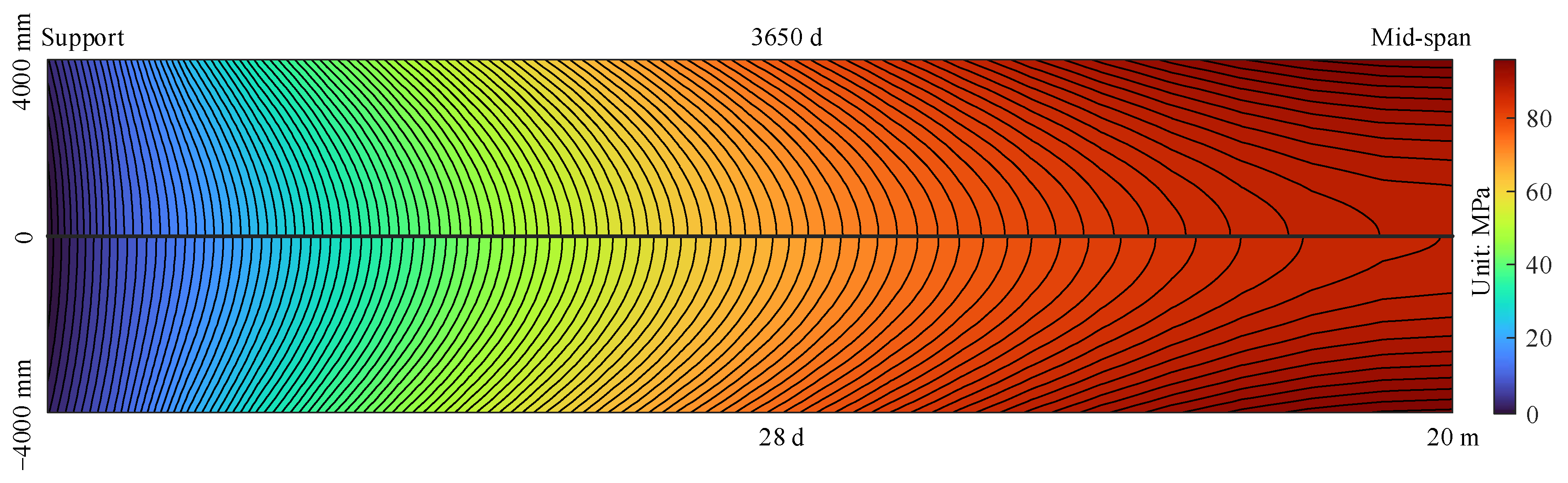
The proposed model is then applied to the analysis of the time-dependent behavior of composite beams. Some mechanical responses, including vertical deflections, interface slip, warping intensity function due to shear deformation, the stress on the concrete slab, and the stress of the steel beam, are analyzed. In this study, the variation in these responses between the 28th day and the 3rd year was the focus. It was determined that the shear connection stiffness, shrinkage, and creep all have a significant impact on these responses.

(4)

Compared with the model with ρ = 1 kN/mm², the vertical deflection at mid-span in the 3rd year of the model with ρ = 0.5 kN/mm² is 8.40% larger; the interface slip at the end is 90.62% larger; the mid-span vertical deflection in the 3rd year of the model with ρ = 10 kN/mm² is 7.90% less; and the interface slip at the end is 89.20% smaller.

(5)

For the model with ρ = 1 kN/mm², from the 28th day to the 3rd year, the mid-span vertical deflection increased by 47.01%, the interface slip at the end decreased by 10.99%, the warping intensity function of the concrete slab at end of the steel beam due to shear deformation increased by 111.64%, the warping intensity function at the steel bottom near the beam end increased by 7.01%, the maximum compressive stress on the concrete slab decreased by 6.75%, and the maximum tensile stress at the steel bottom flange increased by 4.56%. The above mechanical responses have been developing, and even in the 10th year, the development rate is still not negligible.

References

1. Doori, S.G.; Noori, A.R. Finite element approach for the bending analysis of castellated steel beams with various web openings. ALKU J. Sci. 2021, 3, 38–49. [Google Scholar] [CrossRef]
2. Jiang, L.Z.; Nie, L.X.; Zhou, W.B.; Wu, X.; Liu, L.L. Distortional buckling analysis of steel–concrete composite box beams considering effect of stud rotational restraint under hogging moment. J. Cent. South Univ. 2022, 29, 3158–3170. [Google Scholar] [CrossRef]
3. Shen, J.; Pagani, A.; Arruda, M.R.T.; Carrera, E. Exact component-wise solutions for 3D free vibration and stress analysis of hybrid steel–concrete composite beams. Thin-Walled Struct. 2022, 174, 109094. [Google Scholar] [CrossRef]
4. Lou, T.; Wu, S.; Chen, B. Effect of reinforcement on the response of continuous steel–concrete composite beams. Case Stud. Constr. Mater. 2022, 16, e00929. [Google Scholar] [CrossRef]
5. Fan, J.S.; Li, B.L.; Liu, C.; Liu, Y.F. An efficient model for simulation of temperature field of steel–concrete composite beam bridges. Structures 2022, 43, 1868–1880. [Google Scholar] [CrossRef]
6. Chisari, C.; Amadio, C. An experimental, numerical and analytical study of hybrid RC-encased steel joist beams subjected to shear. Eng. Struct. 2014, 61, 84–98. [Google Scholar] [CrossRef]
7. Colajanni, P.; Mendola, L.L.; Monaco, A. Experimental investigation of the shear response of precast steel–concrete trussed beams. J. Struct. Eng. ASCE 2017, 143, 04016156. [Google Scholar] [CrossRef]
8. Foutch, D.A.; Chang, P.C. A shear lag anomaly. J. Struct. Eng. ASCE 1982, 108, 1653–1658. [Google Scholar] [CrossRef]
9. Chang, S.T.; Fang, Z.Z. Negative shear lag in cantilever box girder with constant depth. J. Struct. Eng. ASCE 1987, 113, 20–35. [Google Scholar] [CrossRef]
10. Kristek, V.; Studnicka, J. Discussion of ‘negative shear lag in cantilever box girder with constant depth’. J. Struct. Eng. ASCE 1988, 114, 2168–2173. [Google Scholar]
11. Chang, S.T.; Ding, Y. Shear lag effect in box girder with varying depth. J. Struct. Eng. ASCE 1988, 114, 2280–2292. [Google Scholar] [CrossRef]
12. Cao, G.H.; Han, C.C.; Dai, Y.; Zhang, W. Long-term experimental study on prestressed steel–concrete composite continuous box beams. J. Bridge Eng. ASCE 2018, 23, 04018067. [Google Scholar] [CrossRef]
13. Huang, D.; Wei, J.; Liu, X.; Xiang, P.; Zhang, S. Experimental study on long-term performance of steel–concrete composite bridge with an assembled concrete deck. Constr. Build. Mater. 2019, 214, 606–618. [Google Scholar] [CrossRef]
14. Huang, D.; Wei, J.; Peng, H.; Guo, H.L.; Wang, B.W. An analysis model accounting for time-dependent shear lag effects in assembled composite bridge decks. Adv. Struct. Eng. 2022, 25, 1866–1877. [Google Scholar] [CrossRef]
15. Souici, A.; Tehami, M.; Rahal, N.; Bekkouche, M.S.; Berthet, J.F. Creep effect on composite beam with perfect steel–concrete connection. Int. J. Steel Struct. 2015, 15, 433–445. [Google Scholar] [CrossRef]
16. Henriques, D.; Gonçalves, R.; Sousa, C.; Camotim, D. GBT-based time-dependent analysis of steel–concrete composite beams including shear lag and concrete cracking effects. Thin-Walled Struct. 2020, 150, 106706. [Google Scholar] [CrossRef]
17. Dezi, L.; Gara, F.; Leoni, G.; Tarantino, A.M. Time dependent analysis of shear-lag effect in composite beams. J. Eng. Mech. ASCE 2001, 127, 71–79. [Google Scholar] [CrossRef]
18. Dezi, L.; Leoni, G. Effective slab width in prestressed twin-girder composite decks. J. Struct. Eng. ASCE 2006, 132, 1358–1370. [Google Scholar] [CrossRef]
19. Dezi, L.; Gara, F.; Leoni, G. Shear-lag effect in twin-girder composite decks. Steel Compos. Struct. 2003, 3, 111–122. [Google Scholar] [CrossRef]
20. Gara, F.; Leoni, G.; Dezi, L. A beam finite element including shear lag effect for the time-dependent analysis of steel–concrete composite decks. Eng. Struct. 2009, 31, 1888–1902. [Google Scholar] [CrossRef]
21. Gara, F.; Ranzi, G.; Leoni, G. Short- and long-term analytical solutions for composite beams with partial interaction and shear-lag effects. Int. J. Steel Struct. 2010, 10, 359–372. [Google Scholar] [CrossRef]
22. Madenci, E.; Ozkilic, Y.O.; Gemi, L. Buckling and free vibration analyses of pultruded GFRP laminated composites: Experimental, numerical and analytical investigations. Compos. Struct. 2020, 254, 112806. [Google Scholar] [CrossRef]
23. Madenci, E.; Ozkilic, Y.O.; Gemi, L. Experimental and theoretical investigation on flexure performance of pultruded GFRP composite beams with damage analyses. Compos. Struct. 2020, 242, 112162. [Google Scholar] [CrossRef]
24. Gemi, L.; Madenci, E.; Ozkılıc, Y.O. Experimental, analytical and numerical investigation of pultruded GFRP composite beams infilled with hybrid FRP reinforced concrete. Eng. Struct. 2021, 244, 112790. [Google Scholar] [CrossRef]
25. Madenci, E.; Ozkilic, Y.O. Free vibration analysis of open-cell FG porous beams: Analytical, numerical and ANN approaches. Steel Compos. Struct. 2021, 40, 157–173. [Google Scholar]
26. The International Federation for Structural Concrete. CEB Design Manual on Structural Effects of Time Dependent Behavior of Concrete; CEB Bulletin D’Information: Saint-Saphorin, Switzerland, 1984. [Google Scholar]
27. Bazant, Z.P.; Baweja, S. Creep and shrinkage prediction model for analysis and design of concrete structures: Model B3. In Adam Neville Symposium: Creep and Shrinkage-Structural Design Effects, Proceedings of the Adam Neville Symposium, Atlanta, GA, USA, November 1997; American Concrete Institute: Farmington Hills, MI, USA, 2000; pp. 1–83. [Google Scholar]
28. Bazant, Z.P. Prediction of concrete creep effects using age-adjusted effective modulus method. ACI J. 1972, 69, 212–217. [Google Scholar]
29. Zhang, H.; Quan, L.W.; Wang, L.; Wu, J.X.; Zhang, Z.C. Analyses on long-term behavior of composite steel–concrete beams with weak interface using a state space approach. Eng. Struct. 2021, 231, 111781. [Google Scholar] [CrossRef]
30. Bazant, Z.P. Numerical determination of long-range stress history from strain history in concrete. Mater. Struct. 1972, 5, 135–141. [Google Scholar]
31. Bazant, Z.P.; Wu, S.T. Rate-type creep law of aging concrete based on Maxwell chain. Mater. Struct. 1974, 7, 45–60. [Google Scholar]
32. Bazant, Z.P.; Asghari, A. Computation of age-dependent relaxation spectra. Cem. Concr. Res. 1974, 4, 567–579. [Google Scholar] [CrossRef]
33. Bazant, Z.P.; Kim, S.S. Approximate relaxation function for concrete. J. Struct. Div. ASCE 1979, 105, 2695–2705. [Google Scholar] [CrossRef]
34. Bazant, Z.P. Mathematical Modeling of Creep and Shrinkage of Concrete; Wiley: Hoboken, NJ, USA, 1988. [Google Scholar]
35. Zhu, L.; Su, R.K.L. Analytical solutions for composite beams with slip, shear-lag and time-dependent effects. Eng. Struct. 2017, 152, 559–578. [Google Scholar] [CrossRef]
36. Zhu, L.; Zhao, G.Y.; Su, R.K.L.; Liu, W.; Wang, G.M. Time-dependent creep and shrinkage analysis of curved steel–concrete composite box beams. Mech. Adv. Mater. Struct. 2021. [Google Scholar] [CrossRef]
37. Comite Euro-International du Beton-Federation International de la Precontrainte (CEB-FIP). CEB-FIP Model Code 1990: Design Code; Thomas Telford, Ltd.: London, UK, 1993. [Google Scholar]
38. Fan, J.S.; Nie, J.G.; Li, Q.; Wang, H. Long-term behavior of composite beams under positive and negative bending. I: Experimental study. J. Struct. Eng. ASCE 2009, 136, 849–857. [Google Scholar] [CrossRef]
39. Bradford, M.A.; Gilbert, R.I. Time-dependent behaviour of simply-supported steel–concrete composite beams. Mag. Concr. Res. 1991, 43, 265–274. [Google Scholar] [CrossRef]
Figure 1. Shear lag and interface slip of a steel–concrete composite box beam.
Buildings 13 00215 g001
Figure 2. Geometric notation of composite beams. (a) Three-dimension; (b) Cross-section.
Buildings 13 00215 g002
Figure 3. Synoptic scheme of inputted geometric and mechanical parameters.
Buildings 13 00215 g003
Figure 4. Flow of the solution procedure.
Buildings 13 00215 g004
Figure 5. Finite elaborate element model of a simply supported composite bridge.
Buildings 13 00215 g005
Figure 6. Comparison of prediction results from the finite beam element and finite elaborate element models for a simply supported composite bridge. (a) Deflection; (b) Interface slip; (c) Normal stress of concrete slab at mid-span section; (d) Normal stress of steel flange at mid-span section.
Buildings 13 00215 g006aBuildings 13 00215 g006b
Figure 7. Comparison of the experimental results in [38] and the results of prediction for the finite beam element model. (a) Vertical deflection; (b) Normal strain of steel bottom flange (Adapted with permission from Ref. [35]. Copyright 2017 Elsevier.).
Buildings 13 00215 g007
Figure 8. The experimental results in [39] and the prediction results of the finite beam element model (Adapted with permission from Ref. [35]. Copyright 2017 Elsevier.).
Buildings 13 00215 g008
Figure 9. Vertical deflections of composite beams (influence of shear connection stiffness). (a) 28 days; (b) 3 years.
Buildings 13 00215 g009
Figure 10. Interface slip of composite beams (influence of shear connection stiffness). (a) 28 days; (b) 3 years.
Buildings 13 00215 g010
Figure 11. Stress on the concrete slab of composite beams (influence of shear connection stiffness). (a) 28 days; (b) 3 years.
Buildings 13 00215 g011
Figure 12. Stresses at the bottom flange of the steel beam (influence of shear connection stiffness). (a) 28 days; (b) 3 years.
Buildings 13 00215 g012
Figure 13. Deflection of the composite beam (time-dependent analysis). (a) Distribution along span; (b) Change with time at mid-span section.
Buildings 13 00215 g013
Figure 14. Interface slip of the composite beam (time-dependent analysis). (a) Distribution along span; (b) Change with time at support section.
Buildings 13 00215 g014
Figure 15. Warping intensity function of the concrete slab due to shear deformation of the composite beam (time-dependent analysis). (a) Distribution along span; (b) Change with time at support section.
Buildings 13 00215 g015
Figure 16. Warping intensity function of the steel bottom induced by shear deformation of the composite beam (time-dependent analysis). (a) Distribution along span; (b) Change with time at support section.
Buildings 13 00215 g016
Figure 17. Stress on the concrete slab of the composite beam (time-dependent analysis). (a) Distribution along width; (b) Change with time at mid-span section.
Buildings 13 00215 g017
Figure 18. Stress at the bottom flange of the steel beam of the composite beam (time-dependent analysis). (a) Distribution along width; (b) Change with time at mid-span section.
Buildings 13 00215 g018
Figure 19. Contour plot of stresses on the concrete slab of the composite beam.
Buildings 13 00215 g019
Figure 20. Contour plot of stresses at the bottom flange of the steel beam of the composite beam.
Buildings 13 00215 g020