Regression Models for Predicting the Global Warming Potential of Thermal Insulation Materials

Abstract

The impacts and benefits of thermal insulations on saving operational energy have been widely investigated and well-documented. Recently, many studies have shifted their focus to comparing the environmental impacts and CO₂ emission-related policies of these materials, which are mostly the Embodied Energy (EE) and Global Warming Potential (GWP). In this paper, machine learning techniques were used to analyse the untapped aspect of these environmental impacts. A collection of over 120 datasets from reliable open-source databases including Okobaudat and Ecoinvent, as well as from the scientific literature containing data from the Environmental Product Declarations (EPD), was compiled and analysed. Comparisons of Multiple Linear Regression (MLR), Support Vector Regression (SVR), Least Absolute Shrinkage and Selection Operator (LASSO) regression, and Extreme Gradient Boosting (XGBoost) regression methods were completed for the prediction task. The experimental results revealed that MLR, SVR, and LASSO methods outperformed the XGBoost method according to both the K-Fold and Monte-Carlo cross-validation techniques. MLR, SVR, and LASSO achieved 0.85/0.73, 0.82/0.72, and 0.85/0.71 scores according to the R² measure for the Monte-Carlo/K-Fold cross-validations, respectively, and the XGBoost overfitted the training set, showing it to be less reliable for this task. Overall, the results of this task will contribute to the selection of effective yet low-energy-intensive thermal insulation, thus mitigating environmental impacts.

1. Introduction

One of the most important and pressing needs of the future is key attention to decision-making policies on the interplay between climate and energy. Materials produced from where insulations are manufactured cause a significant adverse effect on the environment due to being commonly from petrochemicals and energy-intensive phases [1]. The United Nations Environment Programme estimated that buildings are responsible for about one-third of the GHG emissions worldwide and consume 40% of the world’s global energy and resources [2,3,4]. Mitigation attempts to reduce demand are focused on both user behaviours and enhancing insulation properties [5,6,7,8]. Thus, insulation materials should be produced in the most possible energy-efficient and sustainable ways. The emergence of the concept of sustainability in the building sector gave rise to the production of insulation products made from natural or recycled materials. Some of these insulation products are already present in the market while others are at the early stage of production [1]. Today, low-energy buildings and passive houses are undoubtedly the reference for many building designers and are known for their reduced energy requirements and high envelope insulation levels [9].

The role of thermal insulations for low-energy buildings cannot be overemphasised. However, their well-known embodied components, i.e., the GWP, cannot be overlooked. While new constructions are characterised by reduced operational energy consumption, plenty of attention should be given to the embodied components such as the GWP and Embodied Energy (EE) due to building materials and systems [1,10]. The EE impacts are rooted in the environmental processes of exploiting raw materials and how the raw materials are processed, manufactured, transported to a site, and constructed throughout their whole life cycle [9]. The degree of these EE impacts has further relevance to the performance of energy-efficient buildings [11,12,13]. Using the Life Cycle Assessment (LCA) methodology, some authors showed that high-level thermal insulation in buildings contributes significantly to the EE and GWP of the buildings [14].

Indeed, a measure of the differences in the environmental burden from EE in insulation materials and their operational energy savings during their use stage is necessary for their preferential selection. The choice for the application of building insulation materials can be expressed as the ratio between their embodied burdens and the total amount of impacts saved per year of the useful life of the material [9]. However, Biswas et al. [15] demonstrated that operational savings dominate embodied burdens, especially for low-thickness insulation materials. Whichever way, however, the evidence above shows the adverse impacts of EE associated with thermal insulations on the environment. Regardless of the degree of such impacts, there is a necessity for continuous studies not only on the operational savings but also on the degree of the embodied impacts of thermal insulation materials.

Due to the wide availability of thermal insulation materials and their thermal properties, accurate prediction models are important in order to have a deep understanding of their GWP. While predictive models intend to aid and accelerate the design process by bypassing many time-consuming experiments, they are not meant to replace these experimental methods. In fact, the foundation of predictive modelling is good-quality data that come from experimental studies only [16]. Few studies have used machine learning (ML) algorithms to predict the thermal properties (conductivity) of the most commonly used construction materials. Sargam et al. [16] developed a supervised ML prediction model for the thermal conductivity of concretes; Valipour and Bahramian [17] applied ML algorithms for predicting the thermal conductivity coefficient of polymeric aerogels and compared them with their real values for validation. However, to the best of our knowledge, no study has demonstrated how a machine learning algorithm can be used for predicting the future GWP in both natural and synthetic building thermal insulation materials. Therefore, the aim of this paper is to develop a robust ML model that can predict the GWP of building thermal insulation materials using a comparison of the different machine learning regression algorithms. In this paper, particular attention is given to relevant studies on LCA to develop a comprehensive dataset of thermal insulation materials, most especially those described in [9], considering their extractions from reputable databases, i.e., the EPD.

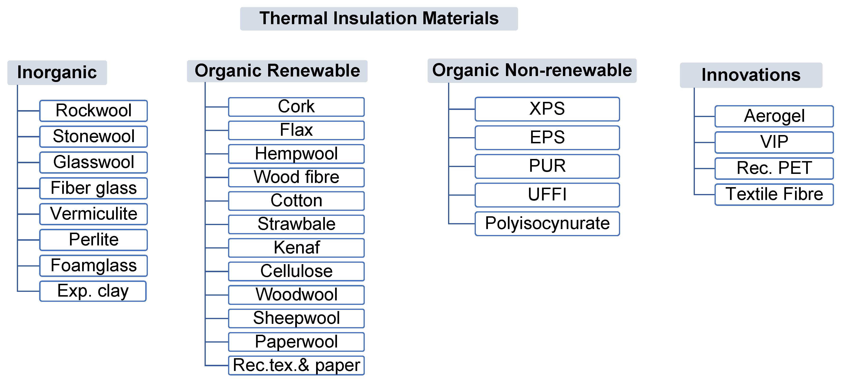
2. LCA of Building Thermal Insulation Materials

The Life Cycle Assessment (LCA) is a system analysis tool used for evaluating the environmental impact of a product or a process over its entire life cycle, from raw material acquisition to end-of-life [18,19]. It aims to comprehensively evaluate the resources used and the potential environmental impacts of each stage in the life cycle in a way that not only focuses on just one issue, such as climate change, but that covers a wide range of potential impacts [20]. With regard to materials, the objective of LCA studies is often to support decisions for more environmentally friendly materials or to identify environmentally crucial points in the production of building materials [21]. In this section, we highlight why these environmentally crucial points are necessary, i.e., those leading to embodied components within the cycle stages of thermal insulation materials, cutting across inorganic, organic renewable, organic non-renewable, and innovation technologies (Figure 1), which are discussed as extracted from the scientific literature. This aided in understanding the knowledge gap and in developing the datasets for the insulation materials in this study.

For inorganic materials, the energy-intensive melting and fiberizing process of glass [22,23] and rock materials [22] in the production phase is the most impactful. However, Bribian et al. [24] note that binders and additives could also have a high impact. For core organic non-renewable materials, EPS, XPS, and PUR have similar environmental crucial points, with raw materials constituting the highest impacts [15,24,25]. About 40–50% of the non-renewable energy required for EPS and PUR can be attributed to raw materials [26], while 90% of the GWP in EPS arises from raw materials [27]. For cellulose, the raw material played a role in the environmental impact, as cellulose insulation is typically made from recycled paper [22,28]. The use of additives such as fire retardant and anti-fungal agents cause the main impacts. For wood fibres, it was shown that binders and additives contribute about 30–40% of the impacts [29]. Again, the main impacts in the production process of wood fibres can specifically be from the wood boilers used to supply heat for drying, contributing to about 74–98% of the impacts [30]. For cork-based insulation, [31,32] identified the raw material as the main driver in a type of abiotic depletion potential. Moreover, it was further shown that raw materials can also be the leading driver of the GWP [32]. In terms of alternative renewable insulation materials, for hemp, the binders and additives are the main environmental hotspots [33,34,35], and the GWP, for example, was constituted of approximately 60% binders and additives [33,34,35]. Kenaf as a renewable organic insulation material also shares a similar trend [36]. For flax-based insulation, the binders and resin are responsible for the environmental impacts [36]. Although, in another study, the main environmental impacts were attributed to the agricultural processes needed to produce flax and the production of the final insulation material [37]. For sheep wool, it was suggested that the sheep and the production of the wool are the most impactful [28]. Regarding expanded clay, the production stage and the energy consumption of firing the kiln constitute the largest environmental impact [38]. Finally, among the advanced materials, i.e., VIPs, the raw material production of the panels is the direct cause of the environmental impact [39], while for aerogel, both the manufacturing phase and materials are known as the main drivers of the impact [15,40].

Some studies have compared selected insulation materials to the aforementioned environmental impacts. For example, Grazieschi et al. [9] carried out a comprehensive review of the EE and carbon of building insulation materials from 156 reputable databases such as the Environmental Product Declarations (EPD). Their comparative analyses showed that traditional inorganic insulation materials depict competitive embodied impact (EE and GWP) when compared to fossil fuel-derived ones and other emerging super-insulation materials. Asdrubali et al. [1] compared the thermal characteristics of widely available natural/recycled building insulation materials and also used an LCA to provide evidence regarding their environmental advantages. Biswas et al. [15] compared the GWP and EE of polyisocyanurate foam, XPS, EPS, and aerogel with a boundary condition of the life cycle as cradle-to-gate and a functional unit of 1m² of insulation with a thermal resistance of 1m² K/W. Hill et al. [41] compared and examined more than sixty EPD on the EE and GWP of some insulation materials (glass wool, mineral wool, expanded polystyrene, extruded polystyrene, polyurethane, foam glass, and cellulose) using a product mass or as a functional unit of 1 m² of insulation with a thermal resistance of 1m² K/W. Su et al. [42] compared some widely used insulation materials for their life cycle performance. These studies and others which widely cover several aspects of building thermal insulation materials (thermal properties such as the thermal conductivity, thermal resistance, and environmental impacts), have made the availability of data possible. Therefore, as a complement, in this study, datasets of embodied components were compiled with the objective of developing predictive models for predicting their GWP.

3. Machine Learning Regression Methods

Machine learning regression techniques perform predictive analysis on continuous data to estimate the best description of the association between the independent (predictors) and dependent (outcome) variables, i.e., the independent variables predict the dependent variables. In this paper, four machine learning-based regression models were chosen, namely Multiple Linear Regression (MLR), Support Vector Regression (SVR), Least Absolute Shrinkage and Selection Operator (LASSO) Regression, and Extreme Gradient Boosting Regression (XGBOOST). According to the literature [43,44,45,46], these models outperform other regression models especially when there is only a small set of data available. In the following sections, these models are described in more detail.

3.1. Multiple Linear Regression

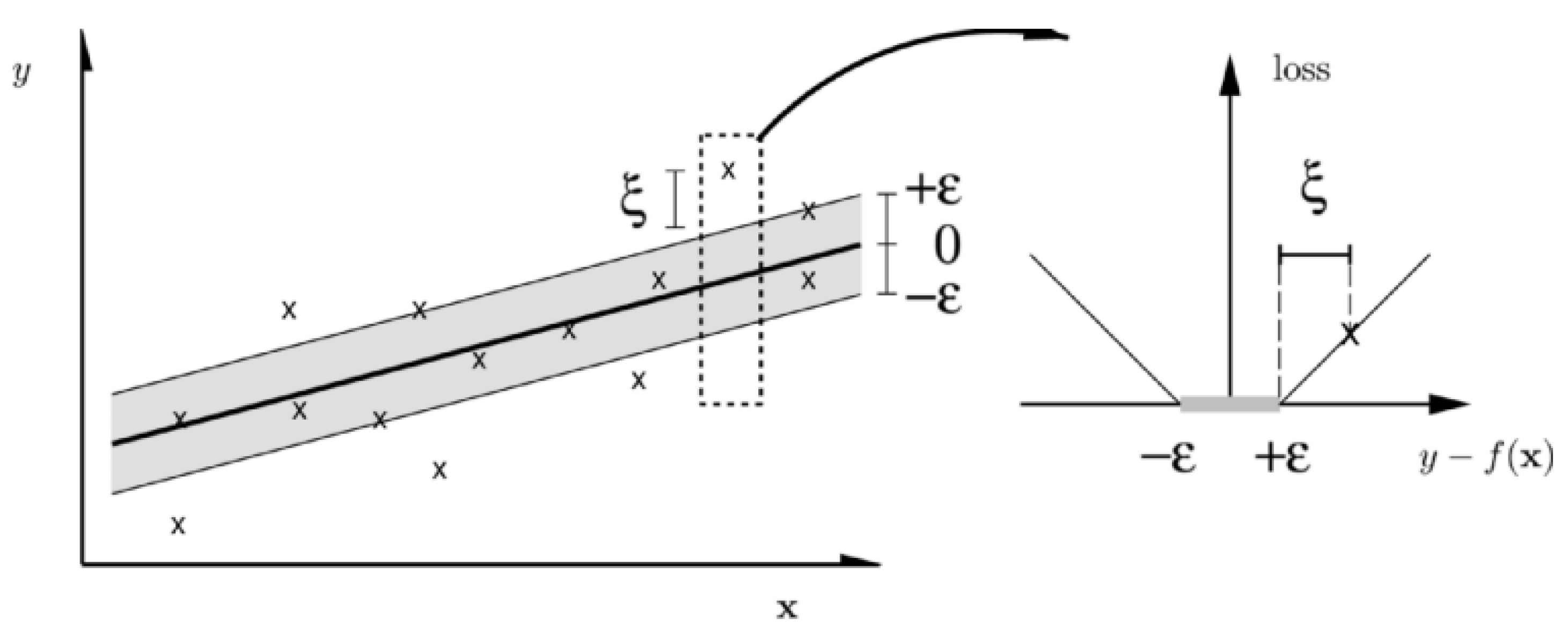
Unlike linear regression which models an outcome variable based on one predictor, MLR attempts to model the relationship between two or more independent variables and a dependent variable by mapping a linear equation into the observed data [47]. MLR models can be described using Equation (1), in which k predictors are noted as x_i1, x_i2, … x_ik, Y is the target variable, and α₀, α₁, … α_k are regression coefficients:

Y = α₀ + α₁xi₁ + α₂xi₂ + … + α_kx_ik

(1)

The model determines coefficients by minimising the sum of the square of residuals for $n$ samples of data, where every sample has k predictors and a projected target variable $y_i$, which is described in Equation (2) in which e_i is the residual error [47]:

$${\displaystyle \sum }_{i=1}^n{e}_i^2={{\displaystyle \sum }}_i^n {\left(y_i-{\alpha }_0-{\displaystyle \sum }_{j=1}^k{\alpha }_j{x}_{ij}\right)}^2$$

(2)

3.2. SVR Algorithm

SVR uses the same principles as the Support Vector Machine (SVM) to address problems in regression analysis. The basic idea behind SVR is to find the best separation line between two classes, which is known as a hyperplane. This hyperplane is mapped between two boundary lines (led by the support vectors) to form a penalty zone around the majority of the data by minimizing the prediction error (Figure 2). This zone allows a certain limit where errors outside the acceptance zone are penalized depending on their distance from the boundaries. The governing equation of the SVR algorithm is shown in the following equations [44]:

$$min \frac{1}{2}{w}^{T}w+C\left[v\mathsf{\epsilon }+\frac{1}{2}{\displaystyle \sum }_{i=1}^n\left({\xi }_i+{\xi }_i^{*}\right) \right]$$

(3)

$$\mathrm{Subject}\mathrm{to}:\left\{\begin{array}{c}{y}_i-w^T\Phi \left(x_i\right)-b\le \epsilon +{\xi }_i\\ w^T\Phi \left(x_i\right)+b-y_i-\le \epsilon +{\xi }_i^{*}\\ {\xi }_{i, }{\xi }_i^{*}\ge 0;=1, \dots \dots ,n; \epsilon \ge 0\end{array}\right.$$

(4)

where ‘C’ is the regularisation term, ‘w’ is the vector of parameters associated with the support vectors, ‘b’ is a constant, and ‘ξ’ the slack variable of errors out of ‘ɛ’ precision, which is optimized by the parameter ‘v’. The ‘i’ index labels the n cases. The term ‘ϕ(x_i)’ represents the input transformation data using a kernel K(x_i,x_j) at feature space, from which (X_i, X_j) = ϕ(x_i).ϕ(x_j) [44].

3.3. LASSO Regression Algorithm

LASSO regression works based on both feature selection and regularization techniques to escalate the prediction accuracy and interpretability of the regression model by eliminating irrelevant variables. In this method, regularization is applied to shrink some of the coefficients of the regression toward zero by forcing the residual sum of squares subject to the sum of the absolute value of the coefficients being less than a constant value t. During the feature selection process, the variables with non-zero coefficients (the most relevant ones) after the shrinkage process are considered as part of the model [45]. The regression model minimizes the following equation:

$$argmi{n}_{\beta }{\left|\right|y-{\displaystyle \sum }_{j=1}^p{x}_j{\beta }_j\left|\right|}^2+t{\displaystyle \sum }_{j=1}^p\left|{\beta }_j\right|$$

(5)

where ${\displaystyle \sum }_{j=1}^p\left|{\beta }_j\right|$ is the L1 regularization penalty on the coefficient β_j [45] and t ≥ 0 is a tuning parameter which controls the amount of shrinkage applied to the estimates. A t equal to zero results in keeping all of the variables.

3.4. XGBoost Regression Algorithm

XGBoost was first proposed in 2014 and has been continuously improved by other researchers [48,49]. This model is a learning framework based on Boosting Tress models. Each tree is formed by learning from the error of the previous trees in an attempt to improve its performance. The improvement occurs using an initial forming of the loss function of the earlier tree, which is defined as the deviation of the actual and predicted value, (Equations (6) and (7)). In the next step, it minimises the loss function using an estimation of the negative gradient as shown in Equation (8). The second is fitted to the negative gradient and predicted values, obtained from the first tree, and is updated with the addition of the predicted results obtained from the second tree [48]. This sequential process continues until the algorithm reaches a pre-defined number of trees [49] as follows:

$$L=\left(y, F\left(x\right)\right)=\frac{{\left(y-F\left(x\right)\right)}^2}{2}$$

(6)

$$J={\displaystyle \sum }_{i=1}^{n}L(y_i, F\left(x_i\right))$$

(7)

$$y_i-F\left(x_i\right)=-\frac{\partial J}{\partial F\left(x_i\right)}$$

(8)

where $y$ is the true value of the target variable, $F\left(x\right)$ is the projected value of the target variable, and $n$ is the number of samples in Equations (6)–(8).

4. Methodology

4.1. Data Collection

About 120 datasets of thermal insulation materials involving material density ($\rho )$, thermal conductivity ($\lambda )$, EE, and GWP were collected. The data were collected from past scientific literature reviews which only considered the Environmental Product Declaration (EPD) and other reputable databases such as the Okobaudat and Ecoinvent databases. Data with functional units of 1 m² with a resistance = 1 m² K/W were adopted for consistency in datasets. It was necessary to classify the dataset to the features (independent variables) and the target (dependent variable). Hill et al. [41] found a high correlation between EE and GWP, likewise, Grazieschi et al. [9] presented regression charts that showed a good relationship between thermal conductivity and density—the two constituents of the functional unit—and GWP. In this study, the $\rho$, $\lambda$, and EE of the materials were, therefore, used as the features and the GWP was used as the target. As already mentioned, since this study was not on the comparison of the environmental impact of the thermal insulation materials, but on models to predict the future environmental impact of these materials, all data on the thermal insulation materials were included. These materials range from inorganic, organic non-renewable, and organic renewable (

Table 1. Dataset of the thermal Insulation materials.

S/N	Insulation	Density (kg/m3)	Thermal Conductivity (W/mk)	Embodied Energy (MJ/kg)	GWP (KgC02eq/kg)	Ref.
1	EPS foam slab	30	0.038	105.49	7.34	[24]
2	Rockwool	60	0.040	26.39	1.51	[24]
3	Polyurethane foam	30	0.032	103.78	6.79	[24]
4	Cork slab	150	0.049	51.52	0.81	[24]
5	Cellulose fibre	50	0.040	10.49	1.83	[24]
6	Wood wool1	180	0.070	20.27	0.12	[24]
7	Stone wool1	45	0.330	63.00	3.62	[9,50]
8	Stone wool2	70	0.330	64.00	5.85	[9,42]
9	Stone wool3	35	0.400	53.09	2.77	[9,51]
10	Glass wool1	12	0.310	37.00	1.62	[9,50]
11	Glass wool2	27	0.450	90.00	8.63	[9,42]
12	Glass wool3	20	0.450	134.17	7.70	[9,51]
13	Fibre Glass	64	0.450	28.00	1.35	[9,52]
14	XPS1	34	0.031	144.00	5.52	[9,50]
15	XPS2	38	0.036	75.00	5.45	[9,42]
16	XPS3	35	0.032	127.31	13.22	[9,51]
17	XPS4	36	0.033	100.97	6.11	[9,15]
18	XPS5	36	0.035	98.11	5.21	[9,38]
19	Polyisocyanurate1	35	0.040	147.00	10.4	[9,50]
20	Polyisocyanurate2	32	0.022	81	5.83	[9,42]
21	Polyisocyanurate3	33	0.022	99.63	6.51	[9,51]
22	Polyisocyanurate4	33	0.022	63.61	2.63	[9,15]
23	Polyisocyanurate5	33	0.022	58.97	3.33	[9,38]
24	EPS1	15	0.031	147.00	4.52	[9,50]
25	EPS2	15	0.031	85.00	6.25	[9,42]
26	EPS3	15	0.031	127.31	5.05	[9,51]
27	EPS4	15	0.031	100.87	4.18	[9,15]
28	EPS5	15	0.031	74.31	3.25	[9,38]
29	Aerogel	150	0.015	372.00	18.70	[9]
30	Vermiculite	172	0.062	148.98	10.45	[9]
31	Cork	80	0.040	4.00	0.19	[9,52]
32	Flax	40	0.042	39.50	1.70	[9,52]
33	Woodwool2	60	0.038	20.00	0.98	[9,52]
34	Mineral wool	30	0.035	82.00	4.40	[52,53]
35	Rockwool	37	0.037	16.80	1.05	[36,52]
36	Paper wool	40	0.038	20.20	0.63	[53,54]
37	VIPs	180	0.020	1016	42.00	[9,53]
38	Sheep wool1	30	0.033	23.20	0.82	[9,55]
39	Sheep wool2	30	0.033	14.70	0.05	[9,56]
40	Sheep wool3	30	0.033	13.42	0.99	[9,57]
41	Straw bale	100	0.067	0.240	0.06	[9,58]
42	Perlite	166	0.055	9.350	0.493	[9,56]
43	Kenaf	40	0.038	59.37	3.170	[36]
44	Rec. PET	30	0.035	83.72	1.783	[59,60]
45	Rec. Tex. & paper	433	0.034	267.70	14.68	[61]
46	Expanded clay	245	0.095	100.00	4.43	[9]
47	Hemp	38	0.038	130.00	−0.35	[9]
48	Cotton	30	0.039	48.00	−1.20	[9,36]
49	Textile fibre	20	0.044	15.00	1.10	[9,62]
50	Glass foam	100	0.036	153.00	9.41	[9,63]
51	Min. wood fibres	420	0.100	460.00	3.53	[9]
52	UFFI1	10	0.036	75.375	3.776	[64]
53	UFFI2	10	0.036	72.535	2.882	[65,66]
54	Glasswool4	64	0.0425	318.8	16.0	[9,41]
55	Glasswool5	64	0.0395	403.9	20.3	[9,41]
56	Glasswool6	64	0.035	552.4	27.8	[9,41]
57	Glasswool7	64	0.033	658.3	33.1	[9,41]
58	Glasswool8	64	0.044	254.8	12.2	[9,41]
59	Glasswool9	64	0.037	29.8	1.5	[9,41]
60	Glasswool10	64	0.032	707.4	30.2	[9,41]
61	Glasswool11	64	0.035	438.0	19.0	[9,41]
62	Glasswool12	64	0.04	253.7	11.4	[9,41]
63	Glasswool13	64	0.035	521.5	28.5	[9,41]
64	Glasswool14	64	0.0365	30.1	1.8	[9,41]
65	Mineralwool2	30	0.35	474.1	15.7	[9,41]
66	Mineralwool3	30	0.03676	49.0	1.2	[9,41]
67	Mineralwool4	30	0.035	81.5	4.4	[9,41]
68	Mineralwool5	30	0.039	668.7	53.7	[9,41]
69	Mineralwool6	30	0.04	1746.0	95.8	[9,41]
70	Mineralwool7	30	0.035	937.8	76.7	[9,41]
71	Mineralwool8	30	0.0375	26.4	1.6	[9,41]
72	Mineralwool9	30	0.037	13.5	1.3	[9,41]
73	Mineralwool10	30	0.04	609.7	34.4	[9,41]
74	Mineralwool11	30	0.04	1213.0	82.6	[9,41]
75	Mineralwool12	30	0.04	1941.4	141.0	[9,41]
76	Mineralwool13	30	0.037	20.8	1.5	[9,41]
77	Mineralwool14	30	0.036	465.5	25.4	[9,41]
78	Mineralwool15	30	0.0335	762.6	42.6	[9,41]
79	Mineralwool16	30	0.0335	758.4	41.4	[9,41]
80	Mineralwool17	30	0.04	465.5	25.4	[9,41]
81	Mineralwool18	15	0.04	578.9	28.8	[9,41]
82	EPS6	15	0.035	1329.6	46.34	[9,41]
83	EPS7	15	0.034	33.5	2.0	[9,41]
84	EPS8	15	0.035	1329.6	46.3	[9,41]
85	EPS9	15	0.035	1327.9	46.3	[9,41]
86	EPS10	15	0.036	26.0	2.3	[9,41]
87	EPS11	15	0.031	30.0	2.0	[9,41]
88	EPS12	15	0.035	2291.9	79.0	[9,41]
89	EPS13	15	0.035	1383.8	48.0	[9,41]
90	EPS14	24	0.035	1847.5	62.0	[9,41]
91	XPS6	24	0.031	151.1	10.2	[9,41]
92	XPS7	24	0.035	158.6	9.4	[9,41]
93	XPS8	24	0.035	161.2	9.5	[9,41]
94	XPS9	35	0.035	159.4	9.4	[9,41]
95	PUR1	31.5	0.023	241.4	15.0	[9,41]
96	PUR2	31.5	0.023	216.6	12.9	[9,41]
97	PUR3	31.5	0.026	209.4	13.1	[9,41]
98	PUR4	31.5	0.023	202.6	12.0	[9,41]
99	PUR5	31.5	0.026	204.9	12.9	[9,41]
100	PUR6	31.5	0.026	267.4	16.6	[9,41]
101	PUR7	31.5	0.026	401.2	24.9	[9,41]
102	PUR8	31.5	0.023	512.2	37.5	[9,41]
103	PUR9	-	0.023	173.5	12.2	[9,41]
104	PFFoam1	-	0.021	173.7	9.9	[9,41]
105	PFFoam2	100	0.021	178.9	10.2	[9,41]
106	Foamglass1	100	0.103	937.0	19.2	[9,41]
107	Foamglass2	100	0.082	738.9	15.2	[9,41]
108	Foamglass3	100	-	7.0	0.2	[9,41]
109	Foamglass4	30	0.041	28.8	1.3	[9,41]
110	Cellulose1	30	0.039	89.7	3.7	[9,41]
111	Cellulose2	80	0.039	100.0	2.8	[9,41]
112	Cellulose3	80	-	9768.0	1189.0	[9,41]
113	Cellulose4	80	0.039	5.3	0.2	[9,41]
114	Cellulose5	80	-	2.1	0.1	[9,41]
115	Cellulose6	80	-	6148.0	295.0	[9,41]
116	Cellulose7	80	0.049	8263.5	214.1	[9,41]
117	Cellulose8	80	0.040	4006.9	102.6	[9,41]
118	Cellulose9	80	0.042	4037.2	100.6	[9,41]
119	Cellulose10	80	0.050	7589.4	182.5	[9,41]
120	Cellulose11	80	0.038	2560.0	59.9	[9,41]
121	Cellulose12	80	0.047	4337.0	105.4	[9,41]
122	Cellulose13	80	0.044	4936.2	82.1	[9,41]

).

4.2. Data Processing

Before building the ML models, it was necessary to perform data cleaning and processing. Python 3 (ipykernel) and Scikit-learn library were used for the data processing and implementation of the ML methods. For the data processing, correlation feature selection was performed (Figure 3) to identify more relevant features to predict the target outcome. Figure 3 shows a heat map chart for the correlation of the features, with DE as the density, TC as the thermal conductivity, EE as the embodied energy, and GW as the GWP. In Figure 3, each square shows a correlation within the range of −1 to +1. The closer to −1 or +1 a box appears, and the darker, the more correlation it has with an adjacent feature. Each box has a perfect correlation to itself (the diagonal yellow boxes show that they have a perfect correlation to themselves). It can be clearly seen that EE shows the strongest correlation to GW, followed by TC, and DE shows a weak correlation. To confirm this, a quick test was run, and it was observed that DE led to poor outcomes across all the models. This is partly due to its weak correlation with GW. It was necessary to complete a second quick test after the DE was excluded from the dataset, at which time, reasonable outcomes from the algorithms were found. Therefore, in this study, the DE was excluded and only the TC and EE were considered as the independent variables and GW as the target.

In compliance with standard machine learning processes, the dataset was split into training and testing sets. The training data were used for the training of the models and the testing data were unseen by the model during the training time. Except for the MLR with uncomplicated parameter settings, hyper-parameter tuning was completed for the SVR, LASSO, and XGBoost. After hyper-parameter tuning of the SVR, the linear kernel outperformed the Radial Basis Function kernel (RBF) and the Polynomial Kernel for prediction after an initial check on this particular dataset. Likewise, hyper-parameter tuning was conducted for the LASSO regression and the ‘L’₁ values were tuned, which are the regularisation factors for an optimum hyper-parameter. The XGBoost was set to perform the automatic in-built hyper-parameter tuning as well.

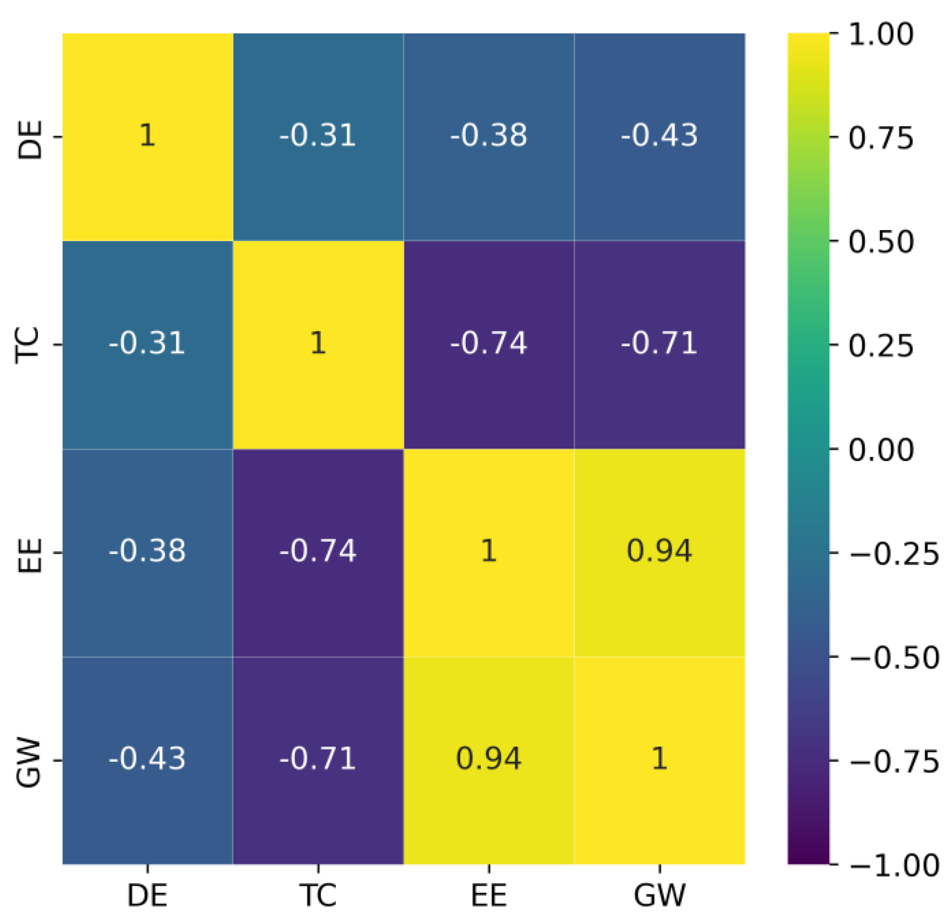
4.3. Evaluation of the Algorithms

Several metrics are used for the evaluation of machine learning algorithms. From the Scikit-learn library in Python, common metrics which provide quick comparison of models were imported including the Coefficient of Determination (R²), Root Mean Squared Error (RMSE), and Mean Absolute Error (MAE) [49,67]. The R² (Equation (9)) was used to compare the proportion of the variances in the sample variables and the predicted variables of the ML models to determine their performances. The RMSE (Equation (10)) was used to check and compare the concentration and spread of data around the regression line for each of the models, and the MAE (Equation (11)) was used for comparing the average model-performance error. MAE is claimed to be a better metric for the basis of comparison than the RMSE [68].

$$R^2=1-\frac{{{\displaystyle \sum }}_{i=1}^n{(y_i-\widehat{y_i})}^2}{{{\displaystyle \sum }}_{i=1}^n{(y_i-\overline{y})}^2}$$

(9)

$$RMSE=\sqrt{ \frac{1}{n} {\displaystyle \sum }_i^n{(y_i-\widehat{y_i})}^2}$$

(10)

$$MAE=\frac{1}{n}{\displaystyle \sum }_{i=1}^n\left|y_i-\widehat{y_i}\right|$$

(11)

In Equations (9)–(11), y is the observation value; $\overline{y}$ is the mean of observation values; $\widehat{y}$ is the predicted value; and i is the ith observation.

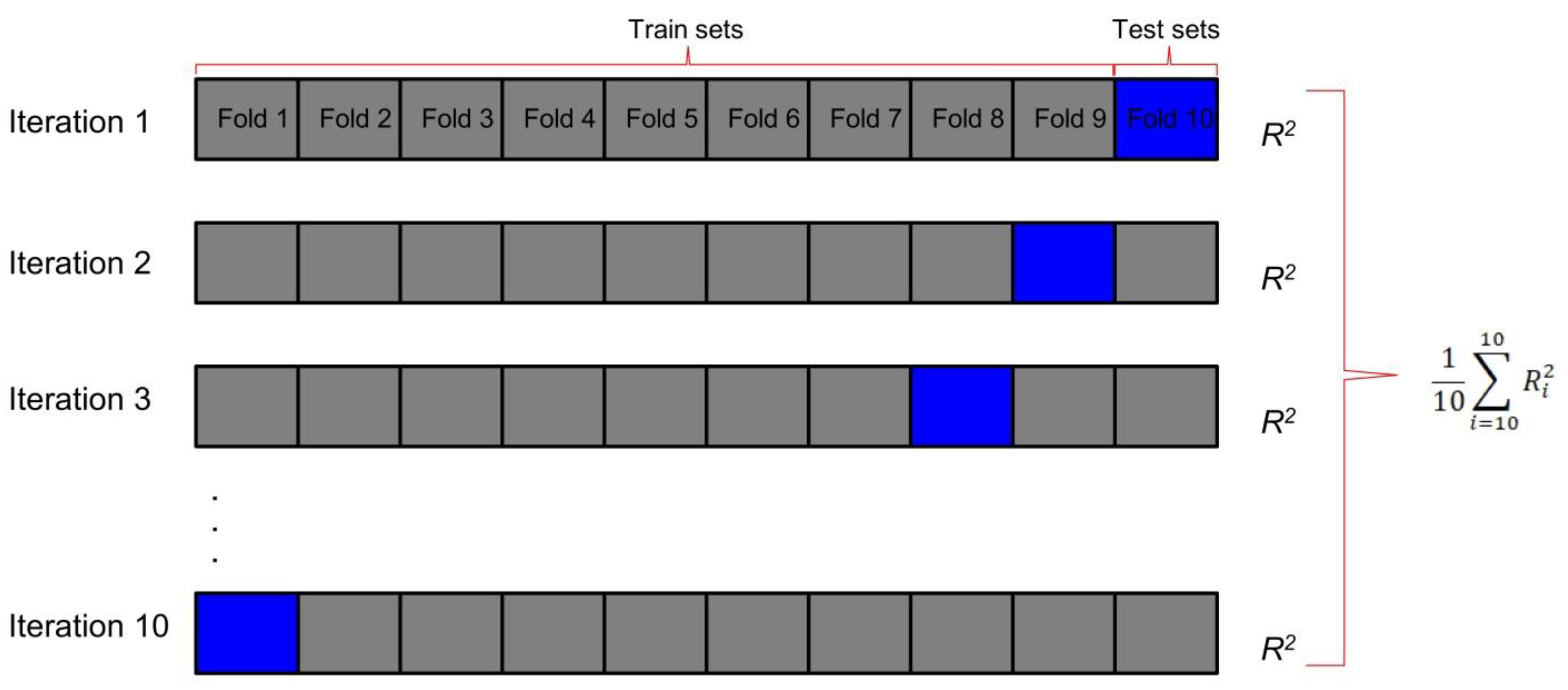
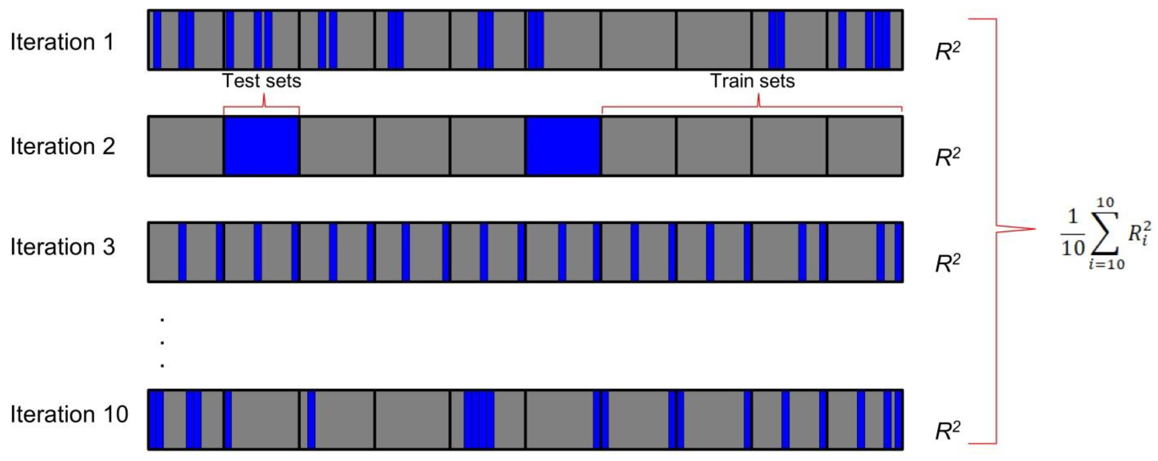
4.4. Cross-Validation

In order to prevent the models from over-fitting, cross-validations were conducted to validate the estimated evaluation metrics. In this study, we only pay particular attention to R² values in the cross-validation procedures. In compliance with standard machine learning procedures, as mentioned earlier, we had initially performed a validation process known as the ‘Holdout’ validation, where the data were split into training data (80%) and testing/validation data (20%). Although, this process may not be robust enough as some of the training data get leaked into the testing data as a result of passing just one iteration; hence, a possibility of model over-fitting may occur. Therefore, two more robust cross-validations were performed including the K-Fold and Monte-Carlo (Shuffle split) cross-validation techniques. The K-Fold cross-validation works using a technique where the whole dataset can be initially split into K parts of equal sizes, and each split is known as a fold, and K can be any integer. K-1 folds are used for training the model. The models were set for 10 iterations where every fold was used for validation and the others were left out for training (K-1) until the technique exhausted all the iterations and each fold was used once (Figure 4). The Monte-Carlo cross-validation is an extension of the traditional Holdout validation, where the data are split into the conventional training and testing sets.

In this study, the data were split into 80% training and 20% testing sets. Again, the models were set for 10 iterations, and the technique automatically performed random shuffling across the iterations (Figure 5). In addition to that, the models were fitted to the training data in each of the iterations, and the accuracy of the fitted models was calculated using the testing data. The mean value of all the test scores (R² scores) was finally recorded to determine the performance of each model.

5. Results and Discussion

This section presents the various results of the prediction outcomes of the GWP, the evaluation metrics, and prediction errors, and also the cross-validations. First of all, the observed and predicted results of the GWP of the models were compared with respect to the Holdout validation of the test samples. It can be observed that the observations and the predicted curves in all the models have similar trends. For this validation test, the MLR and LASSO regressions showed R² scores of 0.83, while the SVR presented an R² of 0.82, and the XGBoost showed an R² of 0.91, as seen in Figure 6a–d. Generally, all the models performed well for the dataset in this initial R² evaluation.

Moreover, considering the plots showing the testing data of the GWP on the y-axes and their place values (the randomised 20% of the whole dataset) on the x-axes, it can be observed that values 10–15, 17, 22, and 24 on the x-axes were approximately predicted better than the other values. These values coincide with the values of the GWP on the y-axes and are thus: PUR₄, PUR₃, PUR₂, Polyurathane foam, XPS_6, Cellulose_7, PFFoam_2, XPS₅ and Cellulose₈, respectively. A demonstration of these correlations can be clearly seen in

Table 2. Randomised Testing Data for the Holdout Validation.

Insulations	Testing Data Place Values	GWP (KgC02eq/kg)
PUR1	1	15.0
Glasswool5	2	20.3
Glasswool10	3	30.2
Cellulose11	4	59.9
Mineralwool12	5	141.0
Hemp	6	−0.35
Flax	7	1.7
Mineralwool18	8	28.8
Textile fibre	9	1.1
PUR4	10	12.0
PUR3	11	13.1
PUR2	12	12.9
Polyurethane foam	13	6.79
XPS6	14	10.2
Cellulose7	15	214.1
Glasswool7	16	33.1
PFFoam2	17	10.2
PUR8	18	37.5
Mineralwool5	19	53.7
Glasswool13	20	28.5
Mineralwool16	21	41.4
XPS5	22	5.21
EPS7/EPS11	23	2.0
Cellulose8	24	102.6

. This means that for these models to perform optimally in the regressions, they needed more training using data similar to the randomised testing data, which gave better regressions.

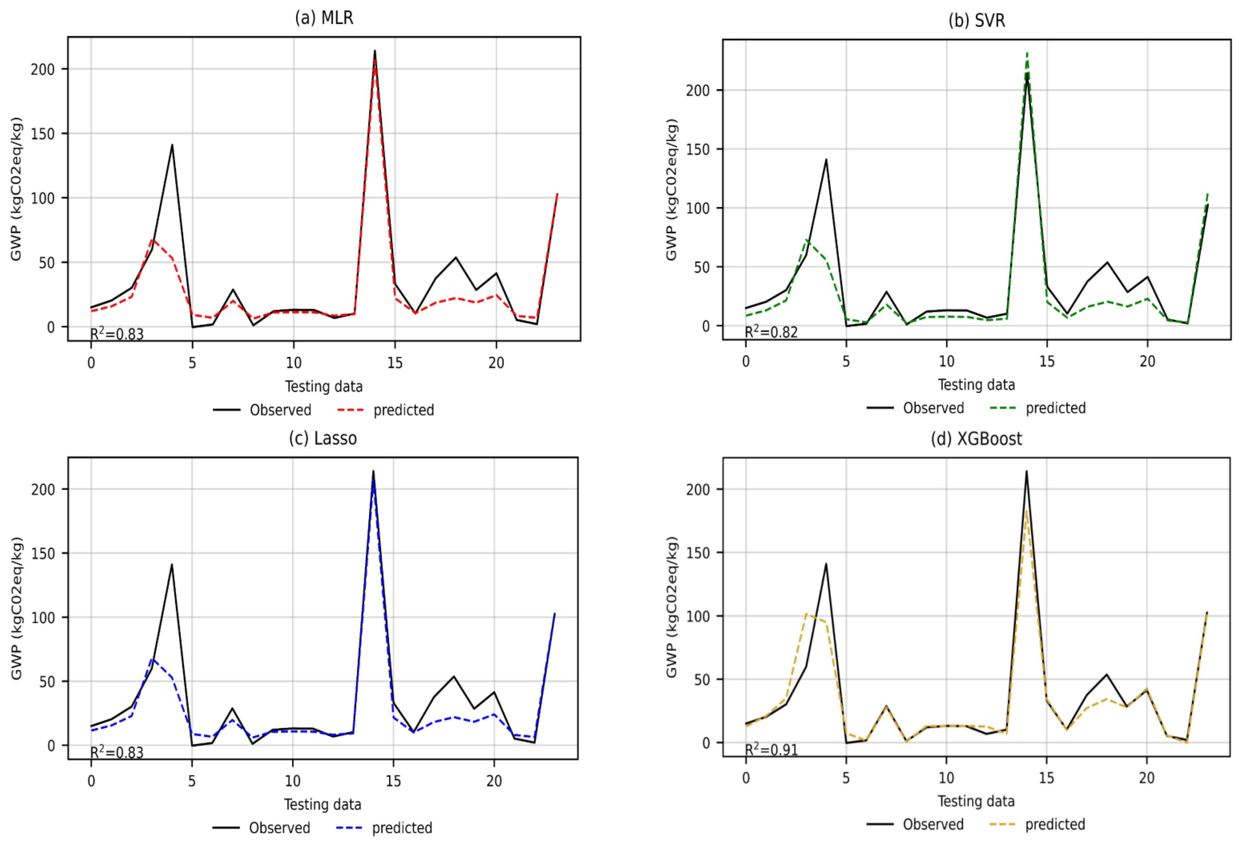
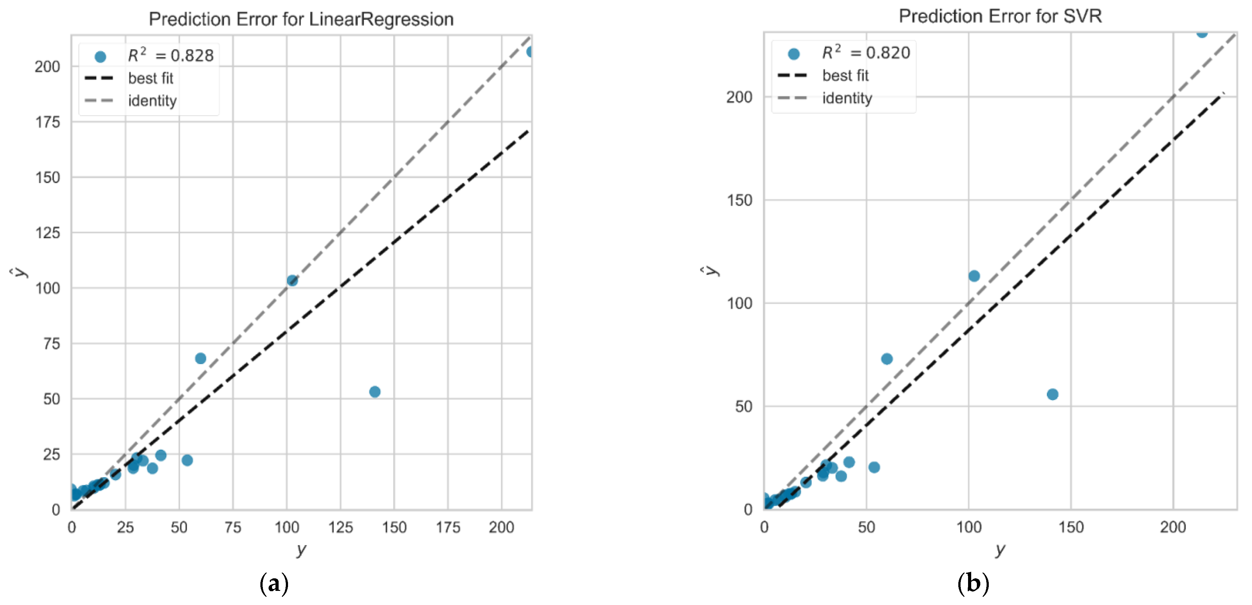
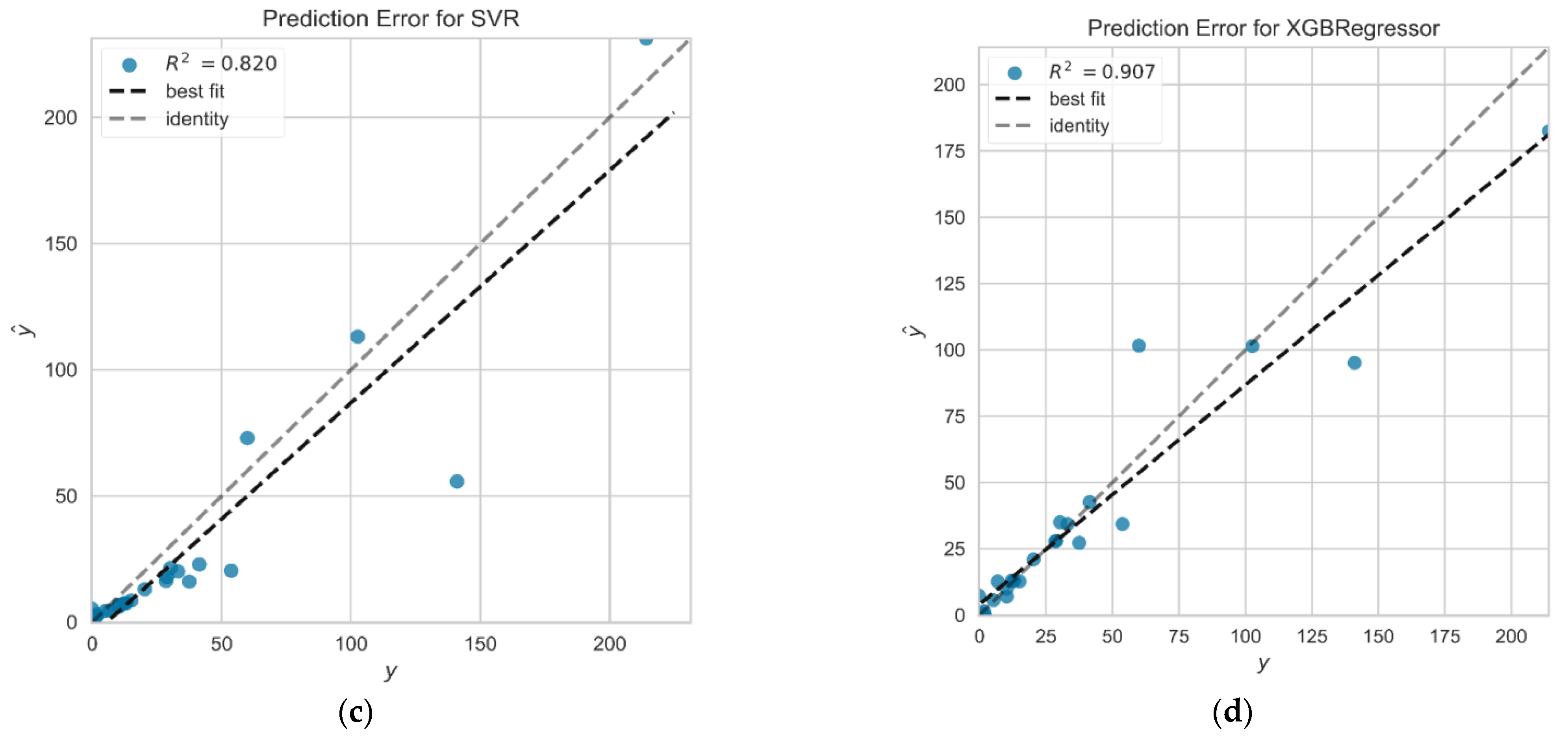
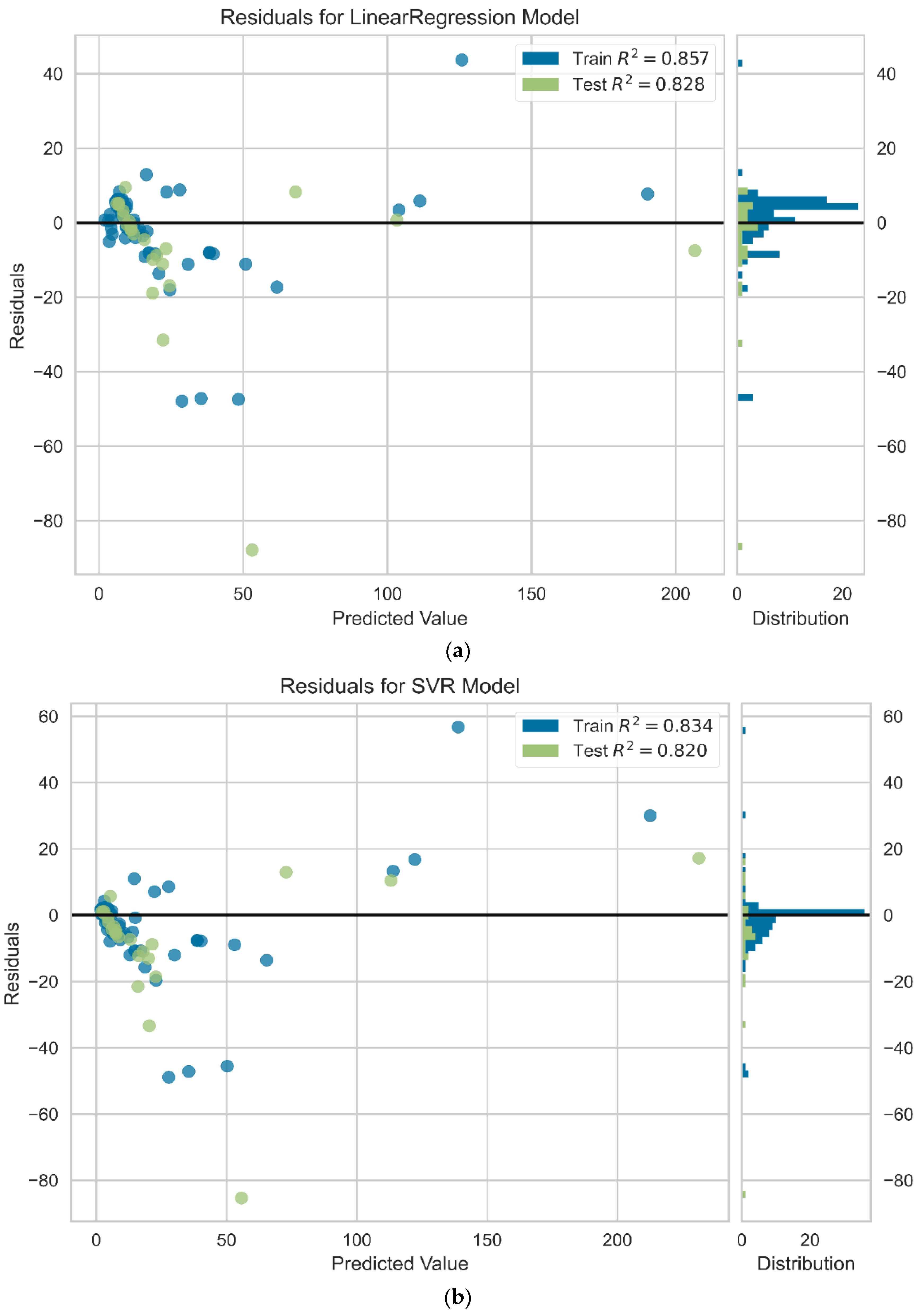
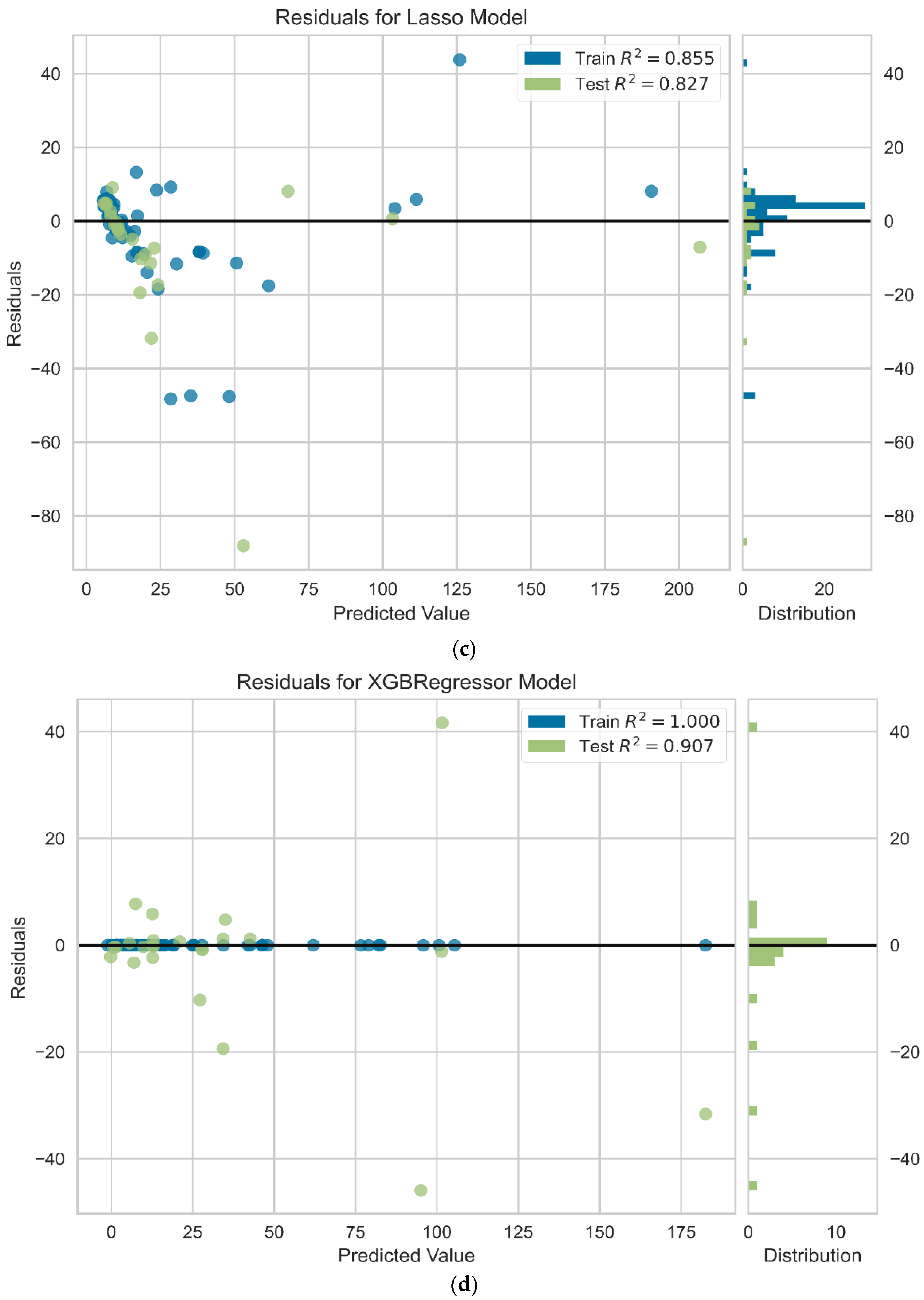
5.1. Prediction Errors

After the initial evaluations of the regression models, tests were conducted to show the extent of the variances and biases between the actual GWP (y) and the predicted GWP ($\widehat{y}$) of the dataset used in all of the models (Figure 7a–d). It can be observed that there is a trade-off between the biases and the variances in the MLR, LASSO, and SVR models compared to the XGBoost model, which has high variance and means that the XGBoost model is prone to overfitting. The MLR, LASSO, and SVR models have similar trends in their errors. After removing the few outliers from the first three models that explained the high values of the MAE (Table 2), there was more confidence in how the three models fit the data points. An arbitrary line (identity) was drawn, which was set to be automatically generated, and in comparison to the regression lines (best fit), one can visually observe where the models produced larger errors in the prediction process.

5.2. Residuals of Training and Testing Sets

The concentration and distribution of the residuals were checked along the regression lines for the training and testing datasets, and it can be observed that a large portion of the residuals was randomly distributed around the zero axis, confirming the homoscedasticity of the models, i.e., similar variances in the training and testing datasets (Figure 8a–c). However, even with the homoscedastic nature, higher values of RMSE were found (Table 2). This was likely due to some possible outliers having huge margins away from the regression lines in the dataset, i.e., with larger errors. It was further confirmed that the RMSE and MAE were highly vulnerable to these outliers after a quick test was conducted by screening out some observations considered to be outliers as far as possible. After this quick test, the RMSE significantly reduced from >20 to <2.2, and the MAE significantly reduced from about >6.7 to <1.7 for the testing/validation set. Although, it was impossible to identify all the outliers due to the nature of the dataset. Generally, the MLR, SVR, and LASSO regression models predict optimally, i.e., neither overfitting nor underfitting. Evidence of this was the slight difference in R² scores, which were unaffected by the outliers, between the training and testing sets. Conversely, at this point in this Section, it is essential to re-emphasise that the XGBoost model obviously overfitted the dataset in the training stage (Figure 8d). Evidence of this was the high variances (R² score of 1.0) and complete non-errors in the training stage, with corresponding large errors in the testing/validation stage (high values of RMSE and MAE), as shown in

Table 3. Evaluation Metric Scores of the Models.

Metrics		MLR	SVR	LASSO	XGBOOST
	R2	0.86	0.83	0.86	1.00
		0.83	0.82	0.83	0.91
Train set Test set	RMSE	11.22	12.12	11.31	0.00
		20.44	20.93	20.54	15.06
	MAE	6.69	6.16	6.68	0.01
		10.75	12.20	10.56	7.64

.

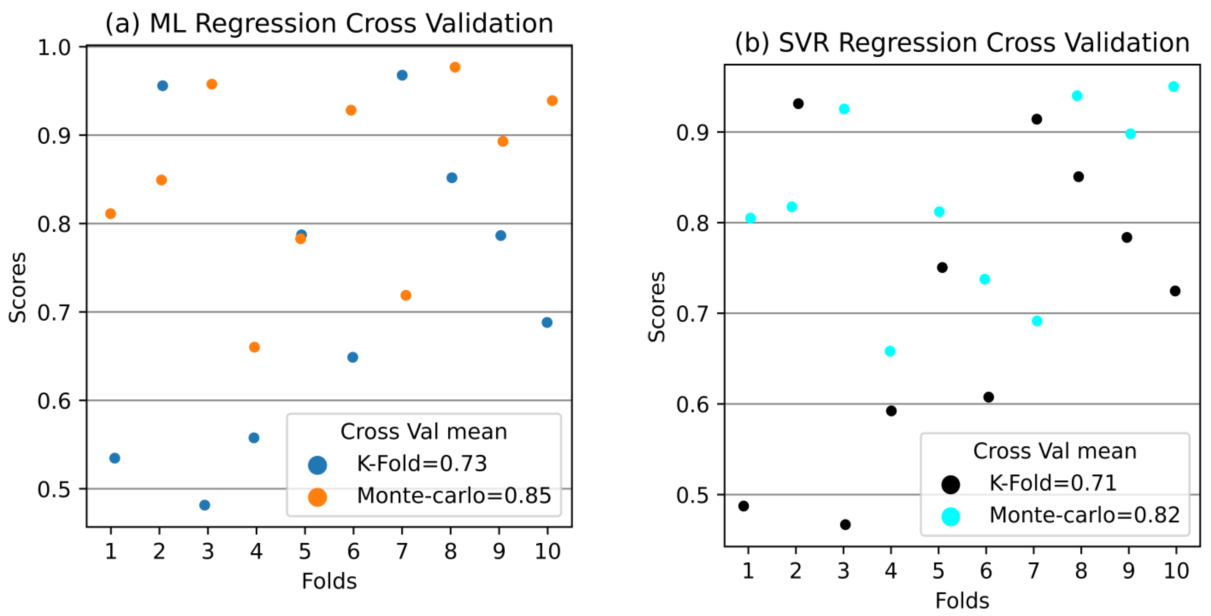
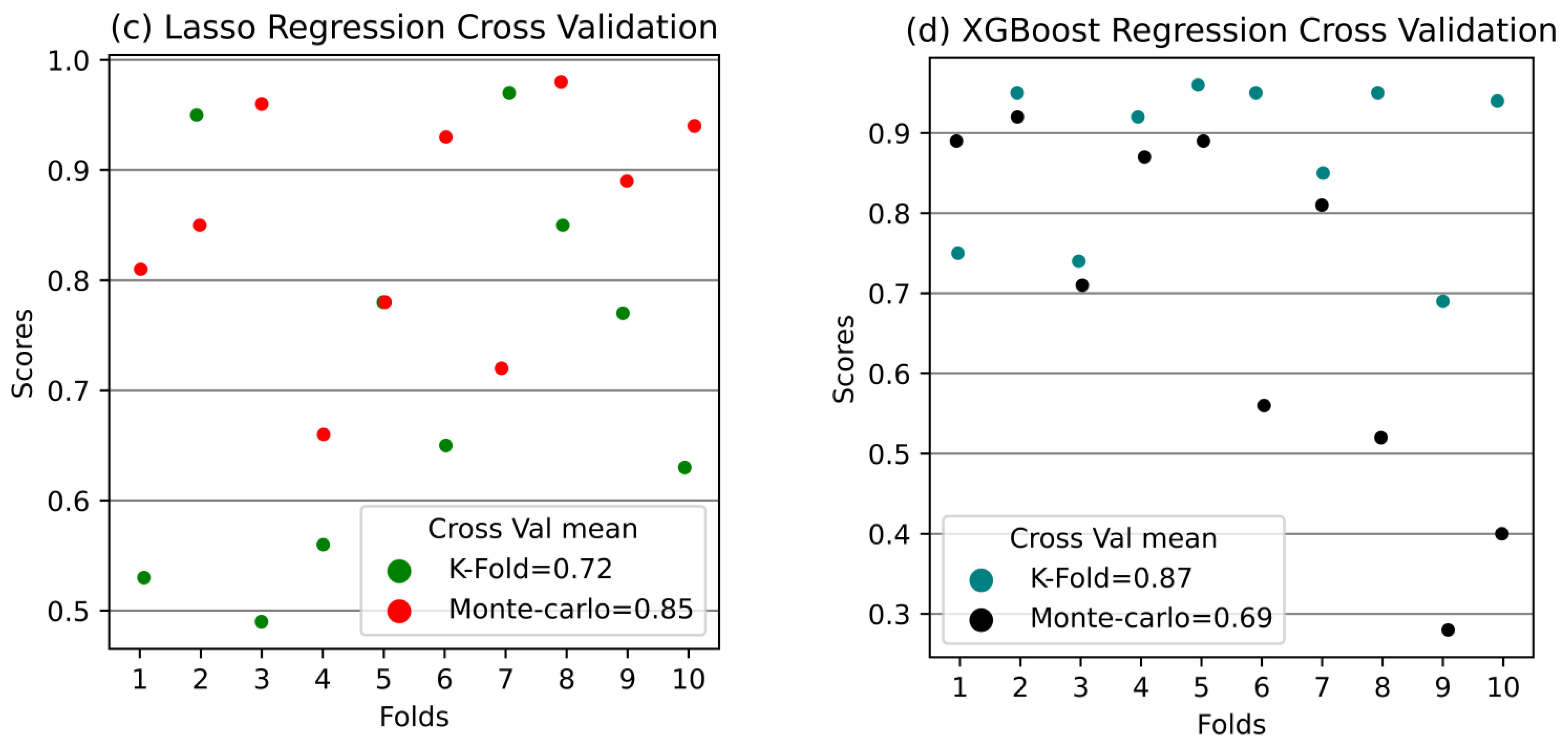
5.3. K-Fold and Monte-Carlo Cross-Validations

It was necessary to run final validations (the cross-validations) on the whole dataset in addition to the Holdout validation as earlier mentioned in order to reliably ensure that the models were not overfitted on both the training and testing datasets. Figure 9a–d shows the comparison of the K-fold and Monte-Carlo cross-validations across all the models. It can be seen that there is a similar match in the performance of the Monte-Carlo mean R² scores of the MLR (0.85), SVR (0.82), and LASSO (0.85) in comparison to the Holdout validation. Although, the K-Fold cross-validations show slight differences in the models compared to the Monte-Carlo and the Holdout (MLR = 0.73, SVR = 0.71, and LASSO = 0.72) results. Based on the R² scores from the cross-validations, it can be concluded that the three models performed well. On the other hand, it can be seen that the XGBoost model depicts an opposite trend, where the Monte-Carlo cross-validation shows an R² mean score of 0.69 and the K-Fold cross-validation shows a score of 0.86. This means that there is a discrepancy in the cross-validations and the Holdout validation for the XGBoost model.

In addition,

Table 4. Generated 10 folds validation values for K-Fold and Monte-Carlo in Python.

Models	R2 Scores
MLR	K-Fold
	0.53463136, 0.95586595, 0.4815178, 0.5576389, 0.7872245,
	0.64872736, 0.96775078, 0.85180267, 0.78641759, 0.68811461
	Monte-Carlo
	0.81117444, 0.84924004, 0.95764438, 0.66015406, 0.78274875,
	0.92822053, 0.71882231, 0.97685173, 0.89295711, 0.93901005
SVR	K-Fold
	0.48734585, 0.93125042, 0.46685477, 0.5923367, 0.75049093, 0.60751874, 0.91412253, 0.85066154, 0.78367544, 0.7246273
	Monte-Carlo
	0.80502996, 0.81745197, 0.92541027, 0.65821522, 0.81205356, 0.73761791, 0.69151795, 0.9399861, 0.89805164, 0.95013416
LASSO	K-Fold
	0.53224332, 0.95444857, 0.48598915, 0.56007886, 0.7832618, 0.64958839, 0.96626447, 0.85139013, 0.76666582, 0.63332968
	Monte-Carlo
	0.80966647, 0.84666507, 0.95558787, 0.658763, 0.78283893, 0.92704338, 0.71542824, 0.97566539, 0.89436693, 0.94277419
XGBoost	K-Fold
	0.7543402, 0.95840054, 0.73656183, 0.92822975, 0.95850548, 0.94758277, 0.85313272, 0.94945763, 0.68740307, 0.94040784
	Monte-Carlo
	0.88943108, 0.91617215, 0.70638463, 0.87221572, 0.89104877, 0.56351587, 0.81172492, 0.52429175, 0.27620335, 0.40165315

shows the in-depth analysis of the R² scores of the cross-validations, and one can observe that in each of the 10 folds, the Monte-Carlo values are higher than the K-Fold values for all the models, except for the XGBoost model. This is interesting to note because the Monte-Carlo cross-validation is more desirable over most cross-validation techniques, owing to its capacity to evaluate different models according to their predictive capability using many different combinations of validation datasets [69]. This is an advantage in this task as it lends credence to the overall performance of the models’ reliability when the Monte-Carlo scores are found to be higher.

6. Conclusions

In this study, in an attempt to contribute to mitigating the current global energy crisis, machine learning regression models were developed to predict the GWP of insulation materials. This will provide the basic guidelines for manufacturers and energy policymakers, thus allowing them to understand the potential environmental impacts of future insulation materials that could be supplied to the market. Below are the key findings of this paper:

• The GWP of thermal insulation materials is hugely dependent on the EE, and it can vary widely for different types of insulation. This, in turn, causes variations in the nature of the dataset. Large datasets that compensate for all these variations will surely allow regression models to generalise properly while reducing some possible prediction errors, such as in the RMSE and the MAE, caused by outliers that have large margins with respect to a regression line.
• In terms of the size of datasets used in this study, we found that MLR, SVR, and LASSO regression methods provide satisfactory prediction capabilities for unseen datasets. However, there is less confidence in the XGBoost regression method due to the overfitting of the training data.
• It would be more encouraging to gather large data of this kind for better accuracy in future studies. This will be possible when more manufacturers provide access to environmentally related information on thermal insulation materials.

References

1. Asdrubali, F.; D’Alessandro, F.; Schiavoni, S. A review of unconventional sustainable building insulation materials. Sustain. Mater. Technol. 2015, 4, 1–17. [Google Scholar] [CrossRef]
2. United Nation Environment Programme. Environment for Development. Available online: http://www.unep.org/sbci/AboutSBCI/Background.asp (accessed on 7 September 2022).
3. U.S. Department of Energy. Building Energy Data Book. Available online: http://buildingsdatabook.eren.doe.gov/ChapterIntro1.aspx (accessed on 7 September 2022).
4. European Commission. Available online: http://ec.europa.eu/energy/en/topics/energy-efficiency/buildings (accessed on 7 September 2022).
5. Lechtenböhmer, S.; Schüring, A. The potential for large scale savings from insulating residential buildings in the EU. Energy Effic. 2009, 4, 257–270. [Google Scholar] [CrossRef]
6. Nyers, J.; Kajtar, L.; Tomić, S.; Nyers, A. Investment-savings method for energy economic optimization of external wall thermal insulation thickness. Energy Build. 2015, 86, 268–274. [Google Scholar] [CrossRef]
7. Alam, M.; Singh, H.; Limbachiya, M.C. Vacuum Insulation Panels (VIPs) for building construction industry—A review of the contemporary developments and future directions. Appl. Energy 2011, 8, 592–3602. [Google Scholar] [CrossRef] [Green Version]
8. Ahmad, E.H. Cost analysis and thickness optimization of thermal insulation materials used in residential buildings in Saudi Arabia. In Proceedings of the 6th Saudi Engineering Conference, Dhahran, Saudi Arabia, 14–17 December 2002. [Google Scholar]
9. Grazieschi, G.; Asdrubali, F.; Thomas, G. Embodied energy and carbon of building insulating materials: A critical review. J. Clean. Prod. 2021, 2, 100032. [Google Scholar] [CrossRef]
10. Dodoo, A.; Gustavsson, L.; Sathre, R. Life cycle primary energy implication of retrofitting a wood-framed apartment building to passive house standard. Resour. Conserv. Recycl. 2010, 54, 1152–1160. [Google Scholar] [CrossRef]
11. Blengini, G.A.; Di Carlo, T. Energy-saving policies and low-energy residential buildings: An LCA case study to support decision makers in piedmont (Italy). Int. J. Life Cycle Assess. 2010, 15, 652–665. [Google Scholar] [CrossRef]
12. Chastas, P.; Theodosiou, T.; Bikas, D. Embodied energy in residential buildingstowards the nearly zero energy building: A literature review. Build. Environ. 2016, 105, 267–282. [Google Scholar] [CrossRef]
13. Thormark, C. A low energy building in a life cycle—Its embodied energy, energy need for operation and recycling potential. Build. Environ. 2002, 37, 429–435. [Google Scholar] [CrossRef]
14. Asdrubali, F.; Baggio, P.; Prada, A.; Grazieschi, G.; Guattari, C. Dynamic life cycle assessment modelling of a NZEB building. Energy 2020, 191, 116489. [Google Scholar] [CrossRef]
15. Biswas, K.; Shrestha, S.S.; Bhandari, M.S.; Desjarlais, A.O. Insulation materials for commercial buildings in North America: An assessment of lifetime energy and environmental impacts. Energy Build. 2016, 112, 256–269. [Google Scholar] [CrossRef] [Green Version]
16. Sargam, Y.; Wang, K.; Cho, I.H. Machine learning based prediction model for thermal conductivity of concrete. J. Build. Eng. 2021, 34, 101956. [Google Scholar] [CrossRef]
17. Valipour, B.G.; Bahramian, A.R. Applying machine learning for predicting thermal conductivity coefficient of polymeric aerogels. J. Therm. Anal. Calorim. 2021, 147, 6227–6238. [Google Scholar]
18. Ciambrone, D.F. Environmental Life Cycle Assessment; CRC Press Inc.: Boca Raton, FL, USA, 1997. [Google Scholar]
19. Joshi, S. Environmental life-cycle assessment using input–output techniques. J. Ind. Ecol. 1999, 32, 95–120. [Google Scholar] [CrossRef]
20. Hauschild, M.Z.; Rosenbaum, R.K.; Olsen, S.I. Life Cycle Assessment; Springer International Publishing: Cham, Switzerland, 2018. [Google Scholar]
21. Buyle, M.; Braet, J.; Audenaert, A. Life cycle assessment in the construction sector: A review. Renew. Sustain. Energy Rev. 2013, 26, 379–388. [Google Scholar] [CrossRef]
22. Mattoni, B.; Bisegna, F.; Evangelisti, L.; Guattari, C.; Asdrubali, F. Influence of LCA procedure on the green building rating tools outcomes. IOP Conf. Ser. Mater. Sci. Eng. 2019, 609, 072044. [Google Scholar] [CrossRef]
23. Zhao, C.Z.; Liu, Y.; Ren, S.W.; Zhang, Y.J. Life aycle assessment of typical Glass Wool production in China. Mater. Sci. Forum 2018, 913, 998–1003. [Google Scholar] [CrossRef]
24. Bribián, I.Z.; Capilla, A.V.; Usón, A.A. Life cycle assessment of building materials: Comparative analysis of energy and environmental impacts and evaluation of the eco-efficiency improvement potential. Build. Envron. 2011, 46, 1133–1140. [Google Scholar] [CrossRef]
25. Antoniadou, P.; Giama, E.; Boemi, S.-N.; Karlessi, T.; Santamouris, M.; Papadopoulos, A. Integrated evaluation of the performance of composite cool thermal insulation materials. Energy Procedia 2015, 78, 1581–1586. [Google Scholar] [CrossRef] [Green Version]
26. Cozzarini, L.; Marsich, L.; Ferluga, A.; Schmid, C. Life cycle analysis of a novel thermal insulator obtained from recycled glass waste. Dev. Built Environ. 2020, 3, 100014. [Google Scholar] [CrossRef]
27. Gomes, R.; Silvestre, J.D.; de Brito, J. Environmental life cycle assessment of the manufacture of EPS granulates, lightweight concrete with EPS and high-density EPS boards. J. Build. Eng. 2020, 28, 10103. [Google Scholar] [CrossRef]
28. Dickson, T.; Pavía, S. Energy performance, environmental impact and cost of a range of insulation materials. Renew. Sustain. Energy Rev. 2021, 140, 110752. [Google Scholar] [CrossRef]
29. Rocchi, L.; Paolotti, L.; Fagioli, F.F.; Boggia, A. Production of insulating panel from pruning remains: An economic and environmental analysis. Energy Procedia 2018, 147, 145–153. [Google Scholar] [CrossRef]
30. Nakano, K.; Ando, K.; Takigawa, M.; Hattori, N. Life cycle assessment of woodbased boards produced in Japan and impact of formaldehyde emissions during the use stage. Int. J. Life Cycle Assess. 2018, 23, 957–969. [Google Scholar] [CrossRef]
31. Sierra-Pérez, J.; Boschmonart-Rives, J.; Dias, A.C.; Gabarrell, X. Environmental implications of the use of agglomerated cork as thermal insulation in buildings. J. Clean. Prod. 2016, 126, 97–107. [Google Scholar] [CrossRef]
32. Demertzi, M.; Sierra-Pérez, J.; Paulo, J.A.; Arroja, L.; Dias, A.C. Environmental performance of expanded cork slab and granules through life cycle assessment. J. Clean. Prod. 2017, 145, 294–302. [Google Scholar] [CrossRef]
33. Arrigoni, A.; Pelosato, R.; Melià, P.; Ruggieri, G.; Sabbadini, S.; Dotelli, G. Life cycle assessment of natural building materials: The role of carbonation, mixture components and transport in the environmental impacts of hempcrete blocks. J. Clean. Prod. 2017, 149, 1051–1061. [Google Scholar] [CrossRef]
34. Sinka, M.; Van den Heede, P.; De Belie, N.; Bajare, D.; Sahmenko, G.; Korjakins, A. Comparative life cycle assessment of magnesium binders as an alternative for hemp concrete. Resour. Conserv. Recycl. 2018, 133, 288–299. [Google Scholar] [CrossRef]
35. Zampori, L.; Dotelli, G.; Vernelli, V. Life cycle assessment of hemp cultivation and use of hemp-based thermal insulator materials in buildings. Environ. Sci. Technol. 2013, 47, 7413–7420. [Google Scholar] [CrossRef]
36. Ardente, F.; Beccali, M.; Cellura, M.; Mistretta, M. Building energy performance: A LCA case study of kenaf-fibres insulation board. Energy Build. 2008, 40, 1–10. [Google Scholar] [CrossRef]
37. Struhala, K.; Stránská, Z.; Sedlák, J. LCA of Fibre Flax Thermal Insulation. Appl. Mech. Mater. 2016, 824, 761–769. [Google Scholar] [CrossRef]
38. Pargana, N.; Pinheiro, M.D.; Silvestre, J.D.; de Brito, J. Comparative environmental life cycle assessment of thermal insulation materials of buildings. Energy Build. 2014, 82, 466–481. [Google Scholar] [CrossRef]
39. Resalati, S.; Okoroafor, T.; Henshall, P.; Simões, N.; Gonçalves, M.; Alam, M. Comparative life cycle assessment of different vacuum insulation panel core materials using a cradle to gate approach. Build. Environ. 2021, 188, 107501. [Google Scholar] [CrossRef]
40. Pinto, I.; Silvestre, J.D.; de Brito, J.; Júlio, M.F. Environmental impact of the subcritical production of silica aerogels. J. Clean. Prod. 2020, 252, 119696. [Google Scholar] [CrossRef]
41. Hill, C.; Norton, A.; Dibdiakova, J. A comparison of the environmental impacts of different categories of insulation materials. Energy Build. 2018, 162, 12–20. [Google Scholar] [CrossRef]
42. Su, X.; Luo, Z.; Li, Y.; Huang, C. Life cycle inventory comparison of different building insulation materials and uncertainty analysis. J. Clean. Prod. 2016, 112, 275–281. [Google Scholar] [CrossRef]
43. Pires, J.C.M.; Martins, F.G.; Sousa, S.I.V.; Alvim-Ferr, M.C.M.; Pereira, M.C. Prediction of the daily mean PM10 concentrations using linear models. Am. J. Environ. Sci. 2008, 4, 445–453. [Google Scholar] [CrossRef]
44. De Souza, G.S.A.; Soares, V.P.; Leite, H.G.; Gleriani, J.M.; Amaral, C.H.D.; Ferraz, A.S.; Silveira, M.V.D.F.; dos Santos, J.F.C.; Velloso, S.G.S.; Domingues, G.F.; et al. Multi-sensor prediction of Eucalyptus stand volume: A support vector approach. ISPRS J. Photogramm. Remote. Sens. 2019, 156, 135–146. [Google Scholar] [CrossRef]
45. Tibshirani, R. Regression shrinkage and selection via the Lasso. J. R. Stat. Soc. Ser. B 1996, 58, 267–288. Available online: http://www.jstor.org/stable/2346178 (accessed on 1 December 2022). [CrossRef]
46. Chen, M.; Liu, Q.; Chen, S.; Liu, Y.; Zhang, C.-H.; Liu, R. XGBoost-based algorithm interpretation and application on post-fault transient stability status prediction of power system. IEEE Access 2019, 7, 13149–13158. [Google Scholar] [CrossRef]
47. Kutner, M.H.; Nachtsheim, C.J.; Neter, J.; Li, W. Applied Linear Statistical Models, 5th ed.; McGraw-Hill: Boston, MA, USA, 2005. [Google Scholar]
48. Schölkopf, B.; Smola, A.J. Support vector machines and Kernel algorithms. In Encyclopedia of Biostatistics; Wiley: Hoboken, NJ, USA, 2002; pp. 1119–1125. [Google Scholar]
49. Mohammadiziazi, R.; MBilec, M. Application of machine learning for predicting building energy use at different temporal and spatial resolution under climate change in USA. Buildings 2020, 10, 139. [Google Scholar] [CrossRef]
50. Casini, M. Insulation materials for the building sector: A review and comparative analysis. Renew. Sustain. Energy Rev. 2020, 62, 121–132. [Google Scholar] [CrossRef]
51. Schiavoni, S.; D׳alessandro, F.; Bianchi, F.; Asdrubali, F. Insulation materials for the building sector: A review and comparative analysis. Renew. Sustain. Energy Rev. 2016, 62, 988–1011. [Google Scholar] [CrossRef]
52. Hammond, G.; Jones, C. Inventory of Carbon and Energy (ICE) Version 1.6a. Available online: www.bath.ac.uk/mech-eng/sert/embodied/ (accessed on 5 October 2022).
53. Karami, P.; Al-Ayish, N.; Gudmundsson, K. A comparative study of the environmental impact of Swedish residential buildings with vacuum insulation panels. Energy Build. 2015, 109, 183–194. [Google Scholar] [CrossRef]
54. Fedorik, F.; Zach, J.; Lehto, M.; Kymäläinen, H.-R.; Kuisma, R.; Jallinoja, M.; Illikainen, K.; Alitalo, S. Hygrothermal properties of advanced bio-based insulation materials. Energy Build. 2021, 253, 111528. [Google Scholar] [CrossRef]
55. Ecological Material Mini Library. 2020. Available online: https://emmy.rb.rwth-aachen.de/en/products/sheep-wool/ (accessed on 7 October 2022).
56. Waltjen, T.; IBO Austrian Institute for Healthy and Ecological Building. Details for Passive House—A Catalogue of Ecologically Rated Constructions; Springer Wien: New York, NY, USA, 2009. [Google Scholar]
57. Barber, A.; Pellow, G. Life Cycle Assessment: New Zealand Merino Industry, Merino Wool Total Energy Use and Carbon Dioxide Emissions; The Agribusiness Group: Canterbury, New Zealand, 2006. [Google Scholar]
58. Hammond, G.; Jones, C. 2011.ICE V2,0. Available online: www.bath.ac.uk/mech-eng/sert/embodied (accessed on 9 October 2022).
59. Arellano-Vazquez, D.; Moreschi, L.; Del Borghi, A.; Gallo, M.; Valverde, G.I.; Rojas, M.M.; Romero-Salazar, L.; Arteaga-Arcos, J. Use of EPD System for Designing New Building Materials: The Case Study of a Bio-Based Thermal Insulation Panel from the Pineapple Industry By-Product. Sustainability 2020, 12, 6864. [Google Scholar] [CrossRef]
60. Intini, F.; Kühtz, S. Recycling in buildings: A LCA case study of a thermal insulation panel made of polyester fiber, recycled from post-consumer PET bottles. Int. J. Life Cycle Assess. 2011, 16, 306–315. [Google Scholar] [CrossRef]
61. Ricciardi, P.; Belloni, E.; Cotana, F. Innovative panels with recycled materials: Thermal and acoustic performance and life cycle assessment. Appl. Energy 2014, 134, 150–162. [Google Scholar] [CrossRef]
62. Briga-Sá, A.; Nascimento, D.; Teixeira, N.; Pinto, J.; Caldeira, F.; Varum, H.; Paiva, A. Textile waste as an alternative thermal insulation building material solution. Constr. Build. Mater. 2013, 38, 155–160. [Google Scholar] [CrossRef]
63. FOAMGLAS—Applications & Solutions. Available online: http://www.foamglas.com/ (accessed on 10 October 2022).
64. OKOBAUDAT Database. 2018. Available online: https://www.oekobaudat.de/OEKOBAU.DAT/datasetdetail/process.xhtml?uuid=08bdbef6-9134-422f-8504-00eeee75d31f&version=20.19.120 (accessed on 10 October 2022).
65. OKOBAUDAT Database. 2016. Available online: https://www.oekobaudat.de/OEKOBAU.DAT/datasetdetail/process.xhtml?lang=en&uuid=08bdbef6-9134-422f-8504-00eeee75d31f&version=20.17.009 (accessed on 10 October 2022).
66. Yuan, W.; Li, D.; Shen, Y.; Jiang, Y.; Zhang, Y.; Gu, J.; Tan, H. Preparation, characterization and thermal analysis of urea-formaldehyde foam. RSC Adv. 2017, 7, 36223–36230. [Google Scholar] [CrossRef] [Green Version]
67. Minh, V.T.T.; Tin, T.T.; Hien, T.T. PM2.5 forecast system by using machine learning and WRF model, a case study: Ho Chi Minh City. Aerosol Air Qual. Res. 2021, 21, 210108. [Google Scholar] [CrossRef]
68. Willmott, C.; Matsuura, K. Advantages of the mean absolute error (MAE) over the root mean square error (RMSE) in assessing average model performance. Clim. Res. 2005, 30, 79–82. [Google Scholar] [CrossRef]
69. Haddad, K.; Rahman, A.; A Zaman, M.; Shrestha, S. Applicability of Monte Carlo cross validation techniques for model development and validation using generalised least squares regression. J. Hydrol. 2013, 482, 119–128. [Google Scholar] [CrossRef]
Figure 1. Thermal insulation materials under consideration in this study.
Buildings 13 00171 g001
Figure 2. SVR algorithm fitting a tube of radius ‘ɛ’ to the data [47].
Buildings 13 00171 g002
Figure 3. Correlation of features with a heat map.
Buildings 13 00171 g003
Figure 4. K-Fold Cross-Validation.
Buildings 13 00171 g004
Figure 5. Monte-Carlo Cross-Validation.
Buildings 13 00171 g005
Figure 6. (ad): Holdout charts of observations versus predictions for the models.
Buildings 13 00171 g006
Figure 7. (ad): Prediction errors and lines of best fit of the models.
Buildings 13 00171 g007aBuildings 13 00171 g007b
Figure 8. (ad): Distributions of residuals in the training and testing sets.
Buildings 13 00171 g008aBuildings 13 00171 g008b
Figure 9. (ad): K-Fold and Monte-Carlo Cross-validation Mean R2 Scores.
Buildings 13 00171 g009aBuildings 13 00171 g009b