Best Fit of Cumulative Cost Curves at the Planning and Performed Stages of Construction Projects

Abstract

The correct planning of investment costs and the effective monitoring of implementation process are significant problems in the management of investment projects. At the stage of construction works, it is worth determining the trend of the performed cost curve and periodically testing the fitting to the scheduled course of the budgeted cost curve. The aim of this research was to determine the shape and course of the cost curves for selected construction projects. A procedure was developed to forecast the distribution of cumulative costs at the planning stage of construction projects using envelopes (spaces) and cost curves for three different types of buildings and construction sectors: collective residential buildings, hotel buildings, and commercial and service buildings. An assessment of the actual costs incurred of investment tasks was carried out, the trend of which the cumulative cash flow curves can be estimated with a large match by forecasting the construction process. The article determines the best fit curves and the spaces of cost curves (the banana envelope of the S-curve) using mathematical formulas (third-degree polynomials), along with developed graphs for various construction projects. The analysis of the author’s own research was used to determine the best-fit curve and the curve’s area, which indicates the area of the correct planning of cumulative costs of construction investments.

1. Introduction

The study of the distribution of costs over time is an important issue in the engineering of construction projects [1,2]. Cost and time are two of the basic elements, apart from the quality and scope of the investment task, which determine the success or failure of a construction project [3]. Information about the cost takes on its full meaning when it is supplemented with information about the time in which it is incurred [4]. The measure of the progress of the investment task in relation to time to financial outlays expressed in monetary value is the financial schedule of works (FSW) [5,6]. The FSW should reflect the planned scope of works of a given project and be defined and described through the tender price breakdown (TPB) [7]. The schedule should also indicate the planned costs associated with the implementation of the task. The FSW presents a given investment task divided into activities with possible submeasures [8,9]. Detailed breakdown of the items and scopes of the project allows for accurate determination of the work in a given time and financial dimension. The items concerned should be determined precisely enough to allow for a reliable assessment of the progress of the implemented project without excessive detail, i.e., it should contain only the most important information reflecting the actual nature of the project being implemented, while maintaining the principle that individual items in FSW are also settlement items [10].

Due to the degree and nature of preparation of a given project for implementation, the FSW should be prepared on the basis of the construction project and a collective cost statement, investor’s cost estimate, or feasibility study of the project, approved by the investor and on the basis of the contract for the execution and schedule of implementation of the project constituting its annex [11]. This information is of great importance for all participants in the construction process, which is why it is the subject of many studies and analyses [12,13,14]. Some of this research focuses on determining a theoretical cumulative cost curve “S” that best reflects the typical distribution of costs over time. The cost curve “S” represents the cumulative flow of funds over a certain period of time. In the graph in Figure 1, the time “t” is shown on the abscissa axis and the costs “v” on the ordinate axis. Graphically, the cumulative cost curve resembles the shape of the letter “S”, hence its name [15]. That is, the cost curve consists of three parts: a gentle ascent, a steep slope, and the gradual achievement of the upper horizontal asymptote. The variable slope of the cost curve indicates the changing progress of work per unit of time. The “S” curve in the initial and final phase of the construction project is flattened, while in the central part it is steep, i.e., inclined at a large angle in relation to the timeline (Figure 1). Each project is characterized by a different duration and cost of implementation. In order to be able to compare the collected data for different construction projects, it is necessary to properly process the collected data. In this paper, the data have standardized values [0, 1].

The S-curve is flatter at the beginning and end of the construction project and this is due to the fact that a traditional construction project starts and ends quite slowly. At the beginning of the construction process, human resources are planned, contracts are concluded with contractors of planned construction works and package contractors, development of the construction site is being prepared, and simple preparatory works are carried out. After some time, the implementation of work begins to accelerate, which is directly reflected in the cost curve. The works are carried out on several working fronts using various specialized working brigades. Contractors begin to undertake an increasing number of tasks that are carried out simultaneously. At the same time, the mutual implementation of works generates a much greater increase in costs compared to the initial and final stage of implementation [16].

Failure to meet the planned time, cost, and quality parameters of a construction project may be a consequence of emerging risks or uncertainties [17]. Their occurrence has a negative impact on the project and, in extreme cases, may even lead to the failure of the entire project [18]. Delays, or an increase in the total investment cost, are a problem that is often encountered in the implementation of construction investments. This is despite the use of advanced construction technologies, including system technologies and proven tools that support the management of the construction process [19]. Therefore, monitoring the progress of construction site works during the construction phase is of key importance [20], and the S-curve is one of the effective approaches [21,22].

This article determines the best fit curves and the spaces of cost curves (the banana envelope of the S-curve) using mathematical formulas, along with developed graphs, for various construction projects.

2. Literature Review

In their research, subsequent researchers made various attempts to describe the theoretical course of the cost curve using mathematical relationships between variable parameters, i.e., time and cost. Previous studies and analyses of standardized cost curves are based on data from previously completed projects. Based on the collected financial data, it was possible to generate curves of planned costs [23].

Table 1. Selected mathematical formulas describing the shape of the cost curve.

Author	Formula	R2	Comments
Peer [24]	$T=0.0089+0.26981·t+2.36949·t^2-1.39030·t^3$	-	3-degree polynomial.
Miskawi [25]	$T=\frac{3^t}{2}·sin\left[\frac{\pi \left(100-t\right)}{200}\right]sin\left(\frac{\pi t}{100}\right)log\left(\frac{t+50}{T_p+t}\right)-\frac{2t^3}{{100}^2}+\frac{3t^2}{100}$	-	$T_p$: the form factor, which can take values from 0.05 to 0.95.
Boussabaine, Elhag [26]	$T=\frac{9·t^2}{4}$, for $0<t<\frac{1}{3}$ $T=\frac{9·t}{2}-\frac{1}{4}$, for $\frac{1}{3}<t<\frac{2}{3}$ $T=\frac{9·t}{4}-\frac{9·t^2}{4}-\frac{5}{4}$, for $\frac{2}{3}<t<1$	-	2-degree polynomial, three time periods are highlighted in the formula.
Hsieh [27]	$T=0.25·t-1.98·t^2+23.07·t^3-49.49·t^4+42.07·t^5-12.93·t^6$	0.94	6-degree polynomial.
Chao, Chien [28]	$T=0.215·t+2.1414·t^2-1.629·t^3$	0.20–0.26	3-degree polynomial.
Ostojić-Škomrlj, Radujković [29]	$T=-0.0643212823+0.562316845·t-0.0278540885·t^2+0.0016474856·t^3-0.000023498997·t^4+0.0000001165·t^5-0.0000000001·t^6$	0.90–0.97	6-degree polynomial.
Szóstak [30]	$T=0.3604·t+1.2183·t^2+1.8996·t^3-7.4172·t^4+8.1654·t^5-3.2249·t^6$	0.95–0.98	6-degree polynomial.

R²-the coefficient of determination.

shows selected mathematical formulas that describe the shape of the cost curve.

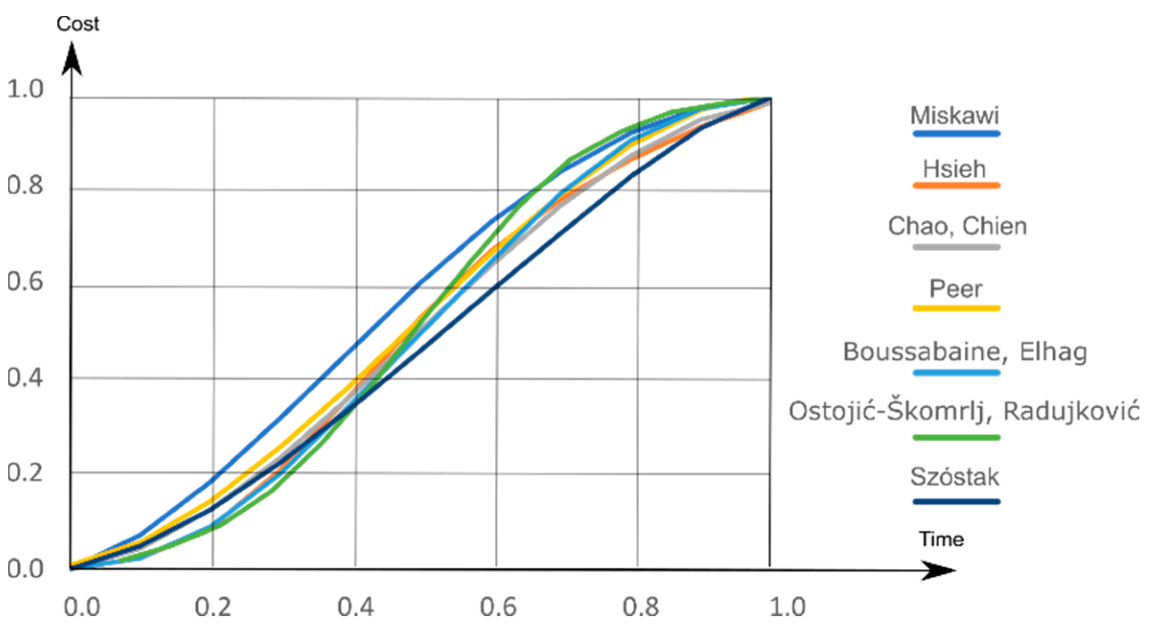
Figure 2 shows the graphs of the cost curves presented in Table 1 proposed by various researchers. A typical graph showing a cumulative cost/time analysis of a construction project is reduced to v = 100%, t = 100%. Variable Y represents the cumulative percentage of funds invested in construction, while variable X represents the cumulative percentage of time it takes to complete the construction process.

The traditional approach to cost forecasting usually uses a single model that reflects the entire course of actual construction projects. However, each construction project consists of different stages, which involve different costs, which are difficult to include in one model or mathematical formula [31]. Therefore, models have also been proposed in which three time periods are distinguished, which, according to the authors, allow you to plan and control costs with greater accuracy [32]. In each period of the construction phase, a properly adapted optimization and forecasting model is used to estimate the cost in a short period of time [33]. However, the main problem of the proposed method is to correctly identify the right moment during the transition from one phase to another and apply the actual slope coefficient of the curve, as well as the forecasting period in which the change in the coefficient occurs. For proper adjustment of the shape of the S-curve, it is important to correctly define the inflection point of the curve, i.e., to determine the moment in time when the curve changes from a convex to a concave curve. Unfortunately, during the planning of a construction project, as well as during the introduction of changes in the budget during the implementation of works, this point is difficult to determine, and sometimes even impossible to determine [34].

Comparing the mathematical formulas proposed by individual authors describing the shape of the cost curve, it should be noted their descriptions most often used:

• 6-degree polynomial [27,29,30];
• 3-degree polynomial [24,25,28];
• Less often, a 2-degree polynomial and a linear function [26].

The use of a 1-degree polynomial (linear function) and 2-degree (quadratic trinomial) is possible only on the assumption that the course of the investment process can be divided into a minimum of three periods. According to the literature on the subject, the cumulative cost graph is a curve with variable slopes and with a characteristic inflection point, i.e., the transition from a convex to concave function, which is why the use of a parabolic graph in the first and third periods is a large generalization. Analyzing the empirical graphs of cost curves proposed by other researchers, it is difficult to agree that in the second period the graph of the function takes a linear form. In addition, the correct, reflective of reality, division of duration into periods (e.g., three periods) is difficult to determine unambiguously, universally. Each investment venture is characterized by a different course, and incorrect division into periods can lead to making a significant mistake and obtaining an unreliable, unreal shape of the cost curve [32,35].

Therefore, to describe the course of the cost curve, it is reasonable to use only higher-order polynomials, minimum 3-degree. The use of the 6-degree polynomial trend allows to obtain a high value of the correlation coefficient (close to unity, indicating the occurrence of a very strong correlation relationship and a very good description of the studied phenomenon) and a low value of the coefficient of variation (indicating low variability of the characteristic and homogeneity of the studied population); its practical application may be difficult and complicated for decision-makers and can be considered inappropriate. From the practical point of view of the investor, contractor, or bidder, the use of polynomials of higher orders (higher than the 4-degree polynomial) may be difficult to apply. Therefore, simple mathematical formulas are being sought to correctly reproduce cost curves. Analysis of the literature of the subject indicates that the optimal formula is a 3-degree polynomial.

Based on a literature review, it was proven that research on the course of the cost curve is a very demanding task and the “search” for a universal solution is still ongoing [36].

On the basis of our own research, it was noted that the actual cost curve usually has a course similar to the course of the planned S-curve, but there are significant differences. The graphical shape of the theoretical cost curves is very regular, fluid, and continuous (as can be seen in Figure 2); while analyzing the actual course of empirical cost curves, it should be noted that their shape deviates significantly from the standard “S” curve.

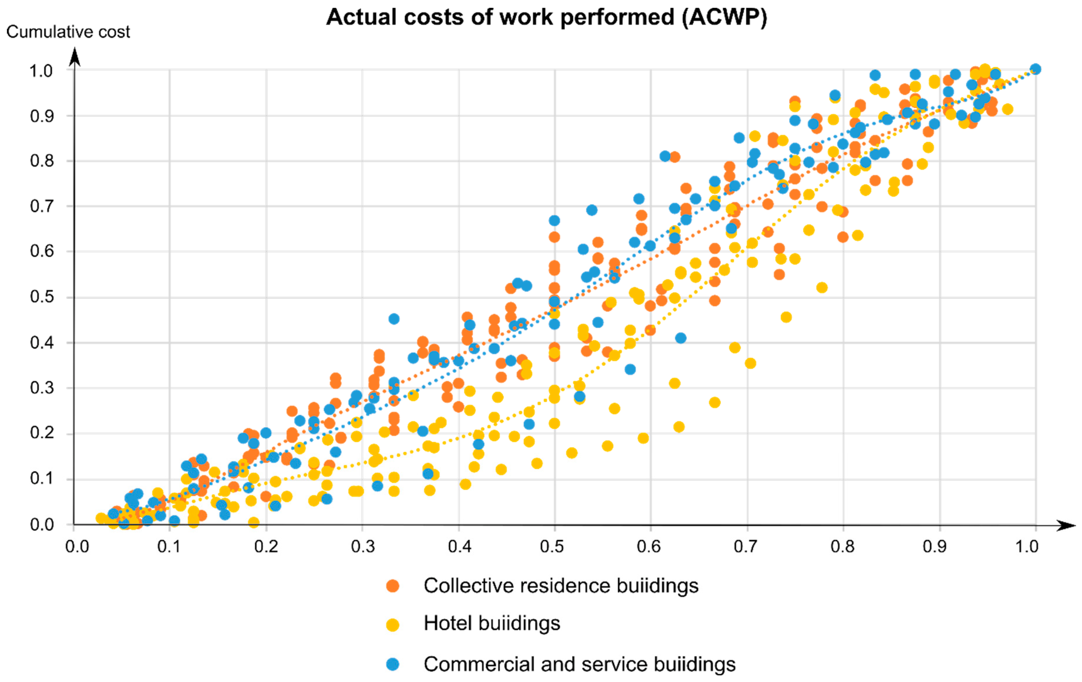
Analyzing the course of actual costs for an example of the analyzed investment project presented in Figure 3, one can notice differences between planned and developed cumulative costs, as well as downtime (horizontal part of the cost curve), resulting from the lack of actual financial processing. Therefore, when planning the course of the cost curve, it is advisable to use the space of cost curves rather than one model mathematical expression presented, for example, by a polynomial of the third or higher order. Cost curves, within a certain bounding box, determine the area of cash flows [37].

3. Method of Research

The study of the distribution of costs over time for selected groups of construction projects was carried out in accordance with the proposed original methodology of modeling cost curves “S” in order to determine the best fit curve and the space of cost curves, which, in the most appropriate way, present cost relations in typical conditions for the implementation of construction projects [12,30,38].

Two approaches were used to achieve the goal:

• Theoretical, resulting from the literature review carried out;
• Empirical, on the basis of collected own data on the course of actual construction projects.

Each of these approaches allows the development of several alternative curves, depending on the input. In a theoretical approach, all alternative proposals come from both the international and national literature. After becoming acquainted with the literature of the subject, works were selected that described cost curves using mathematical expressions, which are discussed in the literature review. In the second, empirical approach, cost curve modeling was carried out through a detailed analysis of the collected data on completed construction projects. In both approaches, the results of research and analysis are presented using mathematical formulas of the cumulative cost distribution and using an appropriate diagram.

In order to achieve the set goal of the research, it was necessary to obtain reliable and real data on each analyzed construction project, namely, to obtain a basic material and financial schedule and information on the actual course of the construction process. On the basis of the financial schedule of works, it is possible to graphically present the planned course of the cumulative cost curve, while on the basis of monthly summaries of construction works processing, containing percentage advancement and the value of works carried out in a given settlement period, it is possible to actually reconstruct the course of work implementation and develop a curve of actual cumulative costs.

This research collected data on 28 construction projects belonging to three research groups, corresponding to three diversified investment sectors, namely:

• Buildings of collective residence—11 investments (188 reports);
• Hotel buildings—9 investments (125 reports);
• Commercial and service buildings—8 investments (121 reports).

A total of 434 reports prepared by inspectors of banking supervision participating in the course of the analyzed construction projects were collected. All collected data concerned investments carried out in Poland in the period 2006–2020 present in

Table 2. Summary of the number of cumulative cost measurements in the BIS reports.

Construction Group/Sector	Amount	Measurement Period	PR	MR	FR
A. Building of collective residence	11	2006–2020	11	166	11
B. Hotel buildings	9	2013–2020	9	107	9
C. Commercial and service buildings	8	2008–2018	8	105	8
Total number of PR-MR-FR reports			28	378	28
Total number of all reports			434

PR: preliminary reports; MR: monthly reports; FR: final reports.

.

The research covered the time distribution of planned and actual cumulative capital expenditures and the trend of their adjustment to the literature S-curve. The course of the trend function was determined on the basis of the cumulative costs of the actual works performed. The analyzed data are reliable, consistent, and uniform. They can be used to isolate typological research samples for investments with a similar profile or for different construction sectors. Measurements of investment costs monitored in BIS reports, the number of which exceeds 100, can be additionally extrapolated to homogeneous populations.

As a result of the analysis of the reports, a summary of data in the form of a two-dimensional table in Microsoft Excel was developed, characterizing individual construction projects. In the table, each subsequent column contained data on subsequent reported periods, while in each subsequent row there were data on the next construction project. Each dataset contained the following values:

• The budgeted cost of the work scheduled for each individual period examined, determined on the basis of the basic of initial financial schedule of planned works;
• The actual cost of the work performed for each individual period examined, determined on the basis of monthly summaries of works carried out to date.

The collected data characterized individual construction projects. Since each project has a different duration and cost of implementation, in order to be able to compare the aggregated data for different construction projects, it was necessary to process the collected data accordingly. In order to carry out a comparative analysis, the data were normalized. Using the non-nominated values set for each project, it was possible to graphically present the collected data and develop charts showing:

• The budgeted cost of the work scheduled;
• The actual cost of the work performed.

Graphs were developed for each individual analyzed construction project and for homogeneous research groups, corresponding to three different investment sectors (A–C), and in a diverse group of different investment sectors.

Then, the best fit curves were determined in the form of a polynomial, with the best fit. To describe the course of curves, two approaches were used to determine the course of the curve using:

• Polynomial regression and trend function, in the form of a higher polynomial (5, 6) of the order;
• Polynomial of the third degree and the inflection point of the curve.

Based on the collected data, it was possible to determine the spaces of cost curves in which the best fit curves are located. In order to determine the space of cost curves, it was necessary to specify, for each analyzed dataset, the best fit curve, the curve limiting the space of cost curves “from the top”, and the curve limiting the space of cost curves “from the bottom”.

4. Research Results

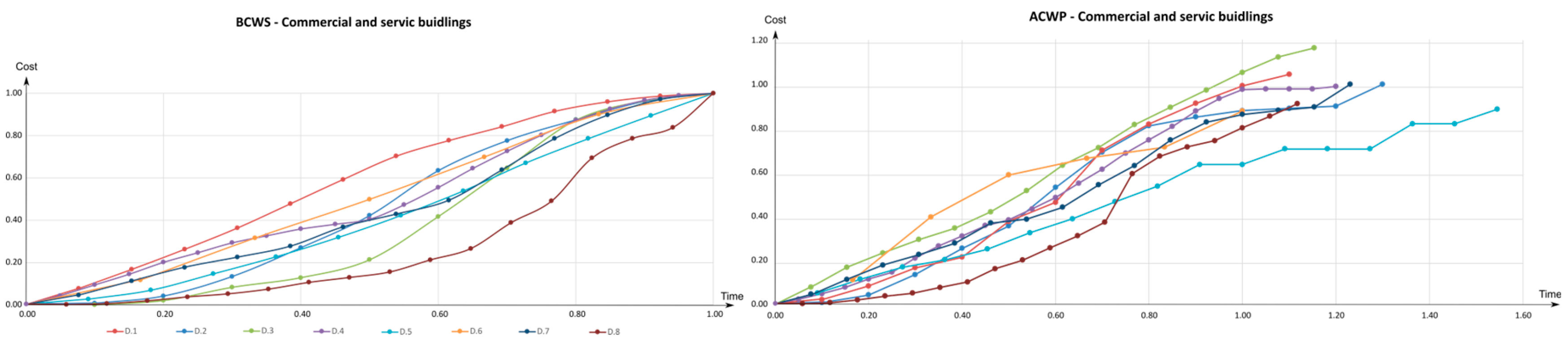
Figure 4 presents the obtained research results for the three analyzed research groups, corresponding to three different investment sectors: collective housing buildings, hotel buildings, and commercial and service buildings, for planned and real cost curves.

For the construction projects shown in Figure 4, belonging to three different sectors, the best matching curves in the form of a polynomial, with the best fit, were determined. Therefore, for polynomial regression and trend function, in the form of a higher-order polynomial, i.e., 6-degree, a correlation coefficient $R$and a coefficient of determination $R^2$ were used as a measure of the matching of the trend function to real values. The coefficient of determination $R^2$takes values between 0 and 1. The model match is better the closer the value is to unity. In this approach, a 6-degree polynomial was chosen, presented in

Table 3. A 6-degree polynomial describing the shape of the cost curve (best fit).

Research Group	6-Degree Polynomial
	Budgeted Cost of the Work Scheduled	Coefficient of Determination	Actual Cost of the Work Performed	Coefficient of Determination
Collective residence buildings (A.1–A.11)	y = −3.2249·x6 + 8.1654·x5 − 7.4172 ·x4 + 1.8996·x3 + 1.2183 x2 + 0.3604·x	R2 = 0.9798	y = −12.4030·x6 − 41.0300·x5 + 51.6030·x4 − 30.9180·x3 + 9.0692·x2 − 0.1288·x	R2 = 0.9542
Hotel buildings (B.1–B.9)	y = −5.3155·x6 + 2.0428·x5 + 12.0040 x4 − 11.4940 x3 + 3.7482 x2 + 0.0096·x	R2 = 0.9434	y = 21.3330·x6 − 65.4280·x5 + 71.1750·x4 − 32.5880·x3 + 6.5248·x2 − 0.1179·x	R2 = 0.9349
Commercial and service buildings (C.1–C.8)	y = 13.7870 x6 -45.2590 x5 + 53.508 x4 − 27.96 x3 + 6.9312 x2 − 0.0101 x	R2 = 0.8964	y = 20.2120·x6 − 55.798·x5 + 55.5240·x4 − 24.9370·x3 + 5.8078·x2 + 0.1908·x	R2 = 0.9450
All buildings (A.1–C.8)	y = 0.0267 x6 − 76.7050·x5 + 14.0970·x − 10.0460·x3 + 3.4796 x2 + 01463 x	R2 = 0.9102	y = 17.6170·x6 − 53.6520·x5 + 59.7800·x4 − 30.0750·x3 + 7.3388·x2 − 0.0099·x	R2 = 0.9176

, which allows to obtain a value of the correlation coefficient $R$ close to unity and high accuracy.

Unfortunately, the use of a polynomial of such a high degree is problematic, because there are a large number of variables, and the resulting polynomial is of little use.

Based on the analysis of the literature on the subject and the shape of cost curves, it was noticed that cost curves resemble the shape of the letter “S”. The letter “S” from a mathematical point of view has two convexness (and one inflection point $x_0$, as shown in Figure 5.

Traditional cost curves are as follows:

• In the first period of execution of works (phase one), the cost curves are convex—from a geometric point of view, this means that the graph of the function lies above the tangent graph for each point in the interval $<0,x_0)$; function graph arc connecting any two points ($A,B$) from the interval $<0,x_0)$ of this graph lies below or on the chord connecting the points ($A,B$).

• During the increased implementation of construction works, increasing progress of works, and the passage of time, it can be noticed that in the central part, the cost curve is steep, i.e., inclined at a large angle in relation to the timeline.
• The cost curve at some point in the execution of construction works reaches the inflection point ($x_0$) informing about the moment of transition of the investment to the second phase of implementation, in which the cost increase begins to slow down.

• In the second phase of the works, the cost curve is concave, i.e., convex upwards (from a geometric point of view, this means that the graph of the function lies under the tangent graph for each point in the interval $(x_0,1>$; function graph arc connecting any two points ($C,D$) from the interval $(x_0,1>$ of this graph lies above or on the chord connecting the points ($C,D$).

Adopting this approach allowed the use of a polynomial of the third degree with the following equation:

$$f\left(x\right)=a_1·x^3+a_2·x^2+a_3·x^1+a_0$$

(1)

where variables $x,y$ denote normalized cost progress and standardized project duration, while variables: $a_1$, $a_2$, and $a_3$ are the parameters to be specified. To determine variables, it is assumed that:

• The axis of the severed takes values from 0 to 1 (the range is closed on both sides): $x\in \langle 0,1\rangle$.

• The ordinate axis takes values from 0 to 1 (the range is closed on both sides): $y\in \langle 0,1\rangle$.

• The cost curve begins at a point with coordinates (0.0), which means that the free word is 0: $a_0=0$.

• Polynomial for $x=1$ always takes a value of 1 for the completed investment ($y=1$): $f\left(1\right)=1=a_1·x^3+a_2·x^2+a_3·x$, and this means that: $a_1+a_2+a_3=1$.

• A polynomial of the third degree has at most one inflection point. In order to determine the inflection point, the necessary condition must be met, which is the zeroing of the second derivative of the function: $f^{″}\left(x\right)=0$:

$$f^{\prime }\left(x\right)=3·a_1·x^2+2·a_2·x+a_3$$

(2)

$$f^{″}\left(x\right)=6·a_1·x+2·a_2=0$$

(3)

• We obtain an inflection point: $x_0=\frac{-a_2}{3·a_1}$.

• The polynomial (cost curve) can be characterized by the inflection point ($x_0$) informing about the moment of transition of the investment to the “second phase”.

Based on the polynomial of the third degree and the inflection point, for each dataset, it was possible to determine the curves of the best fit. The resulting polynomials are shown in

Table 4. A 3-degree polynomial describing the shape of the cost curve (best fit).

Research Group	3-Degree Polynomial
	Budgeted Cost of the Work Scheduled	Coefficient of Determination	Inflection Point	Actual Cost of the Work Performed	Coefficient of Determination	Inflection Point
Collective residence buildings (A.1–A.11)	y = −1.04 x3 + 1.72 ·x2 + 0.32·x	R2 = 0.9797	x = 0.5513	y = −0.57 x3 + 0.94 x2 + 0.63·x	R2 = 0.9535	x = 0.5497
Hotel buildings (B.1–B.9)	y = −0.60·x3 + 1.59 ·x2 + 0.01·x	R2 = 0.9325	x = 0.8833	y = −0.65·x3 + 1.71 ·x2 − 0.06·x	R2 = 0.9279	x = 0.8769
Commercial and service buildings (C.1–C.8)	y = −0.77 x3 + 1.56 ·x2 + 0.21·x	R2 = 0.9532	x = 0.6752	y = −1.30·x3 + 1.99 ·x2 + 0.31·x	R2 = 0.9438	x = 0.5103
All buildings (A.1–C.8)	y = −0.67 x3 + 1.36 ·x2 + 0.31·x	R2 = 0.9172	x =0.6766	y = −0.78·x3 + 1.49 ·x2 + 0.29·x	R2 = 0.9162	x = 0.6368

. As a measure of matching the function to the actual values, the correlation coefficient $R$ described earlier was used, and coefficient of determination $R^2$.

Figure 6 and Figure 7 show the best fit curves for the obtained 3-degree polynomials together with the resulting cost curve spaces for the three analyzed research groups for the planned and actual cost curves.

Table 5. Cost curve envelope.

Research Group	The Actual Cost Curve of the Border “From the top”	Actual Best Fit Curve	The Actual Cost Curve of the Border “From the Bottom”
Collective residence buildings (A.1–A.11)	y = −1.06 x3 + 1.19 x2 + 0.87 x	y = −1.04 x3 + 1.72 x2 + 0.32 x	y = 0.09 x3 + 0.54 x2 + 0.37 x
Hotel buildings (B.1–B.9)	y = −1.20 x3 + 2.01 x2 + 0.19 x	y = −0.60 x3 + 1.59 x2 + 0.01 x	y = 0.94 x3 + 0.04 x2 + 0.02 x
Commercial and service buildings (C.1–C.8)	y = −1.30 x3 + 1.99 x2 + 0.31 x	y = −0.77 x3 + 1.56 x2 + 0.21 x	y = 0.94 x3 + 2.34 x2 − 0.40 x
All buildings (A.1–C.8)	y = −1.20 x3 + 1.40 x2 + 0.82 x	y = −0.67 x3 + 1.36 x2 + 0.31 x	y = 0.86 x3 + 0.10 x2 + 0.04 x

provides a mathematical record of the resulting curves forming banana envelopes of cost curves (the banana envelope of the S-curve).

5. Discussion

5.1. Summary

Knowledge of the planned course of accumulated financial outlays in time and the actual shape of the S-curve and its deviations allows for rational action aimed at achieving the intended goal and success in the implementation of the construction project [39]. The decision-maker, having a specific budget of the investment and a certain duration of its duration, using the cost curve of the best fit, has the opportunity to properly plan financial flows over time [40].

Previous studies and analyses of standardized cost curves are based on data from previously completed projects [41]. This approach has been met with a lot of criticism, mainly due to the availability of reliable data. The availability of detailed data and their quality depend on the degree of planning of each project, that is, on whether a detailed schedule and individual assessments are part of the plan or not. It happens that detailed data are not available, and their quality and quantity are insufficient for the correct assessment of the investment project. It happens that no data are available for the project, so mathematical models have also been developed that can be used even in cases where little is known about the project [42]. Project data are sometimes limited only to information about type of project, i.e., investment sector (e.g., design of a collective residence building, design of an office building, design of a hotel building, design of a health center, etc.), construction technology (e.g., traditional technology–masonry, monolithic technology, prefabricated technology, steel construction technology, etc.), duration of the project, and the budget, i.e., the planned total costs [43].

The S-curve method, thanks to the conducted research, underwent constant modifications. For example, the theory of fuzzy sets was used to determine the shape of cost curves [44], using least squares and fuzzy regression method [45], artificial intelligence technique [46,47], as well as the use of elements of BIM technology in the field of automatic integration of the BIM-5D model with the schedule and costs [48,49]. The traditional method of generating cost curves was also extended to include elements that take into account risk analysis, which made it possible to determine the space of cost curves [50] and determining the impact of key causes of delays on the course of the cost curve in the risk conditions of construction projects [51].

Unexpected changes, uncertainty, or imprecision of the prepared data are a phenomenon inherent in the management of cost flows [52,53]. The use of a fuzzy stochastic model provides decision-makers with greater protection than deterministic planning methods against unexpected changes in cash flow in the investment budget. It is possible to take this phenomenon into account only with the use of modeling using probability theory. Therefore, an alternative to deterministic and forecasting deterministic and traditional cost curves is a simulation approach based on stochastic cost curves and on the variability of the duration and cost of individual tasks [54,55], and probabilistic approach using Bayesian models [56] and other probability distributions known in the literature [57,58].

In the conducted research, empirical methods of estimating the course of cost curves incremental in various construction projects were also used [59]. The obtained mathematical formulas of cost curves are based on real, historical data concerning, for example, construction projects carried out in Great Britain (in office, service, residential, and other buildings) [60], in Iran [61], in the United States [62], and in Poland [63].

As can be seen in subsequent modifications of the cumulative cost curve method, more and more complicated methods are used (fuzzy set theory, artificial intelligence, stochastics, probabilistic) and formulas that are difficult to apply [64]. In light of the above considerations, it is quite clear that end users, decision-makers, and investors require a simpler and faster approach, which is why complex models and mathematical formulas describing the course of curves have not met with much response and application.

Therefore, in the conducted research, it was decided to use a 3-degree polynomial. The degree of polynomial results from the conducted literature review and my own research.

5.2. Conclusions

The basic material and financial schedules developed by investors before the commencement of works and their own monthly results of measurements of incurred and developed costs/processing of construction works were subjected to research. An assessment of the actual costs incurred of investment tasks was carried out, the trend for which the cumulative cash flow curves can be estimated with a large match by forecasting the construction process. The spaces of the S-curves of the planned costs were determined with third-degree polynomials for three research groups, corresponding to diverse investment sectors: collective residence buildings, hotel buildings, and commercial and service buildings.

On the basis of the analyses and studies carried out, the following conclusions were drawn:

• The planned cost curves proposed so far in the literature are not reflected in reality. The actual course of the cost curves is more irregular and deviates significantly from the reference “S” curve.
• Cost curves, within a certain bounding box, determine the area of the most likely cash flow.
• When planning the course of a cost curve, it is advisable to use the bounding box of cost curves rather than a single, model, theoretical, or empirical mathematical expression describing the cost curve.
• For actual cost curves, the inflection point of the curve occurs earlier than for the planned cost curves. This means that despite the longer implementation time, there is a moment earlier during the investment project in which the curve changes from convex to concave. From this point on, the pace of work slows down.
• As part of the research, an attempt was made to describe the course of cost curves using mathematical relationships between variable parameters, i.e., time and cost.

The research works on the best fit of cumulative cost curves at the planning and performed stages of construction projects are still open and ongoing. The data of the period 2021–2022 were collected so as to supplement presented findings on courses of cumulative cost curves (CCCC) that represent the state of the art in financial construction management.

References

- Gupta, C.; Kumar, C. Study of factors causing cost and time overrun in construction projects. Int. J. Eng. Res. Technol. 2020, 9, 202–206. [Google Scholar]
- Amade, B.; Akpan, E. Project cost estimation: Issues and the possible solutions. Int. J. Eng. Tech. Res. 2014, 2, 181–188. [Google Scholar]
- Kerzner, H. Project Management: A Systems Approach to Planning, Scheduling, and Controlling; John Wiley & Sons, Inc.: New York, NY, USA, 2003. [Google Scholar]
- Fazil, M.; Lee, C.; Tamyez, P. Cost estimation performance in the construction projects: A systematic review and future directions. Int. J. Ind. Eng. Manag. 2021, 11, 217–234. [Google Scholar] [CrossRef]
- Milat, M.; Knezić, J.; Sedlar, J. Resilient Scheduling as a Response to Uncertainty in Construction Project. Appl. Sci. 2021, 11, 6493. [Google Scholar] [CrossRef]
- Plebankiewicz, E.; Zima, K.; Wieczorek, D. Modelling of time, cost and risk of construction with using fuzzy logic. J. Civ. Eng. Manag. 2021, 27, 412–426. [Google Scholar] [CrossRef]
- Leśniak, A.; Zima, K. Cost Calculation of Construction Projects Including Sustainability Factors Using the Case Based Reasoning (CBR) Method. Sustainability 2018, 10, 1608. [Google Scholar] [CrossRef] [Green Version]
- Grzyl, B.; Apollo, M.; Miszewska-Urbaska, E.; Kristowski, A. Management of exploitation in terms of life cycle costs of built structures. Acta Sci. Pol. Archit. 2017, 16, 85–89. [Google Scholar]
- Połoński, M. Forecasting civil structure duration on the basis of progress of works. Quant. Methods Econ. 2012, 13, 169–179. [Google Scholar]
- Shinde, M.; Mata, M. Financial planning in construction project. Int. Res. J. Eng. Technol. 2016, 3, 2702–2709. [Google Scholar]
- Zin, R.; Mohamad, M.; Mansur, S.; Tee, D. Guidelines for the preparation and submission of work schedule for construction project. Malays. J. Civ. Eng. 2008, 20, 145–159. [Google Scholar]
- Konior, J. Determining Cost and Time Performance Indexes for Diversified Investment Tasks. Buildings 2022, 12, 1198. [Google Scholar] [CrossRef]
- Szafranko, E.; Harasymiuk, J. Modelling of decision processes in construction activity. Appl. Sci. 2022, 12, 3797. [Google Scholar] [CrossRef]
- Kasprowicz, T.; Starczyk-kołbyk, A.; Wójcik, R. Randomized Estimation of the Net Present Value of a Residential Housing Development. Appl. Sci. 2022, 12, 124. [Google Scholar] [CrossRef]
- Połoński, M. Application of the work breakdown structure in determining cost buffers in construction schedules. Arch. Civ. Eng. 2015, 61, 147–161. [Google Scholar] [CrossRef] [Green Version]
- Konior, J.; Szóstak, M. Cumulative cost spent on construction projects of different sectors. Civ. Eng. Archit. 2021, 9, 999–1011. [Google Scholar] [CrossRef]
- Miguel, A.; Madria, W.; Polancor, R. Project management model: Integrating Earned Schedule, quality, and risk in Earned Value Management. In Proceedings of the 6th IEEE International Conference on Industrial Engineering and Applications (ICIEA), Waseda, Tokyo, 12–15 April 2019; pp. 622–628. [Google Scholar]
- Guan, X.; Servranckx, T.; Vanhoucke, M. An analytical model for budget allocation in risk prevention and risk protection. Comput. Ind. Eng. 2021, 161, 107657. [Google Scholar] [CrossRef]
- Starczyk-Kołbyk, A.; Kruszka, L. Use of the EVM method for analysis of extending the construction project duration as a result of realization disturbances—Case study. Arch. Civ. Eng. 2021, 67, 373–393. [Google Scholar]
- Duarte-Vidal, L.; Herrera, R.; Atencio, E.; Muñoz-La Rivera, F. Interoperability of digital tools for the monitoring and control of construction projects. Appl. Sci. 2021, 11, 10370. [Google Scholar] [CrossRef]
- Salari, M.; Khamooshi, H. A better project performance prediction model using fuzzy time series and data envelopment analysis. J. Oper. Res. Soc. 2016, 67, 1274–1287. [Google Scholar] [CrossRef]
- Hajali-Mohamad, M.; Mosavi, M.; Shahanaghi, L. Optimal estimating the project completion time and diagnosing the fault in the project. DYNA 2016, 83, 121–127. [Google Scholar] [CrossRef]
- Tijanić, K.; Car-Pušić, D. Application of S-curve in EVA Method. In Proceedings of the 13th International Conference Organization, Technology and Management in Construction, Zagreb, Croatia, 27–30 September 2017; pp. 103–115. [Google Scholar]
- Peer, S. Application of cost-flow forecasting models. J. Constr. Div. 1982, 108, 226–232. [Google Scholar] [CrossRef]
- Miskawi, Z. An S-curve equation for project control. Constr. Manag. Econ. 1989, 7, 115–124. [Google Scholar] [CrossRef]
- Boussabaine, A.; Elhag, T. Applying fuzzy techniques to cash flow analysis. Constr. Manag. Econ. 1999, 177, 745–755. [Google Scholar] [CrossRef]
- Hsieh, T.Y.; Wang, M.H.L.; Chen, C.W. A Case Study of S-Curve Regression Method to Project Control of Construction Management via T-S Fuzzy Model. J. Mar. Sci. Technol. 2004, 12, 209–216. [Google Scholar] [CrossRef]
- Chao, L.; Chien, C. Estimating project S-curves using polynomial function and neural networks. J. Constr. Eng. Manag. 2009, 135, 169–177. [Google Scholar] [CrossRef]
- Ostojic-Skomrlj, N.; Radujkovic, M. S-curve modelling in early phases of construction projects. Gradevinar 2012, 64, 647–654. [Google Scholar]
- Szóstak, M. Planning the time and cost of implementing construction projects using an example of residential buildings. Arch. Civ. Eng. 2021, 67, 243–259. [Google Scholar]
- Soliman, E.; Alrasheed, K. Difference in S-curve for different types of construction projects. J. Eng. Res. 2021, 10, 17–28. [Google Scholar] [CrossRef]
- Cioffi, D. A tool for managing projects: An analytic parameterization of the S-curve. Int. J. Proj. Manag. 2005, 23, 215–222. [Google Scholar] [CrossRef]
- Cheng, Y.; Yu, C.; Wang, H. Short-interval dynamic forecasting for actual S-curve in the construction phase. J. Constr. Eng. Manag. 2011, 137, 933–941. [Google Scholar] [CrossRef]
- Kozień, E. Application of approximation technique to on-line updating of the actual cost curve in the earned value method. Czas. Tech. 2017, 9, 181–195. [Google Scholar]
- Rashid, H.; Al-juboori, O.; Mahjoob, A. New cost control techniques in mega construction projects. Period. Eng. Nat. Sci. (PEN) 2021, 9, 454–461. [Google Scholar] [CrossRef]
- Hwang, B.-G.; Shan, M.; Zhu, L.; Lim, W.-C. Cost control in megaprojects: Efficacy, tools and techniques, key knowledge areas and project comparisions. Int. J. Constr. Manag. 2018, 20, 437–449. [Google Scholar] [CrossRef]
- Cheng, M.; Tsai, H.; Liu, C. Artificial intelligence approaches to achieve strategic control over project cash flows. Autom. Constr. 2009, 18, 386–393. [Google Scholar] [CrossRef]
- Konior, J.; Szóstak, M. Methodology of planning the course of the cumulative cost curve in construction projects. Sustainability 2020, 12, 2347. [Google Scholar] [CrossRef] [Green Version]
- Przywara, D.; Rak, A. Monitoring of time and cost variances of schedule using bullet earned value method indicators. Appl. Sci. 2021, 11, 1357. [Google Scholar] [CrossRef]
- Tembo, C.; Muleya, F.; Kanyemba, A. An appraisal of cost management techniques used in the construction industry. Int. J. Constr. Manag. 2022, 1–9. [Google Scholar] [CrossRef]
- Araujo-Rey, C.; Sesastian, M. An Approach to the analysis of causes of delays in industrial construction projects through planning and statistical computing. Sustainability 2021, 13, 3975. [Google Scholar] [CrossRef]
- Mardiaman, M.; Kusuma, E. Study of progress expected results based on percentage of construction work plan duration. Civ. J. Tek. Sipil Univ. Islam Lamongan 2021, 6, 167–180. [Google Scholar] [CrossRef]
- Servranckx, T.; Vanhoucke, M.; Aouam, T. Practical application of reference class forecasting for cost and time estmiations: Identifying the properties of similarity. Eur. J. Oper. Res. 2021, 295, 1161–1179. [Google Scholar] [CrossRef]
- Mohagheghi, V.; Meysam Mousavi, S.; Vahdani, B. An assessment method for project cash flow under interval-valued fuzzy environment. J. Optim. Ind. Eng. 2017, 22, 79–80. [Google Scholar]
- Hsieh, T.; Wang, M.; Chen, C.; Chen, C.; Yu, S.; Yang, H.; Chen, H. A new viewpoint of s-curve regression model and its application to construction management. Int. J. Artif. Intell. Tools 2006, 15, 131–142. [Google Scholar] [CrossRef]
- Chao, L.; Chien, C. A model for updating project S-curve by using neural networks and matching progress. Autom. Constr. 2010, 19, 84–91. [Google Scholar] [CrossRef]
- Chao, L.; Chen, H. Predicting project progress via estimation of S-curve’s key geometric feature values. Autom. Constr. 2015, 57, 33–41. [Google Scholar] [CrossRef]
- Wang, K.; Wang, W.; Wang, H.; Hsu, P.; Wu, W.; Kung, C. Applying building information modeling to integrate schedule and cost for establishing construction progress curves. Autom. Constr. 2016, 72, 397–410. [Google Scholar] [CrossRef]
- Atencio, E.; Araya, P.; Oyarce, F.; Herrera, R.; Muñoz-La Rivera, F.; Lozano-Galant, F. Towards the Integration and Automation of the Design Process for Domestic Drinking-Water and Sewerage Systems with BIM. Appl. Sci. 2022, 12, 9063. [Google Scholar] [CrossRef]
- Maravas, A.; Pantouvakis, J. Project cash flow analysis in the presence of uncertainty in activity duration and cost. Int. J. Proj. Manag. 2012, 30, 374–384. [Google Scholar] [CrossRef]
- Mohamad, H.; Mohamad, M.; Saad, I.; Bolong, N.; Mustazama, J.; Razali, S. A case study of s-curve analysis: Causes, effects, tracing and monitoring project extension of time. Civ. Eng. J. 2021, 7, 649–661. [Google Scholar] [CrossRef]
- Anysz, H.; Rosłon, J.; Foremny, A. 7-Score Function for Assessing the Strength of Association Rules Applied for Construction Risk Quantifying. Appl. Sci. 2022, 12, 844. [Google Scholar] [CrossRef]
- Jafari, P.; Hattab, M.; Mohamed, E.; Abourizk, S. Automated Extraction and Time-Cost Prediction of Contractual Reporting Requirements in Construction Using Natural Language Processing and Simulation. Appl. Sci. 2021, 11, 6188. [Google Scholar] [CrossRef]
- Barraza, G.; Back, W.; Mata, F. Probabilistic forecasting of project performance using stochastic S curves. J. Constr. Eng. Manag. 2004, 130, 25–32. [Google Scholar] [CrossRef]
- Yao, J.; Chen, M.; Lu, H. A fuzzy stochastic single-period model for cash management. Eur. J. Oper. Res. 2006, 170, 72–90. [Google Scholar] [CrossRef]
- Kim, B.; Reinschmidt, K. An S-curve Bayesian model for forecasting probability distributions on project duration and cost at completion. Eng. Mater. Sci. 2007, 1449–1459. [Google Scholar]
- Kim, B.; Reinschmidt, K. Probabilistic forecasting of project duration using Bayesian inference and the beta distribution. J. Constr. Eng. Manag. 2009, 135, 178–186. [Google Scholar] [CrossRef]
- Sobieraj, J.; Metelski, D. Project Risk in the Context of Construction Schedules—Combined Monte Carlo Simulation and Time at Risk (TaR) Approach: Insights from the Fort Bema Housing Estate Complex. Appl. Sci. 2022, 12, 1044. [Google Scholar] [CrossRef]
- Martens, A.; Vanhoucke, M. Integrating corrective actions in project time forecasting using exponential smoothing. J. Manag. Eng. 2020, 36, 1–34. [Google Scholar] [CrossRef]
- Blyth, K.; Kaka, A. A novel multiple linear regression model for forecasting S-curves. Eng. Constr. Archit. Manag. 2006, 13, 82–95. [Google Scholar] [CrossRef] [Green Version]
- Banki, M.; Esmaeeli, B. Using historical data for forecasting s-curves at construction industry. In Proceedings of the IEEE International Conference on Industrial Engineering and Engineering Management, Singapore, 08–11 December 2008; pp. 282–286. [Google Scholar]
- Jiang, A.; Issa, R.; Malek, M. Construction project cash flow planning using the Pareto optimality efficiency network model. J. Civ. Eng. Manag. 2011, 17, 510–519. [Google Scholar] [CrossRef] [Green Version]
- Konior, J.; Szóstak, M. The S-curve as a tool for planning and controlling of construction process-case study. Appl. Sci. 2020, 10, 2071. [Google Scholar] [CrossRef] [Green Version]
- Yaseen, Z.; Ali, Z.; Salih, S.; Al-Ansari, N. Prediction of risk delay in construction projects using a hybrid artificial intelligence model. Sustainability 2020, 12, 1514. [Google Scholar] [CrossRef]
Figure 1.
Model of cumulative cost curve.
Figure 2.
Cost curve graphs proposed by individual researchers.
Figure 3.
Graph of theoretical and actual cost curve.
Figure 4.
Graph cumulative cost curves.
Figure 5.
Cost curve with inflection point.
Figure 6.
Best fit 3-degree curves and curve spaces for budgeted costs of work scheduled.
Figure 7.
Best fit 3-degree curves and curve spaces for actual cost of work performed.