1. Introduction
Project management is a systematic approach that involves planning, organizing, directing, and controlling a project to accomplish certain specific objectives [
1]. Its objective is to achieve the dynamic management of the entire project process [
2]. In the 1960s, project management was confined to a few areas such as defenses, aerospace and construction engineering [
3]. The success of project management in the implementation of a wide range of major projects has made it a global phenomenon. At present, project management is used in a wide range of fields such as software engineering, network communications, the financial industry and even government agencies [
4].
With the accelerated pace of society and rapid economic growth, it has always been a common goal to create as much value as possible in the shortest possible time [
5]. For builders, a higher production efficiency may mean lower production costs or shorter construction lead times [
6]. Production costs are constrained by a number of factors such as policy, market, capital and quality, and there is very limited scope for reduction [
7]. Various factors need to be taken into account when compiling the construction schedule [
8], and there is more room to maneuver in these factors. As a result, shortening the construction cycle has become an important way to increase productivity.
In practice, there is a problem in shortening the construction cycle. The process of compiling a construction schedule requires an estimate of the duration of the work. Managers usually include a significant amount of safety time to ensure that projects are completed on time, taking into account the uncertainties and potential risks. However, this inclusion of a large amount of safety time tends to accumulate due to deviations and is not conducive to project schedule control, leading to slack between processes and ultimately delays [
9]. Although traditional project management techniques have proven to be effective tools for project management, such as the Critical Path Method (CPM) [
10] and the Program Evaluation and Review Technique (PERT) [
11], these methods are also unable to deal with the situation.
In 1997, Dr. Goldratt, the originator of the Theory of Constraints (TOC), published his book “Critical Chain”. In the book, he introduced TOC to project management [
12]. A new approach to project management, Critical Chain Project Management (CCPM), is proposed. By inserting buffers into the project schedule, CCPM ensures that the project will run smoothly and on schedule by absorbing the uncertainty of the project through properly set buffers [
13,
14,
15]. The application of CCPM to project management can significantly improve project performance and there are many examples of successful applications [
16]. For example, critical chains are introduced into the turnaround process for IGCC (Integrated Gasification Combined Cycle) plants to minimize the risks associated with refinery accidents [
17].There are also practical examples of the application of critical chains to the problem of scheduling resources for multiple projects in the automotive development process [
18]. Therefore, experts and scholars have developed a variety of models and calculation methods around project critical chain project management [
9]. A central unsolved problem within CCPM is the sizing of buffers, which is the focus of our work.
Accurate buffer calculations are essential for the control of project economics and schedules. Buffer sizes too small can lead to replanning, whereas too large a buffer zone could easily lead to a lack of competitiveness and potential economic loss. As a result, a wide variety of calculation methods and models have been proposed in the literature. Improvements to the current buffer setting have had some effect [
19], but there are still some problems. Our work focuses on the following two questions:
When considering the uncertainty calculation buffer for the duration of each activity, it is divided into multiple target factors for study. However, the correlation between the various target factors is present and creates a new uncertainty on the duration.
Buffers are designed to eliminate schedule risk, which arises from risk factors causing risk incidents. However, most studies have analyzed and quantified various uncertainty factors in terms of project attributes. Few studies have been conducted to calculate buffer sizes from a system perspective.
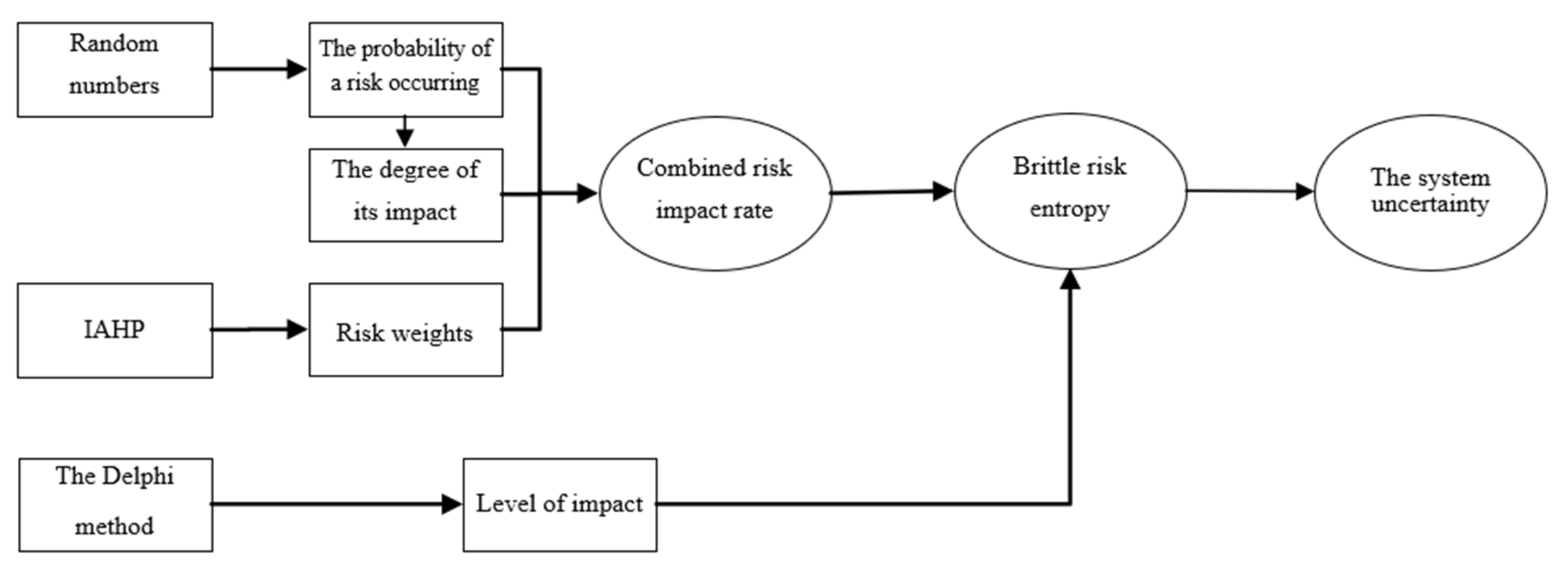
To address these issues, the article introduces the concept of integrated risk impact rate based on the analysis of the brittleness of the construction process, constructs a brittle risk entropy function for the project construction process from the dimension of the system, and measures the system uncertainty through the brittle risk entropy, avoiding the original singularity of starting from only one factor. The specific flow chart of the method is detailed in
Figure 1.
The remainder of this paper is organized as follows.
Section 2 reviews the relevant literature.
Section 3 focuses on the analysis of brittleness during construction.
Section 4 constructs the brittle risk entropy function on the basis of
Section 3.
Section 5 describes our buffer adjustment method.
Section 6 is an application of the method to a specific project for example analysis.
Section 7 presents some conclusions and suggestions for future work.
2. Literature Review
The most classical methods for calculating buffer size are the Cut-and-Paste Method (C&PM) [
12] proposed by Goldratt and the Root Square Error Method (RSEM) [
20] proposed by Newbold based on the Central Limit Theorem. Although the cut-and-paste method (C&PM) is simple and easy to calculate, a linear increase in buffer size occurs as the length of the work chain increases. The Root Square Error Method (RSEM) calculation is more reasonable and does not result in a buffer that is too large or too small, but it is premised on the assumption that the various processes of the project are executed independently of each other, which does not correspond to the reality of the project.
In addition, the calculation of buffers has been studied in depth by many scholars, with most methods improving on the limitations of the above two methods. Tukel et al. [
21] incorporated a calculation of the project buffer by analyzing the factors affecting the various processes in the project, taking into account the impact of resource constraints and the complexity of the project network. Zhang Junguang et al. [
22] integrated the physical resource tension with the information resource tension and proposed a buffer zone calculation method based on the integrated resource tension. Ghoddousi [
23] considered the influencing factors such as network complexity, activity rules, and criticality rules in order to maximize the robustness of buffer scheduling, and used simulations to justify the model. Based on Z-number theory, Zhao [
24] proposed a buffer calculation method that takes into account internal process risk, external project risk, and resource risk. Gong Jun et al. [
25] used complexity entropy, resource entropy and human factor entropy to measure uncertainty, while fully considering the impact of human behavioral factors on a project’s schedule as a way to set up critical chain buffers. Zhang J.G. [
26] developed a quantitative model for the determination of the optimal time window for resource buffering, considering factors such as bottleneck resource sensitivity, idle costs, start-up time flexibility and workflow in critical chains. Sarkar [
16] proposes an enhanced Critical Chain Project Management (CCPM) framework by integrating the various uncertainties affecting construction scheduling to improve buffer sizes.
At the same time, a number of scholars have also proposed new rules for calculating buffers, going beyond the limitations of the original the Cut-and-Paste Method (C&PM) and the Root Square Error Method (RSEM), and exploring the calculation of buffers from a wider range of dimensions. Bie [
27] analyzed the impact of inter-activity dependencies on project duration performance by integrating the two definitions of dependency and dependency factors, which reflect dependency, into a buffer size approach. Farag [
28] proposed a method for calculating buffer zones for construction projects based on fuzzy theory, taking into account the characteristics of the process and its degree of uncertainty. Leng Kaijun [
29] proposed a new method for buffer size adjustment using Bayesian networks, considering the risk of activity duration and the risk of multiple resource constraints under uncertainty. Seyed Ashkan et al. [
30] proposed project resource reliability analysis to obtain a probability metric that redefines the source of the buffer by using the availability of resources as a random variable for project scheduling. Roghanian [
31] introduced a new approach to buffer sizing based on the square and root-square (SSQ) method, taking into account resource constraints and other constraints, using the Resource-Constrained Project Scheduling Problem (RCPSP) model. Bingling She et al. [
32] proposed a new method for calculating the buffer size by comparing the incoming chain with a parallel critical chain, while later incorporating the degree of safety beyond the critical chain.
3. Analysis of Brittleness during Construction
As the system evolves and grows in size and number, the interconnections between the constituent elements within the system become more and more intertwined. When a part of a complex system is disturbed by internal or external factors and then fails, it passes down the chain of relationships, causing other parts to be affected, directly or indirectly affecting the whole system and eventually leading to its collapse. This property is known as the brittleness of complex systems [
33].
The brittleness of complex systems is characterized by the following.
Hiddenness. Brittleness does not manifest itself under normal circumstances. It only becomes apparent when a part of a complex system is disturbed by external factors.
Variety. As the brittleness is excited in different times, locations and states, the final manifestation and degree of brittleness also vary.
Harmfulness. The first manifestation of brittleness in a subsystem is the disturbance of the links, which reduces the operational efficiency of the whole system.
Chainability. When the brittleness of a subsystem is triggered, it will first cause fluctuations in the normal operation of one subsystem, further spreading to other subsystems and eventually leading to the collapse of the whole system.
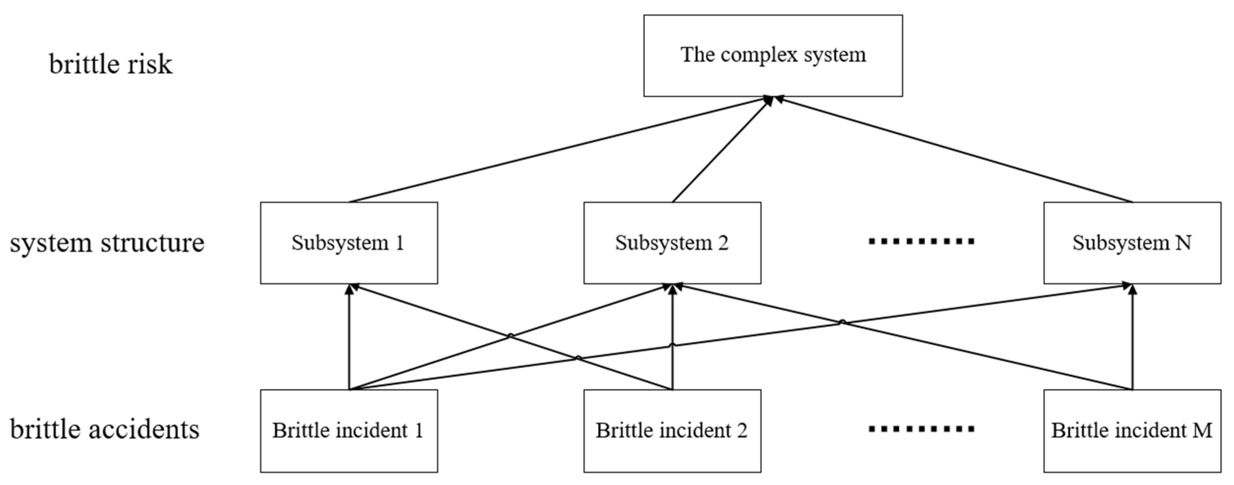
As a system of engineering involving different kinds of people, materials and machinery, construction projects are complex. We can assume that construction projects are also brittle and have the characteristics described above. In addition, we propose that the brittle structure of complex systems can be classified as brittle risk (system collapse), system structure, brittle accidents, etc. [
34] (
Figure 2).
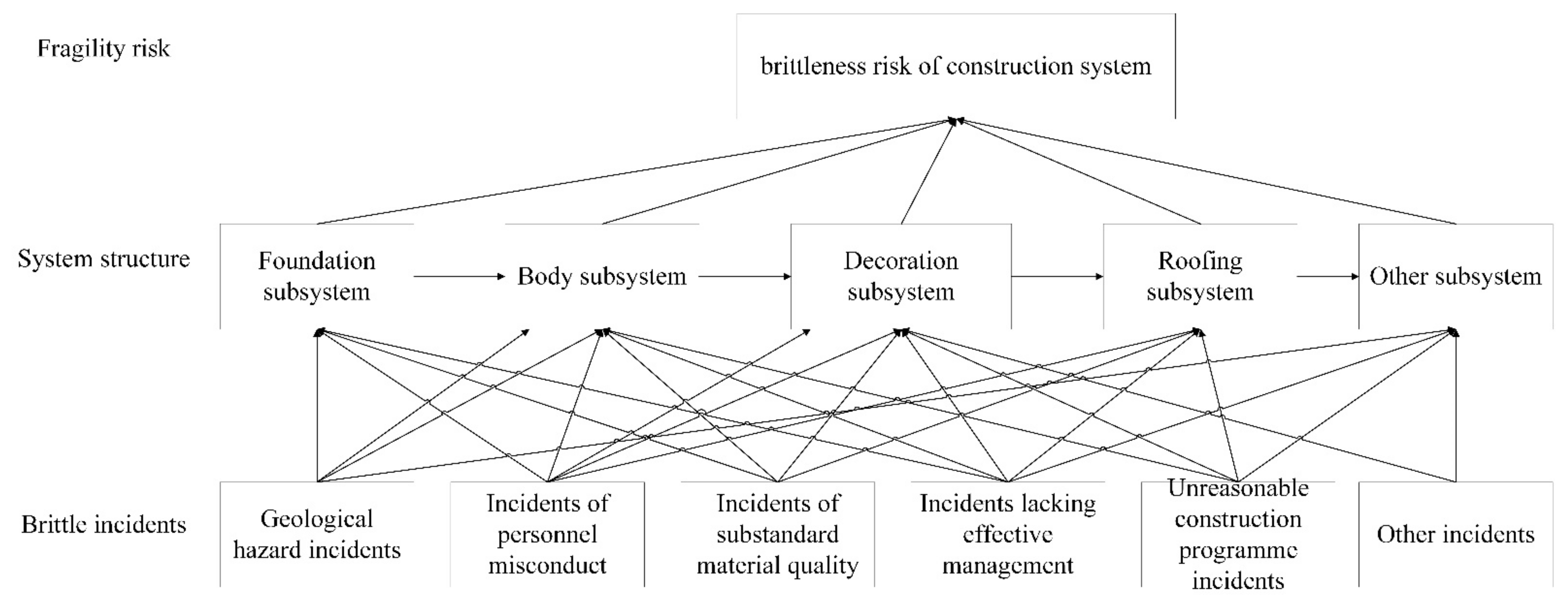
We often divide the process of constructing a complete building into sub-projects such as foundation construction, main body construction, decoration construction, and roof construction. By applying the theory of complex system fragility to the construction process and combining it with the traditional Work Breakdown Structure (WBS) in project management, a theoretical system of risk in the construction process from the perspective of fragility can be obtained (
Figure 3). The brittle structure model examines the brittle characteristics of risk hazard complex systems from the perspective of coupled inner and outer factors. In fact, this model is used to address the loss of the original state of the system during construction.
5. Buffer Sizing Method Based on Brittle Risk Entropy
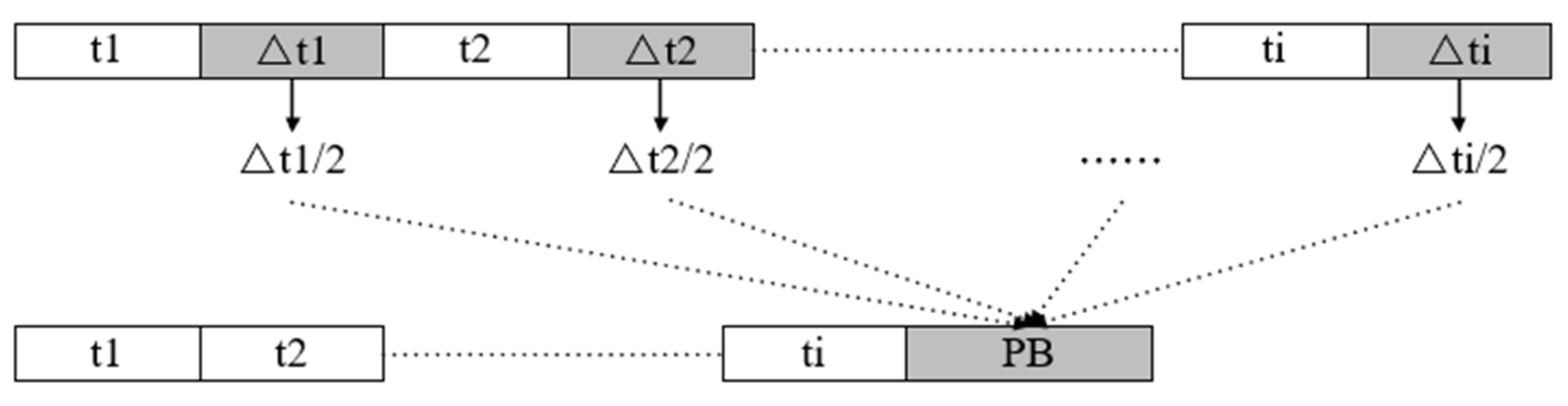
We now describe the uncertainty of the internal risk of complex systems with the help of brittle risk entropy, based on the Root Square Error Method. The Root Square Error Method is based on the central limit theorem [
20]. Its proposition is to determine the safe time of the process by calculating the variance and to calculate the buffer size by twice the standard deviation of the link. This fully satisfies the rules of fuzzy time accumulation. The principle is shown in the
Figure 4. The specific calculation formula is as follows.
where,
is used to indicate the safety time of individual tasks on or off the critical chain.
We have divided the buffer settings into two parts, one for the project buffer and the other for the feeding buffer.
The project buffer size is calculated from Equation (11).
where
is the project buffer,
is the set of processes in the critical chain,
is the critical chain system brittleness risk entropy and
is the safety time of activity i.
The feeding buffer size is calculated by Equation (12).
where
is the feeding buffer of the
Kth non-critical chain,
is the set of processes on the
Kth non-critical chain,
is the system brittleness risk entropy of the
Kth non-critical chain, and
is the safety time of activity
j.
The feeding buffer size derived according to Equation (12) may be large, causing resource conflicts when the buffered non-critical chains sink into the critical chains. Therefore, we needed to make corrections to the size of the project buffer. The correction was made by passing the free time differences of the processes at the end of the non-critical chain through the feeding buffer, while the remaining values of the buffers in each non-critical chain were incorporated into the project buffer. The specific steps are as follows.
Step 1. We can compare the magnitude of the free time difference between the end process on a non-critical chain and the value of the feeding buffer, and take the smaller as the correction value for the feeding buffer on this chain. The relevant formula is as follows.
where
is the free time difference of the last process
P on the Lth non-critical chain,
is the lesser of
and
to avoid resource conflicts causing changes to the critical chain,
is the earliest start time of process
j and
is the earliest end time of process
P.
Step 2. The remaining buffer value for the Lth non-critical chain can be calculated from Equation (15).
where
is the feeding buffer of the Lth non-critical chain.
Step 3. As a result, we can derive a revised value for the project buffer in the critical chain.
where
is the sum of the remaining buffer values.
6. Application
Now we illustrate the process based on the brittle risk entropy model described in the previous section with a case study.
6.1. Information of the Project
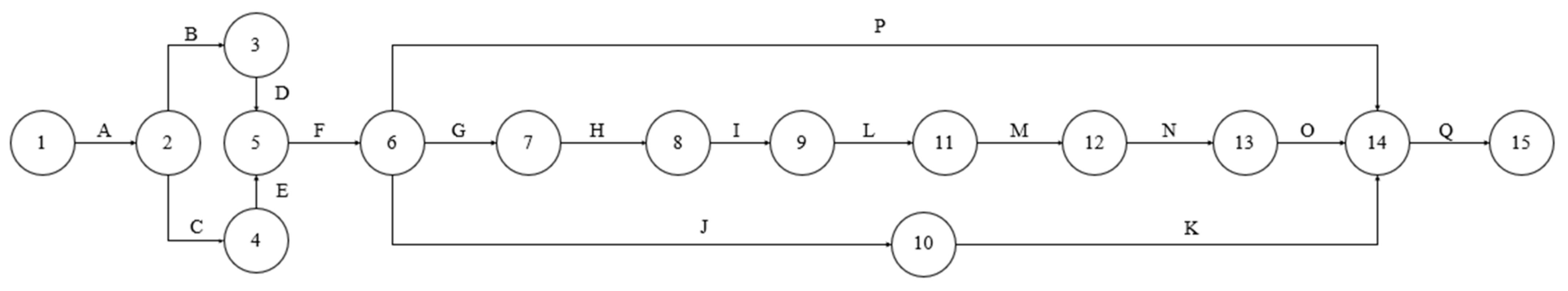
The project consisted of 17 activities, each requiring 3 resources (r1, r2, r3) and a resource limit of (6, 8, 5). Specific information about each activity in the project is shown in
Table 1. The network plan diagram is shown in
Figure 5.
The activity times
were estimated using a trapezoidal whitening power function [
46], while the safety time
was estimated using fuzzy theory [
47]. Information on the activity time is shown in
Table 2, where
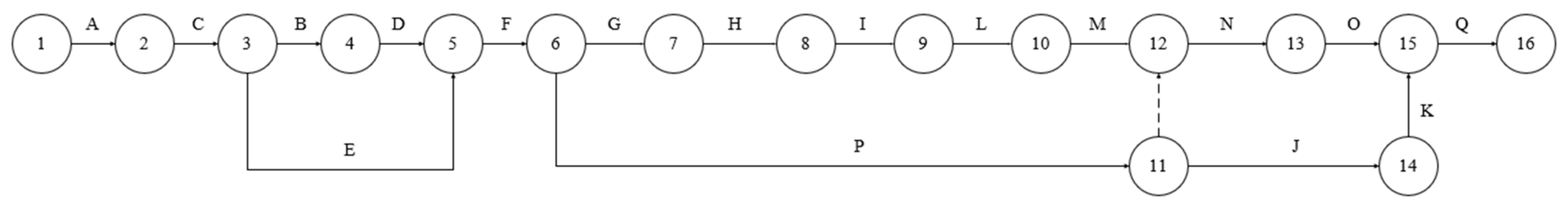
indicates the consistent duration value for process i at a 95% completion rate. As the project was executed due to the existence of resource conflicts, an adjusted network plan diagram (
Figure 6) for the project can be obtained using a heuristic algorithm based on a critical chain identification model with multiple resource constraints. The adjusted network plan diagram shows that the critical chain is A–C–B–D–F–G–H–I–L–M–N–O–Q, with a desired total duration of 28.17 days.
6.2. Application of the Brittleness Risk Entropy Function
The range of probability distributions expected for the outcome of various risks can be obtained by experts in conjunction with historical statistics. Firstly, we used a random number generator to generate random numbers to simulate the likelihood of a risk occurring. Secondly, we determined the impact of the risk with the help of the probability distribution range. Finally, the risk weights were combined to calculate the combined impact rate of the risks. The following was used as an example to calculate the combined impact rate of risk for activity A.
The probability distribution of activity A (
Table 3) can be obtained from the historical data and expert opinion. We used a random number generator to generate a set of random numbers as
, and then we compared the random numbers with
Table 3, from which we could obtain the effect of risk as
. Similar to the previous, we chose 1000 groups for the randomized trial, which yielded many group randomization numbers and risk impact effects.
In order to assign weights to the impact of risk events on Activity A, four experts were invited to rank the importance of the most likely risk incidents B1 to B5 in Activity A respectively. Using Equations (7)~(10), a matrix of relative risk weights for Activity A can be obtained.
We can use Equation (6) to find the combined impact rate C for a combination of 1000 random numbers, taking the median of which is the actual risk combined impact rate for activity A. Similarly, the combined impact rate of risk for other activities can be found (
Table 4).
We used the Delphi method to identify the extent,
, to which a subsystem crash affects a system crash. Eight experts were invited. Firstly, we obtained initial comments from the experts. Then, we collated, summarized and tallied the data. After that, anonymous feedback was given to the experts for a second opinion. Finally, the extent of impact
was determined (
Table 4).
6.3. Calculation of Buffer Size
The critical chain activities included A, C, B, D, F, G, H, I, L, M, N, O and Q. The project buffer value was calculated as 7.845 d according to Equation (11). The non-critical chain activities included E, P, J and K. The feeding buffer was calculated according to Equation (12), which gave a feeding buffer of 1.644 d for the non-critical chain E, 2.157 d for the non-critical chain P and 3.388 d for the non-critical chain P–J–K.
We tried to avoid problems such as resource conflicts and aborts during critical chains. Based on Equations (13)~(16), the remaining buffering of possible non-critical chains was calculated and considered for correction. In this case, the feeding buffers were all less than the free time difference, their remaining buffers were all zero and there was no remaining buffer for non-critical chains.
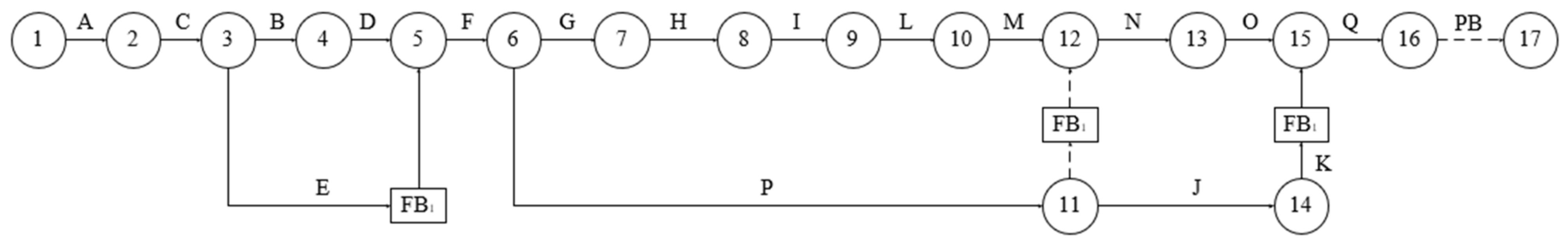
The project buffer values
calculated above were set at the end of the critical chain. The feeding buffer values
,
,
from the above calculation were set at the end of the non-critical chains E, P, and P–J–K respectively. The specific location of the setting is shown in
Figure 7. The adjusted network plan diagram gives a desired total duration of 36 d.
6.4. Comparative Analysis
In order to reflect the adaptability and superiority of our method, the Cut-and-Paste Method (C&PM), the Root Square Error Method (RSEM), and the buffer calculation method proposed by Gong Jun et al. [
25] were selected for comparison and analysis with the setup method in this paper. This comparison was carried out using 1000 Monte Carlo simulations with Crystal Ball software, set at a 95% confidence level [
48]. The durations of all methods satisfy the triangular distribution. The buffer sizes obtained by each method are shown in
Table 5. The probability of completion for the different methods is shown in
Table 6.
As can be seen from
Table 5, the method used in the paper calculates a shorter planned project completion period than the Cut-and-Paste Method (C&PM) and the method proposed by Gong Jun et al. [
25] but is longer than the Root Square Error Method (RSEM). We believe that the reasons for this situation are as follows.
- (1)
The Cut-and-Paste Method can lead to excessive buffer settings as the links get longer [
49]. This case consisted of 17 activities, which make up a long chain. We used the Cut-and-Paste method to calculate buffers, which can lead to too large a buffer that eventually lasts too long.
- (2)
The Root Square Error Method failed to measure project-specific uncertainties [
50], resulting in the setting of a small buffer that ultimately led to the original plan to deviating from reality.
- (3)
Although the buffer size calculation method proposed by Gong Jun et al. [
25] takes into account the uncertainty in the construction process and divides it into multiple objectives for quantification, it does not consider the correlation between the various set objective factors.
- (4)
The total duration of project completion under different completion probabilities obtained using this method is better than the other two methods, except for the root variance method. During actual construction, if the buffer size was managed appropriately, the real completion time will be smaller than the simulation prediction. Therefore, it is effective and reasonable to use the improved critical chain approach to project construction schedule management from a systems perspective.
7. Conclusions
From the available literature, the setting of CCPM buffers has mostly been studied having been divided into different attributes [
51]. However, this situation does not take into account the correlation between attributes, which can lead to the emergence of new uncertainties. This study proposes a new method for resizing buffers from a system perspective. The method draws on the concept of entropy to measure uncertainty in the progress process. In addition, a brittle risk entropy function has been constructed with the help of the combined risk impact rate, as a way of avoiding the singularity of starting from an attribute. Finally, this paper took a project as an example and compared the effectiveness of the method proposed in this paper, the method proposed by Gong Jun, C&PM and RSEM, and we conclude that the method has a certain degree of effectiveness and feasibility.
This study contributes to CCPM research in the following ways:
- (1)
Brittle risk entropy can be used to describe the uncertainty of potential risks within a complex system. There is a great deal of uncertainty in the progress process, which needs to be quantified and described. We were the first to introduce the concept of brittle risk entropy into the determination of project buffers.
- (2)
The emergence of new methods has led to new directions for the subsequent development of the theory. The approach to critical chain buffer setting from a system perspective is complemented by our study based on brittle risk entropy.
Because of the huge economic value involved, buffer size settings are critical to CCPM. There should be a direct economic value to the project management company for the work we do, mainly for the following reasons. First of all, the approach we propose is applicable to most projects, especially large and complex ones. Secondly, the conclusions we drew from applying the method to the case in our paper are clearly justified and provide a more accurate and robust estimate of the project’s duration. In the actual project management process, we need to consider both the economic interests of the owner side and the reasonable construction time of the project builder, and the method proposed in this paper can help project companies to avoid the problems of underestimation and overestimation.
We have been too constrained in our study of buffer settings, and in fact the issue can be approached from a number of angles. It is interesting to set up the buffer with the help of entropy theory. In addition, we can also draw on other concepts that can describe uncertainty, such as probabilistic rough sets, cloud models, fuzzy sets, etc., [
52]. Undoubtedly, the study of buffers from a systems perspective needs more attention and this will be one of the key directions for future research on buffer settings. Further, we will focus on how the calculation of brittle risk entropy can be fully quantified, which is both a shortcoming of this paper and the focus of our future research.


