Comparison Study of the Heating Energy Demand for a Multi-Storey Residential Building in Romania Using Steady-State and Dynamic Methods

Abstract

The purpose of this study is to determine the differences between the steady-state energetic method and the dynamic energetic method in a multi-storey residential building in Romania. For both methods, there are two values for the heating energy demand, one obtained with the theoretical U value and g value according to Romanian Methodology Mc 001/1-2006 and one with the real U value and g value obtained from in situ measurements. The results of our study revealed a difference between the steady-state method and the dynamic method in both cases of approximately 20%. Because the heating energy demand needs to decrease in value according to European legislation and the classical energy demand determination is shallow, as it does not take into account some important factors, it is important to use a method that produces accurate values so the economic factor does not become overwhelming.

1. Introduction

At the European level, the goal for the future has transformed into an obligation that was laid down in the first European Climate Law. The EU target is to become the first climate-neutral continent by 2050. To achieve this goal, the first step is to reduce greenhouse gas emissions by at least 55% by 2030 (compared to 1990). The revision of the Energy Performance of Buildings Directive, planned for later in the year, will identify specific measures to accelerate the rate of building renovations, contributing to energy efficiency and renewable goals, as well as greenhouse gas emissions reductions, in the building sector.

To meet the 2050 energy targets, the renovation rate of the building stock must increase. The building sector is responsible for about 40% of global energy use, of which space heating and cooling consume approximately 60% [1]. Buildings are also responsible for a large share of CO₂ emissions in the EU, accounting for about 36%. For these reasons, the building sector represents a large potential for significantly reducing energy demand and the harmful emissions [2].

A possible solution involves retrofitting existing buildings to net-zero energy buildings by enhancing the envelope efficiency, resulting in reduction in energy usage of the building while also integrating renewable energy with the existing structure to generate clean energy [2].

The envelope plays the most important role in the energy consumption of a building. Numerous strategies can be adopted to design building facades for nearly zero-energy buildings. Some authors [3,4,5,6,7,8,9,10] have studied ways to optimize the envelope of buildings to achieve the nearly zero-energy goal in various climate zones.

A study realised by F. Ascione showed that it is difficult to achieve nZEBs in the Mediterranean climate, taking into account a high standard of thermal comfort [3]. A study realised in a hot climate [4] showed that a nZEBs would be an economic benefit for the population, and in the future, with new technologies on the way, it would be much easier and cheaper to realise nearly zero-energy buildings. Buonomano [5] studied the energy efficiency of non-residential buildings using a computer model that can predict the energy demand of buildings integrating new technologies. A study conducted in Norway [6] on Greek residential buildings showed that for every climate zone in Greece, there a different combination of measures is ideal with respect to achieving a nearly zero-energy buildings. Loukaidou conducted a study in Cyprus [7], which included a cost-optimal analysis of thermal features of the building envelope. C. Micono [8] designed a building that, according to the analyses, is able to produce the same amount of energy as it consumes on a yearly basis. A study realised in Ireland [9] that compared a super-insulated building to a building that uses renewable technology showed that the super-insulated building is more cost-efficient due to the fact that the cost of electricity, gas and wood pellets is expected to increase in the future. K. Zakis performed an analysis of 11 buildings [10] with the aim of increased energy efficiency using a dynamic simulation.

The first step in the renovation of a building is to determine the relevant energetic details. In this study, we considered the U value and g value of the envelope.

The U value can be determined using a non-destructive method, such as a quantitative IR thermography method or a heat flow meter. The IFT method offers quick results but depends on solar radiation, which can affect the results, whereas the HFM method requires a longer period to obtain results and depends on the temperature difference between the exterior and interior, the wind speed and temperature fluctuations, as shown by Rosano Albatici et al. and I Nardi et al. in two separate studies [11,12]. In the current study, the HFM method is used, and the measurement is valid for 15 days due to unsteady conditions.

The U value can be determined calculated according to the normative layers of elements in the building. The layers can be provided in the project design of the building or determined using a destructive method that involves sampling with a hollow drill. If there are stable conditions, then the non-destructive method is the preferred choice, according to Giuseppe Desogus [13].

According to some studies [11,12,14,15] there is a worldwide discrepancy between theoretical U values and the real U values obtained from various in situ measurements. Studies have been conducted on both old buildings and new buildings. The real U value obtained using a heat flux meter is often higher than the theoretical U value determined using national codes [11,12,15,16]. The results depend on climatic parameters, such as solar radiation, wind speed, the difference between the interior and exterior temperature and elemental orientation.

Several conditions must be satisfied to achieve precise measurements. The values obtained from in situ measurements may be incorrect if these conditions are not met. Factors that can contribute to inaccurate measurements include incorrect placement of the heat flux sensor on the analysed envelope element; moisture inside the element (especially for walls), leading to increased conductivity; weather conditions; and interior temperature variations. Measurement conditions must be stable [17].

According to a study conducted in South Korea [18], the attachment method of the heat flux sensor has a particular importance with respect to the results. Tests were conducted in a test room and a heating room, in addition to in situ tests in existing buildings. Three attachment methods we applied: using a tape, thermal conductive paste and a thermal pad. The authors concluded was that using a tape, there is a possibility of an air gap between the tape and the element, which could perturb the results. With the use of thermal conductive paste, the adhesive surface may not be clean, as it has to be applied by hand, which could impact the results. In contrast, with the use of a thermal, there is a low probability of inaccurate results.

Another conclusion of the authors of the above-mentioned study [18] is that if the temperature difference between the interior and exterior is small or the existing insulation is excellent, then the heat flux transfer is irrelevant, which could lead to imprecise results.

For the measurements to be accurate, there must be a difference between the interior and exterior temperatures [19]. A smaller temperature difference results in a higher U value, with increased uncertainty [13]. A higher temperature difference (19 °C) requires a test duration of a minimum of 72 h [20], whereas a smaller difference (<13 °C) would prolong the test [21].

The temperature difference between the interior environment and the exterior environment should be higher than 15 °C; however, if these conditions cannot be satisfied, a temperature difference of at least 5 °C is acceptable [17]. Because the sensor measures conductivity, convection and radiation, it is necessary to avoid the solar radiation. This can be achieved by conducting measurements on a facade oriented to the north or conducting measurements at night. The ideal measurement conditions include an absence of precipitation and wind speeds not exceeding 1 m/s, as wind increases the heat transfer speed.

Measurement of the U value may depend on the orientation of the building; a study showed that the thermal transmittance value measured on an east-facing wall is higher than that measured on a north-facing wall [22].

Temperature variations could have a negative effect on the results, which is why it is preferable that the exterior temperature not change by more than 5 °C and that the interior temperature does not vary by more than 2 °C [17].

According to a study conducted by Bienvenido-Huertas et al. at the University of Sevilla, measurements conducted in the winter are more accurate than those conducted in the summer, due to considerable temperature differences between the interior environment and the exterior environment [17].

Another important factor with respect to obtaining precise measurement is the position where sensors are mounted. The location may be chosen after conducting a thermographic analysis on the envelope (according to ISO 10878:2013) [23]. The heat flux sensor should be in direct contact with the element. The surface also must be smooth, with no moisture or dust. Before mounting the sensor, the surface is cleaned with ethanol. A thermal pad is used to mount the sensor in order to ensure that there is no air gap between the sensor and the thermal pad or between the thermal pad and the wall surface.

The orientation of the sensor is crucial. The thermal flux is oriented from the hot zone to the cold zone. The heat flux sensor should be mounted with the positive side of the sensor in the direction of the positive heat flux. However, the heat flux sensor could be mounted in both directions: if the direction of the heat flux changes, the voltage value sign changes (from positive to negative and vice versa).

The purpose of the current study is to highlight the difference between values outlined in the standards and actual values obtained by in situ measurements. By determining the real characteristics of the building envelope, it is possible to propose the most suitable type of renovation for a building. With this research, we also aim to verify the accuracy of the steady-state method by comparing it with the dynamic method. A verified dynamic model under initial design boundary conditions can be used to more accurately observe energy performance indicators [24]. Such a model can be then used to propose solutions for the planning phase with respect to interventions in existing buildings to achieve improved energy efficiency [25].

2. Materials and Methods

2.1. Methodological Approach

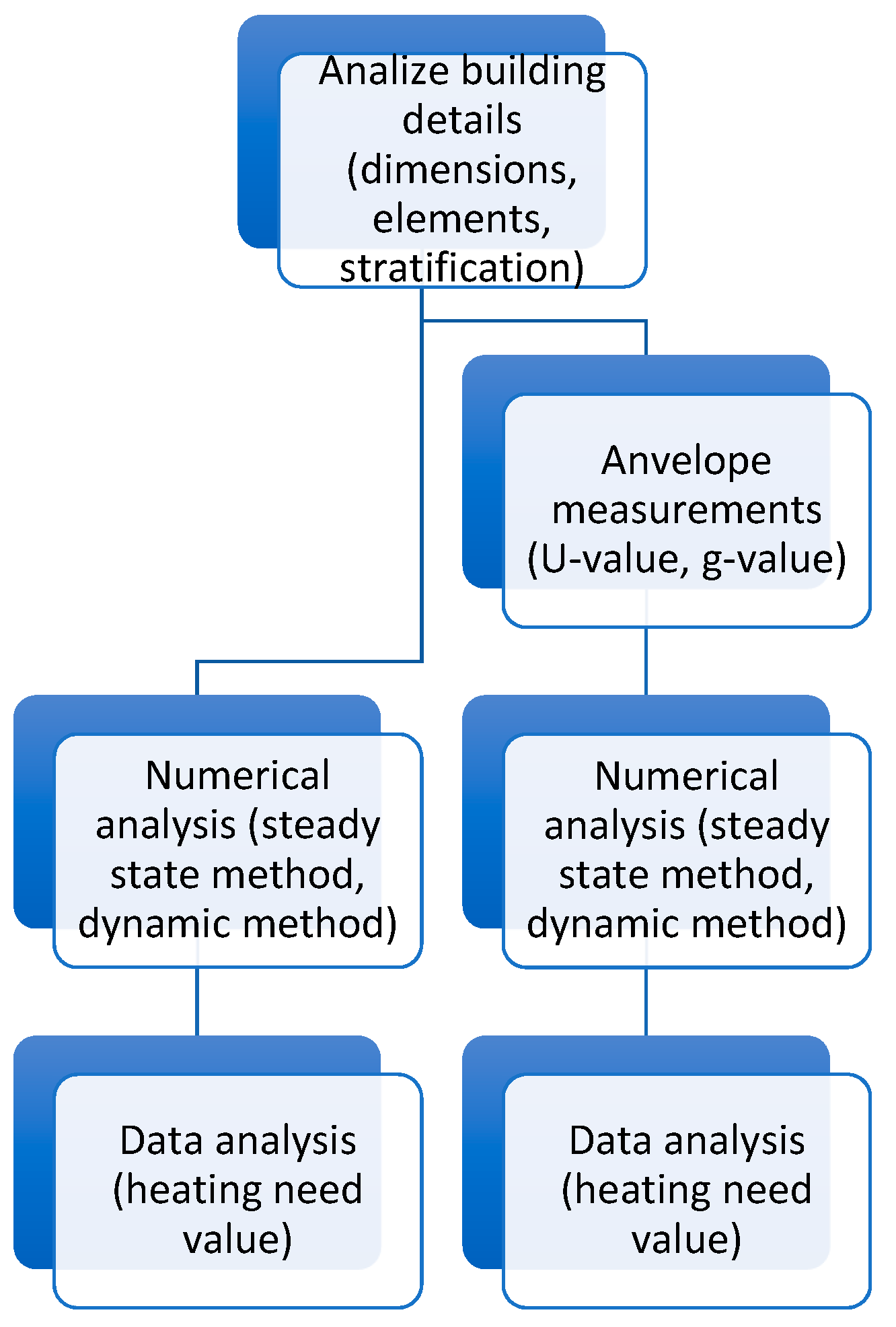
Heating energy demand can be determined in two ways. The first involves the use of the steady-state method, and the second one involves the use of the dynamic method. For both methods, there two determinations must be made; the first involves the theoretical U value and g value, whereas the other method requires the real U value and g value obtained from in situ measurements. U values are obtained by measuring the heat flux through an exterior element using a heat flux sensor, and the g value is obtained by measuring the transmission of energy through glazed elements.

The purpose of the article is to highlight the necessity of adapting the steady-state method according to variable parameters: internal gains, the number of air changes, the U value, the g value and solar gains.

With respect to internal gains, in this study, we took two types of internal gain into account: those generated by people who live in the building and the those generated by lightning equipment. Under the steady-state method, internal gains are constant, whereas when using the dynamic method, the two values vary, providing a more accurate determination of the heating requirements. The steady-state method assumes that the building is at full capacity at all times and that the lightning equipment is used 24 h per day, which is not true.

The number of air changes in the case of the steady-state method is adopted from a table depending on the location of the building.

The U value is used in conformity with national regulations, which results in the value being over-rated. The real U value can be determined by in situ measurement. One method of obtaining the U value is to measure the heat flux that passes through the element. The real g value can be determined by in situ measurement of the transmission of energy through glazed elements. Measurements can be taken immediately, with no strict conditions to be fulfilled. The value is affected by the age of the element, with higher values associated with older elements.

Solar gains are considered, although in a simplified way, when using the steady-state method. Solar gains play a significant role in the dynamic method, with solar heat taken into consideration for every day of the year.

We concluded our study by comparing the four values of heating demand obtained by using the two data analysis methods and two types of thermal values, i.e., a theoretical value and a measured value, as shown in Figure 1.

2.2. Object of Study

In the current study, we analysed a building located in Timișoara, Romania. The building is a residential building constructed before 1989. We conducted measurements on the building, which is a typical T770-IPCT typology Pb4 building in the city of Timisoara. The building is occupied, so a permit was required to take the measurements. The structure is composed of precast elements, a common building material for that period. The building has five floors and basement. Each floor has four apartments.

The building envelope is detailed in

Table 1. Stratification of the elements that form the building envelope.

	Description		Area [m²]	Layers (Interior to Exterior)
				Material	Thickness (m)
Exterior walls	N	Precast concrete walls	29.4	Reinforced concrete	0.125
	S		29.4	AAC	0.085
	V		233.45	Reinforced concrete	0.06
	E		234.28	Cement mortar	0.01
Interior walls	N	Precast concrete walls	137.2	Reinforced concrete	0.125
	S		0	AAC	0.085
	V		0	Reinforced concrete	0.06
	E		0	Cement mortar	0.01
Ground floor slab	-	Reinforced concrete slab	305.9	Parquet	0.02
				Reinforced concrete	0.13
Top floor slab	-	Reinforced concrete slab	305.9	Reinforced concrete	0.13
				AAC	0.1
				Concrete	0.04
Exterior windows	N	Wooden windows with two glass layers	0	Woodwork with two glass layers with a distance of 2–4 between layers	-
	S		0
	V		87.75
	E		86.91
Exterior doors	N	Metal doors	0	Aluminium door with insulating glass	-
	S		0
	V		3.47
	E		1.68

. The data on the building envelope were obtained from the institute that designed it. The table shows the surface of each element, calculated for every orientation, as well as the layer of the element and its thickness, listed from the interior surface to the exterior surface.

The north and south walls are considered interior elements because of the attached neighbouring buildings. These walls are not exposed to wind or solar radiation, although heat loss does occur through this element.

2.3. Equipment

2.3.1. Equipment Used for Measuring the U Value

• Principles

The U value is calculated based on the measurement of the heat flux that crosses an element determined by a heat flux sensor and the temperature on both sides of the element under steady conditions. Because stable conditions are difficult to achieve for in situ measurements, measurements must be conducted over a longer period of time, with the value calculated as the average of the stabilized values during the measurement period.

The method is described in ISO 9869-1:2014 [21].

2.

Conditions and criteria for accurate measurements

To realise a precise measurement, some climatic conditions must be satisfied. In this case, the measured wall is located on the northwest side of the building. Considering the context, solar radiation has a considerable impact on the analysed element in the afternoon. Therefore, the period of time when the sun hits the element is not taken into account because the exterior thermometer is heated up and does not display the correct temperature. The wind speed was moderate at the time of measurement, so it did not affect the obtained value. The interior temperature was constant, as the apartment has a thermostat that keeps the temperature steady. The interior-to-exterior temperature difference was measured at night, so only those periods of time were taken into consideration. The measurement took place over a 15-day period, in accordance with the required 72 h minimum measurement time and the calibration period of the device.

3.

Equipment

The equipment used for this measurement was developed by greenTEG, Zurich, Switzerland. It is composed of a gSKIN DLOG data logger, two temperature sensors and a gSKIN heat flux sensor, which measures the thermal power.

The thermal sensor comprises five layers: the package, contacts, thermopiles, substrate and interconnects. The thermopiles are electrical devices that convert the thermal energy into electric energy and are made of thermocouples. The device generates voltage when the thermocouples are exposed to temperature variations. The thermopiles are integrated into the sensor substrate, which leads to a high sensitivity of the sensor.

2.3.2. Equipment Used to Measure the g Value

• Principles

Total transmittance of solar energy, or the g factor, is the sum of direct solar transmittance (τe) and the secondary inward heat transfer factor (qi); the latter results from the transfer of heat by convection and long-wave IR radiation from the portion of incident solar radiation that was absorbed by the glazing.

The method is described in ISO 9050:2003 [26].

The adopted method is very fast and accurate, with actual measurement achieved in real time (just 5 s).

2.

Conditions and criteria for accurate measurements

In order to achieve precise measurements, the investigated elements must be clean and kept in a fixed position during the measurements. Indoor and outdoor temperature variations, sun radiation and wind speed do not affect the measurement.

3.

Equipment

The equipment used for this measurement is called an SS2450solar spectrum transmission meter (manufactured by Electronic Design to Market, Inc., Toledo, OH, USA). This device is used to measure the transmission of energy through glazed elements. Compared to other devices on the market, it has the ability to produce and measure almost the entire solar spectrum. It has 12 light sources on one side with wavelengths ranging from 300 to 1700+ nm, 3 light sensors on the opposite that measure the rays that reach them.

2.4. Measurement Procedure for the U Value

2.4.1. Equipment Mounting

First, the mounting position must be chosen for the sensors. This is a very important step with respect to obtaining accurate results. The heat flux sensor should be in direct contact with the element. The surface should be smooth and cleaned with ethanol. A thermal pad (30 × 30 × 5 mm) is used to mount the sensor to ensure that there is no air gap between the sensor and the thermal pad or between the thermal pad and the wall surface. The thermal flux is oriented from the hot zone to the cold zone. In this study, the positive side of the sensor was oriented toward the interior environment.

To obtain the U value, the interior and exterior temperatures must be measured. (Figure 2).

The data provided by the heat flux sensor and the two temperature sensors are recorded in fixed intervals of 10 min. The interval duration and the minimum test duration depend on the nature of the element, the interior and exterior temperature and the method being applied. The minimum test duration is 72 h if the temperature is stable.

Measurements to determine the U value of the walls were performed for a period of 15 days, but only the measurements values obtained in the last 7 nights of this period were considered. Due to solar radiation, the results obtained on the other days were erroneous. Because the elements are situated on the northwest side and solar radiation was very strong during the daytime, the exterior temperature sensor was overheated, resulting in higher temperatures than the actual values, even at night. In the last 7 days of the measurement period, during daytime, there were rain showers, so the level of solar radiation was low and did not affect the temperature sensor. Because the equipment used to measuring the g value is a device that performs instantaneous measurement, there was no need for the device to be mounted on the window a long period. After the device was switched on, a couple of seconds were required for self-calibration. When the calibration was completed, the device displayed a value 100 on the g-value screen, indicating that measurements could be started. The device has to be kept in a perpendicular position on the glass during the entire measurement.

Three measurements were conducted to ensure accuracy. The g value was determined on the same window on which the U value was determined.

2.4.2. Data Collection

After the equipment was mounted, the measurement was set to start immediately, collecting data every 10 min. The measurements were performed for 15 days, taking into account only the results obtained at night. Only the data obtained over the last 7 nights of the measurement period were considered. The heat flux sensor required calibration period, so the first days of measurements were not taken into account (Figure 3).

The U value was obtained by dividing the heat flux density by the temperature difference and averaging the obtained values.

$$U=\frac{{{\displaystyle \sum }}^{}q}{{{\displaystyle \sum }}^{}\left(T_i-T_e\right)}$$

(1)

where:

q—heat flux density, W/m²;

T_i—interior temperature, °C or K; and

T_e—exterior temperature, °C or K.

In order for the results to accurately reflect reality, the following three conditions must be respected:

• Condition 1. The duration of the test in which the temperature is stable must be at least 72 h; otherwise, the duration may be extended. For buildings with a high thermal capacity, the duration is extended (not less than 96 h).
• Condition 2. The v thermal resistance value (R) obtained at the end of the test should not vary by more than +/−5% from the value obtained 24 h earlier. The following formula is used to obtaining the thermal resistance value:

  $$R=\frac{1}{U}-R_{si}-R_{se} [\frac{{\mathrm{m}}^2\mathrm{K}}{\mathrm{W}}]$$

  (2)

  where:

R—total thermal resistance;

U—thermal unidirectional transmittance; and

R_s—superficial thermal resistance (interior/exterior).

• Condition 3. The thermal resistance value (R) obtained during the first time interval (INT (2 × D_T/3) days) should not vary by more than +/−5% from the value obtained during the last time period of the same duration. D_T is the duration of the test measured in days, and INT number of days rounded to the nearest whole.

  $$\mathrm{INT}\left(\frac{2\times \mathrm{DT}}{3}\right)=\mathrm{INT}\left(\frac{2\times 7}{3}\right)=\mathrm{INT}\left(4.66\right)=4$$

  (3)

In this case, the thermal resistance value obtained at the end of the first four days did not vary by more than +/−5% with respect to the value obtained at the end of the last four days.

2.4.3. Wall Measurements

The final U value was calculated by averaging the seven obtained values (

Table 2. Average nigh value of the thermal transmittance for the exterior wall.

	U (W/m²K)	Percentage Difference from the Average Value (+/− %)
Night 1	1.279	−2.9%
Night 2	1.327	0.9%
Night 3	1.303	−0.9%
Night 4	1.353	2.8%
Night 5	1.318	0.2%
Night 6	1.342	2.0%
Night 7	1.313	−0.2%
Average	1.316

U—average value of the thermal transmittance obtained from one night of measurements.

).

• Condition 1. The duration of the U-value test was 75 h, surpassing the minimum duration.
• Condition 2. The thermal resistance obtained after in situ measurements was:

  $$R_{\mathrm{final}}=\frac{1}{1.316}-0.125-0.042=0.593 [\frac{{\mathrm{m}}^2\mathrm{K}}{\mathrm{W}}]$$

  (4)

The thermal resistance obtained 24 h before finalizing the measurements was:

$$R_{24\mathrm{h}\mathrm{before}}=\frac{1}{1.313}-0.125-0.042=0.594 [\frac{{\mathrm{m}}^2\mathrm{K}}{\mathrm{W}}]$$

(5)

The percentage difference between the two values was 0.17%, meaning that the condition was satisfied.

• Condition 3. The thermal resistance value obtained at the end of the first four days was:

  $$R_{\mathrm{endfirst}4\mathrm{days}}=\frac{1}{1.353}-0.125-0.042=0.572 [\frac{{\mathrm{m}}^2\mathrm{K}}{\mathrm{W}}]$$

  (6)

The thermal resistance value obtained at the end of the last four days was:

$$R_{\mathrm{endlast}4\mathrm{days}}=\frac{1}{1.313}-0.125-0.042=0.594 [\frac{{\mathrm{m}}^2\mathrm{K}}{\mathrm{W}}]$$

(7)

The percentage difference between the two values was 3.70%, meaning that the condition was satisfied.

The specified conditions must be satisfied to validate the results.

2.4.4. Window Measurements

The final U value was calculated by averaging the seven obtained values (

Table 3. Average nigh value of the thermal transmittance for the windows.

	U (W/m²K)	Percentage Difference from the Average Value (+/− %)
Night 1	2.91	0.3%
Night 2	2.92	0.7%
Night 3	2.88	−0.7%
Night 4	2.89	−0.3%
Night 5	2.90	0.0%
Night 6	2.93	1.0%
Night 7	2.88	−0.7%
Average	2.90

).

• Condition 1. The duration of the U-value test was 75 h, surpassing the minimum duration.
• Condition 2. The thermal resistance obtained after in situ measurements was:

  $$R_{\mathrm{final}}=\frac{1}{2.90}=0.344 [\frac{{\mathrm{m}}^2\mathrm{K}}{\mathrm{W}}]$$

  (8)

The thermal resistance obtained 24 h before finalizing the measurements was:

$$R_{24\mathrm{h}\mathrm{before}}=\frac{1}{2.88}=0.347 [\frac{{\mathrm{m}}^2\mathrm{K}}{\mathrm{W}}]$$

(9)

The percentage difference between the two values was 0.86%, meaning that the condition was satisfied.

• Condition 3. The thermal resistance value obtained at the end of the first four days was:

  $$R_{\mathrm{endfirst}4\mathrm{days}}=\frac{1}{2.89}=0.346 [\frac{{\mathrm{m}}^2\mathrm{K}}{\mathrm{W}}]$$

  (10)

The thermal resistance value obtained at the end of the last four days was:

$$R_{\mathrm{endlast}4\mathrm{days}}=\frac{1}{2.88}=0.347 [\frac{{\mathrm{m}}^2\mathrm{K}}{\mathrm{W}}]$$

(11)

The percentage difference between the two values was 0.29%, meaning that the condition was satisfied.

The specified conditions must be satisfied to validate the results.

2.5. Measurements Procedure for the g Value

After the device was calibrated and mounted on the glass, the measurements were started. To ensure an accurate measurement, we conducted three readings on the same window, with the requirement that all three measurements return the same value. The device displays a value of 100 to confirm the accuracy of a measurement.

2.6. Comparison with Theoretical Values

The measured U value was further compared with the theoretically determined value to determine the difference. According to Romanian Methodology Mc001/1-2006, the U value for an element was obtained using the following equation:

$$U=\frac{1}{R}\left[\frac{\mathrm{W}}{{\mathrm{m}}^2\mathrm{K}}\right]$$

(12)

The value of the thermal resistance was obtained using the following relation:

$$R=R_{si}+{{\displaystyle \sum }}^{}{R}_j+{{\displaystyle \sum }}^{}{R}_a+R_{se} [\frac{{\mathrm{m}}^2\mathrm{K}}{\mathrm{W}}]$$

(13)

where:

R_j—transmission thermal resistance of a homogeneous layer (j); and

R_a—thermal resistance of an air layer.

$$R=0.125+0.37+0.042=0.537 [\frac{{\mathrm{m}}^2\mathrm{K}}{\mathrm{W}}]$$

(14)

We took into account the reduction coefficient of the thermal conductivity due to material aging and the presence of dampness.

The U value obtained for the wall from the in situ measurements was 1.316 $\left[\frac{\mathrm{W}}{{\mathrm{m}}^2\mathrm{K}}\right]$, whereas the theoretically determined U value was 1.86 $\left[\frac{\mathrm{W}}{{\mathrm{m}}^2\mathrm{K}}\right]$ (

Table 4. Calculated value of the thermal transmittance.

Material	d (m)	λ (W/mK)	a (–)	λ’ (W/mK)	Rj (m²K/W)	R (m²K/W)	U (W/m²K)
Reinforced concrete	0.125	2.03	1.1	2.23	0.06	0.537	1.86
AAC	0.085	0.24	1.3	0.31	0.27
Reinforced concrete	0.06	2.03	1.1	2.23	0.03
Mortar cement	0.01	0.93	1.3	1.21	0.01
Total:					0.37

d—layer thickness (m), λ—thermal conductivity (W/mK), a—reduction coefficient (–), λ’—corrected value of the thermal conductivity (W/mK).

). The percentage difference between the two values was 29.24%, which is a significant difference. This difference corresponds to the analysed building on one orientation and during a single period of the year.

The U value obtained for the window from the in situ measurements was 2.90 $\left[\frac{\mathrm{W}}{{\mathrm{m}}^2\mathrm{K}}\right]$, whereas the theoretically determined U value was 3.03 $\left[\frac{\mathrm{W}}{{\mathrm{m}}^2\mathrm{K}}\right]$. The percentage difference between the two values was 4.29%, which is a less significant difference that that obtained for the wall.

The g value obtained for the window from the in situ measurements was 0.78, whereas the g value according to Methodology Mc 001/2006 was 0.78. The percentage difference between the two values is 3.8%, which is a less significant difference than obtained for the U value of the wall.

2.7. Calculation of Heating Requirement

The heating requirement for a space is defined the heat that must be provided to maintain the interior temperature at a steady value.

The method for determining the heating requirement is based on the thermal balance of the building. The thermal balance includes the following factors: heat loss caused by transmission and ventilation from the heated spaced to the exterior environment, heat loss caused by transmission and ventilation between interior spaces, interior heat releases, solar gains, heat losses through the heating installation system and the energy introduced by the heating installation system.

Two methods were applied to evaluate the heating requirement of the analysed building: the steady-state method and the dynamic method. The steady-state method can use only the monthly calculation method or the seasonal calculation method. In this study, we used the monthly calculation method. The heat requirement was determined using the dynamic method with EnergyPlus software. The dynamic method has the disadvantage of requiring more time for calculation, although it provides more precise results. The dynamic method can be completed in a short period of time, withing hourly or even shorter periods.

2.7.1. Steady-State Method

Calculation with steady-state method calculation was achieved with software. Doset-PEC is a program for energy certificates and complies with Romanian Methodology Mc 001/2006. The program uses the monthly calculation method. For the monthly and annual calculation, heat loses are assumed to constant, and the daily energy use is taken as the average value of the energy requirement for the considered interval. The exterior temperatures are taken as the average value for each month, according to the regulation, with no daily temperature fluctuations.

To use Doset-PEC to calculate the heating requirement of a building, it is first necessary to determine all the information about the building (building description, address, climatic zone, building type, type of envelope elements and their area and information about all types of existing insulation), which is later introduced in the program. After running the program, it specifies the annual energy consumption for heating, hot water, lightning, cooling and air conditioning, as well as annual CO₂ emissions; furthermore, it generates a performance certificate for the building.

The resistance structure of the investigated building comprises structural reinforced concrete walls. With respect to the degree of exposure to wind, the building is moderately sheltered.

The building has a technical basement, which is dry and permits access to the installations.

The thermal bridges were not calculated, and their value was considered to be the approximate value of the correction coefficient for thermal bridges (I).

Material aging was taken into account by adding a reduction factor (a) for the thermal resistance (R).

The useful area of the heated floor space is 1529.28 m², and the heated space volume is 3746.75 m³. The average floor height is 2.45 m.

The installation equipment is used 24 h/day. The internal gains are assumed from people and interior lightning according to the number of residents and interior lightning installations. The program does not take into account the level of occupancy and the level of usage of the lightning equipment, and interior heating it considered a local heating point. The heating system type is a central heating system with static items. The connection to the central source is unique, with a nominal diameter of DN 40 mm and a nominal pressure of 650 mmWC. The distribution network located in the unheated area has a total length of L_v = 115.88 nm, a value obtained using the Formula (15):

$$L_v=0.025\ast L\ast l\ast H_{niv}\ast N_{niv}\left[\mathrm{m}\right]$$

(15)

where:

L_v—distribution network length;

L—building length;

L—building width;

H_niv—average floor height; and

N_niv—the number of floors in the building.

2.7.2. Dynamic Method

The dynamic method calculations are performed with EnergyPlus software, an energetic simulator for buildings that can determine the energy consumption for heating, ventilation, air cooling, lightning and hot water. Data on the geometry of the building are introduced by manually inputting each element in a global coordinate system. In this study, we used another program, SketchUp, to model the geometry of the building. Furthermore, we used OpenStudio to design the thermal zones separating the interior spaces from the exterior spaces, and an OpenStudio extension was used to export the model to EnergyPlus. After importing the file and introducing the climate data of the studied zone, a simulation was generated [27]. The weather file was downloaded from the official page of EnergyPlus for the analysed location (city of Timisoara). The temperature values are the results of recorded temperatures for every hour for a period of 18 years (1982–1999) offered by ASHRE (the American Society of Heating, Refrigerating and Air-Conditioning Engineers). The weather files contain the following data: air temperature, relative humidity, atmospheric pressure, global horizontal solar radiation, normal direct radiation, wind speed, wind direction and other values derived from the ASHRE dataset.

Thermal zones for the interior spaces were realized using OpenStudio, resulting in six thermal zones. A thermal zone was assigned for each floor, with the interior slab defined as an interior element. The balcony and the neighbouring buildings were defined as shading elements. Shading intensity depends on the orientation of the sun. The building was positioned in the program with consideration of the sun’s position. Between the analysed building and the neighbouring buildings, the envelope element was defined as adiabatic because the buildings are joined, and it was assumed that the temperatures of the neighbouring buildings were the same as that of the investigated building (Figure 4).

The materials were defined in EnergyPlus. Because the program does not take into account the increase coefficient of thermal conductivity (a) we used increased values of thermal conductivity.

Another characteristic that must be introduced in EnergyPlus is internal gains from people and from lightning. We used an occupancy program for the building and a usage program for the interior lightning, taking into account the level of occupancy of the building and the level of usage of the lightning equipment for every hour of the day, as shown in Figure 5.

The purpose of the present study was to analyse the heat requirement of the building, considering the method used, the U value for the exterior walls and windows and the g value for the windows and assuming ideal heating, air cooling and ventilation systems. Losses from the installation equipment were not taken into account, and the interior temperature was assumed to be constant for heating and for cooling. The temperature considered for heating was 20 °C, and that for cooling was 25 °C, according to values recommended by ISO 52016-1:2017 [28].

The calculation was conducted for a one-year with a 6 min interval and a ratio of 10 units (values between 1 and 60).

3. Results and Discussion

3.1. Steady-State Method

For each method, two calculations were conducted: one using the theoretical U value according to the Romanian Methodology (case I) and another calculation using the real U value obtained from in situ measurements (case II).

The g value cannot be modified in the program; therefore, the values were set according to the Romanian Methodology.

The aim of the current study was to determine the value change of the heating energy demand according to the calculation method used and the type of U value. In case I, the heating energy demand is 134.87 kWh/m²an.

With respect to heat loss, the largest contribution was from the exterior walls, accounting for 45.48% of the total heat loss.

In case II, the heating energy demand is 119.52 kWh/m²an.

As in case I, the largest contribution to heat loss was from exterior walls, accounting for 36.81% of the total heat loss in case II.

The only differences between the two cases were the two U values and the g value of the windows. In case I, the U value obtained according to the Romanian Methodology for the exterior wall was 1.862 W/m²K, and that for the window was 3.03 W/m²K. In case II, the U value obtained from in situ measurements for the wall was 1.315 W/m²K, and that for the window was 2.90 W/m²K, representing a 29.34% difference for the two U values of the walls and a 4.29% percentage difference for the two U value of the window, resulting in significant differences with respect to heating energy demand.

The value of the heating energy demand in case I is 134.87 kWh/m²an, and that in case II is 119.52 kWh/m²an, representing a 11.77% difference. In case II, the heat loss contribution of the wall decreased from 45.48% to 36.81%, representing a 19.06% difference (

Table 5. Results for the steady-state method.

	Case I	Case II	Difference	M.U.	Percentage (%)
Heating energy demand	134.87	119	15.87	(kWh/m²year)	11.77
Heat loss contribution of the wall	45.48	36.81	8.67	%	19.06

).

3.2. Dynamic Method

Two calculations were conducted for the dynamic method: one using the theoretical U value and g value according to the Romanian Methodology (case I) and another using the real U value and g value obtained from in situ measurements (case II).

In case I, when the theoretical U value and g value are used, the value of the heating energy demand is 109.37 kWh/m²an. The program also separately determined the energy demand for heating and cooling for each month.

In some months of the year, both the heating and cooling system were used.

In case II, for which the real U value and g value are used, the value of the heating energy demand is 92.34 kWh/m²an. The program also separately determined the energy demand for heating and cooling for each month.

The only differences between the two cases are the two U values of the walls and the windows and the g value of the window. In case I, the g value obtained according to the Romanian Methodology was 0.75, and in case II the g value was 0.78, representing a 3.8% difference.

The U value was not input into the EnergyPlus program, with thermal conductivity as the only input data introduced in the program.

The value of the heating energy demand in case I is 109,37 kWh/m²an, and that in case II is 92.34 kWh/m²an, representing a 15.57% difference (

Table 6. Results for the dynamic method.

	Case I	Case II	Difference	M.U.	Percentage (%)
Heating energy demand	109.37	92.34	17.03	kWh/m²year	15.57

).

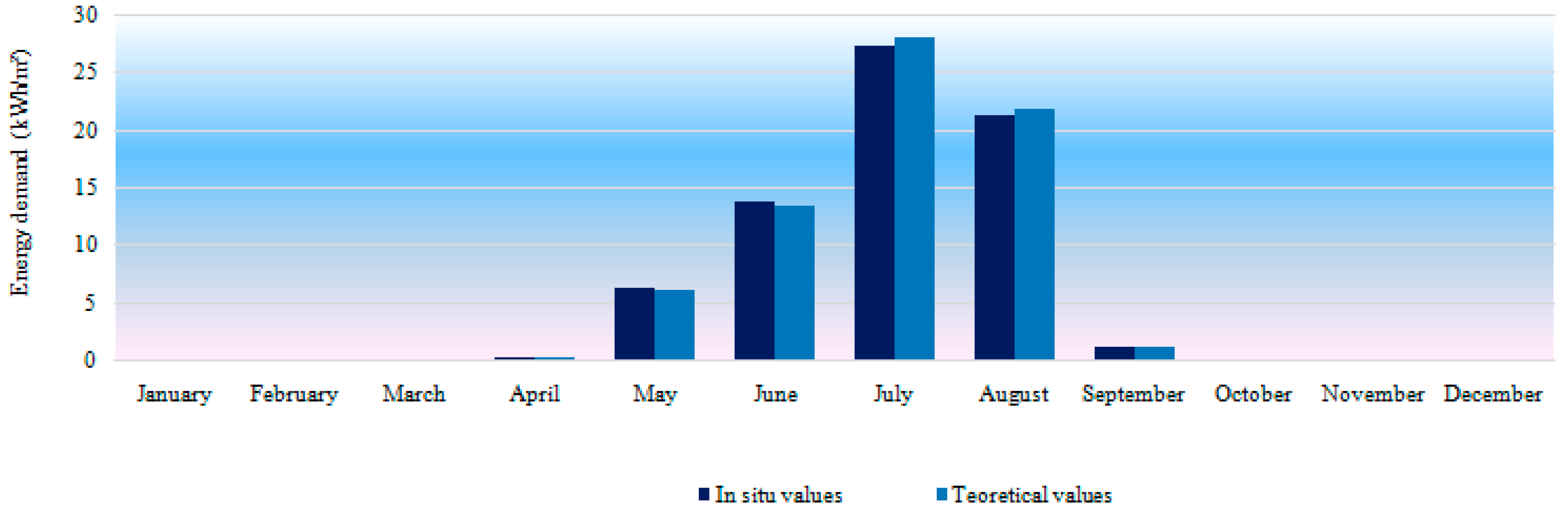
With respect to energy demand, there was a significant difference during the heating period, but for the cooling period, the differences were insignificant. In some situations, the energy demand is higher for case II, in which the real U and g values were used (during the cooling period) (Figure 6 and Figure 7).

4. Conclusions

The percentage difference between the two methods in case I was 18.91%, and the difference between the two methods in case II was 22.4% (

Table 7. Final results for the heating energy demand.

	Heating Energy Demand		Difference	M.U.	Percentage (%)
	Steady-State Method	Dynamic Method
Case I	134.87	109.37	25.5	kWh/m²year	18.91
Case II	119	92.34	26.66	kWh/m²year	22.40

).

The current study shows the differences resulting from modifications of the U and g values (i.e., theoretical vs. real values). Furthermore, our results highlight the differences between the heating energy demand obtained using the steady-state method and the dynamic method.

The heating energy demand values obtained using the real U and g values are slightly lower than those obtained with theoretical values. This difference occurs because the values obtained according to the Romanian Methodology undervalue the material thermal resistances.

The obtained in situ values can be applied in the case of existing buildings for which no data are available with respect to the elements of the building envelope; furthermore, in cases for which data are available, in situ values can be used for validation.

The differences between the two energetic calculation methods occur because the dynamic method uses variable climate parameters (i.e., temperature, wind and humidity), according to climate data recorded over a long period of time. Furthermore, in the dynamic method, the internal gains are highly detailed (in the present study, we considered internal gains from people and lightning equipment), considering the operating schedule for of building, whereas the dynamic method takes into account thermal inertia, i.e., the capacity of the building to store heat, as well as shadowing elements, which in the current study, were the building’s balconies and the neighbouring buildings. The steady-state method is a general method that assumes significantly higher values, although it is less time-consuming than the dynamic method because it does not require the building design.

The steady-state method using Doset-PEC is limited to the Romanian territory, as the program was developed according to the Romanian Methodology, whereas the dynamic method using EnergyPlus can be applied to any building in the world.

Every method has its advantages and disadvantages, and a methodology should be chosen according to the complexity of the project and whether significant material reductions are possible.