Evaluation of Machine Learning and Web-Based Process for Damage Score Estimation of Existing Buildings

Abstract

The seismic vulnerability assessment of existing reinforced concrete (RC) buildings is a significant source of disaster mitigation plans and rescue services. Different countries evolved various Rapid Visual Screening (RVS) techniques and methodologies to deal with the devastating consequences of earthquakes on the structural characteristics of buildings and human casualties. Artificial intelligence (AI) methods, such as machine learning (ML) algorithm-based methods, are increasingly used in various scientific and technical applications. The investigation toward using these techniques in civil engineering applications has shown encouraging results and reduced human intervention, including uncertainties and biased judgment. In this study, several known non-parametric algorithms are investigated toward RVS using a dataset employing different earthquakes. Moreover, the methodology encourages the possibility of examining the buildings’ vulnerability based on the factors related to the buildings’ importance and exposure. In addition, a web-based application built on Django is introduced. The interface is designed with the idea to ease the seismic vulnerability investigation in real-time. The concept was validated using two case studies, and the achieved results showed the proposed approach’s potential efficiency.

1. Introduction

Natural calamities can be unpredictable and may leave a cumbersome loss of life and economy. The infrequent seismic events (intermediate to large) eventually end up claiming lives and buildings or houses. The post-earthquake consequences are more evident in the metropolitan regions compared to rural areas. The complexities and unorganized distribution with inadequate design code implementation for mid-to-high-story buildings lead to unfortunate fatalities. In the past, significant earthquakes worldwide have provoked many human casualties and damages to structures. It reportedly killed 8519 persons and maligned 80,000 buildings in Nepal’s territory [1]. City Bam, in southeastern Iran, was hit by an earthquake measuring 6.3–6.6 on the Richter scale early Friday morning on 26 December 2003. It claimed 26,271 lives and 51,500 fatalities [2]. On 15 August 2007, an earthquake of 7.9 Richter caused enormous devastation in Peru and claimed 514 lives and 1090 injuries. The dead-to-injured ratio was 32% [3]. On 12 May 2008, Sichuan, in China, faced one of the deadliest earthquakes in the past 30 years with an 8.0 magnitude. The authorities confirmed the death of 69,170 people, 17,426 missing, and 374,159 injuries [4]. Haiti was knocked by a giant earthquake with a magnitude of 7.2 on the Richter scale on 12 January 2010. The event aroused massive mortal and material casualties, with 212,000 dead, 512,000 wounded, and 1,000,000 homeless [5]. Many studies and records infer that notable earthquake-related fatalities occurred due to damages to buildings which caused approximately 75% of deaths as a result of earthquakes in the past decades [6].

It is not feasible to conduct a comprehensive analysis for every structure in an urban metropolis. Thus, a fast screening technique to filter out and prioritize the building stocks with high degrees of vulnerability, also known as Rapid Visual Screening or RVS, is felt to be highly essential. RVS, recognized for its fundamental calculations, provides a quick and reliable approach for assessing seismic risk. RVS was created in the 1980s by the Applied Technology Council (USA) [7] to assist a wide range of people, including building authorities, structural engineering consultants, inspectors, and property owners. This approach was created to be the preliminary screening phase in a multi-step process of assessing seismic risk. Ozcebe [8] provides a valuable overview of RVS. When screening out high-risk construction stocks, this technique is fast, dependable, and efficient. For executing RVS, a sheet with preset criteria is considered and a qualified assessor implements a preliminary walk-down assessment to determine the damage grade of buildings. The process is followed by the evaluator taking note of physical characteristics such as overhangs and floating columns. First, a Basic Score (BS) is calculated using a formula and then allocated to the building following several international codes.

Throughout the last 25 years, many research projects have used artificial intelligence (AI) capabilities in earthquake engineering, such as methods based on machine learning (ML) and neuro-fuzzy [9,10,11]. The intrinsic capacity of ML to embed and deploy solutions of issues with known input data in order to extract predictions for the solution of the same kind of problems with unknown input data instantaneously led to the idea of using them for the approximation of the seismic damage status of existing structures in real-time following an earthquake.

The current study examines different ML methods for the rapid classifying of building damage grades through the rapid screening of a building. With the input dataset, many supervised learning approaches were investigated. The final classifier was created using the highest-scoring algorithm. Furthermore, the study was focused on the critical factors that cause probable loss following an earthquake. Despite the capabilities of AI approaches, there is a significant gap in adopting the most efficient technique for evaluating the seismic vulnerability of structures for which some possible reasons could be the substantial knowledge, the required skills, and the proper place for the application of an AI-based method [12].

2. Background of the Study

Earthquakes are the most devastating natural calamities that humans have witnessed [13,14]. Every year earthquakes claim thousands of lives [15] and cause significant loss in the economy (direct or indirect), massive fatalities, and suspension in occupancy as well as in business, not only in developing but also in the developed and scientifically well-established (particularly in earthquake engineering) countries [16,17].

In general, an estimation of any damage involves the complications of defining, assessing, and modeling the associated factors along with controlling the uncertainty. Engineering communities have the challenge of predicting the structures’ expected damages and face complexities, vagueness, and difficulties in their estimations [18], especially when it comes to dealing with a large building stock. Hence, restricting the damage to existing reinforced concrete (RC) buildings is emphasized, as they are more vulnerable than new buildings constructed according to the latest codes. The pre-earthquake assessment of existing structures has been introduced within the general framework of seismic risk management and aims to form a strategy for prioritizing buildings for further comprehensive analyses [19]. Although most new RC buildings fulfill the seismic safety criteria, many existing old RC buildings are not compliant with the principles of modern seismic codes, lacking ductility and sufficient seismic resistance, and hence their vulnerability analysis demands more attention. Lessons learned from the performance of buildings during previous earthquakes and research over the last three decades resulted in improved seismic design provisions and building resiliency [20,21]. The majority of the existing buildings are operational and require an assessment to analyze how safe they are to resist any seismic event in terms of life safety. A rapid and efficient risk-based seismic vulnerability assessment of existing buildings can help with estimating damage grades, prioritization for further analyses, saving time and costs, and assisting decision-makers with the provision of post-disaster crisis management plans [22].

2.1. Rapid Visual Screening

RVS estimates the seismic vulnerability of structures in a given territory. It depends on associations between the buildings’ evaluated seismic performance and architectural typology (frame, shear wall, monolith, in-fill), material (steel, RC, masonry, wood, composite), design methods implementation, and several other factors [23]. Additional inputs to the analysis include the level of earthquake hazards. The predictions are based on expert opinions, pushover analyses, compelling response studies, and the performance of similar buildings in past seismic events. The RVS methods allow for quantifying structural vulnerabilities more easily than analytical approaches [24] by filtering the weak structures through faster implementation. There is no need for detailed calculations and multiple scenarios. A scale-based or score-based system quantifies the likelihood of a building collapse, while the scale or score represents the possible damages after an earthquake [25].

2.2. Machine Learning in Seismic Vulnerability Assessment

AI methods provide a device or computer with the ability to imitate human intelligence (cognitive process), procure from events, adapt to the newest information, and perform human-like activities. These techniques accomplish tasks intelligently and accurately while keeping adaptive and productive for the entire system. Abundant literature is available that attempted to integrate various branches of AI from several areas with an RVS method. There is a broad set of techniques that come in the domain of artificial intelligence, including Artificial Neural Networks (ANNs), ML, Fuzzy Logic (FL), and Multilayer Feedforward Perceptron Networks (MFPNs). A comprehensive review of different AI techniques developed in the literature for the application of RVS to existing buildings and damage classification can be found in [26]. Morfidis and Kostinakis [27] applied an ANN to explore the number and combination of seismic specifications and help forecast the seismic damage caused to the RC buildings. The desired combination of parameters was between five and fourteen, while the Housner Intensity stood the most important among all. In 2018, Morfidis and Kostinakis conducted another study [28] using a model based on an MFPN. Several algorithms trained the model and using the Maximum Inter-Story Drift Ratio, the damage index of the earthquake was examined. In another study published by Morfidis and Kostinakis [12], the seismic vulnerability was evaluated using an MFPN. The model was trained via datasets obtained from a number of RC buildings in Greece with heights of 3–30 m. The study aimed to exchange the knowledge base between a civil engineer and an ANN expert.

In 2010, Tesfamariam and Liu [29] conducted a comparative study on different classification methods of the Neural Network (NN), namely Naive Bayes (NB), K-Nearest-Neighbor (KNN), Fisher’s Linear Discriminant Analysis (FLDA), Partial Least Squares Discriminant Analysis (PLS-DA), Multilayer Perceptron Neural Network (MLP-NN), Classification Tree (CT), Support Vector Machine (SVM), and Random Forest (RF). For different damage states including none (O), light (L), moderate (M), severe (S), and collapse (C), indicators 1, 2, 3, 4, and 5 were used, respectively. KNN and SVM performed optimally for segregating buildings with “Immediate Occupancy” (IO) and “Life Safety” (LS). A team of researchers (Zhang et al. [30]), in 2018, presented an analysis report on their approach based on ML. The selected mechanism was the Classification and Regression Tree (CART) and RF to sketch the response and damage patterns of buildings. They found an accuracy of 90% in predicting response patterns and 86% for both CART and RF. The traditional architecture of an ANN has each neuron connected to every other neuron, while a Convolutional Neural Network (CNN) has the last layer fully connected.

Harirchian et al. [21] utilized an optimized MLP-NN to study the earthquake perceptivity through six buildings’ performance variables which can help in obtaining optimal foresight of the damage state of RC buildings using an ANN. The MLP network was trained and optimized, utilizing a database of 484 buildings damaged in the Düzce earthquake in Turkey. The effectiveness of this recommended NN design was displayed through the achieved results to build an introductory estimation procedure for the seismic risk prioritization of buildings.

Another study conducted by Allali et al. [31] focused on an approach based on FL for the post-earthquake damage evaluation of buildings. They proposed the creation of the global damage level of buildings with different lateral load resisting components. More than 27,000 buildings damaged in the destructive 2003 Boumerdes earthquake in Algeria (M${}_{\mathrm{w}}$ = 6.8) were considered in the review process. The survey included the structural and non-structural components, and other factors such as soil conditions, etc., were overlooked. The damage levels of components and global damage levels were indicated using a scale system from “No damage” for D${}_1$ up to “collapse” for D${}_5$. The study applied a novel purpose of weighted fuzzy rules to associate the components’ damage levels to the global damage levels. The outcomes showed an accuracy of 90%.

ML represents a branch of AI that uses the essential components of illustration, evaluation, and optimization to generate forecasts using computational algorithms that improve with time. From a natural hazard risk evaluation perspective, SVM approaches have been frequently used [32,33,34,35]. Few researchers compared an SVM performance with other soft computing techniques or used an integrated approach that included the characteristics of two different methodologies. Gilan [36] used an SVM combined with a fuzzy evolutionary function (EFF-SVR) to predict the concrete compressive strength and compared their findings with ANFIS, fuzzy function with least square estimation (FF-LSE), ANN, and enhanced FF-LSE. Simulation results and comparisons showed that the suggested EFF-SVR technique outperformed other methods in terms of performance. In their research investigations on compressive strength predictions for the no-slump concrete and concrete with a significant volume of fly ash additive, Sobhani [37] and Sun [38] utilized SVM and least square SVM (LS-SVM) models, respectively, and compared them with ANN models. SVM and LS-SVM models were high-speed in both tests and helped overcome the ANN model’s disadvantages of over-training and poor generalization skills.

Harirchian [35] used a supervised ML methodology on the post-damage data of RC structures damaged by the 1999 Düzce earthquake in Turkey to develop a method applicable to risk assessment and crisis management strategies. They used an SVM optimization model to assess the efficacy of the suggested technique in damage prediction. The database contained 484 buildings, with 22 feature characteristics serving as inputs to the suggested method. When all 22 characteristics were used as inputs to the technique, their findings showed a 52% accuracy. The SVM technique has been used to estimate seismic risk for large-scale data. In fact, constructing a dataset with various parameters as inputs to an extensive computational model for many structures in an area rather than individual buildings would be a complicated task which would render the procedure computationally expensive. Zhang [39] fixed this problem by performing two case studies with 11 and 20 building features, respectively, utilizing an SVM as a data mining technique. For testing the performance and accuracy of the SVM in seismic vulnerability prediction in terms of spectral yield and ultimate points using capacity curves acquired by a pushover analysis [40,41,42,43] in individual as well as regional scales, samples were randomly selected from Taiwan’s National Center for Research on Earthquake Engineering (NCREE) [44] database of 5400 school buildings in Taiwan. Their results showed an average accuracy of 64% on an individual scale, which could be raised to 74% by increasing the number of samples used in the dataset’s training. A seismic risk assessment was completed on a regional scale when the SVM approach was combined with the seismic-demand curves based on building sites. Deep Neural Networks (DNN), also known as Deep Learning (DL), have been effectively employed in a range of applications [45], attracting the interest of academics since DL outperformed alternative ML approaches such as kernel machines [46,47,48].

Exposure models, or the inventory of people and facilities geographically separated at the regional scale impacted by earthquakes, are among essential variables that make up the fundamental inputs for a seismic risk assessment. Gonzalez [49] utilized a methodology that included deep learning and a CNN method, which was applied to Google Street View photos for image processing and categorizing individual buildings’ structural typologies, which was then used for exposure models and a seismic risk assessment. A dataset from 9989 structures across eight typologies in Medellín, Colombia, was taken into consideration. The results indicated that non-ductile structures are most vulnerable in an earthquake, with an accuracy of 93% and a recall of 95%.

3. Data and Methodology

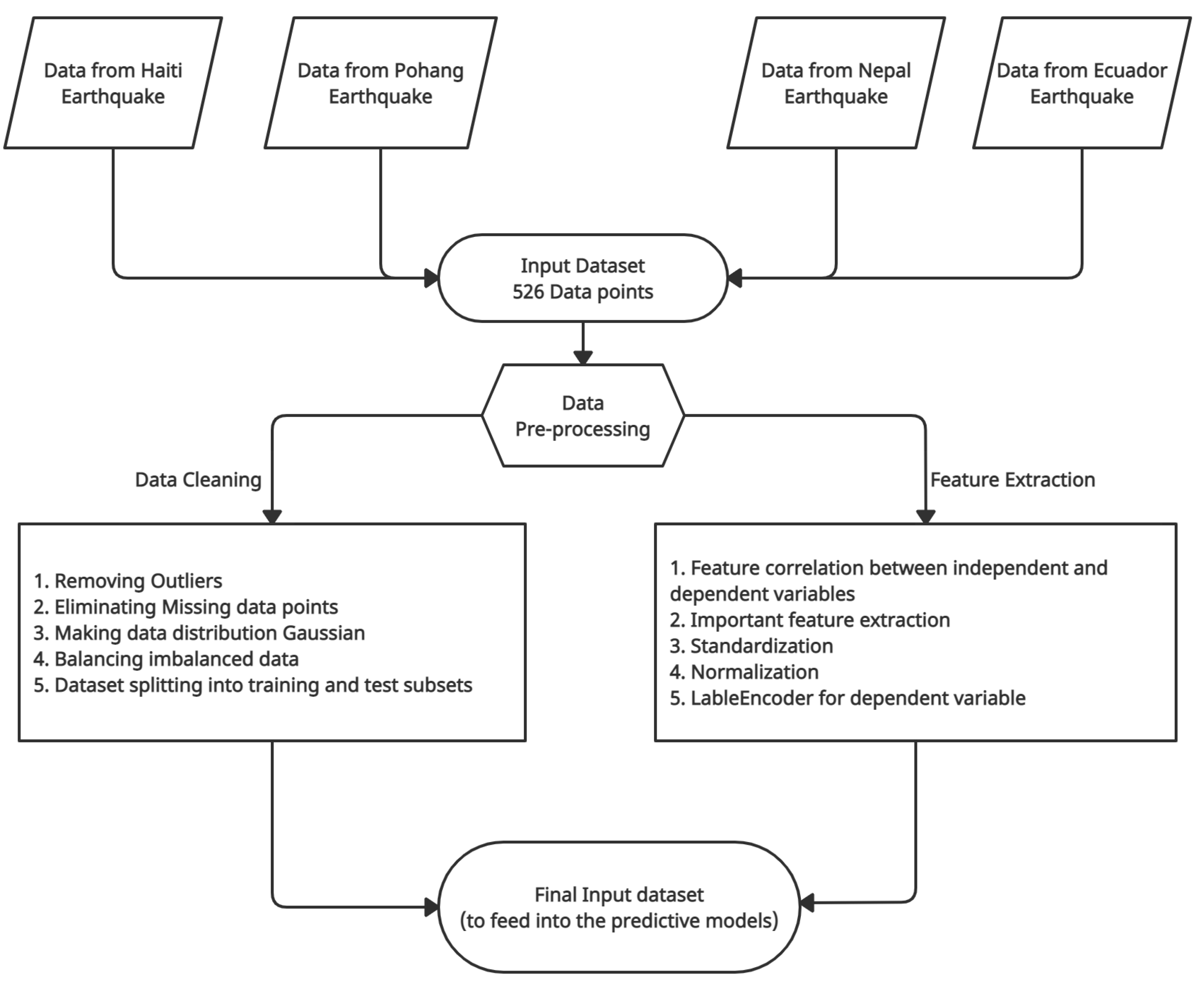
3.1. Input Data Source

Data are the observations of real-world phenomena, and they make the backbone of ML models. Data present a small window into a restricted viewpoint of reality. The accumulation of all of these observations provides a picture of the whole. However, it should be noted that even when one has a massive dataset, the adequate number of data points for some instances of interest might be pretty small.

The study presented in [50] incorporates cumulative data collected from RC buildings shaken under the past four seismic events in Ecuador, Haiti, Nepal, and South Korea. The data are archived in the open-access database of the DataCenterHub platform [51], simultaneously with the data obtained from the studies by different research groups on that platform [52,53,54,55]. Data from the individual earthquakes were not sufficient for predictive models to work efficiently. Therefore, to supplement the data and create a global method, the study consolidated all four datasets and merged them into one.

ML models require learning from data. ML algorithms acquire a mapping from input variables to a target variable on a predictive modeling project. In this study, the input dataset used for the predictive analysis consists of 526 data points corresponding to 8 independent building features and 1 dependent set of variables. The dependent variables in the dataset are the damage scales from 1 to 4 that have been assigned to the affected RC buildings after seismic events. The predictive models need independent and dependent variables in order to make predictions. In

Table 1. RC buildings’ input feature collected for RVS study (based on the conducted study in [21]).

Features	Unit	Type
No. of Stories	N (1, 2, …)	Integer
Total Floor Area	m${}^2$	Integer
Column’s Cross-Sectional Area	m${}^2$	Integer
Concrete Wall Area (Y)	m${}^2$	Integer
Concrete Wall Area (X)	m${}^2$	Integer
Masonry Wall Area (Y)	m${}^2$	Integer
Masonry Wall Area (X)	m${}^2$	Integer
Captive Columns	N (exist = yes = 1, absent = no = 0)	Binomial

, the buildings’ featured parameters, their relative units, and their category types have been presented. These features are the input variables for the given dataset, whereas the target or dependent variable contains the four damage scales, as shown in

Table 2. Damage scales associated with various risk factors.

Damage Scale	Risk Association
1	No visible damage to the structure. Safe to reoccupy.
2	Low damage. Hairline to wide cracks in the structural elements. Spalling of concrete may also be observed.
3	Significant loss. Failure of at least one element in the structure.
4	Severe damage. At least one floor slab or part of it loses its elevation.

, for defining the damage and risk associated with the corresponding RC building.

A feature depicts the numeric representation of raw data. The right features are essential to the task at hand and should be easy for the model to ingest. Feature engineering expresses the most appropriate features for the given data, model, and task. The number of features is also imperative. If there are not enough informative features, the model will not achieve the final goal. In case of many features or trivial features, the model will be more expensive and tricky to train. Something might go wrong in the training process that impacts the model’s performance. Features and models sit between raw data and the desired insights. Thus, in an ML workflow, not only the model but also features are equally important.

3.2. Data Preprocessing

ML algorithms cannot fit solely on raw data. Instead, the data should be transformed by preprocessing to meet the requirements of individual ML algorithms. Figure 1 shows various steps followed in the study including merging four different datasets to form one, processing the consolidated raw dataset for improvising it, and making the data suitable for feeding into the predictive models. The study used various libraries available in $Python$ programming language to preprocess the data and create ML predictive models. Data preprocessing is vast and can consist of numerous steps depending upon the data, features, and the model requirements. Below, sub-sections elaborate on the preprocessing steps carried on the raw dataset for implementation in the study.

3.2.1. Data Preparation

Data cleaning regards recognizing and fixing errors in the dataset that may negatively influence a predictive model. It is referred to all kinds of actions and activities which identify and adjust errors in the data [56]. One of the most common forms of preprocessing consists of a simple linear re-scaling of the input variables [57].

• Outlier detection—An outlier is a data point that is unlike the other data points. They are rare, discrete, or do not belong in some way. There is no definite technique to distinguish and recognize outliers as usual because of the specifics of each dataset. However, a domain expert can interpret the raw observations and verify if any given data are outliers or not. Identifying outliers can be tricky even after a thorough comprehension of the data. Proper attention should be taken not to eliminate or replace values rashly, specifically when the sample size is small [58].
  The input dataset for the study is medium size, so detecting the outliers on the basis of extreme value analysis was possible. There were few data points which were not in the range and distribution of attribute values. Those data points were eliminated to avoid creating any unforeseen circumstance to control the predicting model inaccurately.
• Missing data elimination—Major ML algorithms utilize numeric-type input data values arranged in rows and columns in a given dataset. Missing values in a dataset can create problems for the algorithms to function optimally. Therefore, it is a common practice to identify the missing values and substitute them with a corresponding numerical value. The method is known as missing data imputation or data imputing.
  A known approach for data imputation is replacing all missing values for that column with the respective column’s mean or median value. $Scikit$-$learn$ library provides a $SimpleImputer$ with a mean or median strategy for missing value elimination. The input dataset for this study is moderately tiny with only 526 values; however, there were 3 NaN (Not a Number) data points raising errors while processing the algorithms. Therefore, using the conventional strategy, those NaN were replaced by the mean value of their respective columns.
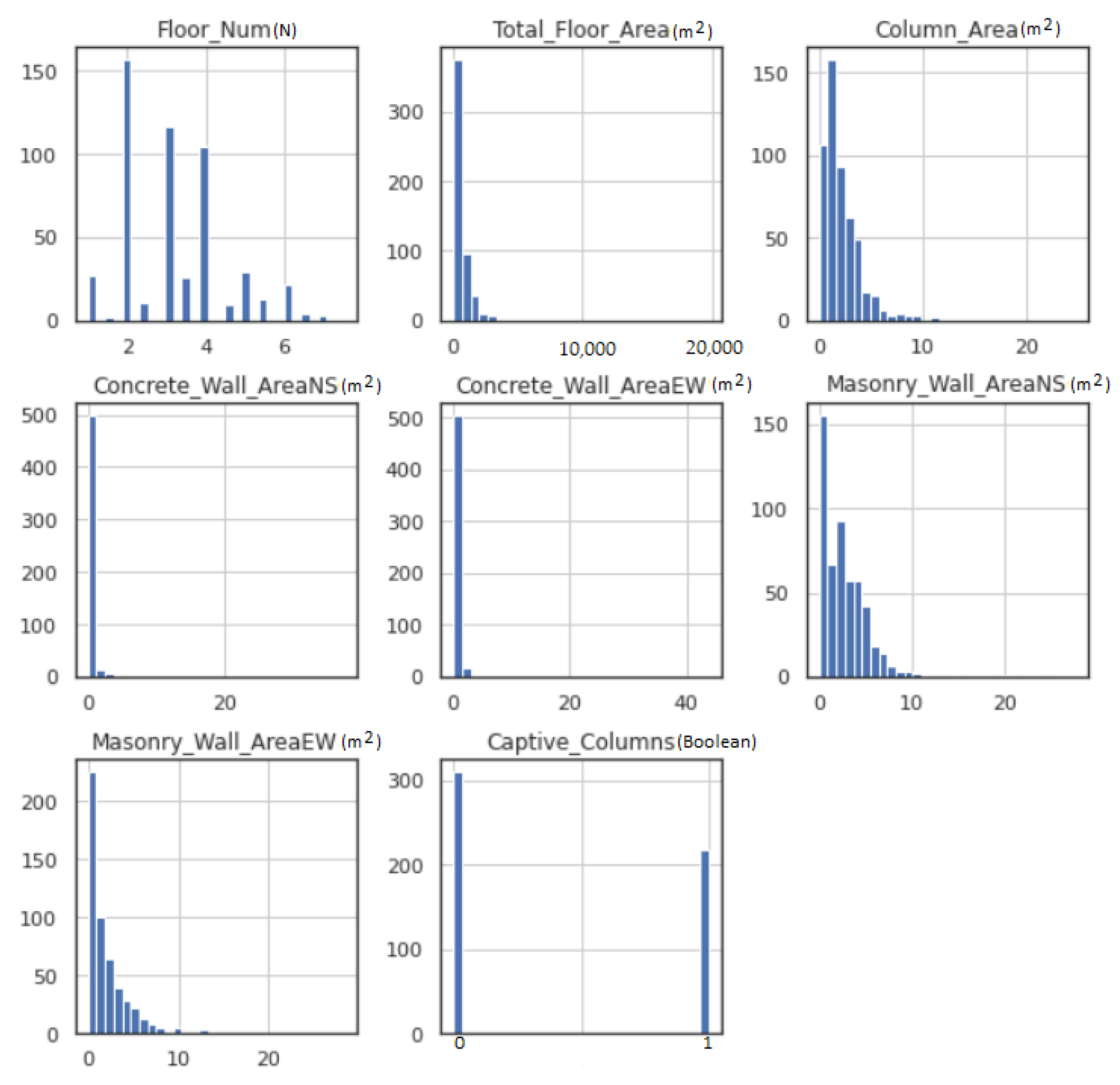
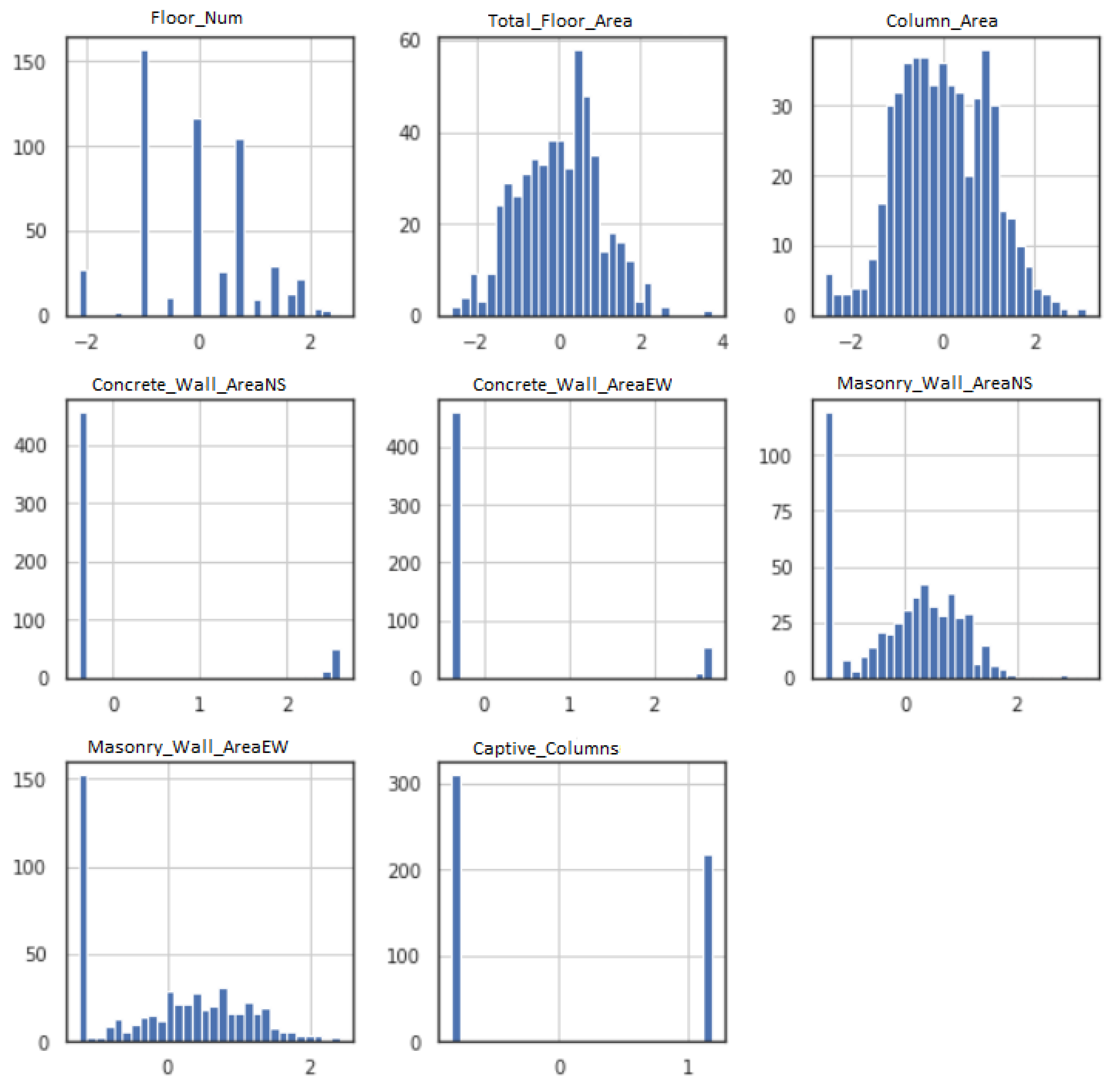
• Gaussian data—ML models function better when the data have Gaussian distribution. The Gaussian is a standard distribution with the familiar bell shape. Data fitting techniques can modify each variable to make the distribution Gaussian, or if not Gaussian, then more Gaussian-like. These transforms are most efficient when the data population is nearly Gaussian, to begin with, and is skewed or affected by outliers. Figure 2 shows the histogram for each feature input variable. Floor number has Gaussian-like distribution of the data points, whereas most of the features are skewed toward the left. The captive column obtained a binomial value (0 or 1); therefore, the data distribution is discrete.
  Figure 3 illustrates the data distribution for each feature input after employing Power-Transformer class from $Scikit$-$learn$ library. Total floor area and column area show a better Gaussian bell shape, whereas masonry wall area NS and masonry wall area EW have some skewness on the left side. Due to very few non-zero data points, the area of concrete wall area NS and concrete wall area EW did not show any significant improvement.
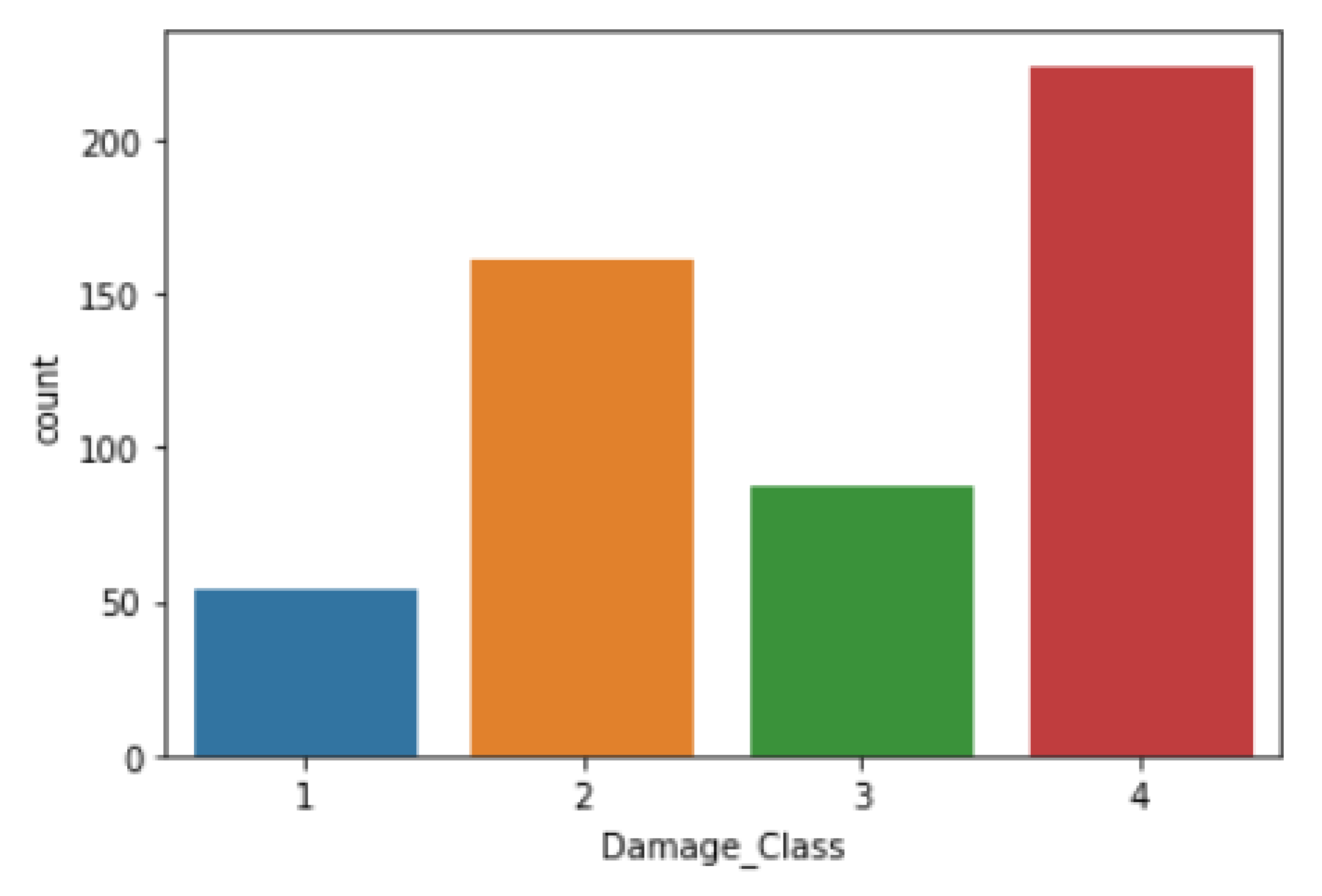
• Imbalanced Data—An imbalance in data distribution for each input feature creates objections for predictive modeling. In real-world cases, the dataset contains irregular data sharing several times, affecting the model prediction’s performance. Figure 4 depicts that the input dataset contains an asymmetric distribution of feature data which resulted in imbalanced data in each output class. For example, damage class 4 has the highest number of samples, whereas damage class 1 has the least. This kind of data distribution prevents the model from performing optimally. Synthetic Minority Oversampling Technique (SMOTE) [59] generates synthetic data for the minority class, therefore producing symmetry for majority of classes.

  Table 3. Balanced number of data in target variable with SMOTE [60].

  Target Class	Imbalanced Data	Balanced Data
  1	54	224
  2	161	224
  3	87	224
  4	224	224

  illustrates that, using SMOTE, the imbalanced state of data distribution in the target variable is balanced.
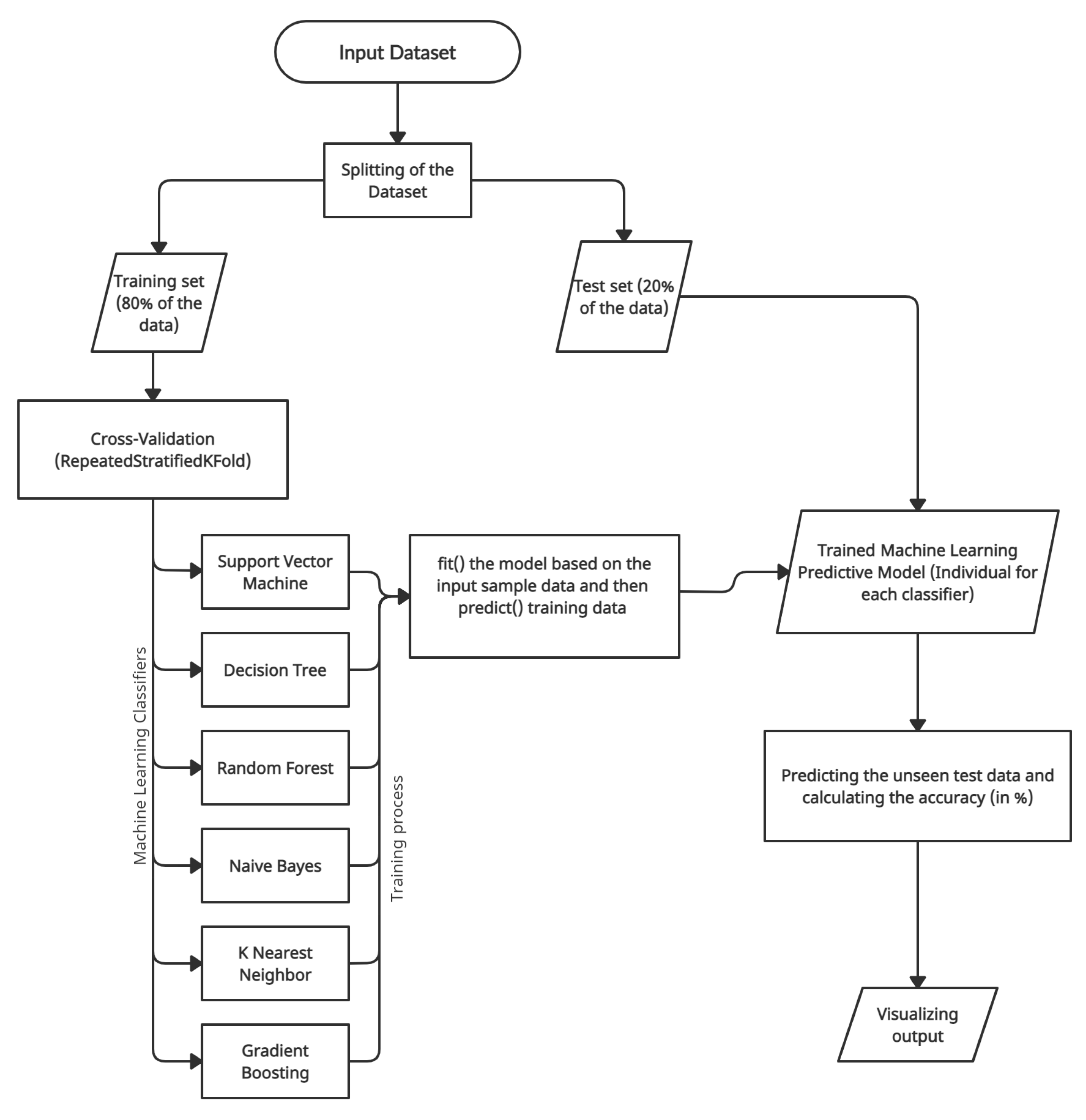
• Dataset splitting—The suitable approach for performing data preparation with a train–test split evaluation is to fit the data preparation on the training set, then apply the transform to the train and test sets. Therefore, the input dataset was split into (80–20%) into the training set and testing set using function $train$-$test$-$split$ from $model$-$selection$ module in $Scikit$-$learn$.
• Cross-Validation—As a good practice, ML models should evaluate the dataset using k-fold cross-validation, particularly in small to medium-sized datasets. Cross-validation aims to examine the model’s worth to predict unseen data, check issues such as model overfitting, or biasedness to give an insight into the model behavior against an independent dataset. The study implemented repeated stratified 10-fold cross-validation using the function RepeatedStratifiedKFold from module ensemble in $Scikit$-$learn$.

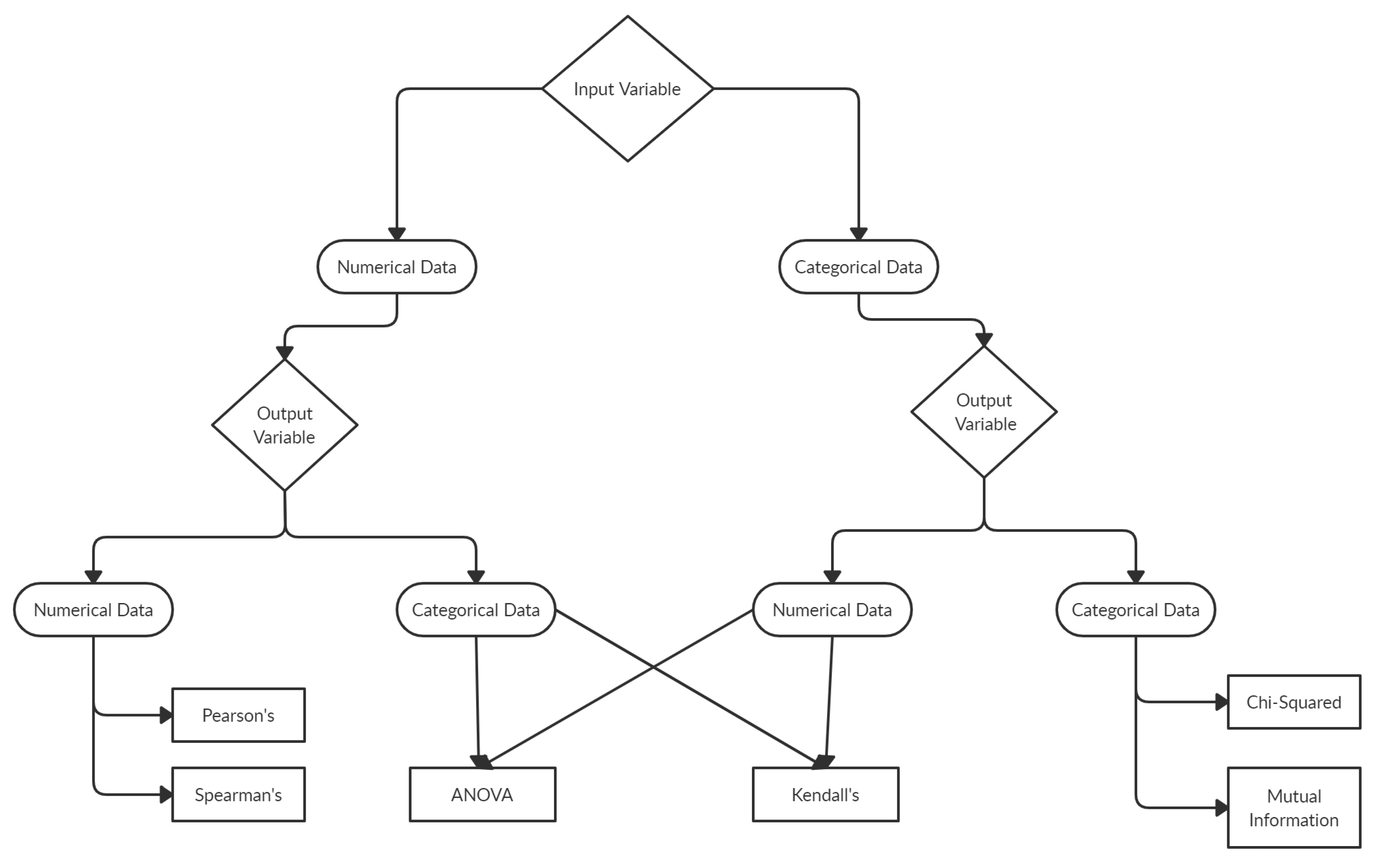
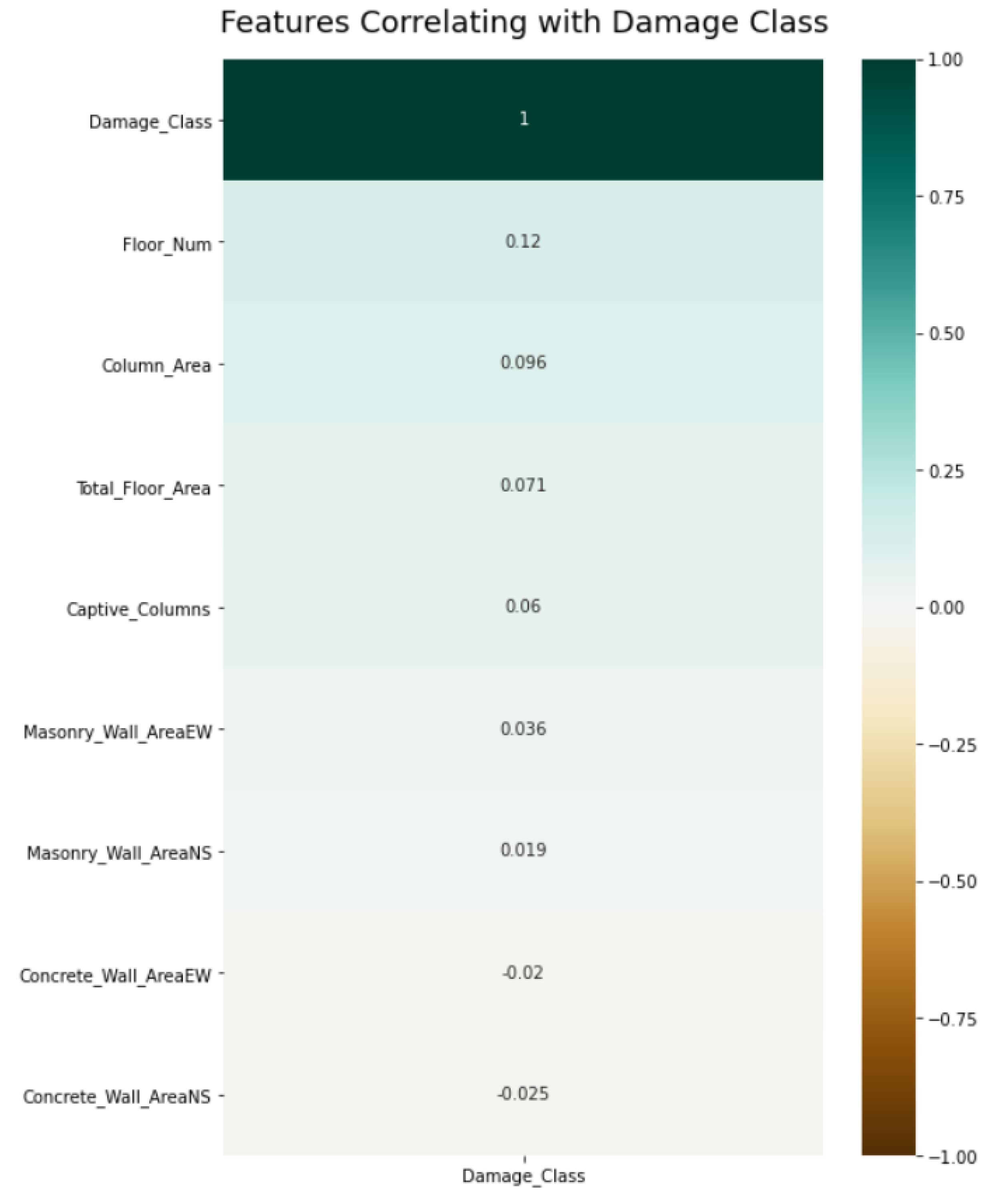
3.2.2. Feature Selection

Feature selection limits the number of independent variables in an input dataset while creating a predictive model. Reducing the number of input variables helps in terms of reducing the computational cost of modeling and also in order to increase the model’s performance.

Figure 5 shows the application of statistical measures to draw a correlation between independent and dependent variables as the basis to filter out feature selection. For the available dataset, where the independent/input variable was numerical and dependent/output variable was categorical, ANOVA method was implemented to extract the essential features out of all given parameters.

3.2.3. Data Transformation

ML models are mapped from input variables to an output variable based on a suitable pre-defined algorithm. Variations in the scales over independent variables may raise the complexity of the problem to be modeled. Following approaches transform the data in a proportionate scale to achieve the optimum output.

• Standardization—Standardization of a dataset includes re-scaling the spread of values such that the mean of observed values is 0 and the standard deviation is 1. The method is offered by a function called $StandardScaler$ available in the $preprocessing$ module of $Scikit$-$learn$ library. Deducing the mean value from the given data is known as centering, and dividing the data by the standard deviation is known as scaling. The method is also referred to as center-scaling.
• Normalization—Data points in any dataset may scale differently from variable to variable. Often ML predictive models perform better if the variables are scaled in a standard range, for example, in the range between 0 and 1. The scaling of all variables in the range between 0 and 1 is known as Normalization. Class $MinMaxScaler$ from $preprocessing$ module in $Scikit$-$learn$ library normalizes the input variable.
• Label Encoder—ML predictive models assume all the provided input and output variables to be numeric. Numerical data include data points that comprise numbers, such as integer or floating-point values. Categorical data involve label values instead of numerical. Categorical variables are frequently known as nominal. $Scikit$-$learn$ library also has this requirement which implies that all categorical data must be transformed to numerical values.
  For the dataset applied in this study, the target variable is in the categorical form: the different damage classes assigned to the earthquake-affected RC buildings. With the one-hot encoding method, the categorical output variable can be changed to an ordinal numerical form. The ordinal encoding transform is available in the $Scikit$-$learn$ library via the $OrdinalEncoder$ class.

3.3. Predictive Model Building

Designing an ML model involves several steps, as demonstrated in Figure 6. After preprocessing, the input dataset (including the five feature input parameters) is split into training and test subsets in a proportion of 80 and 20%, respectively. The training subsets underwent cross-validation, which further divided the training set into smaller training and validation subsets. In the study, there are ten subsets of the training data. There are six popular ML classifiers implemented: SVM, DT, RF, NB, KNN, and GB. While nine training subsets’ data were training each classifier, the validation set evaluated the classifier’s performance by reviewing their precision for each output class. Unlike binary classification [61], there is no positive or negative class in a multi-class classification problem, which means, in the case of binary classification, the focus is on a positive class to detect; however, in a multi-class classification problem, each sample needs to be categorized into 1 of N different classes. Nevertheless, factors such as true positive (TP), true negative (TN), false positive (FP), and false negative (FN) are available in multi-class classification help in calculating the Precision, Recall, and F1-score, which are helpful in determining the performance of the classifiers. Below, equation shows the details of each keyword:

• $Precision=TP/(TP+FN)$
• $Recall=TP/(TP+FN)$
• $F1\text{-}score=2\times \left(\right(Precision\times Recall)/(Precision+recall\left)\right)$

To evaluate the classifier for general purposes, the model is exposed to the unseen test data. The accuracy was computed based on the model’s predicting capability. The results could also be visualized using different plots such as a confusion matrix.

Figure 6. Machine-learning-model building schematic flowchart.

Figure 6. Machine-learning-model building schematic flowchart.

3.3.1. Support Vector Machine

SVM was introduced through a statistical research learning theory [48]. A generalized case study [62] published using SVM showed that data are not linearly separable. Gärtner et al. [63] introduced the technique of handling multi-instance learning problems using regular single-instance learners to summarize bag-level data combined with SVM.

The study implemented a GridSearchCV function from model_selection module in the $Scikit$-$learn$ library for implementing the SVM algorithm with all the possible hyperparameters. The optimal accuracy achieved by the grid was 52% for the training data prediction and 57 % for the test data prediction using the hyperparameter values of C = 10, gamma = 1, and kernel = RBF.

3.3.2. Decision Tree Classifier

Developing a tree to classify samples from the training dataset is the goal of the decision tree algorithm, which is also known as Classification and Regression Tree (CART) [64]. The tree can be considered as a division of the training dataset, with samples progressing down the tree’s decision points until they reach the tree’s leaves, where they are assigned a class label. It follows the approach of “divide-and-conquer” to a set of independent instances.

This research analyzed the given input dataset with the DT algorithm while using $entropy$ as purity criteria and made the tree with a maximum depth of three. The trained model achieved 47% accuracy for the training set, while it evaluated the test data with an accuracy of 42%.

3.3.3. Naive Bayes

Determining the conditional probability of a class label that is provided with a data sample can be regarded as the problem of classification predictive modeling. The Bayes Theorem [65] provides a systematic method for estimating this conditional probability, but it is computationally expensive and requires many samples (a huge dataset). In the current study, Gaussian NB fits well as the attributes contain continuous values, and it was assumed that the data associated with each class have a Gaussian distribution. As a result, the model achieved 43% accuracy for the training set and 42% accuracy for the test set.

3.3.4. K-Nearest Neighbor

Proposed by Evelyn Fix [66] in 1951 and further modified by Thomas Cover [67], KNN is a simple non-parametric procedure in ML that is used for classification and regression problems. It is assumed that the same class data will remain close to each other, and the data will be assigned to a specific class with the most votes from their neighbors. Because the classification is locally approximated, it is also known as lazy learning. For the present dataset, KNN performed fairly good where it scored 64% accuracy for the training data, whereas for the test data, the accuracy was 45%.

3.3.5. Random Forest

RF is an ensemble classifier that originates from a significant advancement in DT variance. Each tree uses bagging and feature randomization to construct an uncorrelated forest of trees whose committee prediction is more accurate than that of any individual tree. Leo Breiman [68] proposed the idea, which combined concepts from bagging [69] and random feature selection by Ho [70,71] and Amit and Geman [72,73]. RF classifier attained almost equal accuracy for the training and test subsets for the given dataset, i.e., 45 and 37%, respectively.

3.3.6. Gradient Boost

GB follows ensemble learning by sequentially building simpler (weak) prediction models, with each model attempting to identify the error issued over by the previous model. Interestingly, because the loss function is optimized using a gradient descent, it is referred to as GB. GB employs a short, simpler DT, which makes it GBDT. It combines many weak learners to form one strong learner. Trees are linked in a series, and each tree attempts to minimize the error of the previous tree. GBDT has efficiency, accuracy, and interpretability features [74], and it is a popular ML ensemble algorithm. In addition, GBDT delivers high performance in a variety of tasks, including multi-class classification [75,76], click prediction [77], and learning to rank [78].

For the input dataset in this research, GBDT scored 78% on the training dataset and 51% on the test dataset. The outcome of the prediction is shown is Figure 7. The confusion matrix represents the classifier’s outcome on test data. Overall, GBDT classifier evaluated moderate numbers of true positives for class 2, class 3, and class 4, whereas, for class 1, it achieved the highest numbers of correct predictions.

3.4. Selection of ML Classifier

The models’ accuracies were recorded to evaluate their performance on datasets before and after the preprocessing steps. Before preprocessing, the dataset contained eight parameters, including floor number, column’s cross-sectional area, total floor area, existence of captive columns, masonry wall area in east–west, masonry wall area in north–south, concrete wall area in east–west, and concrete wall area in north–south, respectively.

Table 4. Accuracy scored by candidate classifiers with training and test subsets before and after postprocessing of raw dataset.

ML Classifier	Dataset (before Preprocessing)		Dataset (after Preprocessing)
	Training Set(in %)	Test Set (in %)	Training Set (in %)	Test Set (in %)
Decision Tree	48	41	47	42
Gradient Boost Decision Tree	77	49	78	51
K-Nearest Neighbor	64	46	64	45
Naive Bayes	46	35	43	42
Random Forest	38	33	45	37
Support Vector Machine	57	45	52	47

represents the accuracy (in %) scored by each of the trained classifiers on the set of training and test data before and after preprocessing of the dataset. GBDT performed good in comparison to all other classifiers.

Based on the performance of each candidate classifier on the test set, GBDT fits best for further creation of the browser-based application for rapid screening of RC buildings. Compared to other non-parametric models, ensemble models are robust and accurate because of their architecture, as shown by the performance of GBDT. However, a single DT is likely to overfit. Therefore, the classifier with a combination of DT models is preferred to reduce the chances of overfitting. These combined models are more efficient in terms of accuracy, as it can be seen for RF. To create an ensemble, RF employs a technique called $bagging$ to merge multiple DTs. Combining in parallel a number of DTs is called bagging, while processing them in a series is referred to as boosting. Boosting is the process of successively connecting weak learners to produce a strong learner. The weak learners in the GBDT model are DTs. Each tree tries to decrease previous mistakes and boost the accuracy and efficiency of the method. Figure 8 shows the working principle behind the GBDT classifier, as stated above.

3.5. Web-Development Using ML Model

One of the aims of this study is to incorporate the best-performing ML model in a browser-based UI. The purpose is to evolve from the traditional RVS methods to develop a fast, easily accessible, accurate, and scalable technique that can efficiently minimize the seismic risk assessment and reduce any imprecision that comes with human interference. Django is a free web framework based on Python language [79] that allows creating tested, scalable [80], and reliable online applications. Adrian Holovaty and Simon Willison created Django in 2003 for the Lawrence Journal-World newspaper, and it was freely distributed under the BSD license in 2005.

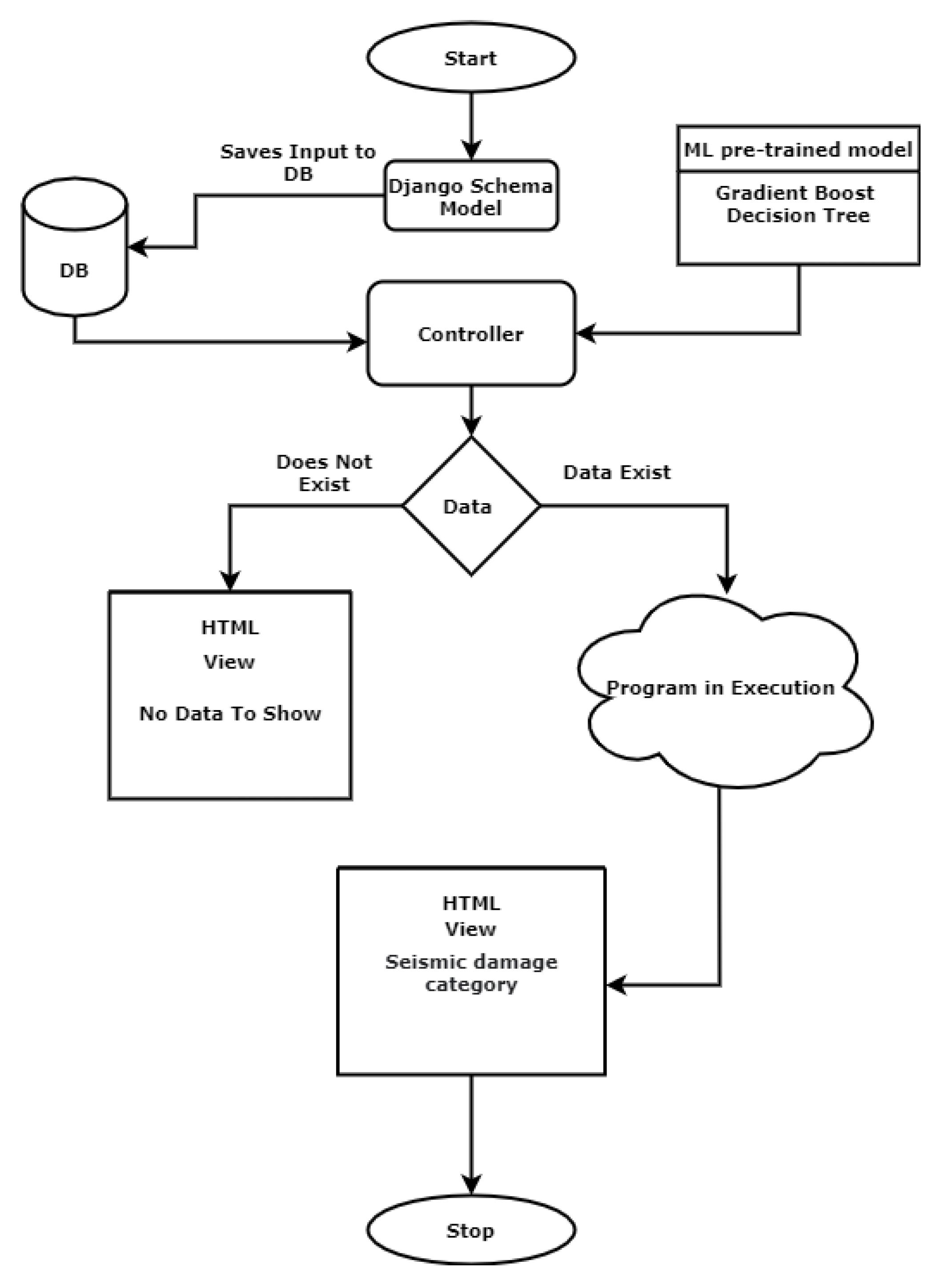
3.5.1. Design Approach

This section will introduce the design and implementation of the web application based on Django as defined in the previous section. First, the models require to be trained by the given input data. The data would be labeled in the case of supervised learning models [81] and unlabeled for unsupervised learning models [82]. Nevertheless, most of these models demand different amounts of data, depending on the algorithm, to reach a desired level of accuracy. After the model has been trained and is ready to predict, it will be given new and previously unseen data as input to make predictions about the target or independent variable in the second phase. Once the model is trained, the next concern is to utilize it in the web application to make predictions based on the unseen data that the user will feed. The trained models have acquired the state of a set of attributes that need to be kept in the application to predict the unseen data.

The GBDT is trained outside of the web application by the training dataset. Dataset is cleaned before training phase by preprocessing, and the model’s performance has been recorded in terms of accuracy by the test data. Figure 9 represents the correlation coefficient of each attribute in the dataset for each given target class. Based on the outcome, the following five attributes have the highest predictive ability to predict the seismic vulnerability of any RC building.

Figure 10 describes the flow of the process in Django architecture. The Django Schema Model (or Model) defined the fields for the input attributes to save in the database. The right side has the pre-trained ML model feed to the logic layer; controller or View. Based on the provided rules from the ML model, the controller will perform and pass the data to the appropriate Template. If there is no input data from the user, the Template will not show any prediction, but the data will be executed if there are valid data. The predicted damage class of the building will be displayed in the Template.

3.5.2. Project Structure

The project is divided into two main applications to separate concerns for different responsibilities across the project. The web-interface created is not hosted online; however, Github links are present to take a reference of the code and further contribute to it. The link for developing the classifiers is available at https://github.com/vandana1145/MasterThesisProjectCode/tree/feature/branch (accessed on 3 April 2022), and the Django code for the web-interface is linked at https://github.com/vandana1145/MasterThesisProjectWeb/tree/master (accessed on 3 April 2022). Figure 11 shows the sample index page of the web application. The web-based application developed for this research has the below main sections:

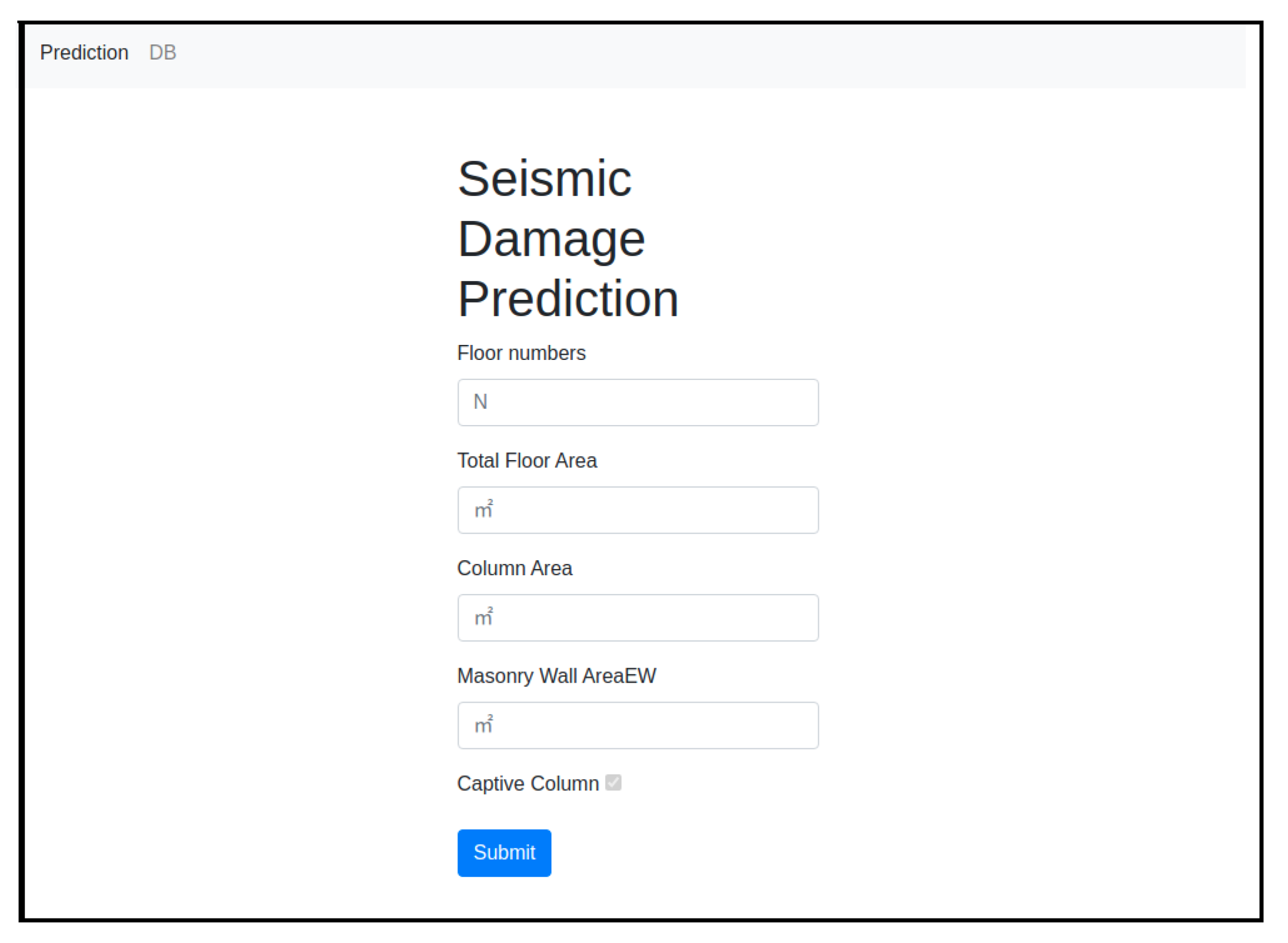
• Home Page: This application provides the basic home view of the project. The user can see the blank input fields to fill the values of required attributes.
• Predictor: The Submit button will have the functionality to use the ML model and to generate predictions.
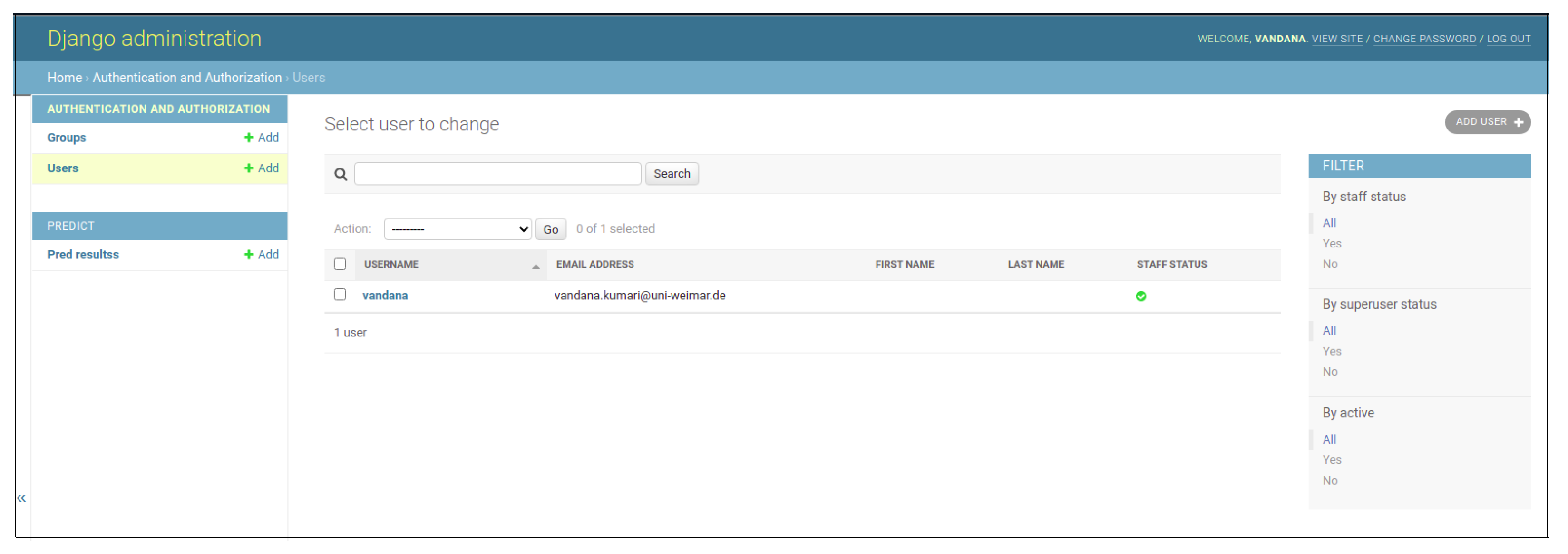
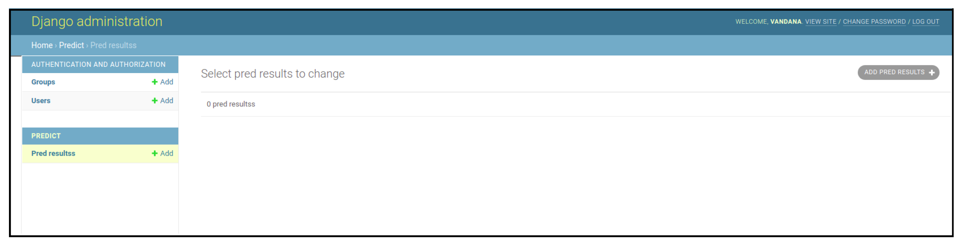
• Database (DB): The database or DB button on the home page will connect to another page where all the user-inserted inputs with their predicted values will be saved. In case of no data, the database table will show a blank page.

Modern websites come with a web-based administration backend as standard. Trusted site administrators can utilize the administrative interface or admin to create, update, and publish content, manage site users, and conduct other administrative activities.

Django includes a built-in administration interface. Django’s admin allows authenticating users automatically, showing and managing forms, and validating data. Django also has a user-friendly interface for managing model data. Figure 12 shows the screenshot for the admin page. As an example, one admin is registered for the site.

Figure 11. The home page with input fields and the submit button.

Figure 11. The home page with input fields and the submit button.

Figure 12. Django admin page.

Figure 12. Django admin page.

Once the model in Django is defined, the admin application interface can populate the GBDT model table in the database. The admin application is accessible by reaching this URL: “localhost: 8000/admin”. Figure 13 shows the “Pred results” in the admin panel.

4. Results and Discussion

In past years, there have been substantial improvements in the design codes and safety measures of modern buildings. However, existing RC buildings which do not satisfy code-based design criteria are in danger of severe damages under future seismic events. Consequently, an efficient, rapid, and reliable approach is of crucial importance to assess the seismic vulnerability and risk levels of a large stock of such buildings in a reasonable timeframe which can directly enhance post-disaster crisis management plans.

An ML model for estimating the post-earthquake structural safety assessment is created by integrating ML methods with an input dataset comprising 526 data points and four damage classification scales. The response and damage patterns are mapped to their categorized structural safety states using ML techniques such as DT, GBDT, RF, NB, KNN, and SVM. The predictor space is iteratively partitioned to capture the underlying connection. The predictive models reported in this study, trained using ML techniques, can make moderately accurate, sensitive, and specific predictions. When applied to response patterns with unknown safety states, the highest prediction accuracy is 57% for GBDT. A trained GBDT classifier was incorporated into a web tool based on the Django framework.

The proposed approach is applied to two case studies. Because there was no separate exclusive dataset to examine the performance of the classifier, the test was performed on several data points from available datasets of the Nepal [52] and Pohang [53] earthquakes. The tool was examined, and the obtained predictions were recorded as shown in

Table 5. Tested Predictions based on Nepal Earthquake Data.

Target Class	Number of Data Predicted	Correctly Predicted Data	Accuracy (in %)
1	7	2	28.57
2	7	4	57.14
3	7	2	28.57
4	7	5	71.40

and

Table 6. Tested Predictions based on Pohang Earthquake Data.

Target Class	Number of Data Predicted	Correctly Predicted Data	Accuracy (in %)
1	7	3	42.85
2	7	4	57.14
3	7	1	14.28
4	7	4	57.14

for the seismic data of the Nepal and Pohang earthquakes, respectively.

There were seven data points selected from each damage class for this study. In the case of the Nepal earthquake, the tool predicted class 4 with a higher accuracy than other damage classes. The only two true positives are for class 1 and class 3. Similarly, for the Pohang earthquake, there were seven input points for each target class. Here, the classifier predicted four true positives for class 2 and five true positives for class 4. Only one correct prediction occurred for class 3.

Building damage assessment is time-consuming and challenging due to the geographical dispersion of effects in an earthquake-affected area. The proposed technology might allow for quick evaluations of seismic damages. However, depending on the technique employed for the assessment, forecasting the spatial distribution of building damage with fair accuracy may vary.

The technique’s performance was estimated based on the case study results accomplished in the previous section. Therefore, one can interpret that the tool is fairly robust. However, although the realized model predicts with more than 50% accuracy, the performance has to be validated for utilization of the tool on a more extensive scale and in real-time.

5. Conclusions

There are existing RC structures which do not satisfy the code-based design and strength criteria and hence are not code-compliant. These structures are vulnerable to significant damages in the case of the next moderate to severe seismic events. Several factors contribute to seismic vulnerabilities of such buildings, including the application of obsolete building codes, poor design procedures, and non-standard construction techniques. The majority of these old RC buildings are still in use; therefore, the application of a rapid, efficient, and reliable seismic vulnerability assessment is of vital importance. This study has tried to integrate some of the most modern soft computing techniques with the traditional RVS methods to achieve a more enhanced rapid risk-based analysis methodology. The literature has demonstrated promising capabilities of soft computing techniques in achieving high levels of performance for solving a variety of intricate problems. The application of these methodologies to RVS techniques for the rapid vulnerability assessment of existing buildings can substantially minimize the subjectivity of evaluators, uncertainties, and vagueness and increase accuracy. Following an earthquake, the proposed framework in this research may be used to make a quick probabilistic evaluation of whether a damaged structure is safe to reoccupy. In addition, the model created by the ML algorithms may be used to prioritize field inspections after an earthquake. Furthermore, the probabilistic safety state forecasts might be employed in community resilience assessments to examine and improve the life-cycle performance of individual buildings.

A web development framework was necessary in order to construct the web application for the purpose of this study. Django was an appropriate choice because Python has widely been applied to analyze and process the datasets for constructing ML models. There are open-source and robust web development frameworks based on Python. A GBDT-trained model was implemented into a web browser-based simple application using the Django framework. The obtained results confirmed that the proposed approach for a rapid and inexpensive vulnerability assessment can be conducted. Information on seismic zone hazards is essential to extend the developed tool to other regions. Meanwhile, the more data are available, the more satisfactorily the ML technique converges statistically.

Nevertheless, the results emphasize that ML could be an exciting alternative in making a support tool for evaluating the vulnerability of buildings. Indeed, further investigations by increasing and diversifying the type of construction in the learning state could strengthen this last conclusion. Despite these limitations, this work has demonstrated the enormous potential of AI methods for the identification of vulnerable structures, decreasing future seismic hazards, and assisting decision-makers in post-disaster crisis management plans with direct outputs of saving time and costs.

Future Recommendations

This study covered a literature review of existing RVS methods for the vulnerability assessment of buildings and examined the integration of ML techniques with the traditional RVS to enhance its capabilities. Moreover, a web-based application was designed using the Django library of Python for the purpose of this research. Future investigations are necessary to validate the application of the proposed web-based tool to extend its utilization to other regions of the world, taking into account the seismicity characteristics and available seismic data in a given zone. Several recommendations for future research are given below:

• Future studies should consider additional data taking into account the structural system, scale, and damage classifications. In addition, the overall accuracy and robustness of prediction models can be enhanced in future research by adding more extensive datasets (e.g., numerous incidents) and additional site- (e.g., soil conditions) and building-specific predictor variables.
• Concept drift [83] is an ML phenomenon that focuses on data changes, resulting in the ML model’s testing performance to deteriorate over time. Finally, in the case of RVS, a model’s incorrect forecast might be dangerous as, over time, its performance may decrease. However, this effect can be checked by constantly updating the model and periodically re-fitting the model with new data. Therefore, in the long term, the effect of the concept drift needs to be addressed in any ML-based methodology.
• The web-based application is built in a test-driven development environment. The application is based on the Django framework and uses an internal WSGI gateway and an SQLite3 database. The server and database must be uploaded to the proper server and databases expressly developed for production environments. For heavy-load traffic settings, open-source servers such as Apache and Nginx can be utilized. Other open-source databases, such as MySQL, offer greater security and a broader range of features in a production setting. These ideas will need further research and experimentation, which will be left to future projects.

References

1. Dixit, A.; Shrestha, S.; Parajuli, Y.; Thapa, M. Preparing for a Major Earthquake in Nepal: Achievements and Lessons. In Proceedings of the 12th World Conference on Earthquake Engineering, Lisbon, Portugal, 24–28 September 2012. [Google Scholar]
2. Emami, M.J.; Tavakoli, A.R.; Alemzadeh, H.; Abdinejad, F.; Shahcheraghi, G.; Erfani, M.A.; Mozafarian, K.; Solooki, S.; Rezazadeh, S.; Ensafdaran, A.; et al. Strategies in evaluation and management of Bam earthquake victims. Prehospital Disaster Med. 2005, 20, 327–330. [Google Scholar] [CrossRef] [PubMed] [Green Version]
3. Doocy, S.; Daniels, A.; Aspilcueta, D.; Zambrano, P.; Rodriguez, S.; Hanif, H.; Shepard, S.H.; Milch, K.; Diaz, A.; Gorokhovich, Y.; et al. Mortality and injury following the 2007 Ica earthquake in Peru. Am. J. Disaster Med. 2009, 4, 15–22. [Google Scholar] [CrossRef] [PubMed]
4. Nie, H.; Tang, S.Y.; Lau, W.B.; Zhang, J.C.; Jiang, Y.W.; Lopez, B.L.; Ma, X.L.; Cao, Y.; Christopher, T.A. Triage during the week of the Sichuan earthquake: A review of utilized patient triage, care, and disposition procedures. Injury 2011, 42, 515–520. [Google Scholar] [CrossRef] [PubMed]
5. Gamulin, A.; Villiger, Y.; Hagon, O. Disaster medicine: Mission Haiti. Rev. Med. Suisse 2010, 6, 973–977. [Google Scholar]
6. Stein, S.; Geller, R.J.; Liu, M. Why earthquake hazard maps often fail and what to do about it. Tectonophysics 2012, 562, 1–25. [Google Scholar] [CrossRef]
7. Federal Emergency Management Agency. Rapid Visual Screening of Buildings for Potential Seismic Hazards: Supporting Documentation; Government Printing Office: Washington, DC, USA, 2015.
8. Ozcebe, G.; Yucemen, M.S.; Aydogan, V. Statistical seismic vulnerability assessment of existing reinforced concrete buildings in Turkey on a regional scale. J. Earthq. Eng. 2004, 8, 749–773. [Google Scholar] [CrossRef]
9. Alvanitopoulos, P.; Andreadis, I.; Elenas, A. Neuro-fuzzy techniques for the classification of earthquake damages in buildings. Measurement 2010, 43, 797–809. [Google Scholar] [CrossRef]
10. Xie, Y.; Ebad Sichani, M.; Padgett, J.E.; DesRoches, R. The promise of implementing machine learning in earthquake engineering: A state-of-the-art review. Earthq. Spectra 2020, 36, 1769–1801. [Google Scholar] [CrossRef]
11. Lazaridis, P.C.; Kavvadias, I.E.; Demertzis, K.; Iliadis, L.; Vasiliadis, L.K. Structural Damage Prediction of a Reinforced Concrete Frame under Single and Multiple Seismic Events Using Machine Learning Algorithms. Appl. Sci. 2022, 12, 3845. [Google Scholar] [CrossRef]
12. Morfidis, K.; Kostinakis, K. Use of Artificial Neural Networks in the R/C Buildings’ Seismic Vulnerabilty Assessment: The Practical Point of View. In Proceedings of the 7th ECCOMAS Thematic Conference on Computational Methods in Structural Dynamics and Earthquake Engineering, Crete, Greece, 24–26 June 2019; pp. 24–26. [Google Scholar]
13. Yong, C.; Ling, C.; Güendel, F.; Kulhánek, O.; Juan, L. Seismic hazard and loss estimation for Central America. Nat. Hazards 2002, 25, 161–175. [Google Scholar] [CrossRef]
14. Bilgin, H.; Shkodrani, N.; Hysenlliu, M.; Ozmen, H.B.; Isik, E.; Harirchian, E. Damage and performance evaluation of masonry buildings constructed in 1970s during the 2019 Albania earthquakes. Eng. Fail. Anal. 2022, 131, 105824. [Google Scholar] [CrossRef]
15. Anbarci, N.; Escaleras, M.; Register, C.A. Earthquake fatalities: The interaction of nature and political economy. J. Public Econ. 2005, 89, 1907–1933. [Google Scholar] [CrossRef]
16. Rashid, M.; Ahmad, N. Economic losses due to earthquake-induced structural damages in RC SMRF structures. Cogent Eng. 2017, 4, 1296529. [Google Scholar] [CrossRef]
17. Işık, E.; Harirchian, E.; Büyüksaraç, A.; Ekinci, Y.L. Seismic and structural analyses of the eastern anatolian region (Turkey) using different probabilities of exceedance. Appl. Syst. Innov. 2021, 4, 89. [Google Scholar] [CrossRef]
18. Mandas, A.; Dritsos, S. Vulnerability assessment of RC structures using fuzzy logic. WIT Trans. Ecol. Environ. 2004, 77, 1–10. [Google Scholar] [CrossRef]
19. Demartinos, K.; Dritsos, S. First-level pre-earthquake assessment of buildings using fuzzy logic. Earthq. Spectra 2006, 22, 865–885. [Google Scholar] [CrossRef]
20. Tesfamariam, S.; Saatcioglu, M. Risk-based seismic evaluation of reinforced concrete buildings. Earthq. Spectra 2008, 24, 795–821. [Google Scholar] [CrossRef]
21. Harirchian, E.; Lahmer, T. Improved Rapid Assessment of Earthquake Hazard Safety of Structures via Artificial Neural Networks. In IOP Conference Series: Materials Science and Engineering; IOP Publishing: Bristol, UK, 2020; Volume 897, p. 012014. [Google Scholar]
22. Riedel, I.; Guéguen, P.; Dalla Mura, M.; Pathier, E.; Leduc, T.; Chanussot, J. Seismic vulnerability assessment of urban environments in moderate-to-low seismic hazard regions using association rule learning and support vector machine methods. Nat. Hazards 2015, 76, 1111–1141. [Google Scholar] [CrossRef]
23. Shah, M.F.; Ahmed, A.; Kegyes-B, O.K. A Case Study Using Rapid Visual Screening Method to Determine the Vulnerability of Buildings in two Districts of Jeddah, Saudi Arabia. In Proceedings of the 15th International Symposium on New Technologies for Urban Safety of Mega Cities in Asia, Tacloban, Philippines, 7–9 November 2016. [Google Scholar]
24. Calvi, G.M. A displacement-based approach for vulnerability evaluation of classes of buildings. J. Earthq. Eng. 1999, 3, 411–438. [Google Scholar] [CrossRef]
25. Fäh, D.; Kind, F.; Lang, K.; Giardini, D. Earthquake scenarios for the city of Basel. Soil Dyn. Earthq. Eng. 2001, 21, 405–413. [Google Scholar] [CrossRef]
26. Harirchian, E.; Hosseini, S.E.A.; Jadhav, K.; Kumari, V.; Rasulzade, S.; Işık, E.; Wasif, M.; Lahmer, T. A review on application of soft computing techniques for the rapid visual safety evaluation and damage classification of existing buildings. J. Build. Eng. 2021, 43, 102536. [Google Scholar] [CrossRef]
27. Morfidis, K.; Kostinakis, K. Seismic parameters’ combinations for the optimum prediction of the damage state of R/C buildings using neural networks. Adv. Eng. Softw. 2017, 106, 1–16. [Google Scholar] [CrossRef]
28. Morfidis, K.; Kostinakis, K. Approaches to the rapid seismic damage prediction of r/c buildings using artificial neural networks. Eng. Struct. 2018, 165, 120–141. [Google Scholar] [CrossRef]
29. Tesfamariam, S.; Liu, Z. Earthquake induced damage classification for reinforced concrete buildings. Struct. Saf. 2010, 32, 154–164. [Google Scholar] [CrossRef]
30. Zhang, Y.; Burton, H.V.; Sun, H.; Shokrabadi, M. A machine learning framework for assessing post-earthquake structural safety. Struct. Saf. 2018, 72, 1–16. [Google Scholar] [CrossRef]
31. Allali, S.A.; Abed, M.; Mebarki, A. Post-earthquake assessment of buildings damage using fuzzy logic. Eng. Struct. 2018, 166, 117–127. [Google Scholar] [CrossRef]
32. Yao, X.; Tham, L.; Dai, F. Landslide susceptibility mapping based on support vector machine: A case study on natural slopes of Hong Kong, China. Geomorphology 2008, 101, 572–582. [Google Scholar] [CrossRef]
33. Esteban, M.; Valenzuela, V.P.; Yun, N.Y.; Mikami, T.; Shibayama, T.; Matsumaru, R.; Takagi, H.; Thao, N.D.; De Leon, M.; Oyama, T.; et al. Typhoon Haiyan 2013 evacuation preparations and awareness. Int. J. Sustain. Future Hum. Secur. 2015, 3, 37–45. [Google Scholar] [CrossRef]
34. Tripathi, S.; Srinivas, V.; Nanjundiah, R.S. Downscaling of precipitation for climate change scenarios: A support vector machine approach. J. Hydrol. 2006, 330, 621–640. [Google Scholar] [CrossRef]
35. Harirchian, E.; Lahmer, T.; Kumari, V.; Jadhav, K. Application of Support Vector Machine Modeling for the Rapid Seismic Hazard Safety Evaluation of Existing Buildings. Energies 2020, 13, 3340. [Google Scholar] [CrossRef]
36. Gilan, S.S.; Ali, A.M.; Ramezanianpour, A.A. Evolutionary fuzzy function with support vector regression for the prediction of concrete compressive strength. In Proceedings of the 2011 UKSim 5th European Symposium on Computer Modeling and Simulation, Madrid, Spain, 16–18 November 2011; pp. 263–268. [Google Scholar]
37. Sobhani, J.; Khanzadi, M.; Movahedian, A. Support vector machine for prediction of the compressive strength of no-slump concrete. Comput. Concr. 2013, 11, 337–350. [Google Scholar] [CrossRef]
38. Sun, J.; Li, H.; Adeli, H. Concept drift-oriented adaptive and dynamic support vector machine ensemble with time window in corporate financial risk prediction. IEEE Trans. Syst. Man Cybern. Syst. 2013, 43, 801–813. [Google Scholar] [CrossRef]
39. Zhang, Z.; Hsu, T.Y.; Wei, H.H.; Chen, J.H. Development of a data-mining technique for regional-scale evaluation of building seismic vulnerability. Appl. Sci. 2019, 9, 1502. [Google Scholar] [CrossRef] [Green Version]
40. Cannizzaro, F.; Pantò, B.; Lepidi, M.; Caddemi, S.; Caliò, I. Multi-directional seismic assessment of historical masonry buildings by means of macro-element modelling: Application to a building damaged during the L’Aquila earthquake (Italy). Buildings 2017, 7, 106. [Google Scholar] [CrossRef] [Green Version]
41. Fagundes, C.; Bento, R.; Cattari, S. On the seismic response of buildings in aggregate: Analysis of a typical masonry building from Azores. Structures 2017, 10, 184–196. [Google Scholar] [CrossRef]
42. Casapulla, C.; Argiento, L.U.; Maione, A. Seismic safety assessment of a masonry building according to Italian Guidelines on Cultural Heritage: Simplified mechanical-based approach and pushover analysis. Bull. Earthq. Eng. 2018, 16, 2809–2837. [Google Scholar] [CrossRef]
43. Greco, A.; Lombardo, G.; Pantò, B.; Famà, A. Seismic vulnerability of historical masonry aggregate buildings in oriental Sicily. Int. J. Archit. Herit. 2020, 14, 517–540. [Google Scholar] [CrossRef]
44. Lin, P.C.; Tsai, K.C.; Wang, K.J.; Yu, Y.J.; Wei, C.Y.; Wu, A.C.; Tsai, C.Y.; Lin, C.H.; Chen, J.C.; Schellenberg, A.H.; et al. Seismic design and hybrid tests of a full-scale three-story buckling-restrained braced frame using welded end connections and thin profile. Earthq. Eng. Struct. Dyn. 2012, 41, 1001–1020. [Google Scholar] [CrossRef]
45. Bengio, Y.; Courville, A.; Vincent, P. Representation learning: A review and new perspectives. IEEE Trans. Pattern Anal. Mach. Intell. 2013, 35, 1798–1828. [Google Scholar] [CrossRef]
46. Schmidhuber, J. Deep learning. Scholarpedia 2015, 10, 32832. [Google Scholar] [CrossRef] [Green Version]
47. Singh, R.; Qi, Y. Character based string kernels for bio-entity relation detection. In Proceedings of the 15th Workshop on Biomedical Natural Language Processing, Berlin, Germany, 12 August 2016; pp. 66–71. [Google Scholar]
48. Vapnik, V.N. An overview of statistical learning theory. IEEE Trans. Neural Netw. 1999, 10, 988–999. [Google Scholar] [CrossRef] [Green Version]
49. Gonzalez, D.; Rueda-Plata, D.; Acevedo, A.B.; Duque, J.C.; Ramos-Pollan, R.; Betancourt, A.; Garcia, S. Automatic detection of building typology using deep learning methods on street level images. Build. Environ. 2020, 177, 106805. [Google Scholar] [CrossRef]
50. Harirchian, E.; Kumari, V.; Jadhav, K.; Rasulzade, S.; Lahmer, T.; Raj Das, R. A Synthesized Study Based on Machine Learning Approaches for Rapid Classifying Earthquake Damage Grades to RC Buildings. Appl. Sci. 2021, 11, 7540. [Google Scholar] [CrossRef]
51. Catlin, A.C.; HewaNadungodage, C.; Pujol, S.; Laughery, L.; Sim, C.; Puranam, A.; Bejarano, A. A cyberplatform for sharing scientific research data at DataCenterHub. Comput. Sci. Eng. 2018, 20, 49–70. [Google Scholar] [CrossRef]
52. Shah, P.; Pujol, S.; Puranam, A.; Laughery, L. Database on Performance of Low-Rise Reinforced Concrete Buildings in the 2015 Nepal Earthquake; DEEDS, Purdue University Research Repository: Lafayette, IN, USA, 2015. [Google Scholar]
53. Sim, C.; Laughery, L.; Chiou, T.; Weng, P.W. 2017 Pohang Earthquake: Reinforced Concrete Building Damage Survey; DEEDS, Purdue University Research Repository: Lafayette, IN, USA, 2018. [Google Scholar]
54. Sim, C.; Villalobos, E.; Smith, J.P.; Rojas, P.; Pujol, S.; Puranam, A.Y.; Laughery, L.A. Performance of Low-Rise Reinforced Concrete Buildings in the 2016 Ecuador Earthquake; Purdue University Research Repository: Purdue, IN, USA, 2018. [Google Scholar] [CrossRef]
55. Patton, J. Earthquake Report: 2010 Haiti M 7.0. Available online: http://earthjay.com/?p=9178 (accessed on 2 January 2022).
56. Ilyas, I.F.; Chu, X. Data Cleaning; ACM: New York, NY, USA, 2019. [Google Scholar]
57. Bishop, C. Neural Networks for Pattern Recognition; Oxford University Press: Oxford, UK, 1995. [Google Scholar]
58. Kuhn, M.; Johnson, K. Applied Predictive Modeling; Springer: New York, NY, USA, 2013; Volume 26. [Google Scholar]
59. Chawla, N.V.; Bowyer, K.W.; Hall, L.O.; Kegelmeyer, W.P. SMOTE: Synthetic minority over-sampling technique. J. Artif. Intell. Res. 2002, 16, 321–357. [Google Scholar] [CrossRef]
60. Villalobos, E.; Sim, C.; Smith-Pardo, J.P.; Rojas, P.; Pujol, S.; Kreger, M.E. The 16 April 2016 Ecuador earthquake damage assessment survey. Earthq. Spectra 2018, 34, 1201–1217. [Google Scholar] [CrossRef]
61. Bouazizi, M.; Ohtsuki, T. Sentiment analysis: From binary to multi-class classification: A pattern-based approach for multi-class sentiment analysis in Twitter. In Proceedings of the 2016 IEEE International Conference on Communications (ICC), Kuala Lumpur, Malaysia, 22–27 May 2016; pp. 1–6. [Google Scholar]
62. Cortes, C.; Vapnik, V. Support-vector networks. Mach. Learn. 1995, 20, 273–297. [Google Scholar] [CrossRef]
63. Gärtner, T.; Flach, P.A.; Kowalczyk, A.; Smola, A.J. Multi-instance kernels. In Proceedings of the Nineteenth International Conference on Machine Learning, San Francisco, CA, USA, 8–12 July 2002; Volume 2, p. 7. [Google Scholar]
64. Timofeev, R. Classification and Regression Trees (CART) Theory and Applications. Master’s Thesis, Humboldt University, Berlin, Germany, 2004; pp. 1–40. [Google Scholar]
65. Lindley, D.V. Fiducial distributions and Bayes’ theorem. J. R. Stat. Soc. Ser. B (Methodol.) 1958, 20, 102–107. [Google Scholar] [CrossRef]
66. Fix, E. Discriminatory Analysis: Nonparametric Discrimination, Consistency Properties; USAF School of Aviation Medicine: Randolph Field, TX, USA, 1985; Volume 1. [Google Scholar]
67. Cover, T.; Hart, P. Nearest neighbor pattern classification. IEEE Trans. Inf. Theory 1967, 13, 21–27. [Google Scholar] [CrossRef]
68. Breiman, L. Random forests. Mach. Learn. 2001, 45, 5–32. [Google Scholar] [CrossRef] [Green Version]
69. Breiman, L. Bagging predictors. Mach. Learn. 1996, 24, 123–140. [Google Scholar] [CrossRef] [Green Version]
70. Ho, T.K. Random decision forests. In Proceedings of the 3rd International Conference on Document Analysis and Recognition, Montreal, QC, Canada, 14–16 August 1995; Volume 1, pp. 278–282. [Google Scholar]
71. Ho, T.K. The random subspace method for constructing decision forests. IEEE Trans. Pattern Anal. Mach. Intell. 1998, 20, 832–844. [Google Scholar]
72. Amit, Y.; Geman, D. Shape quantization and recognition with randomized trees. Neural Comput. 1997, 9, 1545–1588. [Google Scholar] [CrossRef] [Green Version]
73. Fawagreh, K.; Gaber, M.M.; Elyan, E. Random forests: From early developments to recent advancements. Syst. Sci. Control Eng. Open Access J. 2014, 2, 602–609. [Google Scholar] [CrossRef] [Green Version]
74. Friedman, J.H. Greedy function approximation: A gradient boosting machine. Ann. Stat. 2001, 29, 1189–1232. [Google Scholar] [CrossRef]
75. Li, P. Robust logitboost and adaptive base class (abc) logitboost. arXiv 2012, arXiv:1203.3491. [Google Scholar]
76. Richardson, M.; Dominowska, E.; Ragno, R. Predicting clicks: Estimating the click-through rate for new ads. In Proceedings of the 16th International Conference on World Wide Web, Banff, AB, Canada, 8–12 May 2007; pp. 521–530. [Google Scholar]
77. Burges, C.J. From ranknet to lambdarank to lambdamart: An overview. Learning 2010, 11, 81. [Google Scholar]
78. Friedman, J.; Hastie, T.; Tibshirani, R. Additive logistic regression: A statistical view of boosting (with discussion and a rejoinder by the authors). Ann. Stat. 2000, 28, 337–407. [Google Scholar] [CrossRef]
79. Izquierdo, J.L.C.; Cabot, J. The role of foundations in open source projects. In Proceedings of the 40th International Conference on Software Engineering: Software Engineering in Society, Gothenburg, Sweden, 27 May–3 June 2018; pp. 3–12. [Google Scholar]
80. Robenolt, M. Scaling Django to 8 Billion Page Views. 2013. Available online: https://blog.disqus.com/scaling-django-to-8-billion-page-views (accessed on 2 January 2022).
81. Sathya, R.; Abraham, A. Comparison of supervised and unsupervised learning algorithms for pattern classification. Int. J. Adv. Res. Artif. Intell. 2013, 2, 34–38. [Google Scholar] [CrossRef] [Green Version]
82. Ghahramani, Z. Unsupervised learning. In Summer School on Machine Learning; Springer: New York, NY, USA, 2003; pp. 72–112. [Google Scholar]
83. Tsymbal, A. The Problem of Concept Drift: Definitions and Related Work; Computer Science Department, Trinity College Dublin: Dublin, Ireland, 2004; Volume 106, p. 58. [Google Scholar]
Figure 1. The workflow of data preprocessing for feeding data to predictive models.
Buildings 12 00578 g001
Figure 2. Distribution of data over each input variable.
Buildings 12 00578 g002
Figure 3. Distribution of data on each input variable after employing PowerTransformer.
Buildings 12 00578 g003
Figure 4. The damage class distribution of studied buildings.
Buildings 12 00578 g004
Figure 5. Types of statistical data.
Buildings 12 00578 g005
Figure 7. Gradient Boost Decision Tree—Confusion Matrix for Test Data. Class 1 obtained the majority of correct predictions, whereas the rest of the classes have a modest number of accurate data predictions.
Buildings 12 00578 g007
Figure 8. Schematic diagram of Gradient Boost Decision Tree (GBDT) algorithm.
Buildings 12 00578 g008
Figure 9. Heatmap illustrating correlation coefficient between independent and dependent variables.
Buildings 12 00578 g009
Figure 10. The flow of the web application based on the Django framework.
Buildings 12 00578 g010
Figure 13. The table for predicted results available in the admin panel.
Buildings 12 00578 g013