Article

A Seismic Checking Method of Engineering Structures Based on the Stochastic Semi-Physical Model of Seismic Ground Motions

1
School of Civil Engineering, Xi’an University of Architecture and Technology, Xi’an 710055, China
2
Faculty of Architecture, Civil and Transportation Engineering, Beijing University of Technology, Beijing 100124, China
3
Key Laboratory of Urban Security and Disaster Engineering, China Ministry of Education, Beijing University of Technology, Beijing 100124, China
*
Author to whom correspondence should be addressed.
Buildings 2022, 12(4), 488; https://doi.org/10.3390/buildings12040488
Submission received: 18 February 2022 / Revised: 31 March 2022 / Accepted: 4 April 2022 / Published: 14 April 2022
(This article belongs to the Special Issue Uncertainty Propagation of Complex Engineering Structures/Systems)

Abstract

:
A seismic checking method of engineering structures based on the stochastic semi-physical model of seismic ground motions is developed. Four groups of stochastic ground motions are generated using the stochastic semi-physical model of seismic ground motions. In conjunction with the probability density evolution method (PDEM) and the idea of the equivalent extreme-value event, the dynamic reliabilities of an engineering structure are evaluated. The dynamic reliability of the structure is taken as an index for seismic checking. A five-story reinforced concrete frame structure is analyzed using both the response spectrum method and the proposed method. Some features of the instantaneous probability density function (PDF) and its evolution, the extreme value distribution, and the dynamic reliability are discussed and compared with the results of the response spectrum method in the Chinese seismic code. The seismic checking results of the response spectrum method show that the structure is safe, while the results of the proposed method reveal a failure probability as high as 35.39%. Moreover, the structure has such different reliabilities when it is excited by different groups of simulated seismic ground motions. It reveals that a structure designed according to the seismic code may carry a high risk of failure. The proposed method provides a more accurate way for the evaluation of the reliabilities of engineering structures.

1. Introduction

The response spectrum method plays a dominant role in the seismic design of engineering structures [1,2,3,4]. When the response spectrum method is used in the seismic design of an engineering structure, the structure is regarded as safe with its strength and deformation less than the thresholds, otherwise the structure needs to be redesigned. Though the designed response spectrum is always specially defined, it is still difficult to avoid the risk of damage because the strong stochasticity of seismic ground motions is difficult to completely include. Moreover, the response spectrum method is incapable of evaluating the reliability of engineering structures. In contrast, the dynamic analysis of engineering structures is expected to solve the above problems. The strong stochasticity of seismic ground motions could be included in the seismic ground motion time histories.
The simulation of seismic ground motions is the basis of the dynamic analysis of structures since no typical recording is available for past strong ground motions at most sites. Some simulation methods of ground motions aim at simulating specific seismic ground motions, such as simulations satisfying a given response spectrum or a power spectrum [5,6,7,8]. Those models generally include a fully empirical spectrum and are always validated by regenerating a recorded seismic ground motion [9,10]. They only describe the second-order statistic characteristics of seismic ground motions. Meanwhile, Boore et al. proposed a widely used amplitude model which took physical parameters including magnitude and epicentral distance as input parameters by separating the ingredients associated with the source, path, and site, respectively [11,12]. The independently and uniformly distributed phase angles [13,14,15,16,17,18] are usually used to simulate seismic ground motions in the above models, and their temporal nonstationarities are included by introducing a deterministic uniformly modulated function in the time domain [19,20,21]. Therefore, the temporal nonstationarity of the simulated seismic ground motions is completely dependent on the uniformly modulated function in the time domain which always results in simulations with similar shapes. Rezaeian and Der Kiureghian developed a stochastic model for seismic ground motion by filtering a discretized white-noise process, in which the temporal nonstationarity was achieved by introducing a modulated function with random parameters [22]. The simulated seismic ground motions display quite different wave shapes using this model because of the random parameters included in the modulated function in the time domain. However, it is such a fully empirical model that it cannot consider the physical mechanism of the occurrence of earthquakes and cannot expose the complete probabilistic information of ground motions such as higher moments and probabilistic density distribution. In this case, the Monte Carlo method (MC) is always used to evaluate the reliability of structures, which method always needs a large number of simulated seismic ground motions and is very time-consuming [23,24,25,26].
Given this background, a class of stochastic models of dynamic excitations based on physical mechanisms has been developed for the reasonable modeling of seismic ground motions [27,28,29,30]. Wang and Li developed a stochastic semiphysical model of stochastic seismic ground motions, composed of the models of the source, the path, and the site, by introducing four physical random parameters describing the stochasticity of the source and the site [29]. Song modified the above model by introducing an empirical phase spectrum model with another five random parameters to describe the stochasticity of the path [31]. Furthermore, the modeling of parameters was carried out by Ding et al. based on the cluster analysis of recorded seismic ground motions. A total of 7778 recorded seismic ground motions was first classified into four groups according to the site class. Then, recorded seismic ground motions of each group were clustered into three groups using the k-means cluster technique based on the magnitude and propagation distance [32]. On this basis, the identification and statistical modeling of the nine random parameters of the modified stochastic semiphysical model of seismic ground motions were conducted to obtain the PDFs of the nine random parameters corresponding to all twelve groups of recorded seismic ground motions [30,33]. The influences of the magnitude, the propagation path, and the site class are included in the results of statistical modeling of the random parameters. In this model, according to the partition of probability space, each simulated seismic ground motion has an assigned probability and the sum of the assigned probabilities of all simulations in one simulated seismic ground motion set is one. That is to say, the complete probability information is included in the simulated seismic ground motions set. It makes it possible to calculate the reliability of structure with less simulated seismic ground motions by applying the PDEM, which is very time-saving compared with the MC method [34,35,36,37].
In this study, the superposition method of narrow-band wave groups [38,39] was adopted to simulate nonstationary seismic ground motions based on the stochastic semiphysical model of seismic ground motions and the results of statistical modeling of the nine random parameters. Four groups of seismic ground motions, with 100 simulations of each group, were generated. The dynamic analysis of a five-story reinforced concrete frame structure satisfying the requirements of the Chinese code for the seismic design of buildings (GB50011-2010) [1] was conducted under the four groups of simulated seismic ground motions. The dynamic reliability of the structure was further evaluated using the PDEM [34,40,41]. The dynamic reliability was compared with the results of the Chinese seismic code. On this basis, the seismic checking method based on the stochastic semiphysical model of seismic ground motions was investigated.

2. Simulation of Seismic Ground Motions for Engineering Purpose

2.1. Stochastic Semiphysical Model of Seismic Ground Motions

The stochastic semiphysical model of seismic ground motions was developed by breaking the total model from contributions of source, propagation path, and site. For convenience, the model is expressed by the amplitude spectrum model A R ( α , ω ) [29] and the phase spectrum model Φ R ( α , β , ω ) [31]. The acceleration time history function of the model is
a R ( α , β , t ) = 1 2 π A R ( α , β , ω ) ×   cos [ ω t + Φ R ( α , β , ω ) ] d ω  
where
A R ( α , ω ) = ω × A 0 × e K ω R ω 2 + ( 1 / τ ) 2 × 1 + 4 ξ g 2 ( ω / ω g ) 2 [ 1 ( ω / ω g ) 2 ] 2 + 4 ξ g 2 ( ω / ω g ) 2
Φ R ( α , β , ω )     = arctan ( 1 τ ω ) R × ln [ a ω + 1000 b + 0.1323 sin ( 3.78 ω ) + c cos ( d ω ) ]
in which α = [ A 0 , τ , ξ g , ω g ] denotes the random vector of parameters in the amplitude spectrum; β = [ a , b , c , d , R ] denotes the random vector of parameters in the phase spectrum; and K is the attenuation parameter, equal to 10−5 s/km. The meanings of the nine random parameters are presented in Table 1. The nine random parameters are related to the source, the site, and the path, respectively. A 0 and τ are source parameters; ξ g and ω g are site parameters; a, b, c, d, and R are the propagation path parameters.
In Reference [32], 7778 seismic ground motions were classified into four groups, denoted as Site I, II, III, and IV groups, according to site classes stated in the provisions of the Chinese code for the seismic design of buildings (GB50011-2010) [1]. Then, the seismic ground motion records on the four sites I, II, III, and IV were all clustered into three groups individually according to the magnitude and propagation distance. A total of twelve groups of seismic ground motions, which were labeled by Group 1, Group 2, and Group 3 for each site class, were used for the identification of the nine random parameters. The least-square method was used for the identification of the amplitude parameters according to the principle
[ A R ( α , ω ) A ( ω ) ] 2 min
where A ( ω ) denotes the amplitude spectrum of the recorded seismic ground motion. A genetic algorithm was used to identify the phase parameters according to the principle
[ f ( Δ Φ R ( α , β , ω ) ) f ( Δ Φ ( ω ) ) ] 2 min
where Δ Φ R ( α , β , ω ) and Δ Φ ( ω ) denote the phase difference spectra of the ground motion model and the recorded seismic ground motion, respectively, and f ( * ) denotes the PDF of *, where * denotes a variable or a function including variables.
Then, the moment estimation method was used for the calculation of the PDFs of the nine random parameters. It is worth mentioning that the PDFs of source and propagation path parameters were estimated based on their identification values from the same cluster group; however, those of the site parameters were estimated based on their identification values from the same site class. The PDFs of the nine random parameters for each group of seismic ground motions are presented in Table 2. It is indicated that the source and site parameters show a significant difference in different groups, which satisfies the statistical characteristics of recorded seismic ground motions.

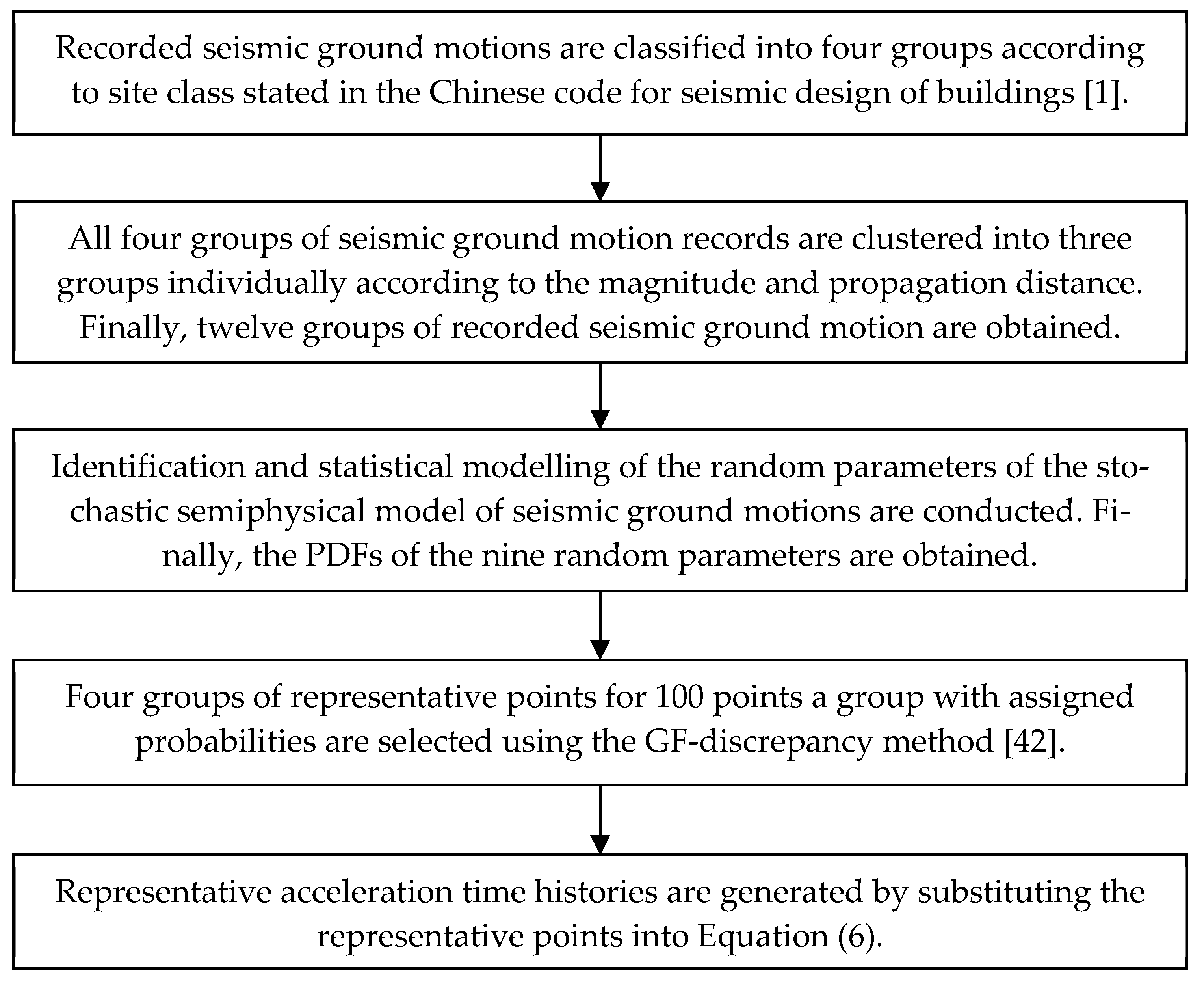
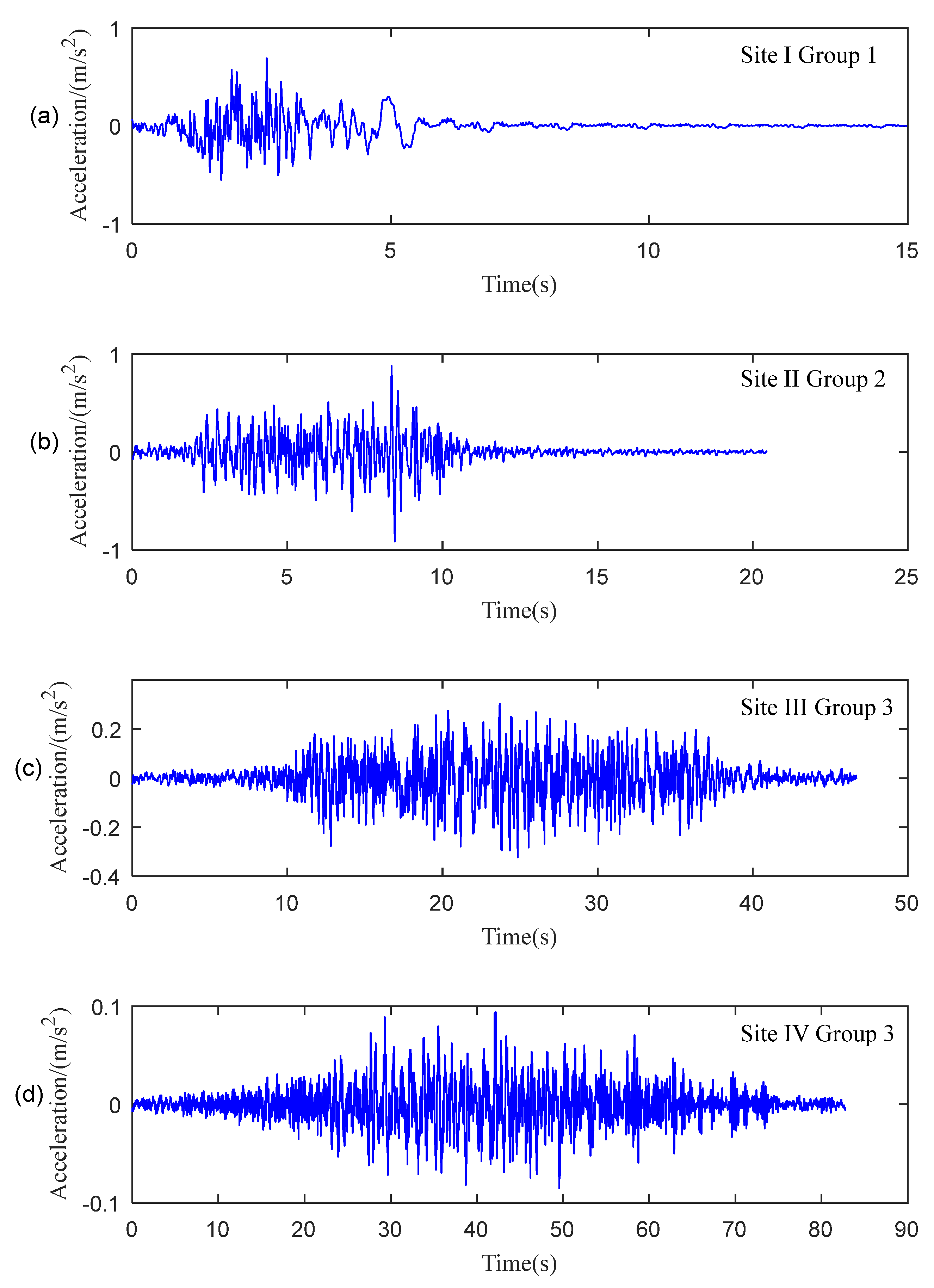
2.2. Simulation of Seismic Ground Motions

The superposition method of narrow-band wave groups was used for the simulation of seismic ground motions. In this method, the acceleration time history is [30]
a R ( t ) = j = 1 N F j ( t ) × A j × cos ( ω j t + Φ j ) × Δ ω
where A j is the amplitude with respect to ω j , computed by Equation (2); Φ j is the phase with respect to ω j , computed by Equation (3); and F j ( t ) is the amplitude envelope function [30] expressed as follows:
F j ( t ) = sin [ ( t R c j ) Δ ω ] t R c j
in which the group velocity c j [30] with respect to ω j is
c j = d ω d k ( ω ) | ω = ω j = a ω j + 1000 b + 0.1323 sin ( 3.78 ω j ) + c cos ( d ω j ) a + 0.5 cos ( 3.78 ω j ) c d sin ( d ω j )
Four hundred representative points with corresponding assigned probabilities were selected using the GF-discrepancy method based on the PDFs of the nine random parameters as presented in Table 2 [42]. The 400 representative points were divided into four groups by the same amount, i.e., group 1–group 4 corresponding to site I–site IV, respectively. Accordingly, representative time histories of seismic ground motion were synthesized by substituting the representative points into Equation (6). The process of the synthesis of the stochastic ground motions is shown in Figure 1.
Four typical simulated acceleration time histories, as shown in Figure 2, show big differences in peak ground acceleration (PGA) and duration. The mean response spectrum of the four groups of simulated seismic ground motions are shown in Figure 3. The PGAs of all the simulated seismic ground motions were normalized to 0.1 g before calculating their response spectrum for a consistent demand. The mean response spectrum of the four groups also show huge differences.

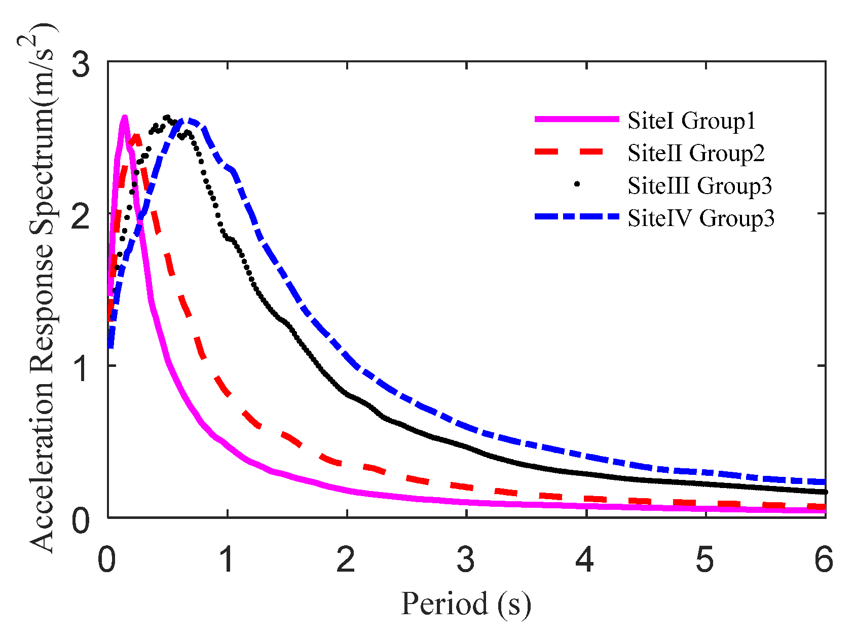
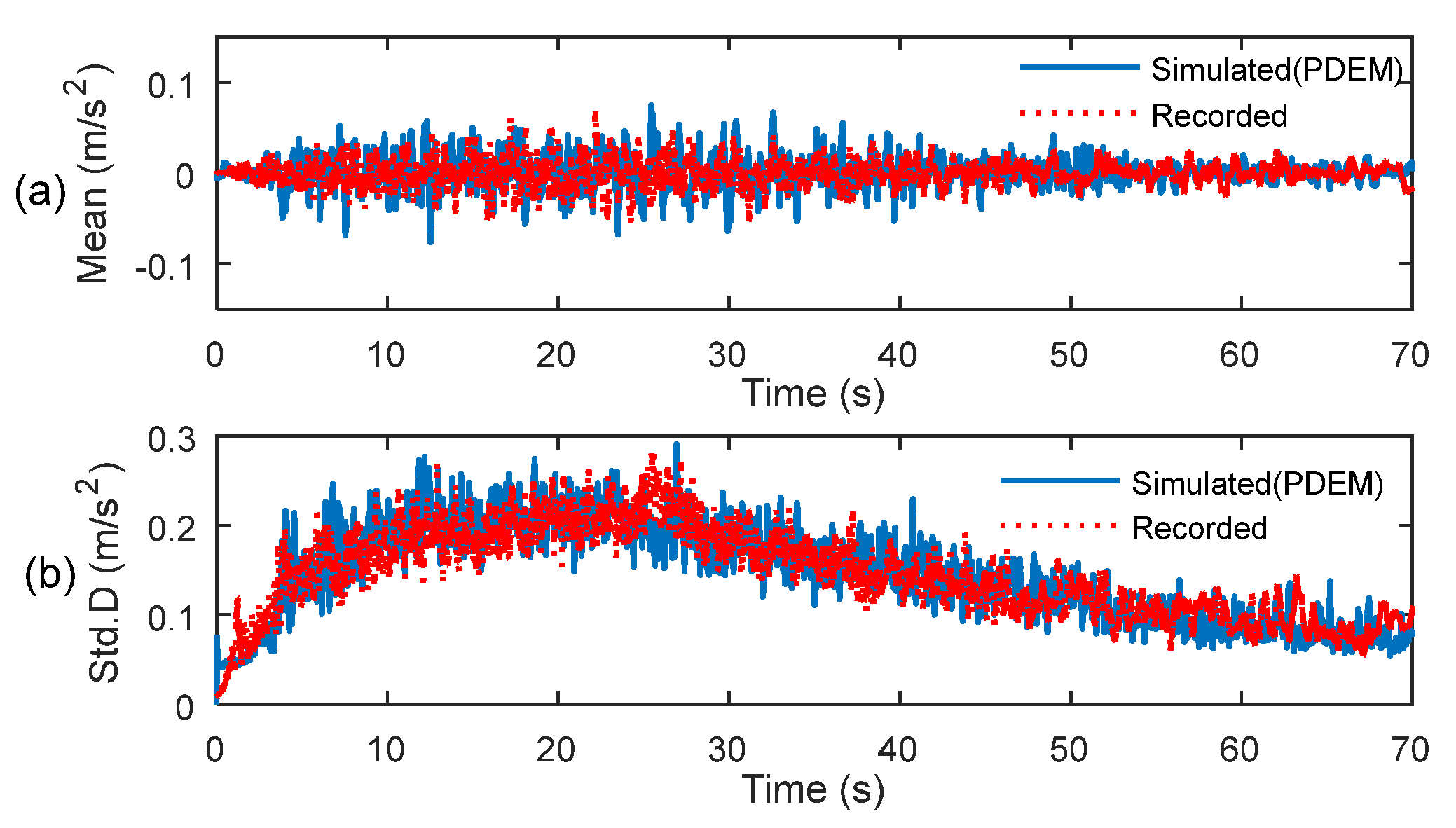
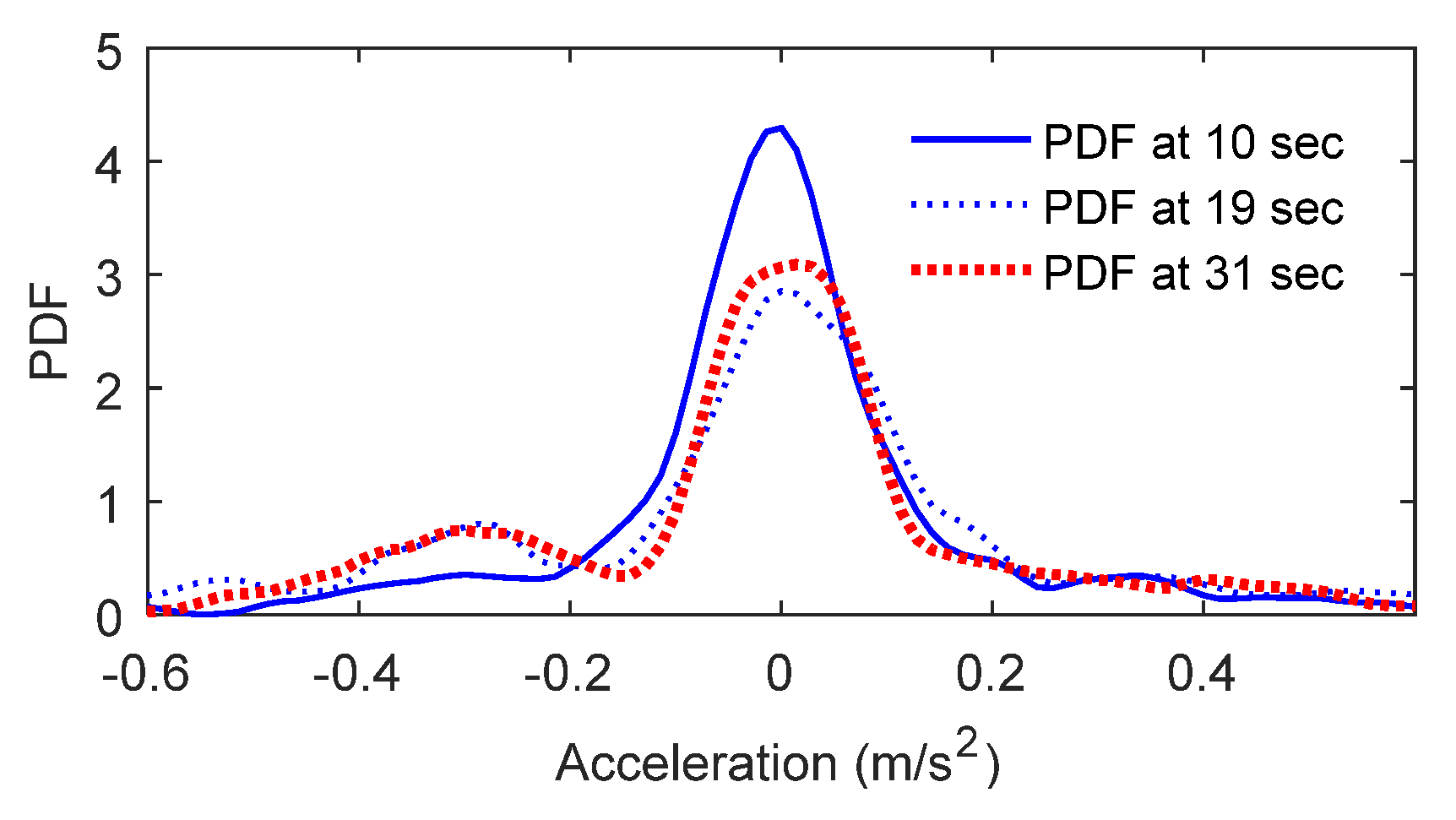
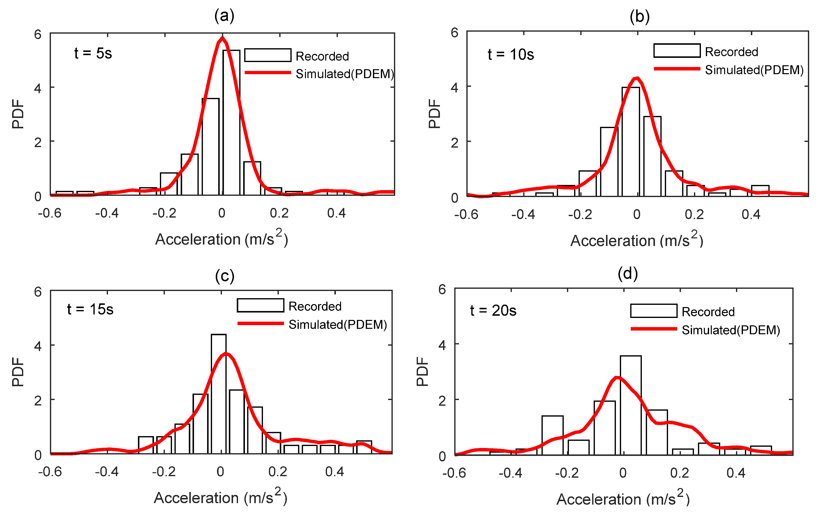
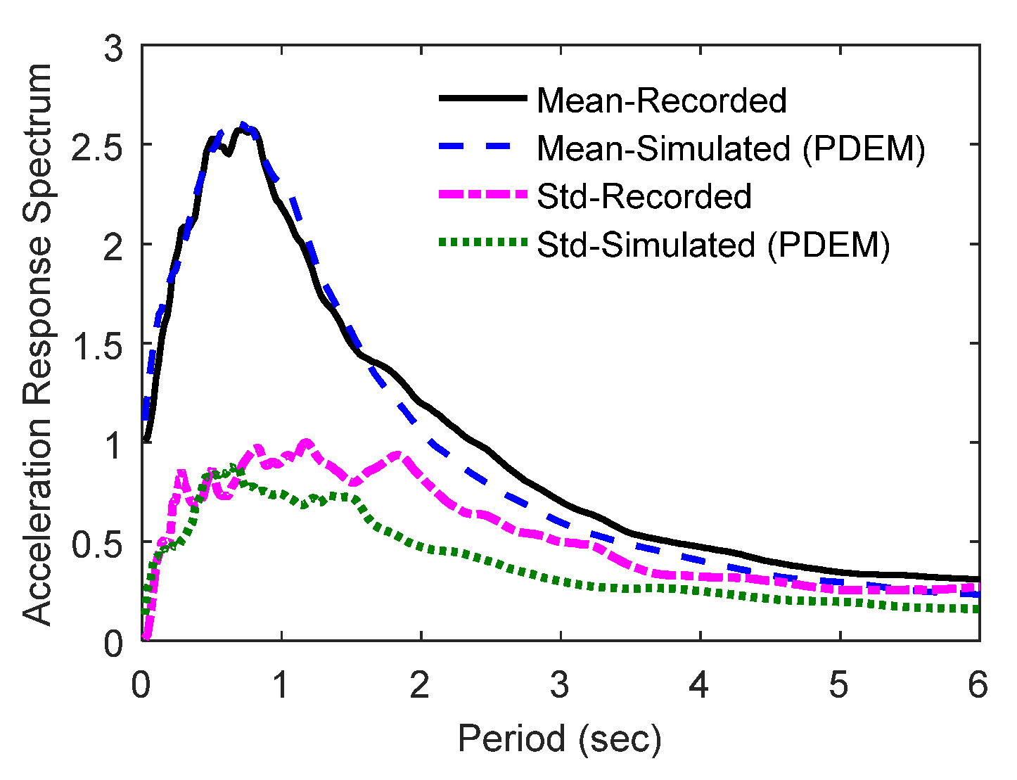
2.3. Validation of Simulated Seismic Ground Motions

Four groups of simulated seismic ground motions were validated using the PDEM. The simulated seismic ground motions of Site III group 3 are taken as an example in this section. Comparisons between the simulated and the recorded seismic ground motions in time history and response spectrum were carried out.
The PGAs of all the simulated and recorded seismic ground motions were normalized to 0.1 g for a consistent demand. Shown in Figure 4 is the comparison of mean and standard deviation between simulated and recorded seismic ground motions. The statistical moments of simulated seismic ground motions were obtained by the PDEM. The results show a good agreement between the simulated and recorded seismic ground motions in sense of the mean as well as the standard deviation. Figure 5 shows the probability density evolution of seismic ground motions calculated by the PDEM at different instants of time. It is seen that there exists a difference in the stage of strong shock due to significant fluctuation of seismic acceleration. Meanwhile, Figure 6 shows the statistical histogram of recorded seismic ground motions and the PDFs of simulated seismic ground motions calculated by the PDEM at typical instants: 5, 10, 15, and 20 s. It reveals that the probability densities of simulated seismic ground motions meet well with those of the recorded seismic ground motions. The comparisons of the response spectrum upon mean and standard deviation between the simulated and recorded seismic ground motions are shown in Figure 7. The figure reveals an almost agreement both upon the mean and the standard deviation.

3. Seismic Analysis Based on the Chinese Seismic Code

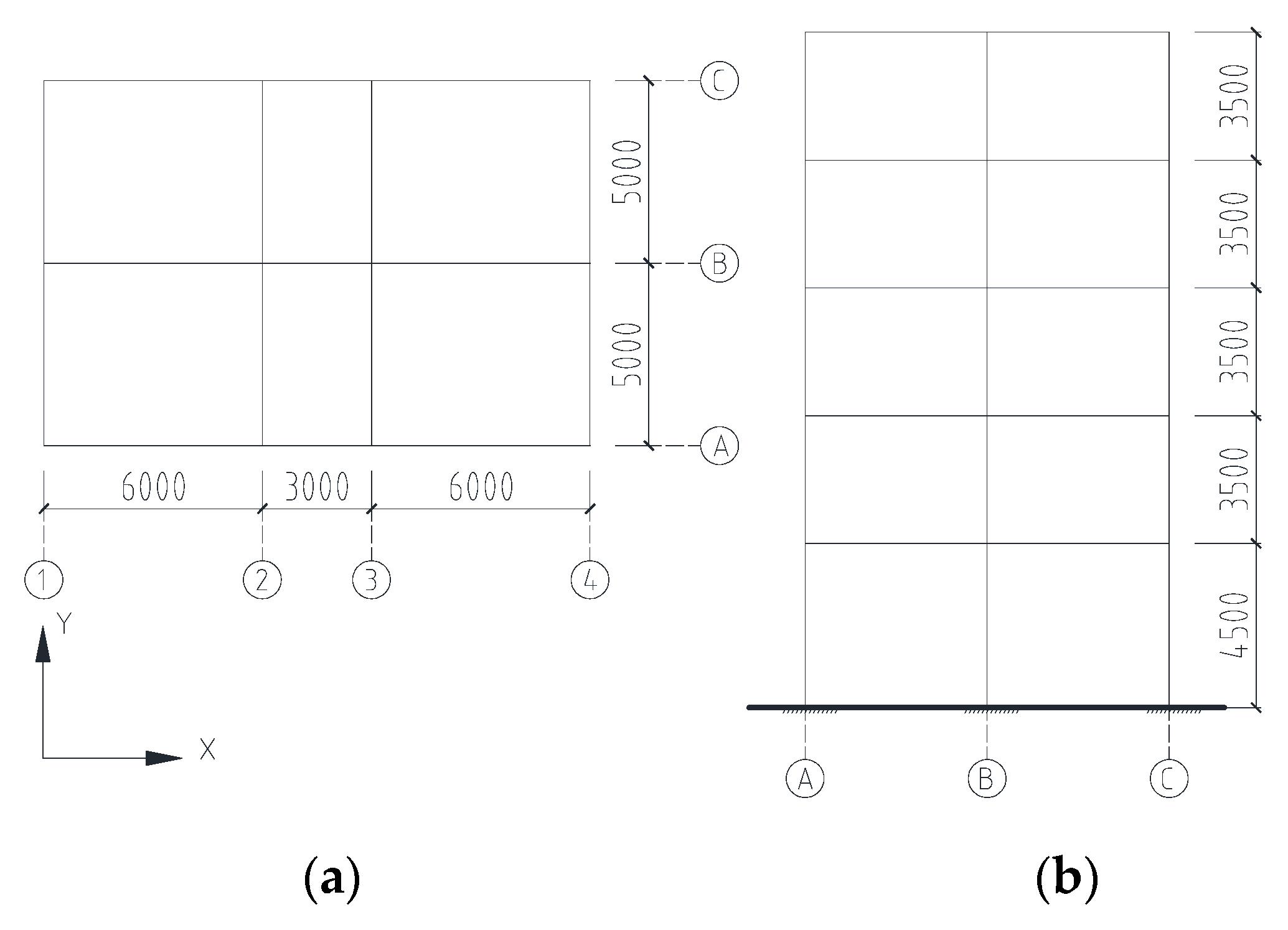
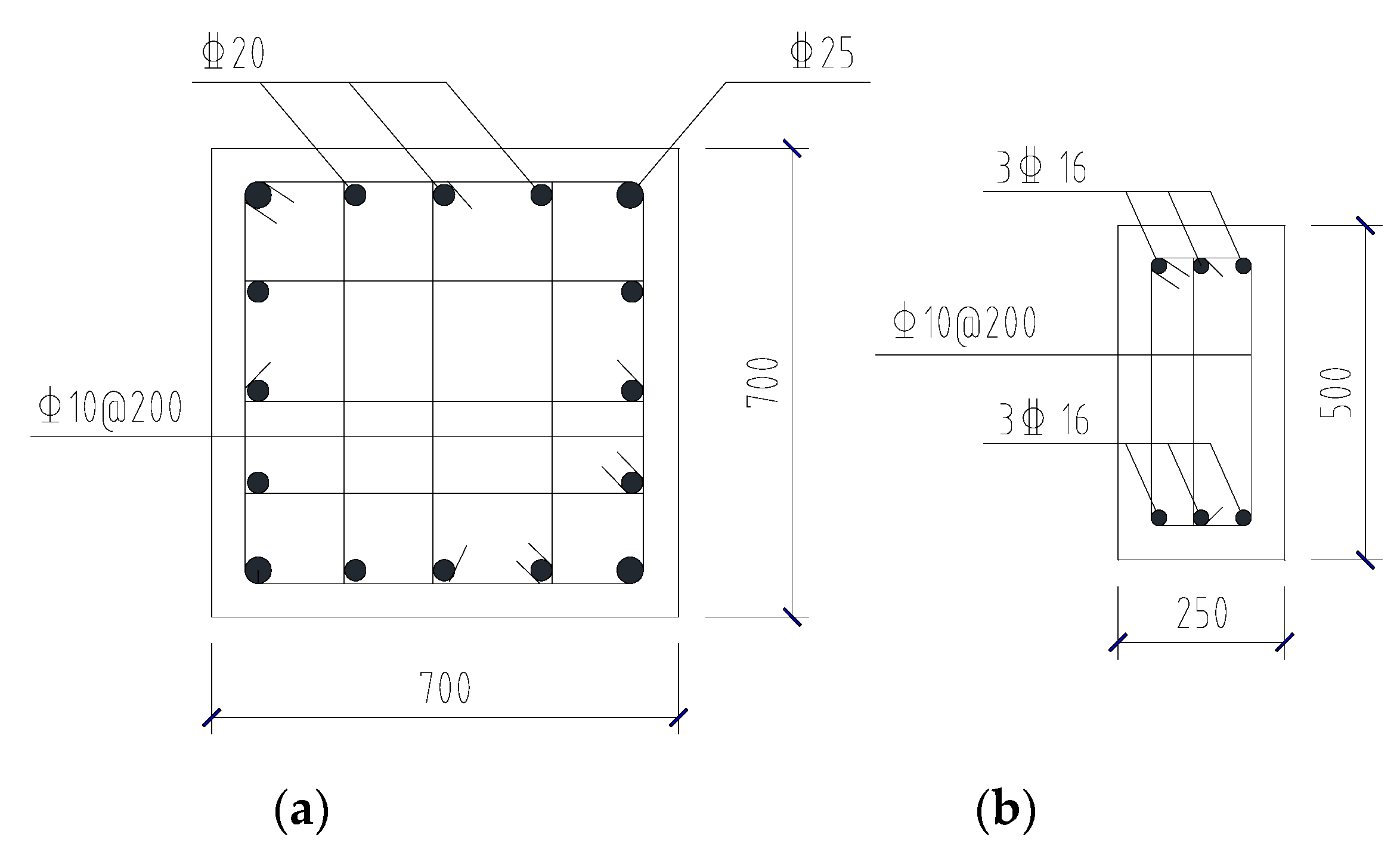
3.1. Introduction of a Reinforced Concrete Frame Structure

A five-story reinforced concrete frame structure is taken as an example to illustrate the proposed seismic checking method in this study. The plan and the elevation of the frame structure are shown in Figure 8. All the five floors shared the same plan, and all the beams, columns, and floor slabs of the frame structure shared the same sections, respectively. There were no holes in the floor. The thickness of the floor slabs was 100 mm. The reinforcement drawings of the beam and column were shown in Figure 9. According to the Chinese code for the seismic design of buildings (GB50011-2010) [1], the structure is located in the site with an eight-degree seismic fortification intensity, and the design basic acceleration of ground motion of the site is 0.2 g.
The 3D finite element model of the structure was first built using the Etabs software (Computers and Structures, Inc.; Berkeley, CA, USA); then it was transformed into an OpenSEES (University of California; San Francisco, CA, USA) model by a preprocessing software ETO (Xuewei Chen; Hong Kong, China) of the OpenSEES software. In the OpenSEES model, the Concrete 02 and Steel 02 materials were used. The parameters of the two materials are presented in Table 3. The fiber section and force-based beam–column element were used to model all the beams and columns. The Rayleigh damping with a 5% damping ratio was assigned to the model. The model was analyzed using the Newton algorithm. The first ten-order natural periods of the Etabs and OpenSEES models are presented in Table 4. It is indicated that the two models are similar to each other in mass and rigidity because the relative errors of the natural periods of the first ten orders are all less than 2%. In this study, the Etabs and OpenSEES models were used for the response spectrum method and dynamic analysis, respectively, for a convenient demand.

3.2. Seismic Checking Based on the Chinese Code for Seismic Design of Buildings

As presented in the Chinese code for the seismic design of buildings (GB50011-2010), the maximum value of the horizontal seismic influence coefficient of the frame structure in this study was 0.16 for frequent earthquakes and 0.9 for rare earthquakes. The design response spectrum of site I group 1, site II group 2, site III group 3, and site IV group 3 corresponding to the simulated seismic ground motions were used. The characteristic periods of the four spectra were 0.25, 0.4, 0.65, and 0.90, respectively, according to Chinese code for the seismic design of buildings (GB50011-2010). The thresholds of the elastic story drift angle and the elastoplastic story drift angle of the frame structure in this study were 1/550 and 1/50, respectively.
The max story drift angles of the frame structure excited by the design response spectrum were calculated using the response spectrum method for modal analysis. The elastoplastic story drift angle equals the product of the elastic story drift angle and the amplifying coefficient for the elastoplastic story drift angle of the Chinese code for the seismic design of buildings (GB50011-2010). The drift angles of the third story were maximum for all design response spectrum. As is presented in Table 5, the story drift angles calculated using the response spectrum method were much less than the thresholds. That is, the story drift angles of the structure satisfied the requirements of the code.

4. Dynamic Analysis and Evaluation of the Reliability of the Frame Structure Excited by Stochastic Ground Motions

The OpenSEES model was used for the dynamic analysis of the frame structure because it is much more time-saving than the Etabs model. The max seismic accelerations of ground motions used in the time-history analysis of the frame structure in this study were 0.7 m/s2 for frequent earthquakes and 4 m/s2 for rare earthquakes according to the Chinese code for the seismic design of buildings (GB50011-2010). Therefore, the four groups of stochastic simulated seismic ground motions in Section 2.2 were adjusted to 0.7 m/s2 for frequent earthquake analysis and 4 m/s2 for rare earthquake analysis. Four stochastic simulated ground motions were used for the dynamic analysis of the frame structure. Moreover, the PDEM was used for the analysis of the dynamic responses and reliability evaluation of the frame structure.

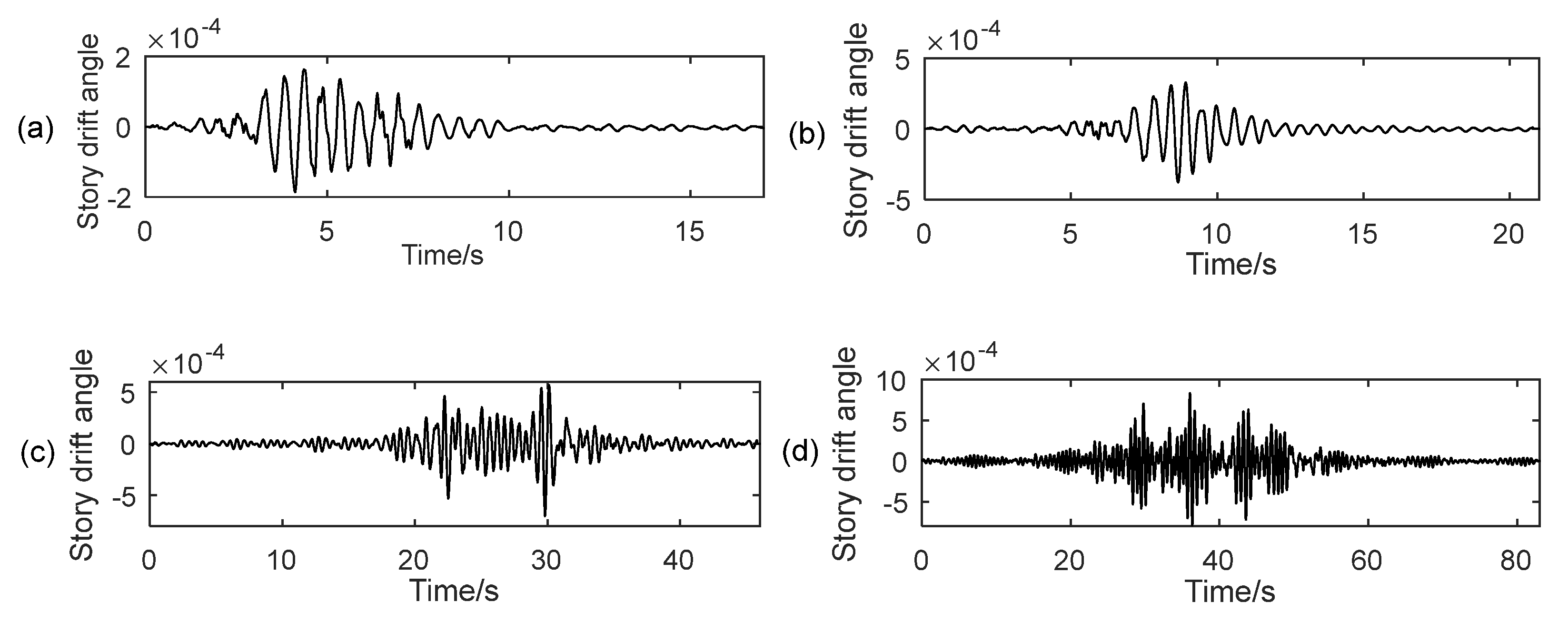
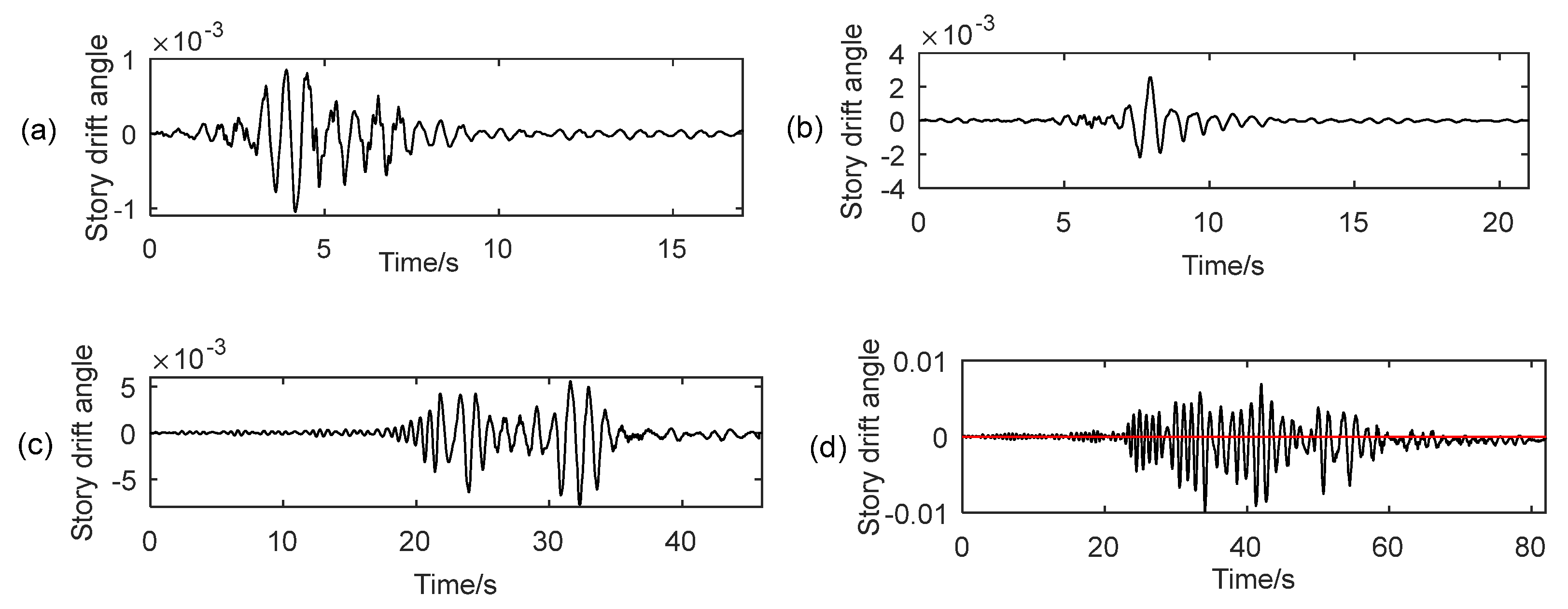
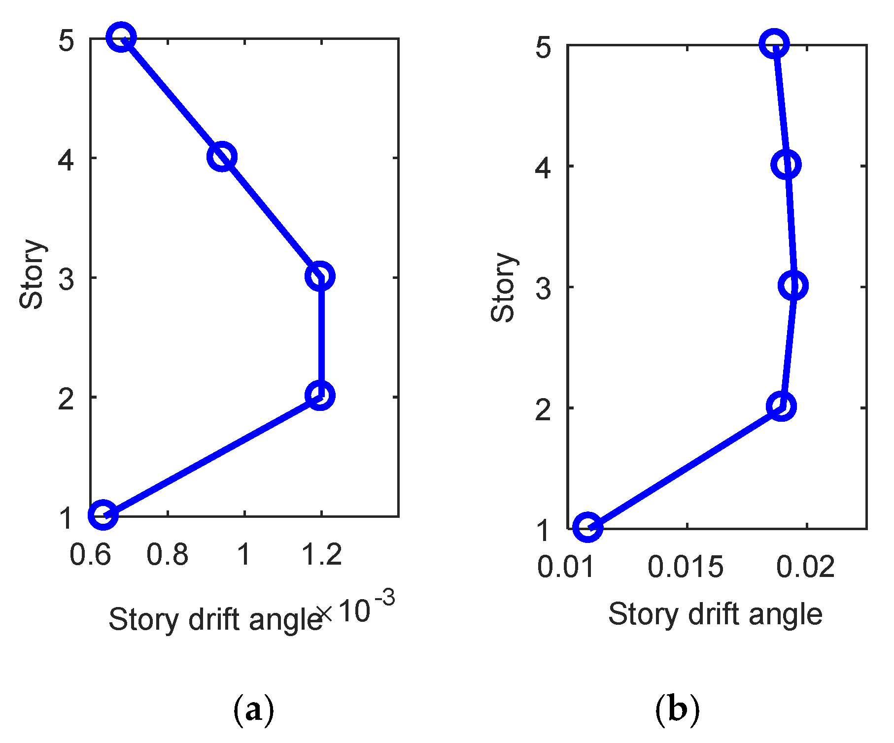
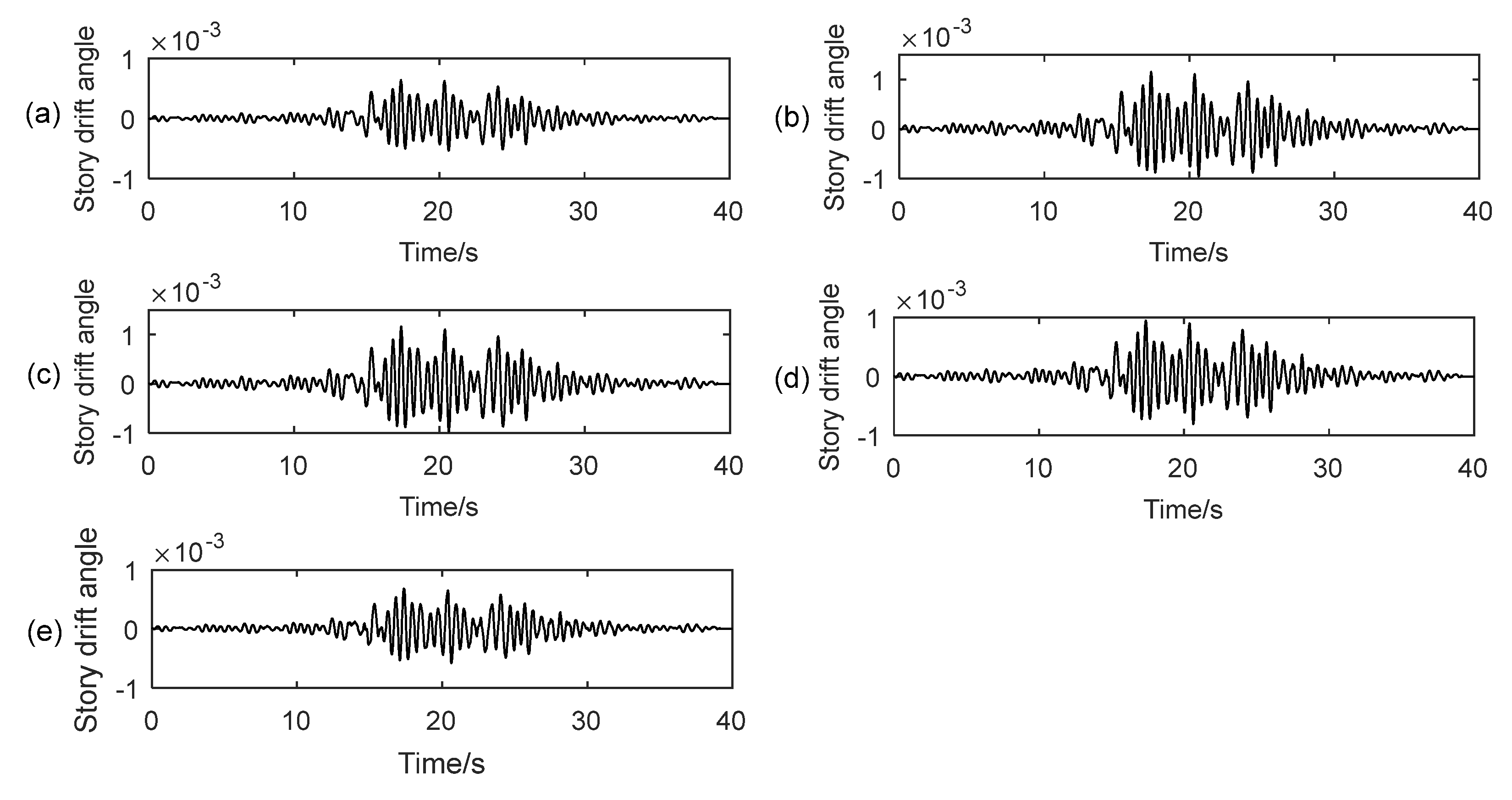
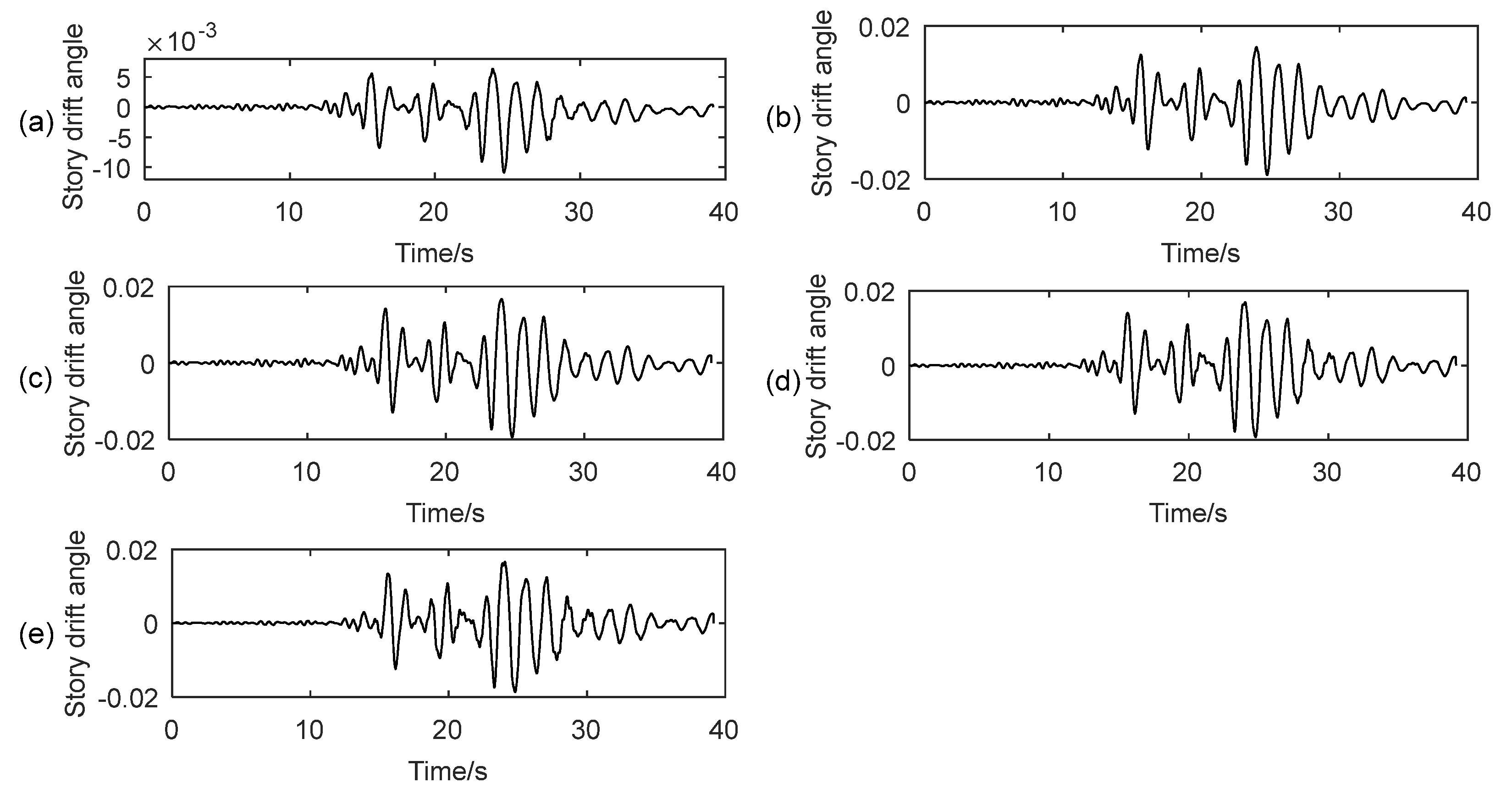
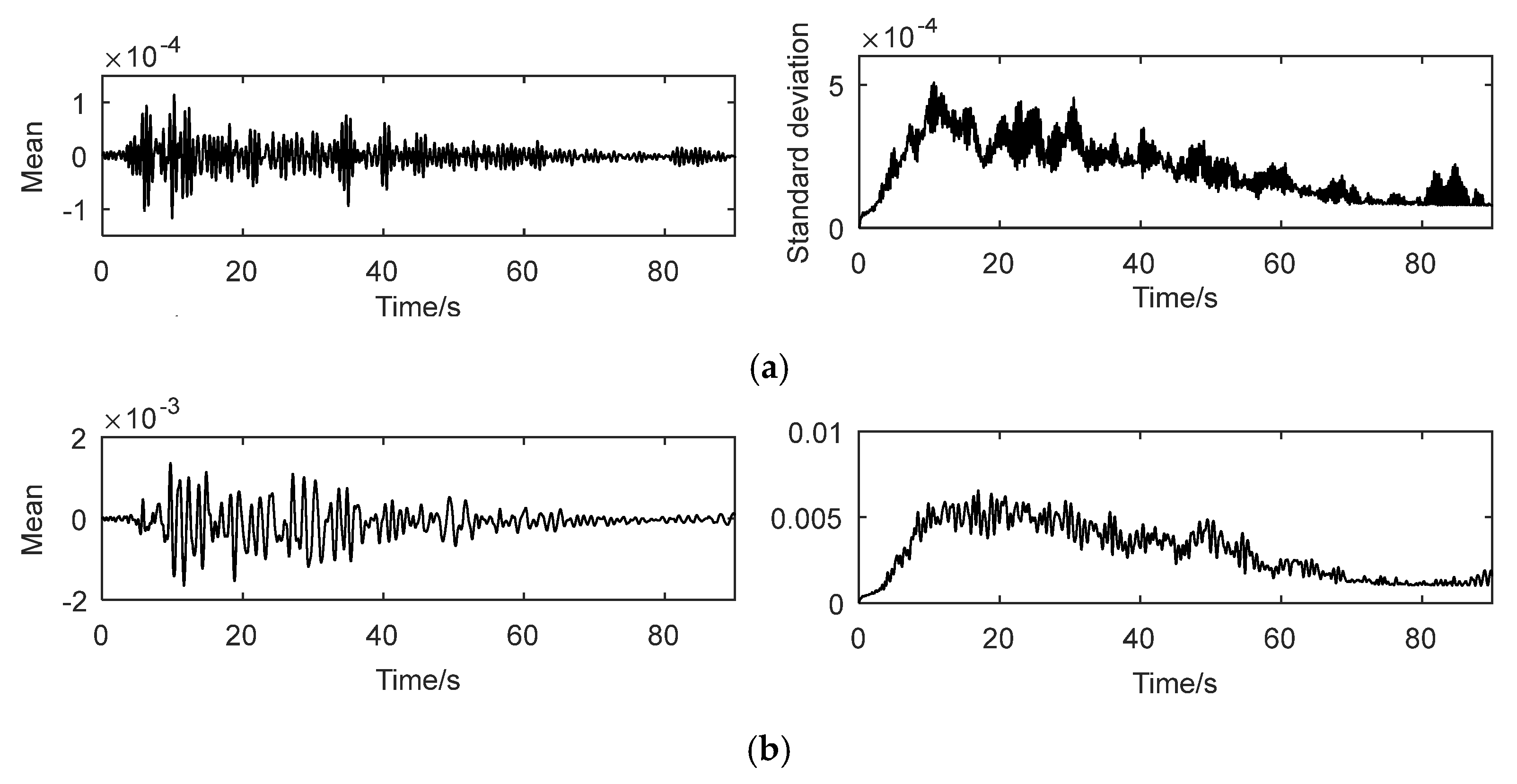
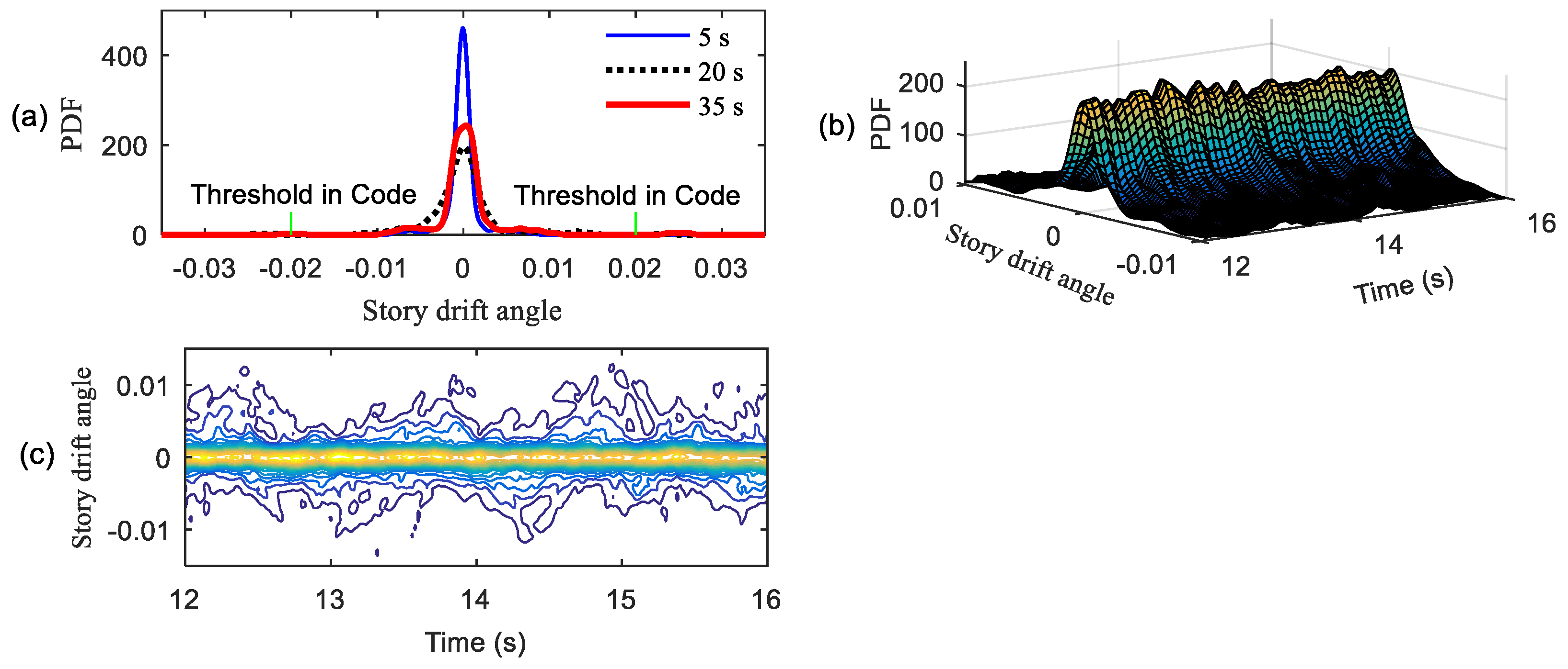
4.1. Dynamic Response of the Frame Structure

The typical story drift angle time histories of the bottom story for frequent and rare earthquakes are shown in Figure 10 and Figure 11, respectively. The story drift angle time histories of Figure 10 and Figure 11 are motivated by one acceleration time history with different PGAs, 0.7 m/s2 and 4 m/s2, respectively. Compared to Figure 10 and Figure 11, the story drift angle time histories of rare earthquakes are not only higher than those of the frequent earthquakes but also have different shapes than frequent earthquakes, which reveals that the dynamic performance of the frame structure changes when they were excited by rare earthquakes. As indicated in Figure 11d, it is seen that residual deformations exist (the red line in Figure 11d is a horizontal line). That is to say, the frame structure deforms plastically.
The max drift angles of all stories and story drift angle time histories of all the stories for frequent and rare earthquakes, excited by a certain acceleration time history with different PGAs, are shown in Figure 12, Figure 13 and Figure 14, respectively. These figures show that the story drift angles of the second and third stories are larger than those of the other stories for frequent earthquakes; the story drift angles from the second to fifth stories are larger than those of other stories for rare earthquakes.
The story drift angles of the third story under excitations of site IV group 3 stochastic simulated seismic ground motions are taken as an example. The mean and standard deviation time histories of the story drift angles are shown in Figure 15. The PDFs, PDF evolution surfaces, and contours of the PDF surface for frequent and rare earthquakes are shown in Figure 16 and Figure 17, respectively. As shown in Figure 16a and Figure 17a, the PDFs of the story drift angle at time instants, say, 5, 20, and 35s, show big differences. The thresholds of the story drift angles for frequent and rare earthquakes, i.e., 1/550 and 1/50, are also pictured in Figure 16a and Figure 17a, respectively. It is seen that the probability larger than the threshold is nonzero. Depicted in Figure 16b and Figure 17b is the time-varying process of the PDF, where the PDF varies with time just like mountains stretching into the distance. The contour of the PDF, shown in Figure 16c and Figure 17c, seems like water flowing in a river. They all show the evolution of the state that leads to probability flow in the time state space.

4.2. Dynamic Reliability Evaluation

The traditional synthesis methods of stochastic seismic ground motions, such as the spectral representation method, only describe the second-order statistic characteristics of seismic ground motions. In this case, the Monte Carlo method is used for the evaluation of reliability, which is very time-consuming. The stochastic semi-physical model of seismic ground motions describes the complete probabilistic information of ground motions including the higher moments and probabilistic density distributions, thus, the PDEM could be used for the evaluation of the reliability of structures.
To avoid the difficulty in dealing with the correlation among the component random events, Li et al. proposed a new approach for structural system reliability evaluation using the PDEM [43,44]. In this approach, the equivalent extreme-value event is introduced to make it possible to transform the computation of the probability of a compound random event into a one-dimensional integration of the PDF of the equivalent extreme value. In this section, the PDEM and the idea of the equivalent extreme-value event are used for the reliability evaluation of the frame structure.

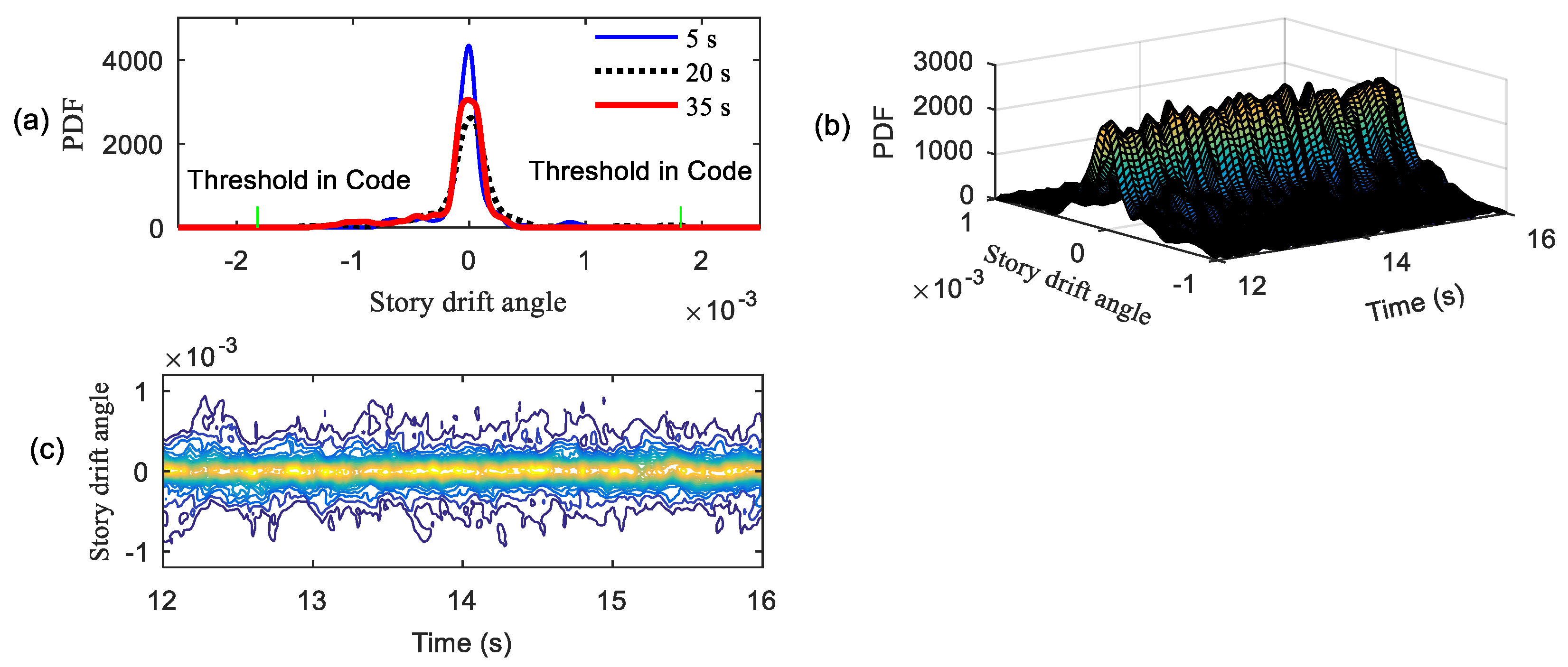
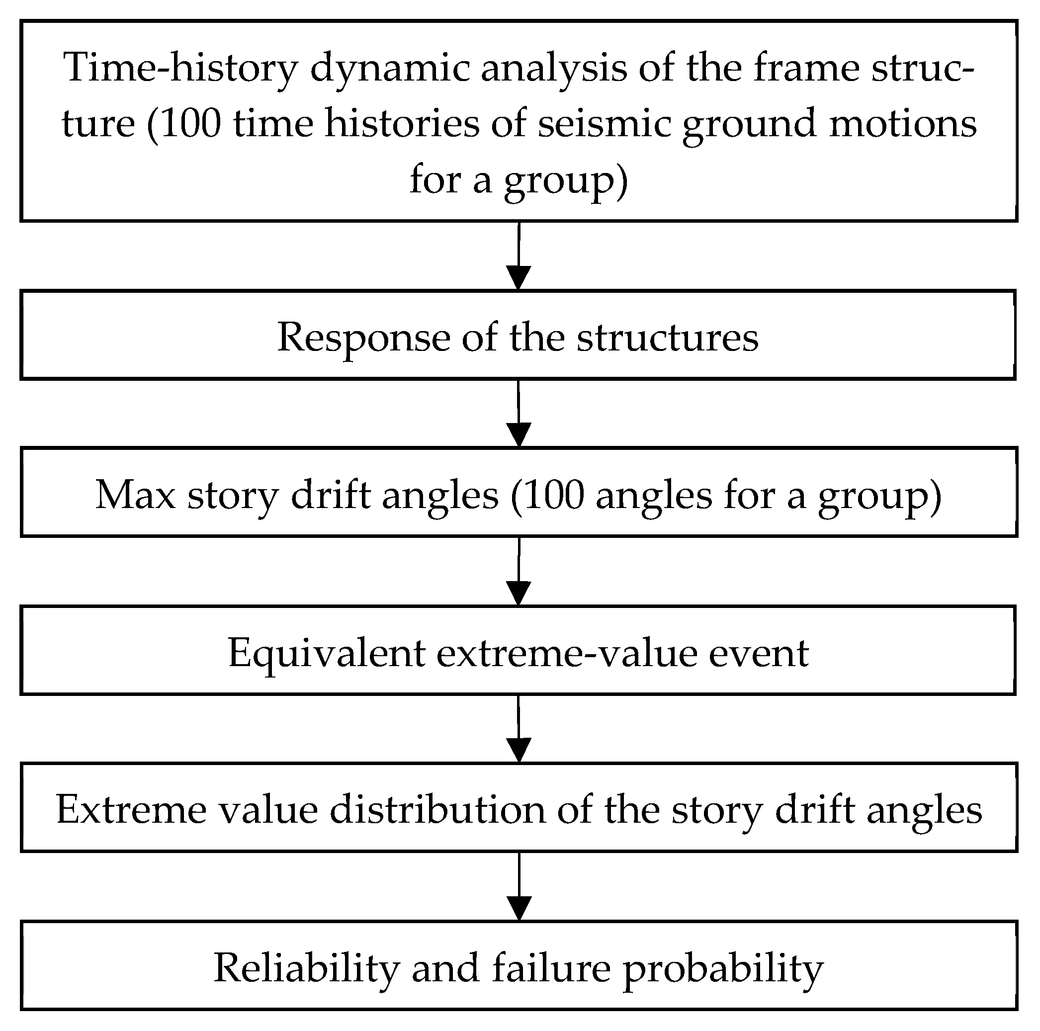
4.2.1. Evaluation of Reliability According to the Extreme Value Distribution

Denote the story drift angles of the structure as X i ( i = 1 , 2 , , m ) , where i is the story number. The equivalent extreme-value event is constructed as
ϕ ( Θ , t ) = X ˜ max ( t ) = max 1 i m { max 0 τ t | X i ( τ ) | }
where Θ is the random parameter vector of the whole dynamic system. In this study, Θ denotes the random parameters of the stochastic semi-physical model of seismic ground motions. The reliability of the structure is defined as
R ( t ) = Pr { i = 1 m [ | X i ( τ ) | b ] ,     0 τ t }
where Pr { } is the probability of the random event, b denotes the threshold of failure. According to the theorem of equivalent extreme-value events, the reliability is transformed into
R ( t ) = Pr { ϕ ( Θ , t ) b } = Pr { X ˜ max ( t ) b } = 0 b p X ˜ max ( x , t ) d x
where p X ˜ max ( x , t ) denotes the PDF of X ˜ max ( t ) . Equation (9) reveals that the reliability can be computed directly by a one-dimensional integration of the PDF p X ˜ max ( x , t ) . The PDF of X ˜ max ( t ) is computed by constructing a virtual stochastic process
Z ( τ ) = ψ [ ϕ ( Θ , t ) , τ ] = ϕ ( Θ , t ) cos ( 2 π T τ ) , τ c = T
By applying the PDEM, the reliability of the structure reads
R ( t ) = Pr { X ˜ max ( t ) b } = b p X ˜ max ( x , t ) d x = b p Z ( z , τ c ) d z

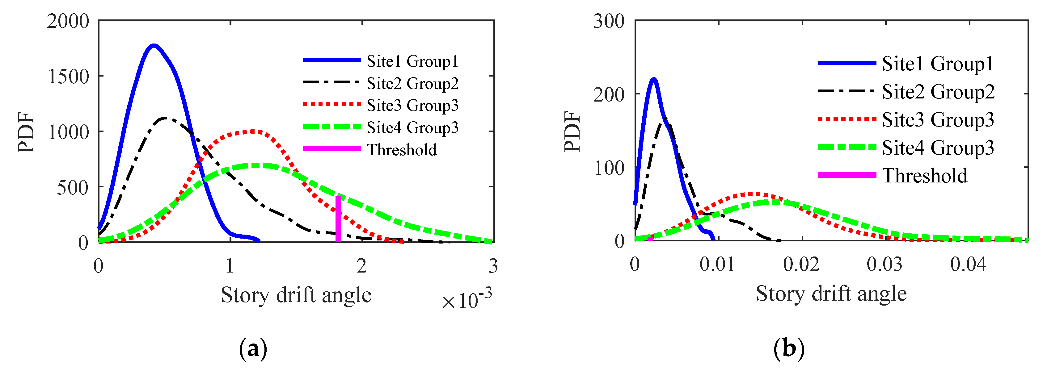
4.2.2. Reliabilities of the Frame Structure

The procedure of the reliability evaluation based on the PDEM and the idea of the extreme-value event are shown in Figure 18. Figure 19 pictures the PDF of the extreme values of story drift angles, which reveals a big difference for different groups of seismic ground motions. The failure thresholds are 1/550 and 1/50 for frequent and rare earthquakes, respectively, as mentioned in Section 2.2. Accordingly, the reliabilities and failure probabilities are presented in Table 6 and Table 7 for frequent and rare earthquakes, respectively.
It is seen that the failure probabilities of the frame structure under the ground motions of site IV group 3 reach up to 19.28% and 35.39% for frequent and rare earthquakes, respectively. There is also a larger failure probability of rare earthquakes for site III group 3. Compared with the results of seismic checking using the response spectrum method as presented in Table 5, it is concluded that the seismic checking method stated in the Chinese code needs to be improved for long-period seismic ground motions, especially for seismic ground motions with large PGAs.

5. Conclusions

The seismic checking method stated in the seismic code is incapable of evaluating the reliability of engineering structures and describing the strong stochasticity of seismic ground motions. In contrast, the seismic checking method proposed in this study includes the strong stochasticity of excitations by the stochastic semiphysical model of seismic ground motions. The stochastic semiphysical model of seismic ground motions can not only describe the strong stochasticity of earthquake ground motions but also generate artificial ground motions with different magnitudes, propagation distances, and shear velocities of sites. The simulated seismic ground motions show good agreement in spectral properties and time histories with the recorded ground motions. Compared with the widely used stochastic model of seismic ground motions, the stochastic semiphysical model of seismic ground motions has the advantage of including the complete probabilistic information of seismic ground motions. In conjunction with the PDEM, the dynamic reliability of structures could be easily evaluated through a one-dimensional integration of the PDF of the extreme value distribution of structural response.
A five-story reinforced concrete frame structure was analyzed using the response spectrum method and the proposed method, respectively. The responses of the structure analyzed by the response spectrum method are far less than the threshold stated in the seismic code. The results of the proposed method show that reliabilities are close to 100% when the structure is excited by seismic ground motions with small magnitudes and short propagation distances. However, as the magnitude and the propagation distance increase, the reliability of the structure decreases rapidly. Since the long-period components of seismic ground motions are amplified with the increase in the magnitude and propagation distance, it is indicated that the structure carries a higher risk of failure when the structure is excited by seismic ground motions with more long-period components. Comparing the results of the proposed method and the response spectrum method reveals that the strong stochasticity of seismic ground motions plays a significant role in the dynamic response of structures. Structures that satisfy the provisions stated in the seismic code may have a large failure probability in some special seismic conditions.
Though only one reinforced concrete frame structure is analyzed in this study, it is deduced that the proposed method is fit for more kinds of structures because the strong stochasticity is the key point. The stochastic semiphysical model of seismic ground motions based on the seismic checking method is also suitable for other kinds of structures, such as the steel structure or the reinforced concrete shear wall structure, and, more importantly, is suitable for the seismic checking of structures excited by long-period seismic ground motions in highly seismic areas.
For complex high-rise buildings, the proposed method will be much more time-consuming since multiple time-history analyses should be carried out. Nevertheless, the proposed method is still more effective than the Monte Carlo method. In future study, more recorded seismic ground motions are needed to increase the accuracy of simulated seismic ground motions, and the time-history analysis of structures should be improved for greater efficiency.

Author Contributions

Conceptualization, Y.D. and Y.X.; methodology, Y.D. and H.M.; software, H.M.; validation, H.M.; formal analysis, H.M.; investigation, Y.X. and H.M.; resources, Y.X. and H.M.; data curation, Y.X.; writing—original draft preparation, Y.D.; writing—review and editing, Y.X. and H.M.; visualization, Y.D.; supervision, Y.X. and H.M.; project administration, Y.D.; funding acquisition, Y.D. All authors have read and agreed to the published version of the manuscript.

Funding

This research was funded by the National Natural Science Foundation of China, grant number 52008339.

Institutional Review Board Statement

Not applicable.

Informed Consent Statement

Not applicable.

Data Availability Statement

Not applicable.

Acknowledgments

The support of the National Natural Science Foundation of China (Grant number 52008339) is highly appreciated. All the accelerograms used in this study are downloaded from the website of the Pacific earthquake engineering research center (PEER), http://ngawest2.berkeley.edu. The authors are also grateful to the PEER.

Conflicts of Interest

The authors declare no conflict of interest.

References

  1. Ministry of Housing and Urban-Rural Development. Code for Seismic Design of Buildings: GB 50011-2010; China Architecture and Building Press: Beijing, China, 2010.
  2. American Society of Civil Engineers. ASCE/SEI 7-05; Minimum Design Loads for Buildings and Other Structures; American Society of Civil Engineers: Reston, VA, USA, 2010. [Google Scholar]
  3. CEN. EN 1998-1. Eurocode 8, Design of Structures For Earthquake Resistance—Part 1: General Rules, Seismic Actions and Rules for Building; Comite Europeen de Normalisation (CEN): Brussels, Belgium, 2004. [Google Scholar]
  4. Ministry of Land, Infrastructure, Transport and Tourism. The Building Standard Law of Japan; Ministry of Land, Infrastructure, Transport and Tourism: Tokyo, Japan, 2001.
  5. Priestley, M.B. Evolutionary spectra and non-stationary processes. J. R. Stat. Soc. Ser. B 1965, 27, 204–229. [Google Scholar] [CrossRef]
  6. Liu, S.C. Evolutionary power spectral density of strong-motion earthquakes. Bull. Seismol. Soc. Am. 1970, 60, 891–900. [Google Scholar] [CrossRef]
  7. Lin, Y.K.; Yong, Y. Evolutionary Kanai-Tajimi earthquake models. J. Eng. Mech. 1987, 113, 1119–1137. [Google Scholar] [CrossRef]
  8. Liang, J.; Chaudhuri, S.R.; Shinozuka, M. Simulation of nonstationary stochastic processes by spectral representation. J. Eng. Mech. 2007, 133, 616–627. [Google Scholar] [CrossRef]
  9. Rezaeian, S.; Zhong, P.; Hartzell, S.; Zareian, F. Validation of simulated earthquake ground motions based on evolution of intensity and frequency content. Bull. Seismol. Soc. Am. 2015, 105, 3036–3049. [Google Scholar] [CrossRef]
  10. Karimzadeh, S. Seismological and engineering demand misfits for evaluating simulated ground motion records. Appl. Sci. 2019, 9, 4497. [Google Scholar] [CrossRef] [Green Version]
  11. Boore, D.M. Stochastic simulation of high-frequency ground motions based on seismological models of the radiated spectra. Bull. Seismol. Soc. Am. 1983, 73, 1865–1894. [Google Scholar]
  12. Boore, D.M. Simulation of ground motion using the stochastic method. Pure Appl. Geophys. 2003, 160, 635–676. [Google Scholar] [CrossRef] [Green Version]
  13. Shinozuka, M. Simulation of multivariate and multidimensional random processes. J. Acoust. Soc. Am. 1971, 49, 357–368. [Google Scholar] [CrossRef]
  14. Shinozuka, M.; Deodatis, G. Simulation of stochastic processes by spectral representation. Appl. Mech. Rev. 1991, 44, 191–204. [Google Scholar] [CrossRef]
  15. Liu, Z.; Liu, W.; Peng, Y. Random function based spectral representation of stationary and non-stationary stochastic processes. Probabilistic Eng. Mech. 2016, 45, 115–126. [Google Scholar] [CrossRef]
  16. Sarkar, K.; Gupta, V.K.; George, R.C. Wavelet-based generation of spatially correlated accelerograms. Soil Dyn. Earthq. Eng. 2016, 87, 116–124. [Google Scholar] [CrossRef]
  17. Chen, J.; Kong, F.; Peng, Y. A stochastic harmonic function representation for non-stationary stochastic processes. Mech. Syst. Signal Process. 2017, 96, 31–44. [Google Scholar] [CrossRef]
  18. Quinay, P.E.B.; Ichimura, T. An improved fault-to-site analysis tool towards fully HPC-enhanced physics-based urban area response estimation. J. Earthq. Tsunami 2016, 10, 1640018. [Google Scholar] [CrossRef]
  19. Amin, M.; Ang, A.H.S. Nonstationary stochastic models of earthquake motions. J. Eng. Mech. Div. 1968, 94, 559–584. [Google Scholar] [CrossRef]
  20. Fatemi, A.A.; Bagheri, A.; Amiri, G.G.; Ghafory-ashtiany, M. Generation of uniform hazard earthquake accelerograms and near-field ground motions. J. Earthq. Tsunami 2012, 6, 1250013. [Google Scholar] [CrossRef]
  21. Li, C.; Li, H.; Hao, H.; Bi, K.; Tian, L. Simulation of multi-support depth-varying earthquake ground motions within heterogeneous onshore and offshore sites. Earthq. Eng. Eng. Vib. 2018, 17, 475–490. [Google Scholar] [CrossRef]
  22. Rezaeian, S.; Der Kiureghian, A. A stochastic ground motion model with separable temporal and spectral nonstationarities. Earthq. Eng. Struct. Dyn. 2008, 37, 1565–1584. [Google Scholar] [CrossRef]
  23. Xu, J.; Zhang, W.; Sun, R. Efficient reliability assessment of structural dynamic systems with unequal weighted quasi-Monte Carlo simulation. Comput. Struct. 2016, 175, 37–51. [Google Scholar] [CrossRef]
  24. Shayanfar, M.A.; Barkhordari, M.A.; Roudak, M.A. An efficient reliability algorithm for locating design point using the combination of importance sampling concepts and response surface method. Commun. Nonlinear Sci. Numer. Simul. 2017, 47, 223–237. [Google Scholar] [CrossRef]
  25. Shayanfar, M.A.; Barkhordari, M.A.; Barkhori, M.; Barkhori, M. An adaptive directional importance sampling method for structural reliability analysis. Struct. Saf. 2018, 70, 14–20. [Google Scholar] [CrossRef]
  26. Jing, Z.; Chen, J.; Li, X. RBF-GA: An adaptive radial basis function metamodeling with genetic algorithm for structural reliability analysis. Reliab. Eng. Syst. Saf. 2019, 189, 42–57. [Google Scholar] [CrossRef]
  27. An, Z.; Li, J. Research on random function model of strong ground motion (Ⅰ): Model constructing. Earthq. Eng. Eng. Vib. 2009, 29, 36–45. [Google Scholar]
  28. An, Z.; Li, J. Research on random function model of strong ground motion (II): Parametric statistic and model certification. Earthq. Eng. Eng. Vib. 2009, 29, 40–47. [Google Scholar]
  29. Wang, D.; Li, J. Physical random function model of ground motions for engineering purposes. Sci. Sin. Technol. 2011, 54, 175–182. [Google Scholar] [CrossRef]
  30. Ding, Y.; Peng, Y.; Li, J. A stochastic semi-physical model of seismic ground motions in time domain. J. Earthq. Tsunami 2018, 12, 1850006. [Google Scholar] [CrossRef]
  31. Song, M. Studying Random Function Model of Seismic Ground Motion for Engineering Purposes. Master’s Thesis, Tongji University, Shanghai, China, June 2013. [Google Scholar]
  32. Ding, Y.; Peng, Y.; Li, J. Cluster analysis of earthquake ground-motion records and characteristic period of seismic response spectrum. J. Earthq. Eng. 2020, 24, 1012–1033. [Google Scholar] [CrossRef]
  33. Ding, Y.; Li, J. Parameters identification and statistical modelling of physical stochastic model of seismic ground motion for engineering purposes. Sci. Sin. Technol. 2018, 48, 1422–1432. [Google Scholar] [CrossRef]
  34. Li, J.; Chen, J.B. The principle of preservation of probability and the generalized density evolution equation. Struct. Saf. 2008, 30, 65–77. [Google Scholar] [CrossRef]
  35. Li, J. Probability density evolution equations: History, development and applications. In Proceedings of the 9th International Conference on Structural Safety and Reliability (ICOSSAR2009), Osaka, Japan, 12–17 September 2009. [Google Scholar]
  36. Li, J. A PDEM-based perspective to engineering reliability: From structures to lifeline networks. Front. Struct. Civ. Eng. 2020, 14, 1056–1065. [Google Scholar] [CrossRef]
  37. Zhou, T.; Peng, Y. Reliability analysis using adaptive Polynomial-Chaos Kriging and probability density evolution method. Reliab. Eng. Syst. Saf. 2022, 220, 108283. [Google Scholar] [CrossRef]
  38. Trifunac, M.D. Response envelope spectrum and interpretation of strong earthquake ground motion. Bull. Seismol. Soc. Am. 1971, 61, 343–356. [Google Scholar] [CrossRef]
  39. Liao, Z. Introduction to Wave Motion Theories in Engineering, 2nd ed.; Science Press: Beijing, China, 2002; pp. 23–25. [Google Scholar]
  40. Chen, J.; Li, J. A note on the principle of preservation of probability and probability density evolution equation. Probab. Eng. Mech. 2009, 24, 51–59. [Google Scholar] [CrossRef]
  41. Li, J.; Chen, J. Advances in the research on probability density evolution equations of stochastic dynamical systems. Adv. Mech. 2010, 40, 170–188. [Google Scholar]
  42. Chen, J.; Yang, J.; Li, J. A GF-discrepancy for point selection in stochastic seismic response analysis of structures with uncertain parameters. Struct. Saf. 2016, 59, 20–31. [Google Scholar] [CrossRef]
  43. Chen, J.; Li, J. The extreme value distribution and dynamic reliability analysis of nonlinear structures with uncertain parameters. Struct. Saf. 2007, 29, 77–93. [Google Scholar] [CrossRef]
  44. Li, J.; Chen, J.; Fan, W. The equivalent extreme-value event and evaluation of the structural system reliability. Struct. Saf. 2007, 29, 112–131. [Google Scholar] [CrossRef]
Figure 1. Synthesis of stochastic seismic ground motions.
Buildings 12 00488 g001
Figure 2. Typical simulated seismic ground motions. (a) Site I Group 1; (b) Site II Group 2; (c) Site III, Group 3; (d) Site IV Group 3.
Buildings 12 00488 g002
Figure 3. Mean acceleration response spectrum for different groups of simulated seismic ground motions.
Buildings 12 00488 g003
Figure 4. Comparison of simulated and recorded seismic ground motions. (a) mean; (b) standard deviation.
Buildings 12 00488 g004
Figure 5. Evolution of probability density at different time instants.
Buildings 12 00488 g005
Figure 6. Comparison between the statistical histogram of recorded seismic ground motions and PDF of simulated seismic ground motions calculated by PDEM at typical instants. (a) 5 s; (b) 10 s; (c) 15 s; (d) 20 s.
Buildings 12 00488 g006
Figure 7. Comparisons of the mean and standard deviation of response spectrum of simulated seismic ground motions and those of recorded seismic ground motions.
Buildings 12 00488 g007
Figure 8. The plan and elevation of the structure (unit: mm). (a) plan; (b) elevation.
Buildings 12 00488 g008
Figure 9. The reinforcement drawings. (a) beam; (b) column.
Buildings 12 00488 g009
Figure 10. Story drift angle time histories of the bottom story of the frame structure under typical seismic ground motions (frequent earthquakes): (a) site I group 1; (b) site II group 2; (c) site III group 3; (d) site IV group 3.
Buildings 12 00488 g010
Figure 11. Story drift angle time histories of the bottom story of the frame structure under typical seismic ground motions (rare earthquakes): (a) site I group 1; (b) site II group 2; (c) site III group 3; (d) site IV group 3.
Buildings 12 00488 g011
Figure 12. Max story drift angles of each story of the frame structure under a certain stochastic simulated seismic ground motion: (a) frequent earthquakes; (b) rare earthquakes.
Buildings 12 00488 g012
Figure 13. Story drift time histories of different stories under a certain seismic ground motion (frequent earthquakes): (a) first story; (b) second story; (c) third story; (d) fourth story; (e) fifth story.
Buildings 12 00488 g013
Figure 14. Story drift angle time histories of different stories under a certain seismic ground motion (rare earthquake): (a) first story; (b) second story; (c) third story; (d) fourth story; (e) fifth story.
Buildings 12 00488 g014
Figure 15. Mean value and standard deviation time histories of story drift angles of the third story excited by stochastic simulated seismic ground motions of site IV group 3: (a) frequent earthquakes and (b) rare earthquakes.
Buildings 12 00488 g015
Figure 16. Story drift angles of the third story excited by stochastic simulated seismic ground motions of site IV group 3 (frequent earthquake): (a) probability distribution at certain time instants; (b) PDF evolution surface; (c) contour of the PDF surface.
Buildings 12 00488 g016
Figure 17. Story drift angles of the third story excited by stochastic simulated seismic ground motions of site IV group 3 (rare earthquake): (a) probability distribution at certain time instants; (b) PDF evolution surface; (c) contour of the PDF surface.
Buildings 12 00488 g017
Figure 18. Computation of reliability based on the PDEM and the idea of the extreme-value event.
Buildings 12 00488 g018
Figure 19. Extreme value distributions of story drift angle under different groups of stochastic simulated seismic ground motions: (a) frequent earthquake (b) rare earthquake.
Buildings 12 00488 g019
Table 1. Random parameters of the stochastic semiphysical model of seismic ground motions.
Random ParametersMeaning
A 0 amplitude parameter of the source
τ Brune source parameter describing the decay process of the fault rupture
ξ g equivalent damping ratio of the site
ω g equivalent predominate circular frequency of the site
R epicentral distance
a , b , c , d empirical parameters of the propagation path
Table 2. Parameters of PDFs of random parameters of the stochastic semi-physical model of seismic ground motions.
Random ParametersDistribution FunctionParameters of the PDFClustered Groups
Group 1Group 2Group 3
A 0 Lognormal μ −1.4872−1.1090−0.7155
σ 0.86390.79060.6944
τ Lognormal μ −2.7141−2.2853−1.4397
σ 1.42571.95701.8048
a Lognormal μ −0.3423−0.2505−0.3373
σ 0.38710.44000.3463
b Lognormal μ 0.20490.26790.0585
σ 0.87440.87660.4893
c Lognormal μ −1.1262−1.1613−1.9142
σ 1.15151.24871.4716
d Lognormal μ −1.0040−1.0311−1.8026
σ 0.93491.14731.2376
R Lognormal μ 2.95883.66255.3250
σ 1.1731.0100.2619
Random ParametersDistribution FunctionParameters of the PDFSite Class
IIIIIIIV
ξ g Gamma α 3.15573.99793.81133.3281
1 / β 0.12230.09380.09850.0924
ω g Lognormal μ 2.21072.39982.24172.0178
σ 1.31110.99860.82330.5058
Table 3. Materials and strengths.
MaterialYoung’s Modulus/MPaCompressive Strength/MPaTensile Strength/MPa
Concrete32,500313.22
Steel200,000400400
Table 4. Natural periods of the structure.
ModesNatural Periods
EtabsOpenSEESRelative Error
10.49590.49780.368%
20.47510.47070.926%
30.43710.44411.599%
40.32400.32380.039%
50.31090.30751.063%
60.22990.22980.044%
70.15030.14910.787%
80.14890.14900.042%
90.14850.14621.541%
100.13130.12941.466%
Table 5. Max story drift angles obtained by the response spectrum method.
Site and GroupSite I
Group 1
Site II
Group 2
Site III
Group 3
Site IV
Group 3
Limit of the Code
Frequent Earthquake1/19491/12381/10561/10561/550
Rare Earthquake1/1741/1101/941/941/50
Table 6. Reliability and failure probability for frequent earthquakes.
Site and GroupSite I
Group 1
Site II
Group 2
Site III
Group 3
Site IV
Group 3
Reliability100%97.79%95.13%80.72%
Failure Probability02.21%4.87%19.28%
Table 7. Reliability and failure probability for rare earthquakes.
Site and GroupSite I
Group 1
Site II
Group 2
Site III
Group 3
Site IV
Group 3
Reliability100%100%79.66%64.61%
Failure Probability0020.34%35.39%
Publisher’s Note: MDPI stays neutral with regard to jurisdictional claims in published maps and institutional affiliations.

