Study of an Integrated Control Method for Heating Substations Based on Prediction of Water-Supply Temperature and Indoor Temperature

Abstract

The refined control of heating substations is of great significance for on-demand heating provision and for the efficient operation of district heating systems (DHSs). This paper proposes an integrated control strategy for substations based on the prediction of the water-supply temperature and indoor temperature. Firstly, online sequential extreme learning machine (OS-ELM) is used to predict the water-supply temperature. Then, a linear prediction model is established to predict the indoor temperature. Finally, the integrated regulation strategy is established with the goal of minimizing operational costs, aiming at ensuring heating quality and meeting the limits of the flow rate and of the supply- and return-water temperatures. The heat-saving rate, power-saving rate and indoor-temperature satisfactory rate are introduced to evaluate the regulation effect of the proposed method. The field study results show that the performance index of operation executed with the regulation strategy proposed in this paper is 9.31%, 16.33% and 20.87% higher than that without our energy-saving regulation strategy respectively. The fluctuations in the water-supply pressure and differential pressure of the secondary network are significantly reduced, and the energy-saving effect is obvious.

1. Introduction

Heating systems account for about 21% of building energy consumption and are the key objects of low-carbon energy reforms [1]. The increasing pressure of the carbon-reduction issue represents a challenge for the heating sector in terms of achieving clean and efficient heating systems [2]. When aiming at ensuring users’ thermal comfort, to achieve on-demand heating provision, energy conservation and consumption reduction is an urgent problem. The operational optimization of heating systems has attracted a lot of attention, especially with respect to the optimization of economic performance. For example, aiming at minimizing operational costs, Gu et al. [3] proposed an optimization model based on mixed integer nonlinear programming considering the thermal inertia of district heating networks and buildings. The obtained results of a simulation of an actual heating system in Jilin Province showed high wind-power utilization with low operational costs. Fang et al. [4] used the genetic algorithm (GA) to optimize the water-supply temperature of a multi-heat-source branch heating network, with the goal of optimizing the total costs of fuel consumption and pump power consumption of the heating system. There are also studies on strategies for the multi-objective optimization of heating systems.

Research on the model predictive control of heating parameters such as water-supply temperature and return-water temperature is also gradually increasing. Lin et al. [5] developed a model predictive control system for district heating systems (DHSs) based on the cyber physical system. The system takes the minimization of pollutant-emission penalty costs and heating economic costs as the goal; it adds constraints such as operating load, pollutant emission and pipeline transportation capacity; and it uses the PSO algorithm to obtain the best multi-heat-source load-distribution parameters. After applying this regulation method, the consumption of natural gas was reduced by 31.2%, and the total heating cost was reduced by 2.6%. Conink et al. [6] proposed a model predictive control strategy using the grey-box control model, which considers the system energy-consumption cost and the user thermal-discomfort cost. The method was applied to a medium-sized office building, comparing heating days, thermal comfort, energy costs and primary energy consumption. The results show that the model predictive controller could make better use of the water-supply temperature and provide users with better thermal comfort. Compared with the rule-based control system, the heating cost was reduced by more than 30%. Benakopoulos et al. [7] proposed a low-temperature operational strategy for a thermostatic-valve radiator without preset functions for when the difference between the minimum water-supply temperature and radiator temperature is small. The operation of the system was analyzed through the thermal hydraulic model. The results showed that a lower water-supply temperature reduced the reflux temperature. Among the above research studies on model predictive control, most of them take the minimum heating economic cost as the goal and the allowable range of heating-system operational parameters as the constraint condition, and the control of the operation of the heating station is based on future interference, so as to meet the heat demand of users. Few studies have been conducted on a real-time optimization strategy considering the user indoor-temperature demand and thermal behavior.

With the development of Internet of Things (IoT) technology, the measurement of indoor temperature has been vigorously promoted in China’s DHSs in recent years. This particularly large data set provides conditions for research on the feedback control method and performance test of thermal power stations. Yuan et al. [8] studied the feedback prediction model based on indoor temperature to improve the operational efficiency of thermal power stations. This method uses the first-order linear steady-state model to deduce the relationship model between the water-supply temperature of the thermal station and the indoor and outdoor air temperatures. Considering the solar radiation and the uncertainty of the weather, in this model, the water-supply temperature is corrected every 10 min and applied to a thermal station. Dahlblom et al. [9] modified the water-supply temperature based on the actual indoor temperature on the basis of the feedforward control of the existing thermostatic-valve heating system. Such a control strategy could obtain a more constant indoor temperature and could be applied to buildings in southern Sweden. Liao et al. [10] simulated a boiler controller through experiments and simulations and applied the indoor-temperature feedback to the boiler controller to improve the performance of the heating system. The method was applied to an office building, and the results showed that the overheating phenomenon was greatly reduced. Sun et al. [11] proposed a dynamic control strategy based on online prediction and indoor-temperature measurements.

Song et al. [12] proposed an HA-GRU neural network to predict the indoor temperature of energy-saving buildings. The network can realize the fusion of a single influencing factor and multiple features. The simulation results showed that the prediction accuracy of the algorithm was 98.4%, and that it had good nonlinear-feature-extraction and -expression abilities. The indoor-temperature prediction results were used as feedback input to improve energy efficiency. Salo et al. [13] proposed a new model to control the indoor temperature by controlling the set temperature of the thermostatic radiator valve based on a prediction algorithm via a cloud platform considering the collected outdoor-temperature values and user feedback. The results showed that the indoor-temperature regulation with a single set point was more accurate.

The accurate prediction of the indoor temperature is very important for fine regulation. Li et al. [14] proposed an indoor-temperature predictive control method based on an Elman neural network multi-step predictive model for the predictive control of the indoor-temperature time delay in VAV air-conditioning systems. The experimental results showed that this method was conducive to improving the stability of the indoor-temperature control loop. Brandi et al. [15] proposed deep reinforcement learning to optimize the indoor-temperature control method in an integrated simulation environment. Shnayder [16] et al. established a building inverse-dynamic simulation model including indoor air temperatures for the feedforward control of heating systems. The model can evaluate the unmeasured indoor temperature in real time, and the lag of the heating cycle is considered in the process of control. Jian et al. [17] studied an optimization method of water-supply temperatures based on simulations according to the relationship among outdoor temperature, indoor temperature and water-supply temperature. By comparing the indoor temperature and optimized energy consumption, they showed that this method can appropriately reduce overheating and ensure that the indoor temperature is at the set point. Cano [18] predicted the short-term indoor temperature through a Bayesian neural network according to actual operational data to realize the real-time monitoring and management of a heating system. Aguilera et al. [19] proposed an indoor-temperature prediction method based on meteorological parameters which takes the average outdoor temperature, relative outdoor humidity, solar radiation and building attributes as input parameters and analyzes and simulates the data obtained from seven Danish family houses. The results showed that the accuracy of indoor-temperature prediction was 92%. The average outdoor temperature and personnel are important influencing parameters for predicting the indoor temperature, which provides a basis for the subsequent development of a simpler method for predicting the room temperature. Liu et al. [20] established an indoor-temperature prediction model based on the building equivalent heat capacity, determined the appropriate switching time and proposed a temperature- and time-sharing dynamic control method based on wireless indoor-temperature monitoring and a control system. Taking the DHS of a university teacher’s apartment as an example, the effectiveness of the method was verified.

The regulation of heating stations in DHSs is mostly feedforward control which considers outdoor meteorological parameters, historical operational parameters and indoor temperatures. In DHSs, the heat load changes with the outdoor temperature, solar radiation, occupant behavior and other factors. At present, the open-loop feedforward control mode considering the interference of outdoor meteorological parameters is mostly adopted in thermal power stations. With the development of IoT technology, the indoor-temperature acquisition technology of heat users has been widely used. In the operational regulation of heating stations of heating systems in the future, feedforward–feedback compound regulation should be realized aiming at the indoor thermal comfort of users. Secondly, the variations in the indoor temperature and the comprehensive outdoor air temperature are dynamic processes that change with time, and the heat load also changes. Therefore, it is particularly important to formulate a dynamic compound regulation strategy to provide on-demand heating via heating systems.

In order to improve the control effect of heating substations, this paper proposes an integrated strategy featuring the minimization of operational costs by combining water-supply-temperature and indoor-temperature predictions. The rest of the paper is organized as follows: Section 2 describes the establishing process of the method; Section 3 introduces the case study; results and discussion are presented in Section 4; Section 5 presents the main conclusions.

2. Materials and Methods

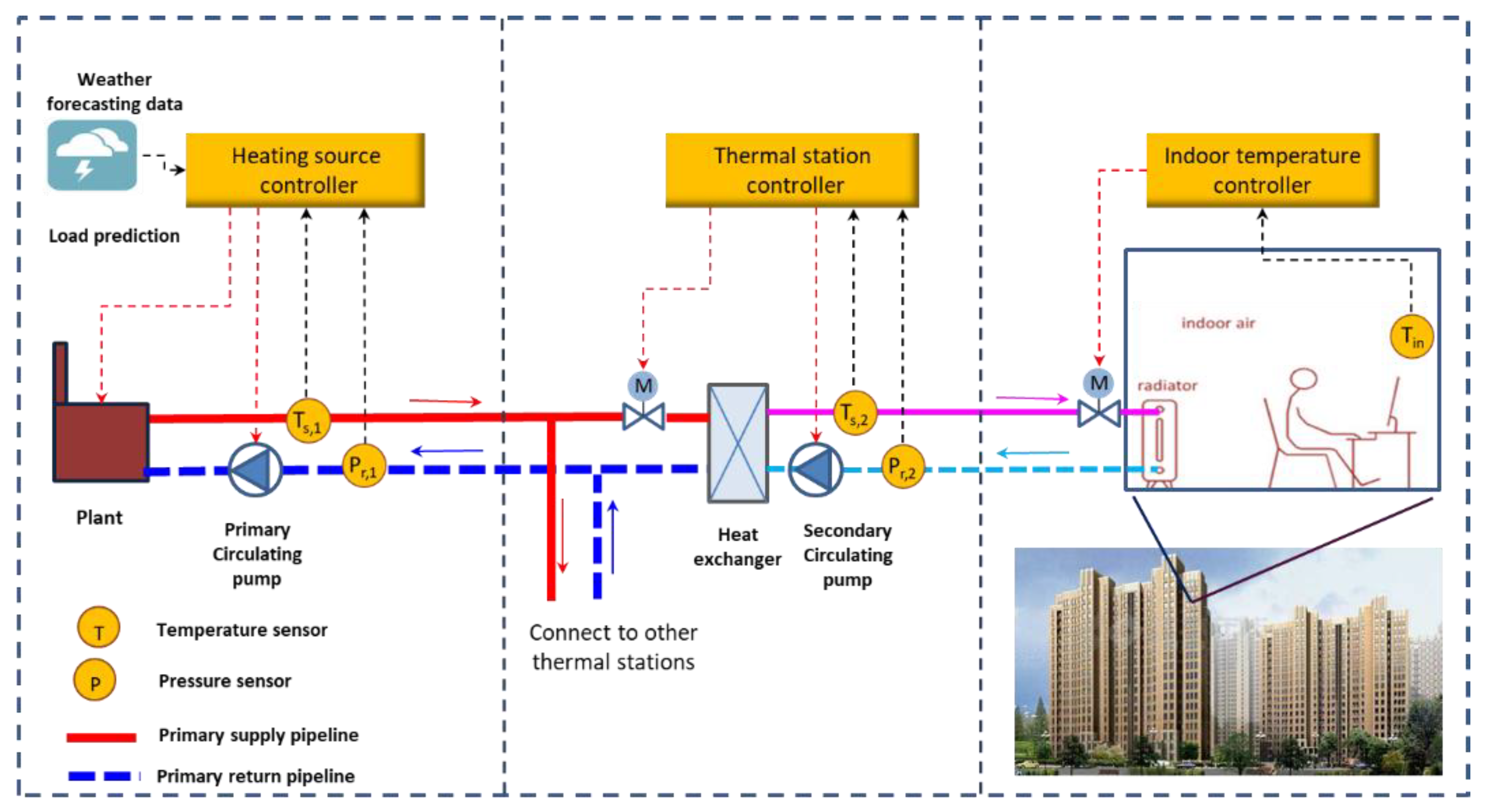
Figure 1 shows the schematic diagram of a typical indirectly connected DHS. In this heating system, the hot water in the primary network flows from the heat source to the heat exchangers of each heating station, then returns to the heat source after heating up the secondary water supply. In the secondary network, the outlet hot water from the heat exchangers is transported to the heating terminals of each building. The secondary-water-supply temperature is the most manipulated parameter used to tune the heat amount supplied to the buildings. The indoor temperature of the buildings represents the heating quality and can be used to adjust the set point of the secondary-supply temperature.

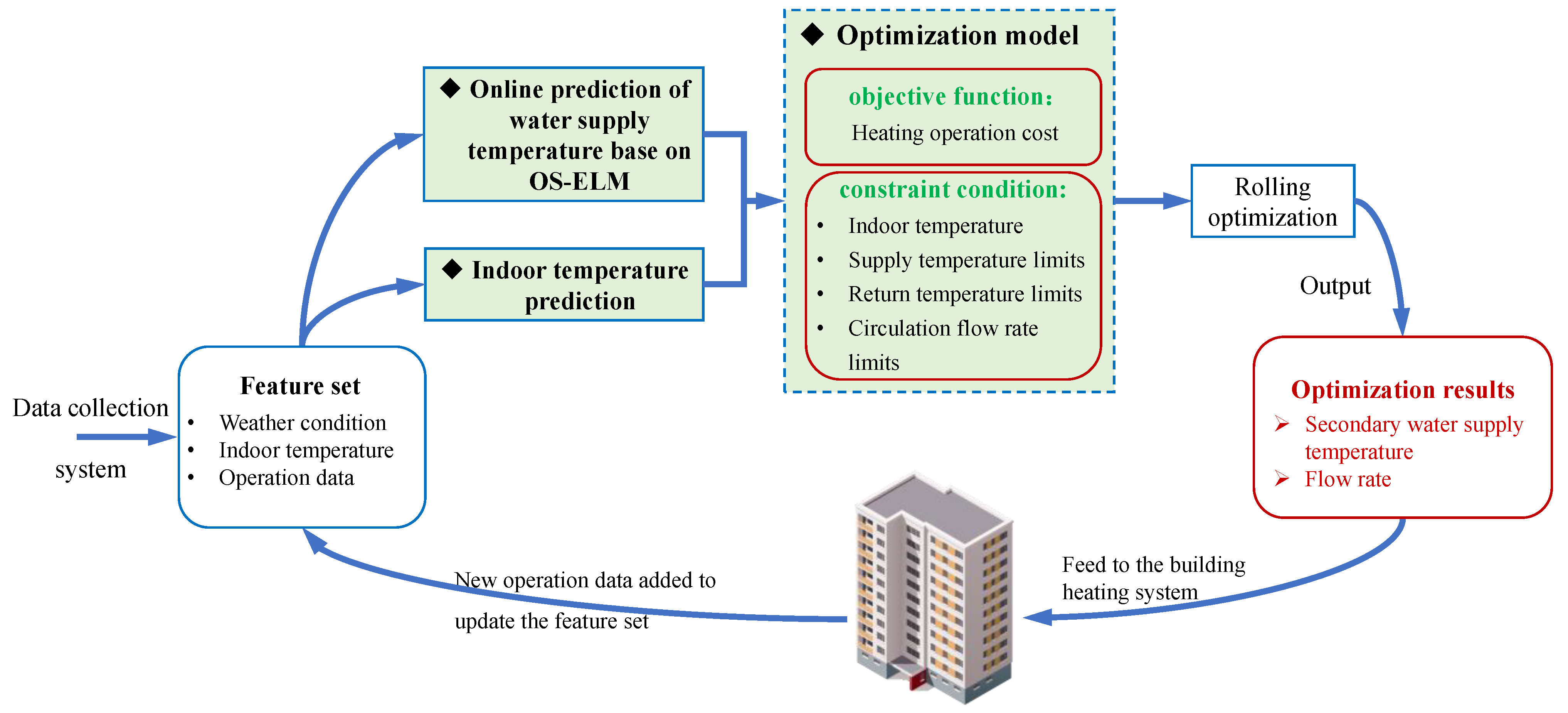
The overall operational optimization process framework of the system is shown in Figure 2. It mainly includes the four steps listed below.

(1) Parameters such as outdoor temperature, characteristic room temperature and secondary-network water-supply temperature are obtained from the heating monitoring platform, and the data are preprocessed.

(2) The temperature of the secondary water-supply network is dynamically predicted by online sequential extreme learning machine (OS-ELM). When the predicted secondary-network water-supply temperature is directly used as the set secondary-network water-supply temperature at the next time point, it conforms to the law of the secondary-network water-supply temperature of the thermal power station without optimal regulation, but it is impossible to judge whether the indoor temperature meets the needs of users under the set secondary-network water-supply temperature; that is, it is impossible to judge the rationality of setting the secondary-network water-supply temperature. Therefore, the indoor-temperature online prediction method is used to predict the characteristic indoor temperature to characterize the heating effect for a given water-supply temperature of the secondary network.

(3) Under the condition of meeting the thermal-comfort requirements of users, the operational energy-consumption cost of the heating system is minimized, and the water flow rate and supply temperature are adjusted accordingly. Then, the predicted secondary-network water-supply temperature and characteristic indoor-temperature parameters are substituted into the optimization control model for calculation, and the optimal secondary-network water-supply temperature and secondary-network flow parameters are obtained.

(4) The optimal secondary-network water-supply temperature and secondary-network flow parameters are used for the regulation of the thermal power station, and the feature set is updated through the feedback of the heated building. The time domain rolls forward as a whole. At the next sampling time point, new parameters are used to solve the optimization problem of updating the model; finally, the optimal compound regulation strategy for a certain period of time is obtained.

2.1. Water-Supply-Temperature Prediction Based on OS-ELM Method

Extreme learning machine (ELM) was developed from single-layer forward neural networks (SLFNs) as proposed by Huang et al. [21] in 2006. The purpose of this method is to minimize the training error value; the hidden layer does not need iteration, and the input weight and bias value can be selected at will. Research has shown that it has the ability to adapt to a large number of non-structural and imprecise laws that are characteristic of autonomous learning and optimal computing. For example, Sajjadi et al. [22] established nine short-term heat-load prediction models based on historical outdoor temperatures, historical heating load and historical primary-network return-water temperatures. The results showed that the prediction accuracy and generalization ability of limit learning machine (ELM) were better than BP neural networks and genetic algorithm optimization neural networks (GA-BPs). Guo et al. [23] used a correlation analysis and the lasso method to select 11 parameters, such as meteorological parameters, operating parameters, time and indoor temperatures. Based on the MLR, BP neural network, SVR and ELM methods, they predicted the heat load of a ground-source heat-pump system in the following 40 min. The results showed that the ELM model had the best prediction performance with a root mean square error of 3.824.

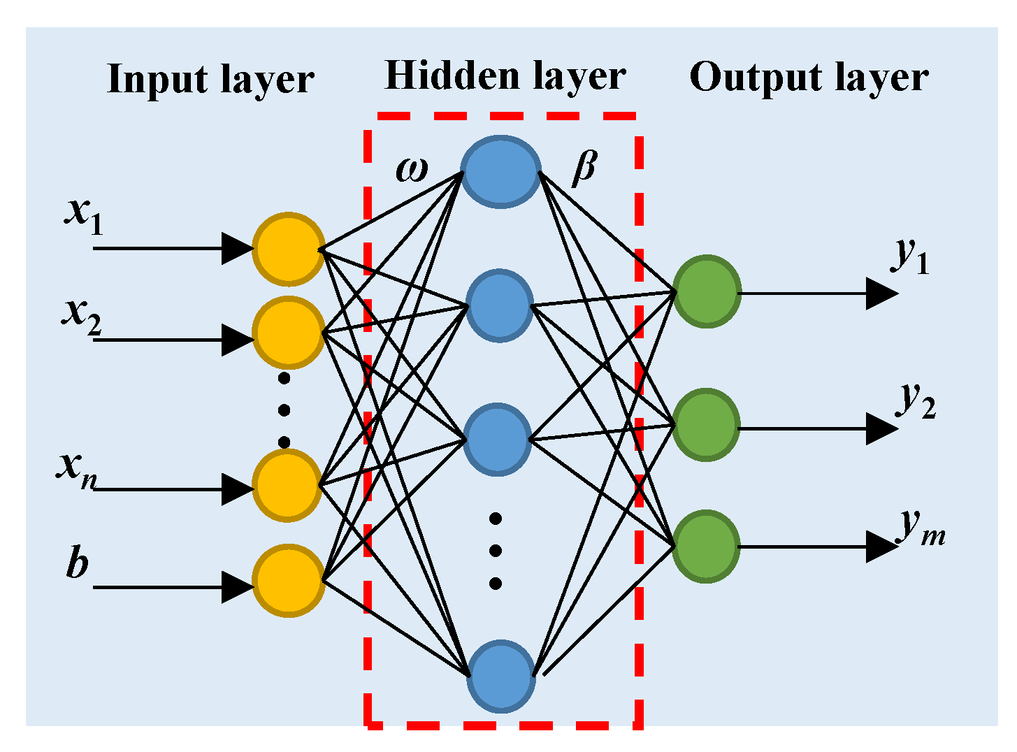
As shown in Figure 3, ELM generally comprises an input layer, a hidden layer and an output layer. Given n arbitrary groups of training samples (X_i, Y_i), where the input is X_i = [x₁, x₂, …, x_n]^T, and the output is Y_i = [y₁, y₂, …, y_m]^T, the output function of the hidden layer is Equation (1):

$$o_i={\displaystyle \sum _{i=1}^L{\beta }_{i}g({\omega }_i·x_j+b_i)},j=1,2,\cdots ,n$$

(1)

where β_i is the output weight; g(·) is the activation function; ω_i is the input weight; b_i is the bias of the i-th hidden layer; L is the number of hidden layers; and o_k is the i-th output.

The goal of the ELM algorithm is to minimize the difference between the output value of the model and the output value of the actual theory, as follows:

$${\displaystyle \sum _{i=1}^N\Vert o_i-y_i\Vert }=0$$

(2)

There exist β_i, ω_i and b_i satisfying Equation (3):

$${\displaystyle \sum _{i=1}^L{\beta }_{i}g({\omega }_i·x_j+b_i)}=y_j,j=1,2,\cdots ,n.$$

(3)

The matrix form of Equation (3) is as follows:

$$\mathit{\beta }\mathit{H}=\mathit{Y}$$

(4)

where H is the output matrix of the hidden layer; β is the output weight vector; and Y is the expected output vector.

The detailed description of Equation (4) is shown in Equations (5) and (6):

$$H({\omega }_1,\cdots ,{\omega }_L,b_1,\cdots ,b_L,X_1,\cdots ,X_n)={\left[\begin{array}{l}g({\omega }_1·X_1+b_1) \cdots g({\omega }_L·X_1+b_L)\\ ⋮ ⋮ \hspace{1em}\hspace{1em}\hspace{1em}\hspace{1em}\hspace{1em}\hspace{1em}⋮\\ g({\omega }_1·X_n+b_1) \cdots g({\omega }_L·X_n+b_L)\end{array}\right]}_{n\times L}$$

(5)

$$\mathit{\beta }={\left[\begin{array}{l}{\beta }_1^T\\ ⋮\\ {\beta }_L^T\end{array}\right]}_{L\times m},Y={\left[\begin{array}{l}{Y}_1^T\\ ⋮\\ Y_L^T\end{array}\right]}_{L\times m}$$

(6)

β can be obtained by solving Equation (7) using the least square method, as follows:

$$\Vert H\widehat{\beta }-Y\Vert =\Vert H{H}^{+}Y-Y\Vert =\underset{\beta }{\min }\Vert H\beta -Y\Vert$$

(7)

The least square solution is Equation (8):

$$\widehat{\beta }=H^{+}\mathit{Y}$$

(8)

where $\widehat{\beta }$ is the least square solution of the output weight vector and H⁺ is the Moore–Penrose generalized inverse of H.

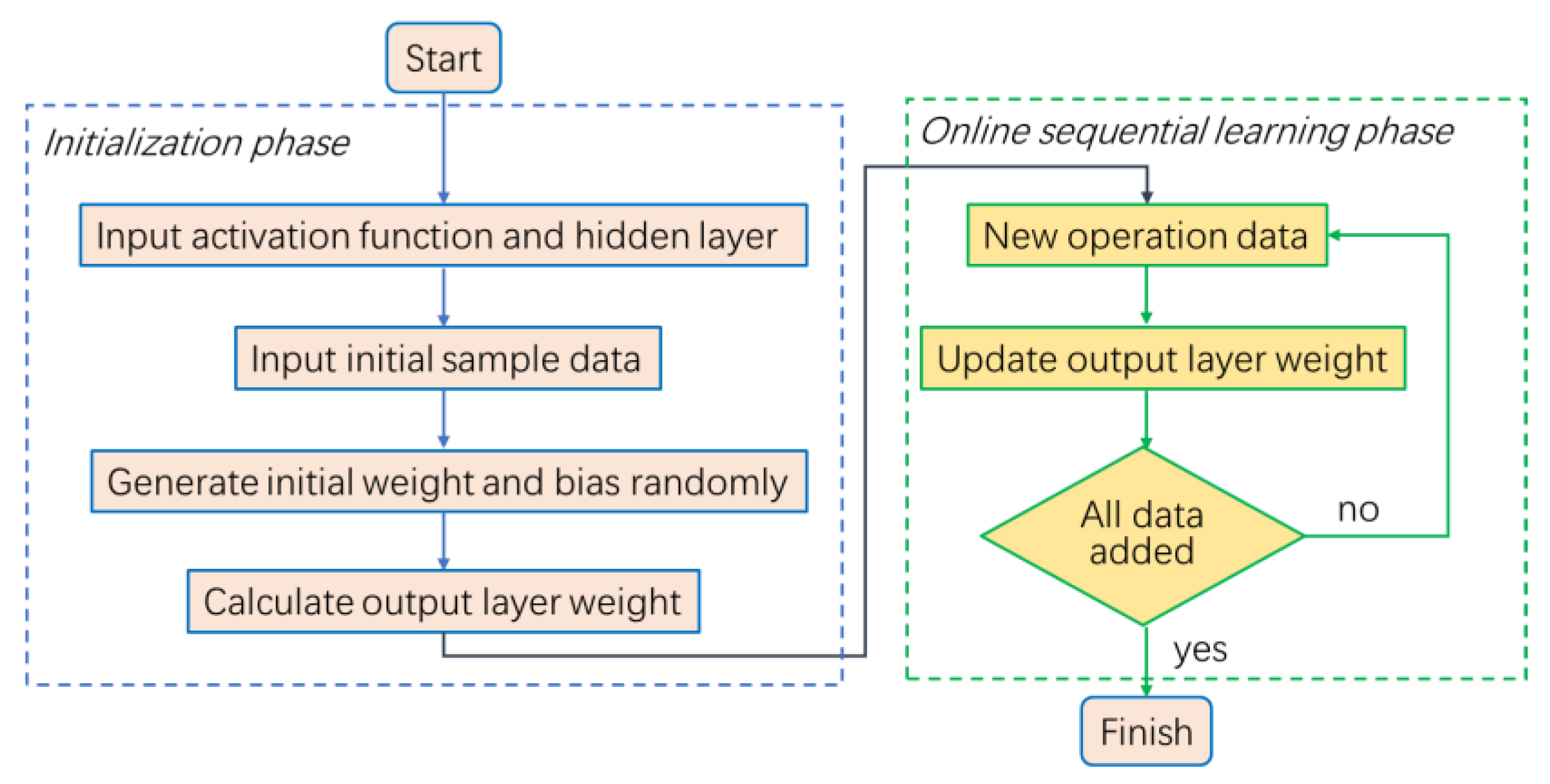
Online sequential extreme learning machine (OS-ELM) [24] is developed based on ELM combining an online learning mechanism. As the real operational condition of DHSs is dynamic, the performance of the original prediction model may decrease with time. Besides, in actual online prediction, the operational data are not able to be obtained to train the prediction model at once. When new data are added to the network, the ELM algorithm puts the new data and old data together to retrain the network; this takes a long time. Thus, we introduce a method which can add training data to the training model one by one or more and can lose the trained data to reduce space consumption. The specific implementation process of OS-ELM is mainly divided into two stages.

(1)

Initialization phase

The principle of the initialization stage is the same as that of the ELM algorithm. By giving the training samples, the number of neurons in the hidden layer, the excitation function, the input weight and the bias are randomly generated to determine the initial models, β₀ and H₀.

(2)

Online sequential learning phase

When a new batch of data is added to the model, the hidden layer output matrix and outp*ut weight vector can be updated according to Equation (9):

$$H_{t+1}={\left[\begin{array}{l}g({\omega }_1^T·X_1^{(t+1)}+b_1) \cdots g({\omega }_L^T·X_1^{(t+1)}+b_L)\\ \cdots \hspace{1em}\hspace{1em}\hspace{1em}\hspace{1em}\cdots \hspace{1em}\hspace{1em}\cdots \\ g({\omega }_1^T·X_{N_{t+1}}^{(t+1)}+b_1) \cdots g({\omega }_L^T·X_{N_{t+1}}^{(t+1)}+b_L)\end{array}\right]}_{n\times L}$$

(9)

$${\beta }_{t+1}={\beta }_t+K_{t+1}{H}_{t+1}(H_{t+1}^T-H_{t+1}^T{\beta }_t)$$

(10)

where the following definitions apply:

$$K_{t+1}=K_t-\frac{K_t{H}_{t+1}{H}_{t+1}^T{K}_t}{1+H_{t+1}^T{K}_t{H}_{t+1}}$$

(11)

$$K_0={(H_0^T{H}_0)}^{-1}$$

(12)

where N_t+1 represents the numbers of the t + 1-th sampling and $X_{N_{t+1}}^{(t+1)}=[x_1^{(t+1)},x_2^{(t+1)},\cdots ,x_{N_{t+1}}^{(t+1)}]$ is the input vector of the t + 1-th sampling.

Using the above equation and the newly added training data, H and β, all data are input; then, the training of the OS-ELM model is finally completed. The flowchart of OS-ELM is shown in Figure 4.

2.2. Prediction of Indoor Temperature

To predict the indoor temperature, we need to determine the functional relationship among outdoor temperature, historical indoor temperature, water-supply temperature, return-water temperature, flow rate and other parameters. It is necessary to establish a physical model to describe the thermal process of the building and use the model to obtain the functional relationship between other variables and the indoor temperature.

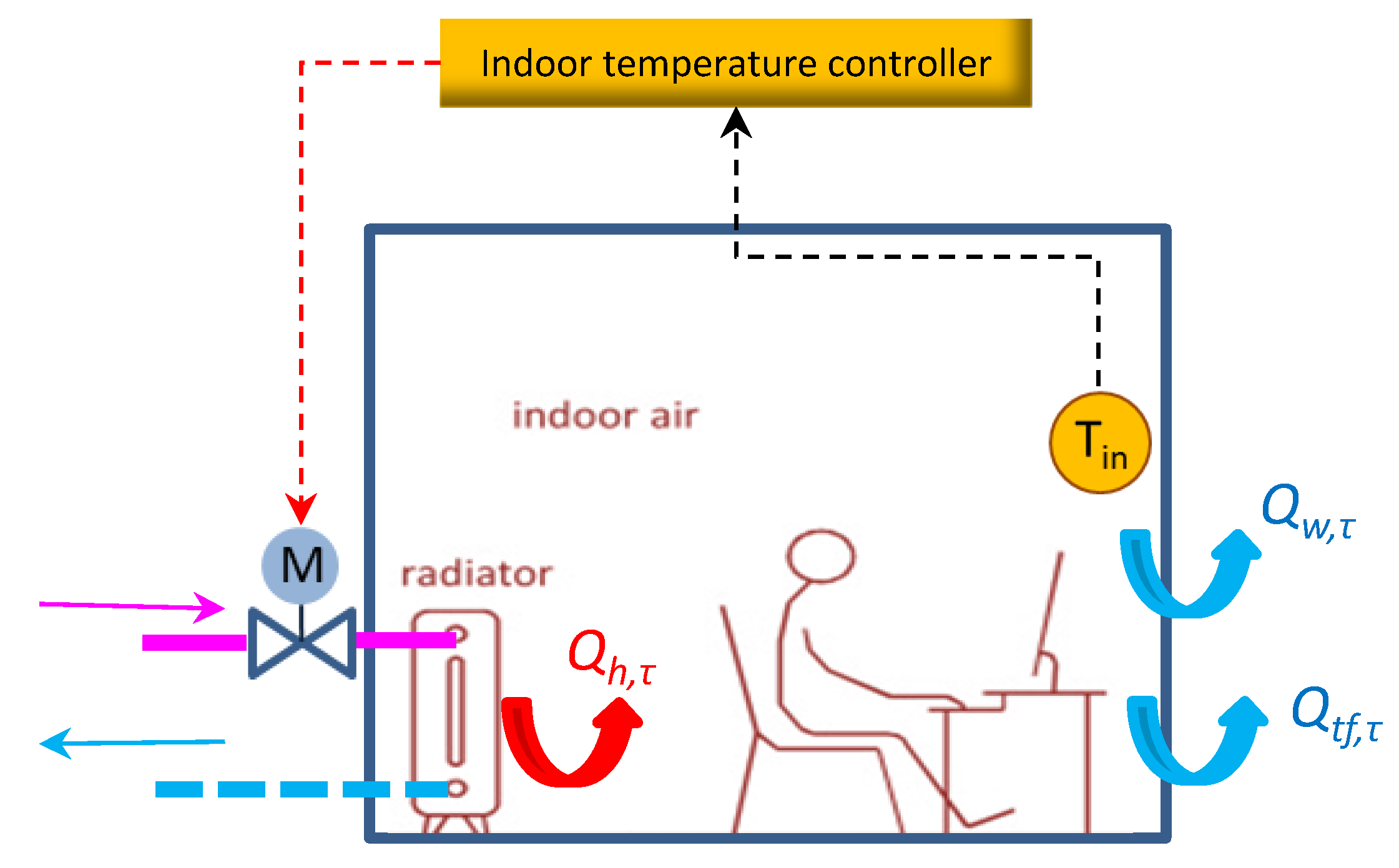
Figure 5 shows a simplified thermodynamic schematic of a heating room. According to the building heat-transfer theory, the heat gain of buildings at time τ is mainly the heat supply from the heating substation. The heat consumption at time τ is mainly composed of three parts, namely, heat loss across the building envelope, heating load caused by cold-air infiltration and cold-air intrusion. The building dynamic thermal process can be described by Equation (13):

$$\left({\rho }_{air}V{c}_{p,air}\right)\frac{d{T}_{in,\tau }}{d\tau }=Q_h{}_{,\tau }-Q_w{}_{,\tau }-Q_{tf,\tau }$$

(13)

where ρ_air is the indoor air density, kg/m³; V is the volume of the heating space, m³; c_p._air is the specific heat capacity of indoor air, J/(kg·K); T_in,τ is the indoor temperature at time τ, °C; Q_h,τ is the heat supplied by the network, W; Q_w,τ is the heating load across the building envelope, W; and Q_tf,τ is the heating load caused by cold-air infiltration and ventilation.

Equation (13) can be written as follows:

$$\left({\rho }_{air}V{c}_{p,air}\right)\frac{d{T}_{in,\tau }}{d\tau }=G_{\tau }{c}_{p,water}\left(T_{s,\tau }-T_{r,\tau }\right)-K_b{F}_b\left(T_{in,\tau }-T_{out,\tau }\right)$$

(14)

where G_τ is the secondary-water flow rate, kg/h; c_p,water is the specific heat capacity of hot water, c = 4187 J/(kg·°C); T_s,τ is the secondary-water-supply temperature, °C; T_r,τ is the secondary-return-water temperature, °C; K_b is the overall heat-transfer coefficient of the building envelope, W/(m²·°C); F_b is the overall heat-transfer area of the building envelope, m²; and T_out,τ is the outdoor temperature, °C.

Equation (14) can be simplified as follows:

$$\frac{d{T}_{in,\tau }}{d\tau }=a_1\left(T_{s,\tau }-T_{r,\tau }\right)-a_2\left(T_{in,\tau }-T_{out,\tau }\right)$$

(15)

where a₁ and a₂ are regression coefficients.

The differential expression of Equation (15) is:

$$\frac{T_{in}{}_{,\tau }-T_{in}{}_{,\tau -1}}{\Delta \tau }=a_1\left(T_s{}_{,\tau }-T_r{}_{,\tau }\right)-a_2\left(T_{in}{}_{,\tau }-T_{out}{}_{,\tau }\right)$$

(16)

where T_in,τ−1 is the indoor temperature at time τ − 1, °C.

Then, the indoor temperature at time τ can be calculated by Equation (17):

$$T_{in}{}_{,\tau }=c_1{T}_{in}{}_{,\tau -1}+c_2\left(T_s{}_{,\tau }-T_r{}_{,\tau }\right)+c_3{T}_{out}{}_{,\tau }$$

(17)

where c₁, c₂ and c₃ are coefficients that need solving.

There is an approximately linear function between the secondary-water-supply temperature and the return temperature, which can be written as Equation (18):

$$T_r=m_1·T_s$$

(18)

where m₁ is the fitting coefficient between the supply temperature and return temperature, which can be obtained by historical operational data.

Combining Equation (17) with Equation (18), the prediction expression of the indoor temperature of the heating station is:

$$T_{in}{}_{,\tau }=c_1{T}_{in}{}_{,\tau -1}+c_2(1-m_1)T_s{}_{,\tau }+c_3{T}_{out}{}_{,\tau }$$

(19)

c₁, c₂ and c₃ can be determined by the historical operational data of the heating station and the least square linear regression of multiple functions.

2.3. Optimization Model

The operational cost of heating systems mainly includes fuel cost, cost of electricity consumed by water pumps, water cost, labor cost, etc. As the cost of staff is relatively fixed, it can be used as a constant. The water-supply cost of the thermal power station is relatively small and can be ignored. From the perspective of the energy-saving benefits of heating, the operational cost of a heating system is mainly considered, including boiler fuel cost and cost of electricity consumed by the circulating pump. For the heating system using a gas-fired boiler, the objective functions of the system-operation energy-consumption equation are represented by Equations (20)–(22):

$$C_{total}=c_{gas}{E}_{gas}+c_{power}{E}_{power}$$

(20)

$$E_{gas}=\frac{3600Q}{{\eta }_{gas}(1-{\eta }_1)(1-{\eta }_2)q_{d,gas}}$$

(21)

$$E_{power}=\frac{s}{3.6\times {10}^6\times {\eta }_{pump}}{\left(\frac{G}{\rho }\right)}^3$$

(22)

where C_total is the total operational cost, yr; c_gas is the unit price of natural gas, yr/m³; E_gas is the consumption of natural gas, m³; c_power is the unit price of electricity, yr/kWh; E_power is the power consumption of the circulation pumps, kWh; Q is the consumer heat load, kW; q_d,gas is the low calorific value of natural gas, kJ/m³; η_g is the efficiency of the gas-fired boiler; η₁ is the heat-loss ratio of the primary network; η₂ is the heat-loss ratio of the secondary network; s is the resistance characteristic coefficient of the secondary network, Pa/(m³/h)²; G is the mass flow rate of secondary circulation water, kg/h; ρ is the water density, kg/m³; and η_pump is the pump efficiency.

Constraint Condition

In the actual operation of a central heating system, the parameters of supply- and return-water temperatures and water-supply flow of the secondary network are not infinite but within a certain reasonable value range. The setting of these parameters should not only meet the heating needs of users but also take into account the economy of the heating pipe network. It is this range limit that constitutes the constraint condition of the system-operation energy-consumption equation. The constraints of this subject mainly include the aspects listed below.

(1)

Water-supply temperature of secondary network

$$T_{s,\min }\le T_s\le T_{s,\max }$$

(23)

where T_s,min is the lower-limit value of the secondary-supply temperature, °C; and T_s,max is the upper-limit value of the secondary-supply temperature, °C.

(2)

Flow rate of secondary network

$$G_{\min }\le G\le G_{\max }$$

(24)

where G_min is the lower-limit value of the secondary flow rate, kg/h; and G_max is the upper-limit value of the secondary flow rate, kg/h.

(3)

Return temperature

$$T_{r,\min }\le T_r\le T_{r,\max }$$

(25)

where T_r,min is the lower-limit value of the secondary-return temperature, °C; and T_r,max is the upper-limit value of the secondary-return temperature, °C.

(4)

Indoor temperature

In order to improve the thermal comfort of users, it is considered that the indoor temperature can meet the thermal needs of users within the set indoor temperature ±0.5 °C; the indoor-temperature constraints are as follows:

$$\left|T_{in}-T_{in,}{}_{set}\right|\le 0.5$$

(26)

where T_in,set is the set point of the indoor temperature, °C.

(5)

Heat-balance equation

When the operation of the heating pipe network is stable, if the heat loss along the heating pipe network is ignored, the heat load required by the user and the heating capacity of the heating station are equal. It can be approximately considered that there is the following heat balance in a heating cycle:

$$Q=1.163G\left(T_s-T_r\right)=K_b{F}_b\left(T_{in}-T_{out}\right)$$

(27)

where K_b is the overall heat-transfer coefficient of the building envelope, W/(m²∙°C); and F_b is the envelope area, m².

To sum up, the objective function and constraints of the system-operation energy consumption are:

$$\begin{array}{l}\min C_{total}=c_{gas}\times \frac{3600\times 1.163G(T_s-T_r)}{{\eta }_{gas}(1-{\eta }_1)(1-{\eta }_2)q_{d,gas}}+c_{power}\times \frac{s}{3.6\times {10}^6\times {\eta }_{pump}}{\left(\frac{G}{\rho }\right)}^3\\ s.t. \{\begin{array}{l}{T}_{s,\min }\le T_s\le T_{s,\max }\\ T_{r,\min }\le T_r\le T_{r,\max }\\ G_{\min }\le G\le G_{\max }\\ \left|T_{in}-T_{in,}{}_{set}\right|\le 0.5\\ 1.163G\left(T_s-T_r\right)-K_b{F}_b\left(T_{in}-T_{out}\right)=0\end{array}\end{array}$$

(28)

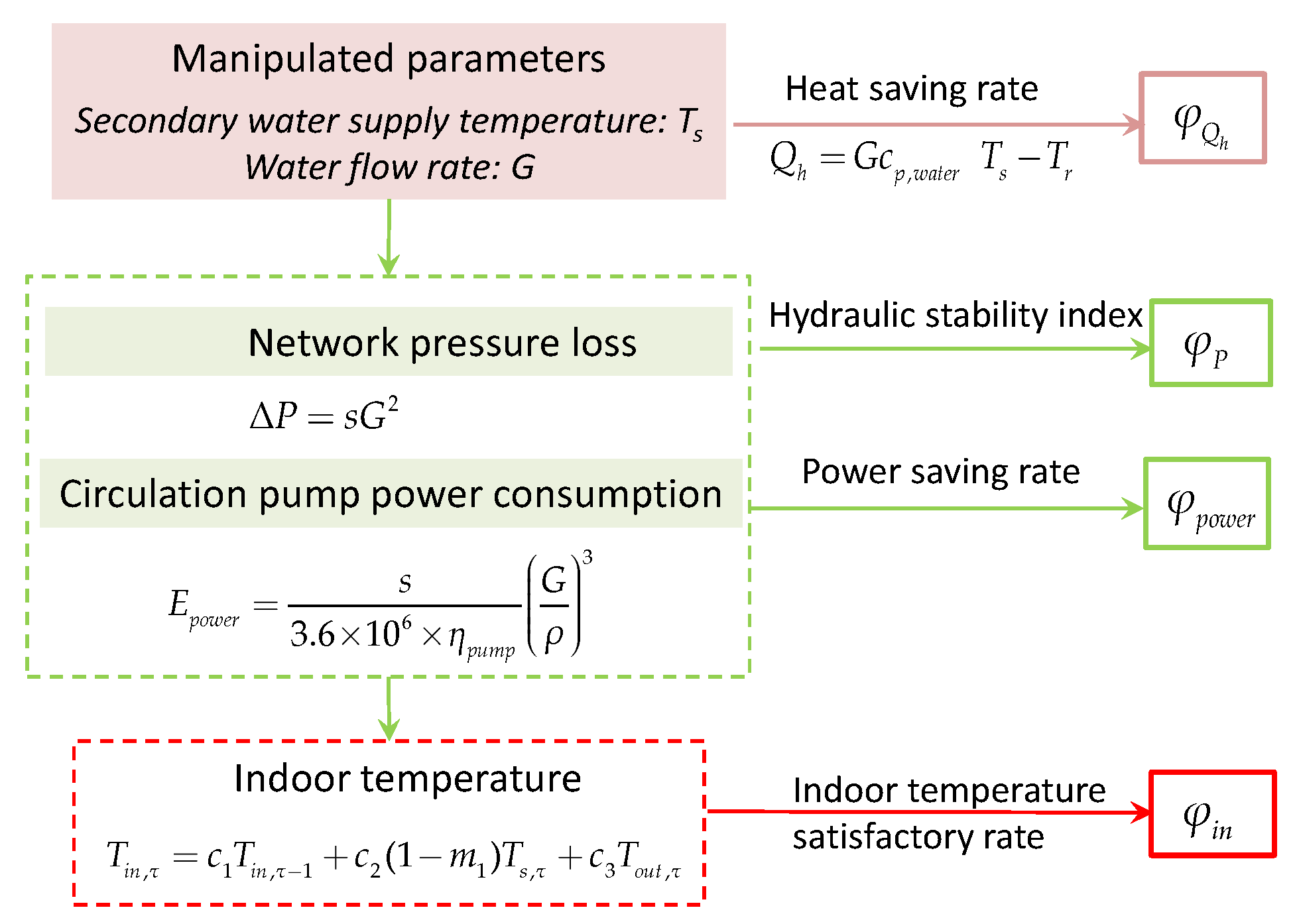
2.4. Evaluation Indices

The regulation method proposed in this paper manipulates the secondary-water-supply temperature and water flow rate to reduce energy consumption. In order to evaluate its performance, this paper proposes 4 indices from the perspectives of heating-saving rate, indoor-temperature satisfactory rate, power-saving rate and hydraulic stability. The relationships between these indices and the operational parameters are as shown in Figure 6.

2.4.1. Heat-Saving Rate

The heat-saving rate (${\phi }_{Q_h}$) is the deviation percentage between the hourly or daily corrected heat consumption before the regulation of the heating system and the hourly or daily corrected heat consumption after the regulation of the heating system. The higher the ${\phi }_{Q_h}$ value is, the more energy is saved. The calculation method is as follows:

$${\phi }_{Q_h}=\frac{Q_{h,norm}^b-Q_{h,norm}^a}{Q_{h,norm}^b}\times 100\%$$

(29)

where $Q_{h,norm}^a$ is the normalized heat consumption after regulation, GJ; and $Q_{h,norm}^b$ is the normalized heat consumption after regulation of the heating system, GJ.

Equation (30) is used to calculate the corrected heat consumption:

$$Q_{h,norm}=Q_{meter}\frac{20-T_{out,des}}{T_{in,ave}-T_{out}}$$

(30)

where Q_meter is the actual heat consumption recorded by the heat meter, GJ; Q_h,norm is the normalized heat consumption, GJ; T_in,ave is the cumulative average characteristic indoor temperature, °C; T_out represents the average outdoor temperature in different heating periods, °C; and T_out,des is the designed outdoor average temperature, °C.

2.4.2. Indoor-Temperature Satisfactory Rate

This is the standard rate of the imported indoor temperature and is denoted by φ_in. The higher the indoor-temperature compliance rate, the higher the heating quality of the thermal power station. The calculation method is shown in Equation (31):

$$\begin{array}{l}{U}_i=\{\begin{array}{l}1 \left|T_{in}-T_{in,set}\right|\le 1\\ 0 \left|T_{in}-T_{in,set}\right|>1\end{array}\\ {\phi }_{in}=\frac{{\displaystyle \sum U_i}}{n}\times 100\%\end{array}$$

(31)

where φ_in represents the indoor-temperature satisfactory rate, %; U_i is the number of users whose indoor temperature meets the standard; and n is the number of normal-heating users.

2.4.3. Power-Saving Rate

The power-saving rate (φ_power) is the deviation percentage between the hourly or daily corrected power consumption before the regulation of the heating system and the hourly or daily corrected power consumption after the regulation of the heating system. The calculation method is as follows:

$${\phi }_{power}=\frac{E_{power,norm}^a-E_{power,norm}^b}{E_{power,norm}^a}\times 100\%$$

(32)

where $E_{power,norm}^a$ is the hourly or daily corrected power consumption of the circulating water pump in the secondary network before regulation, kWh; and $E_{power,norm}^b$ is the hourly or daily corrected power consumption of the circulating water pump in the secondary network after regulation, kWh.

The corrected power consumption is calculated using Equation (33):

$$E_{power,norm}=E_{power,meter}\frac{20-T_{out,des}}{T_{in,ave}-T_{out}}$$

(33)

where E_power,meter is the actual power consumption of the circulating water pump of the secondary network in different heating periods recorded by metering, kWh; and E_power,norm is the corrected heat consumption of the circulating water pump of the secondary network in different heating periods, kWh.

2.4.4. Hydraulic-Stability Index

Standard deviation is usually used to reflect the dispersion degree of a data set. Therefore, in this paper, a standard deviation value is used as index φ_P to measure the hydraulic stability of the pipe network. The calculation method is as follows:

$$P_{ave}=\frac{{\displaystyle \sum _{i=1}^n{P}_i}}{n}$$

(34)

$${\phi }_P=\sqrt{\frac{1}{n}{\displaystyle \sum _{i=1}^n{(P_i-P_{ave})}^2}}$$

(35)

where n is the number of times required to collect the water-supply pressure (differential pressure between supply and return water) of the pipe network; P_i is the water-supply pressure at time i (differential pressure between supply and return water), bar; and P_ave is the average value of the water-supply pressure (differential pressure between supply and return water) over n times, bar.

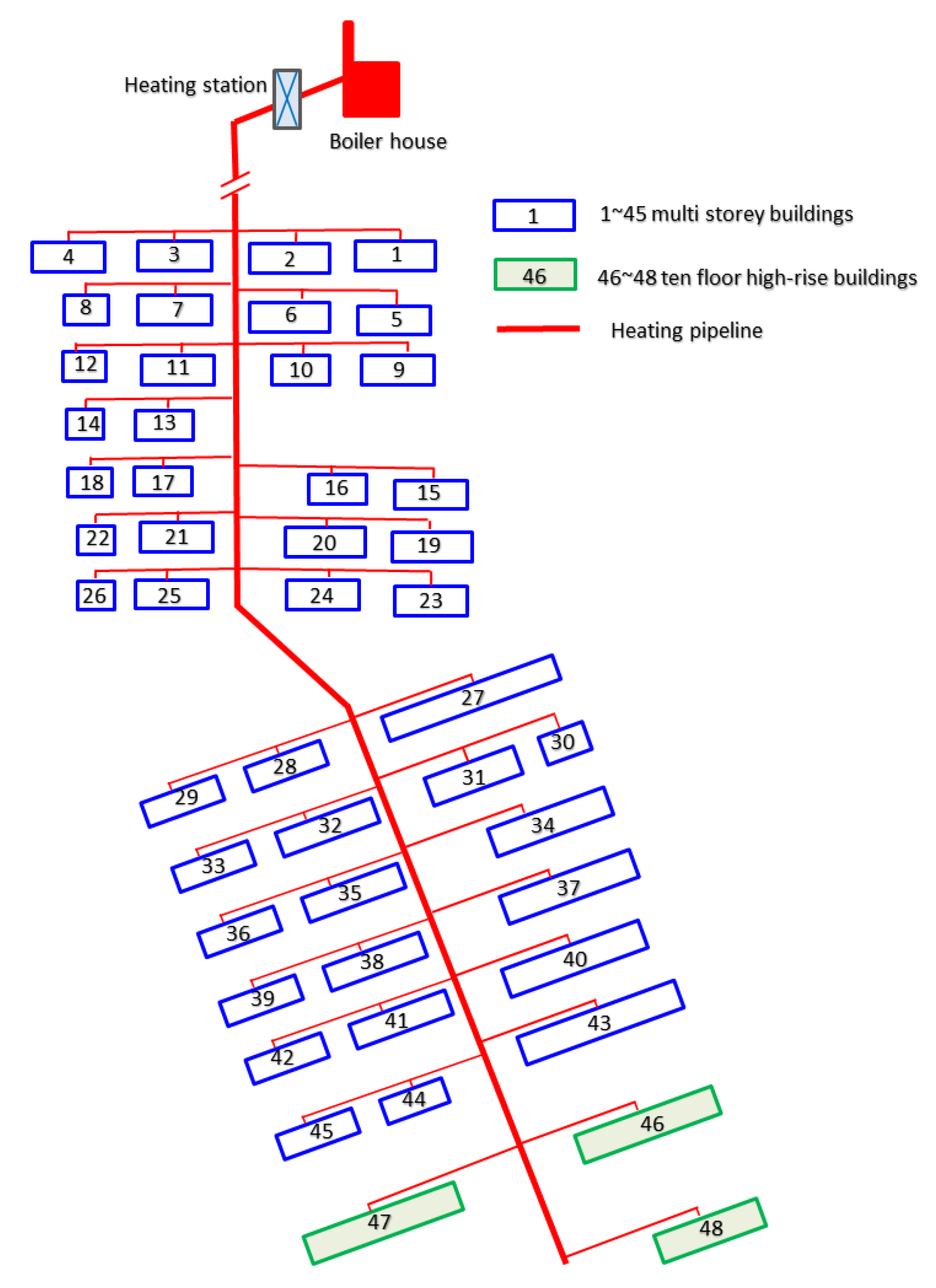
3. Case Study

The heating system of a teacher’s apartment in North China was selected as the research object. The layout of the studied system is shown in Figure 7. The total construction area where the teacher’s apartment is located is 190,000 m², with 48 buildings in total, of which buildings 46#–48# are 3 high-rise buildings (10 floors) with a floor height of 2.8 m, and the remaining 45 buildings are villas and multi-story buildings. The heating terminals are radiators, and the designed pressure bearing capacity is 0.4 MPa.

The configuration of the heating system is as follows: a horizontal condensing gas-fired hot-water boiler with a heat source of 14 MW. The heat source and the secondary network are indirectly connected by plate heat exchangers. The basic information related to the system are listed in

Table 1. Parameters of the studied heating system.

No.	Parameter	Value	Unit
1	designed water-supply temperature of boiler	105	°C
2	designed return-water temperature of boiler	75	°C
3	rated flow rate of boiler	300	m3/h
4	designed secondary-water-supply temperature	75	°C
5	designed secondary-return-water temperature	50	°C
6	rated flow of secondary-network circulating pump	506	m3/h
7	rated power of secondary-network circulating pump	90	kW
8	rated efficiency of secondary-network circulating pump	75	%
9	unit price of gas *	2.4	yr/m3
10	electricity price *	0.74	yr/kWh
11	boiler efficiency	90	%
12	low calorific value of gas	35,982.4	kJ/m3
13	heat-loss rate of the primary network **	0	%
14	heat-loss rate of the secondary network	10	%
15	resistance coefficient of pipe network	0.177	m3/s
16	water density	983.2	kg/m3

* The local gas price in the 2018–2019 heating season. ** As the primary network of the heating system is set inside the boiler house, the heat loss of the primary network can be ignored.

.

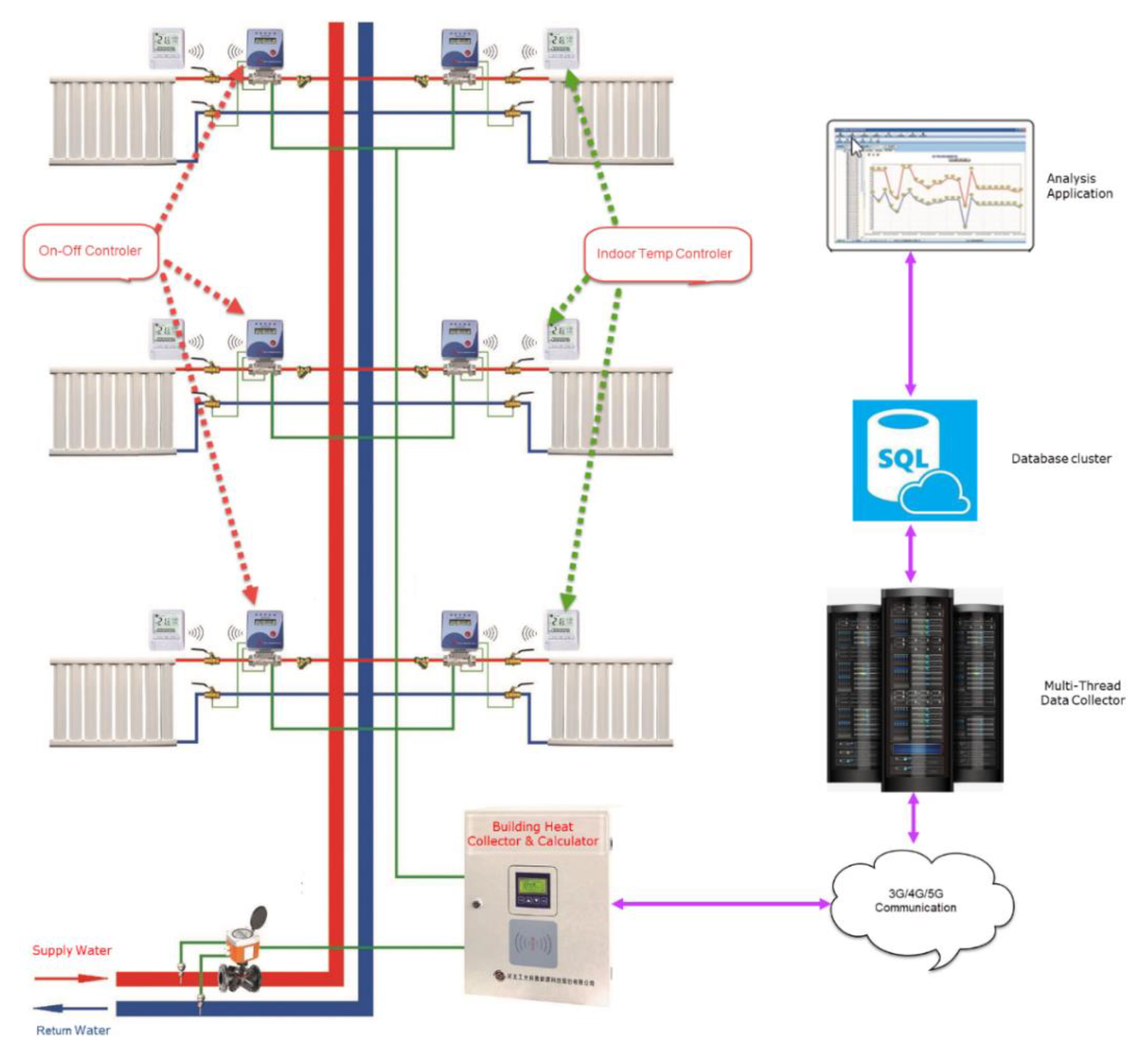
The heating system studied in this paper is equipped with an integrated intelligent system of heat metering and temperature control, as shown in Figure 8. The system equipment includes a household heat meter, an intelligent on–off temperature control valve, an indoor-temperature controller and a data collector. An ultrasonic heat meter is installed at the thermal inlet of the user to calculate the heat consumption of the user. The intelligent control valve and wireless indoor-temperature controller are installed in the user’s living room. After the user sets the indoor temperature through the indoor-temperature controller, the intelligent control valve controls the opening and closing of the valve by comparing the set value of the indoor temperature with the actual value, so as to provide users with heating on demand. The data acquisition concentrator can collect the accumulated flow of the user’s heat meter, the supply- and return-water temperatures, the instantaneous flow, the indoor temperature, the user-set temperature, the opening and closing statuses of the intelligent on–off valve and the opening and closing time of the temperature control valve. It adopts GPRS (general packet radio service) remote data transmission and has the function of local storage of historical data. Finally, all the collected heating data are transmitted to the intelligent heating-network energy-saving monitoring platform through the network to guide the operational regulation of the heating station.

The collected data mainly include outdoor temperatures, indoor temperatures, secondary-network water-supply temperatures, secondary-return-water temperatures, instantaneous flow and supply–return pressure difference. The user indoor-temperature acquisition frequency is 2 h, and the acquisition frequency of the other heating parameters is 10 min. In order to unify the sampling period, the outdoor temperature, the secondary-network water-supply temperature, the flow and the supply and return pressure difference are treated as average values of the 2 h period. The heating data of the heating station in the community from 16 November 2018 to 15 March 2019 and from 15 November 2019 to 21 November 2020 were selected as samples, with a total of 1524 groups of data.

3.1. Water-Supply-Temperature Prediction Results

In this paper, the factors affecting the water-supply temperature of the secondary network include outdoor temperature T_out, indoor temperature T_in, instantaneous flow G, supply and return pressure difference ΔP and historical secondary-network water-supply temperature T_s,τ-n. Pearson correlation coefficient r and PACF [25] are used to select the input variable of the prediction model. The results are the outdoor temperatures and the historical secondary-network water-supply temperatures 28 h before the prediction time.

The collected operational data are divided into training set and test set. The data from 16 November 2018 to 25 February 2019 (1224 groups data; 93.6% of the total data) are the training set. The data from 26 February 2019 to 4 March are the test set (84 groups data; 6.4% of the total data).

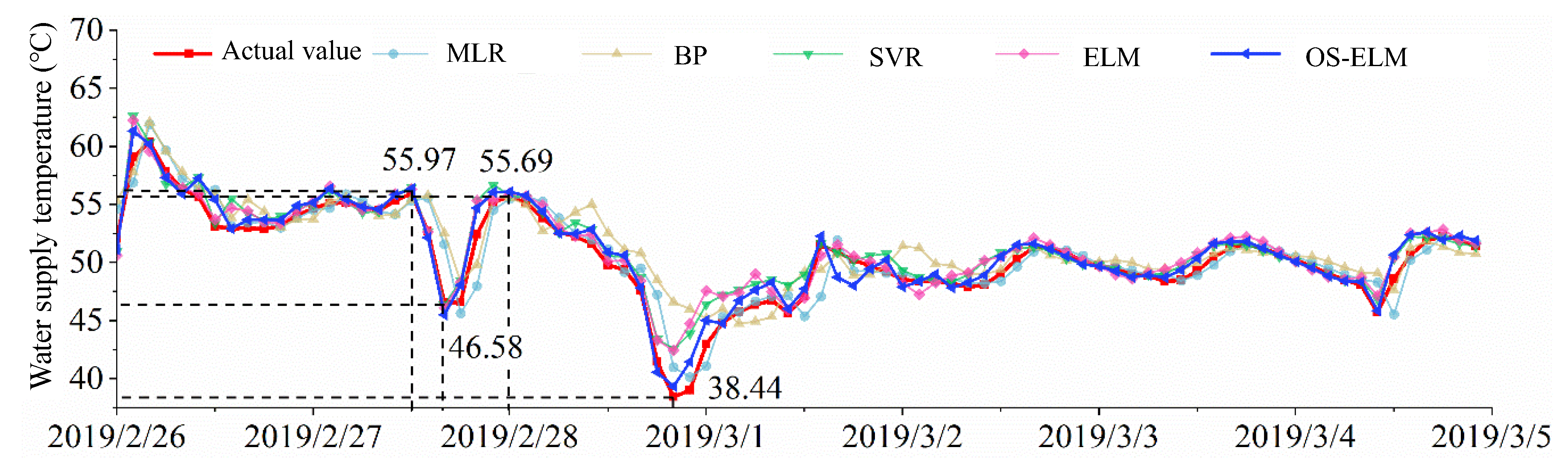
The comparison between the predicted curve and the actual curve of the secondary-network water-supply temperatures is shown in Figure 9. For 26 February and 1–4 March, the fluctuation range of the water-supply temperatures of the secondary network is small, and the prediction curves of the five models are close to the actual curves. The water-supply temperature of the secondary network fluctuates greatly from 27 to 28 February. The maximum water-supply temperature values of the secondary network on 27 and 28 February are 55.97 °C and 55.69 °C, respectively, and the minimum water-supply temperature values are 46.58 °C and 38.44 °C, with fluctuation ranges of 9.39 °C and 17.25 °C. For 27 February, the water-supply temperature curve of the secondary network predicted by the ELM, SVR and OS-ELM models is close to the actual curve, while the effects of BP and MLR are poor. The prediction curve of OS-ELM is the closest one to the actual curve for 28 April.

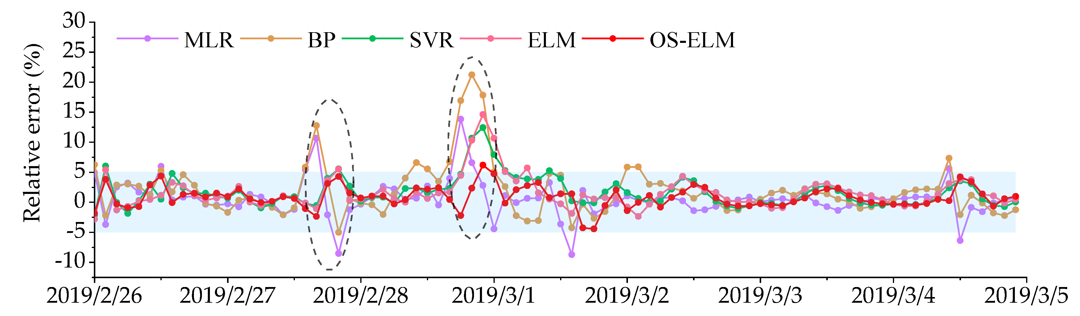
The comparison of the relative errors of the five prediction models is shown in Figure 10. It can be seen from Figure 10 that, for 26 February and 1–4 March, the prediction relative errors of the five models remain within ± 5%, meeting the error requirements. For 27 February, the absolute maximum relative errors of the MLR, BP neural network, SVR and ELM models are 10.69%, 12.26%, 5.58% and 5.52%, respectively, while the relative errors of the OS-ELM model remain within ± 5%. For 28 February, the predicted values of MLR, BP neural network, SVR and ELM fluctuate greatly compared with the actual values, and the maximum relative errors are 13.86%, 21.23%, 12.46% and 14.63%, respectively, while the maximum relative error of the OS-ELM model is 6.20%. When the water-supply temperatures of the secondary network fluctuate greatly, the prediction accuracy of the OS-ELM model is higher than that of the other four models.

3.2. Indoor-Temperature Prediction Results

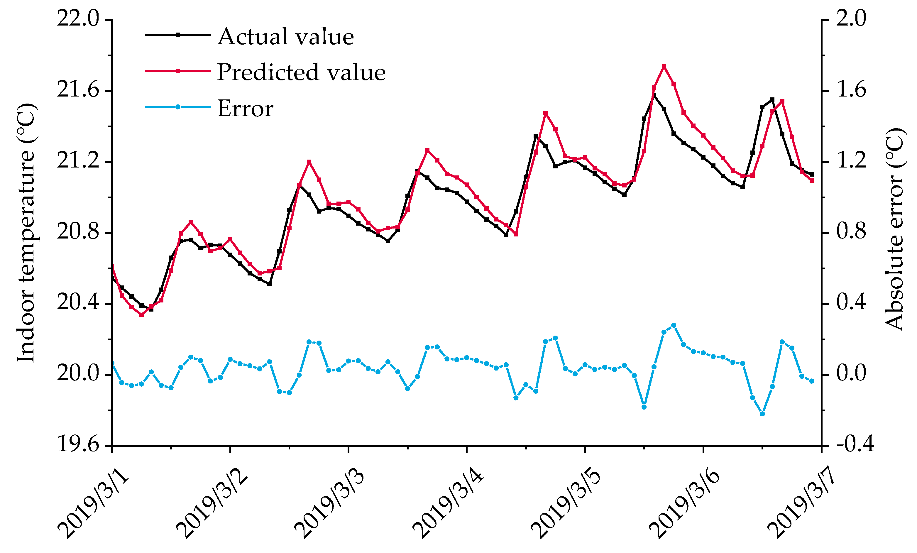
Through the least square regression of the coefficient in Equation (19), the equation of the indoor-temperature prediction model of the thermal power station is finally obtained as follows:

$$T_{in}{}_{,\tau }=0.978T_{in}{}_{,\tau -1}+0.008T_s{}_{,\tau }+0.012T_{out}{}_{,\tau }$$

(36)

The prediction results of Equation (36) are compared with the actual indoor temperatures in Figure 11. It can be seen that the predicted values are in good agreement with the measured values. The minimum absolute error and maximum absolute error are −0.22 °C and 0.21 °C. It can be considered that the prediction accuracy is acceptable to predict the indoor temperature.

3.3. Results of Optimization Model of Heating System

The efficiency of the circulating water pump is affected by the operating flow of the pipe network. The relationship between the efficiency and flow of the secondary-network water pump of the thermal power station can be obtained by using the regression analysis method:

$${\eta }_{pump}=-3.78\times {10}^{-6}{G}^2+3.81\times {10}^{-3}G-0.22$$

(37)

Combined with the heating parameters of the heating system, the objective function of the system-operation energy-consumption equation is:

$$C_{total}=2.4\times \frac{4186.8G(T_s-T_r)}{2.915\times {10}^7}+0.74\times \frac{0.177}{-13.608G^2+13716G-7.92\times {10}^5}{\left(\frac{G}{983.2}\right)}^3$$

(38)

For the actual situation of the studied pipe network, the step-change limit of the secondary-water-supply temperature of ±5 °C, i.e., the constraint on the secondary-supply temperature, is:

$$\left|T_{s,\tau +1}-T_{s,\tau }\right|\le 5$$

(39)

where T_s,τ+1 is the predicted secondary-water-supply temperature at the next time point, °C.

To ensure the safe and stable operation of the heating network, the actual water flow rate of the secondary network is 80–120% of the rated flow:

$$0.8G_r\le G\le 1.2G_r$$

(40)

where G_r is the rated flow of the secondary-network circulating pump, kg/h.

Considering the characteristics of the heat exchangers in the heating station and the economy of the whole project, combined with the operational experience relative to other heat networks, the upper and lower limits of the return-water temperature are determined as 30 °C and 55 °C:

$$30\le T_r\le 55$$

(41)

The user indoor-temperature setting law at a different time can be obtained, that is, the user-set indoor temperature at each time has a certain limit. Combined with the indoor-temperature prediction model, it is considered that the indoor temperature varies within the set points ±0.5 °C. The indoor-temperature limit is written as follows:

$$\left|0.978T_{in}{}_{,\tau -1}+0.008T_s{}_{,\tau }+0.012T_{out}{}_{,\tau }-T_{in}{}_{,set}\right|\le 0.5$$

(42)

To sum up, the operational energy-consumption equation of a heating system under actual working conditions is shown in Equation (43):

$$\begin{array}{l}\min C_{total}=2.4\times \frac{4186.8G(T_s-T_r)}{2.915\times {10}^7}+0.74\times \frac{0.177}{-13.608G^2+13716G-7.92\times {10}^5}{\left(\frac{G}{983.2}\right)}^3\\ s.t.\{\begin{array}{l}\left|T_{s,\tau +1}-T_{s,\tau }\right|\le 5\\ 30\le T_r\le 55\\ 404800\le G\le 607200\\ \left|0.978T_{in}{}_{,\tau -1}+0.008T_s{}_{,\tau }+0.012T_{out}{}_{,\tau }-T_{in}{}_{,set}\right|\le 0.5\\ 1.163G\left(T_s-T_r\right)-K_b{F}_b\left(T_{in}-T_{out}\right)=0\end{array}\end{array}$$

(43)

4. Results and Discussion

To analyze the control effect of the proposed method, two consecutive days, 4 March 2018 and 5 March 2018, were selected for an experimental comparative analysis. The former day, operated without the new method, is marked as before regulation, while the latter, to which the proposed integrated control method is applied, is recorded as after regulation.

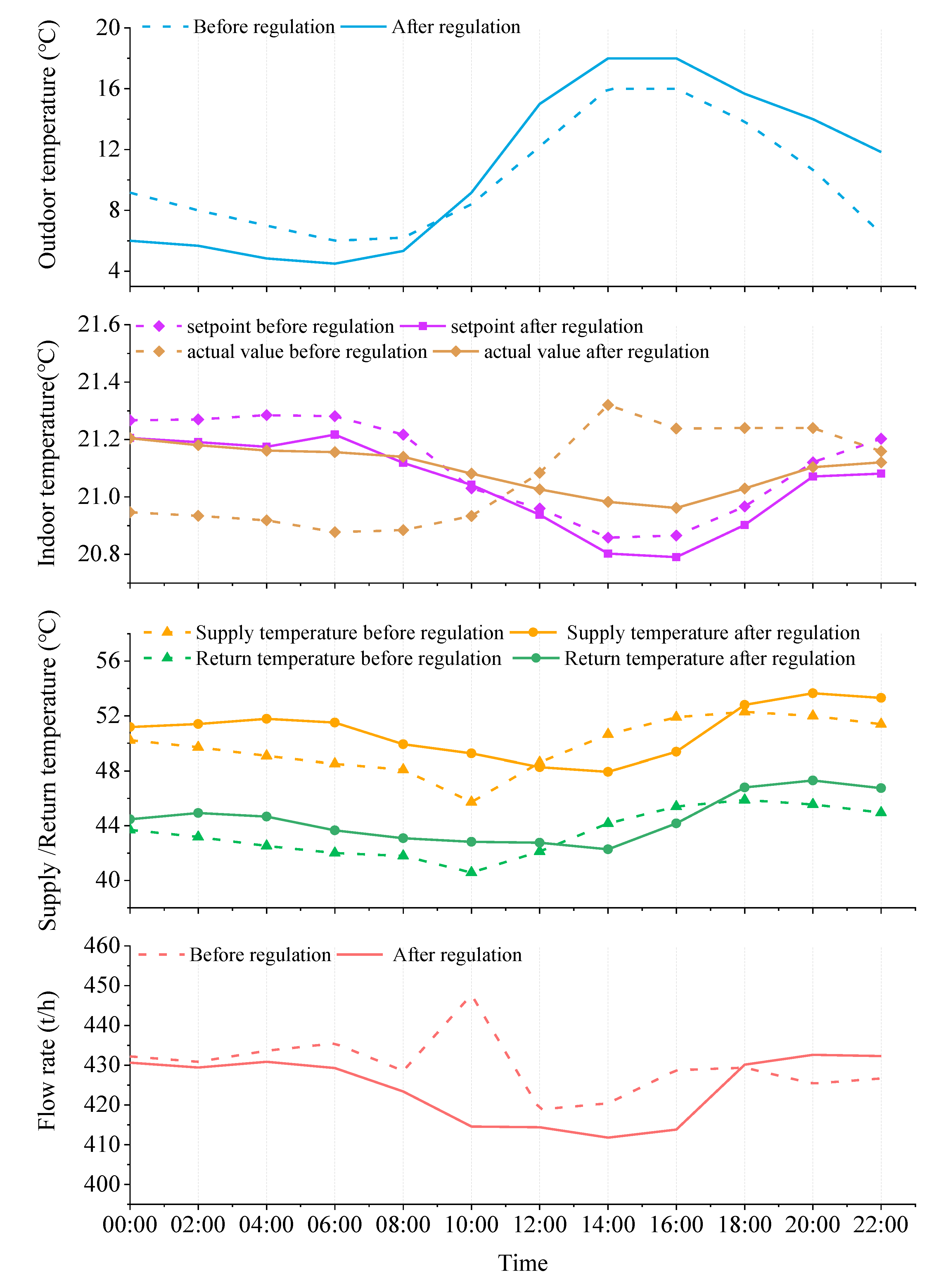
4.1. Comparison of Operational Parameters

Figure 12 shows the changes in the main operating parameters of the heating system when two operational strategies are adopted. Before regulation, the water-supply temperature of the secondary network changes between 45.7 and 52.3 °C. The flow-variation range of the circulating pump in the secondary network is 418.8 to 447.7 t/h, and the average flow rate is 429.8 t/h. The average user-set indoor temperature remains almost unchanged from 0:00 to 6:00, decreases from 8:00 to 14:00 and gradually increases after 16:00. The actual user indoor temperature is quite different from the set point. There is insufficient heating from 0:00 to 10:00, when the outdoor temperature is low, and excessive heating after 12:00. This means that the water-supply temperature of the secondary network is not regulated according to the requirements of the user-set indoor temperature, indicating that the operation before regulation does not provide the required on-demand heating.

After regulation, the secondary-water-supply temperature changes in an approximately opposite way with respect to that of the outdoor temperature, which is consistent with the change law of the indoor-temperature set point, and the change range is 47.9 to 53.7 °C. The flow-rate variation is 411.8 to 432.6 t/h, and the average flow is 424.4 t/h. In addition, the user-set indoor-temperature rule after regulation is similar to that before regulation, and users have a certain energy-saving behavior. The variation law of the actual user indoor temperature after regulation is close to the set point, and the deviation is small, in the range −0.1 to 0.2 °C, which proves that the proposed regulation strategy can better meet user demand for heating on demand.

4.2. Indoor-Temperature Comparison

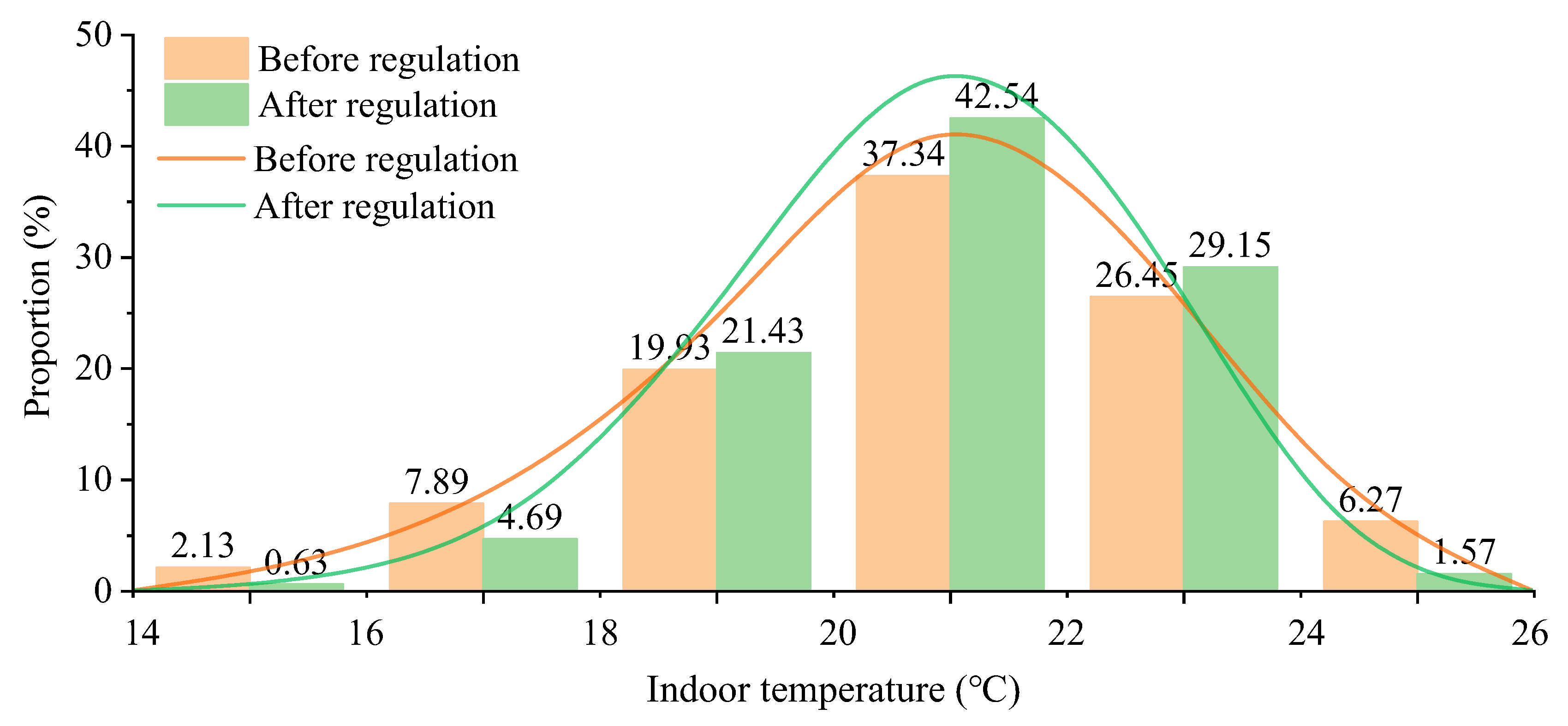
The distribution of user indoor temperatures before and after regulation are here statistically analyzed, as shown in Figure 13. The user indoor temperatures approximately present a normal distribution. Before regulation, 37.34% are in the range 20 to 22 °C; 9.32% are lower than 18 °C; 6.27% are higher, in the range 24 to 26 °C. After regulation, 42.54% are distributed in the range 20 to 22 °C, which is 5.2% higher than the temperature range before regulation. Meanwhile, both lower-indoor-temperature users (lower than 18 °C) and overheated users (higher than 24 °C) decrease. Lower-indoor-temperature users decrease from 9.32% to 5.32%, while overheated users decrease from 6.27% to 1.57%. The calculated indoor-temperature satisfactory rates are 72.86% after regulation, with 20.87% being higher than that before regulation. This shows that, after regulation, thermal comfort is improved, and the occurrence of overheating or supercooling decreases.

4.3. Energy-Saving Effect

The heat- and power-consumption performances before and after regulation are analyzed and compared in this section.

Figure 14 shows the heat consumption every 2 h under the two operational strategies. After the normalization of heat consumption, the heat consumption before regulation fluctuates in the range 31.06 to 84.23 GJ, while it fluctuates in the range 29.63 to 71.28 GJ every 2 h after regulation. The heat consumption of the integrated regulation strategy proposed in this paper is significantly lower than that before regulation. After regulation, the heat-saving rate varies in the range 3.29 to 16.24%. From 12:00 to 16:00, when the outdoor temperature is high, the heat-saving rate exceeds 10%. After regulation, the energy-saving effect is obvious. The equivalent daily heat consumption before regulation is 545.81 GJ, while it is 495.01 GJ after regulation. The equivalent daily heat consumption after regulation is 50.80 GJ lower than before regulation, and the heat-saving rate is 16.33.

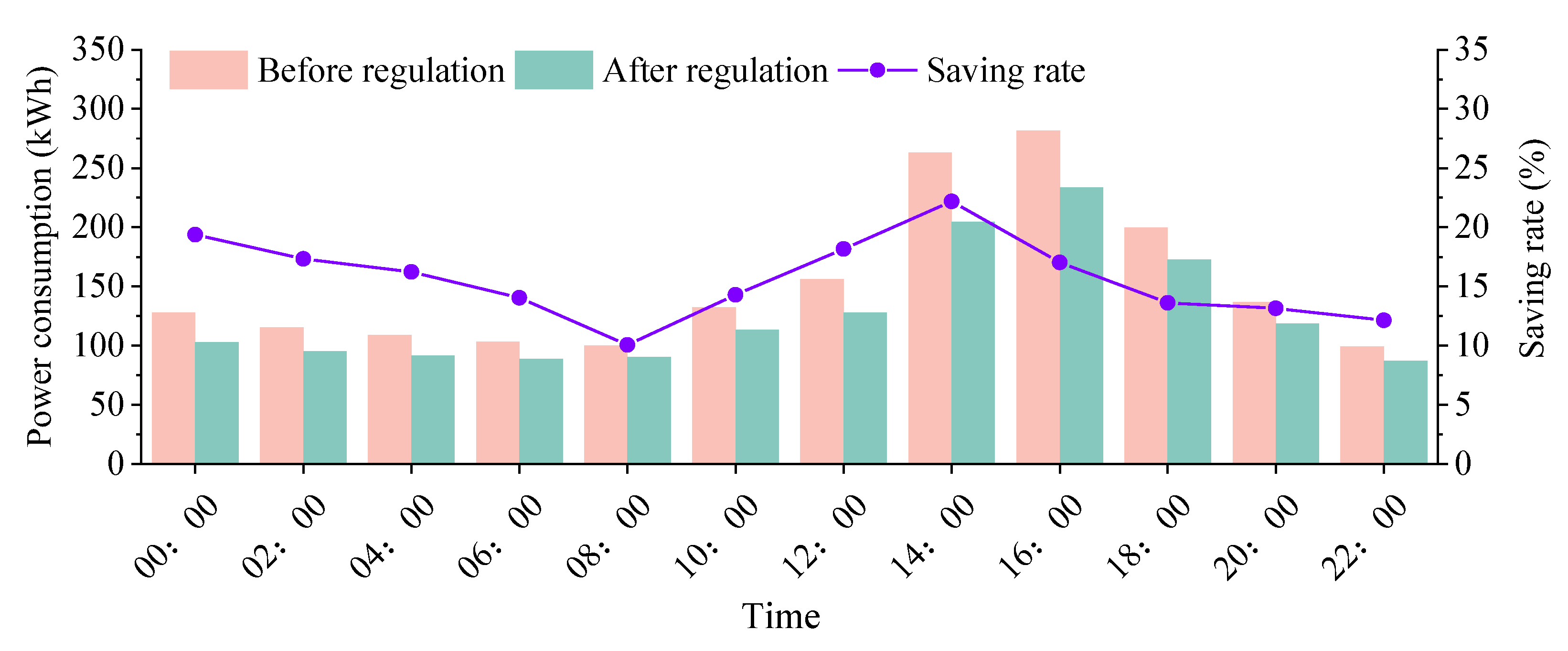
Figure 15 shows the power consumption of the secondary circulating water pump every 2 h under the two operational strategies. After the conversion of the power consumption values to the same level, the power consumption before regulation fluctuates in the range 99.33 to 281.60 kWh, and the power consumption every 2 h after regulation fluctuates in the range 87.28 to 233.62 kWh. The power consumption after regulation is significantly lower than that before regulation. After regulation, the power-saving rate varies in the range 10.06 to 22.18%. The equivalent daily power consumption before regulation is 1825.32 kWh, and that after regulation is 1527.32 kWh. The equivalent daily power consumption after regulation is 279.99 kWh lower than that before regulation, and the power-saving rate is 16.33%.

4.4. Network Hydraulic-Stability Analysis

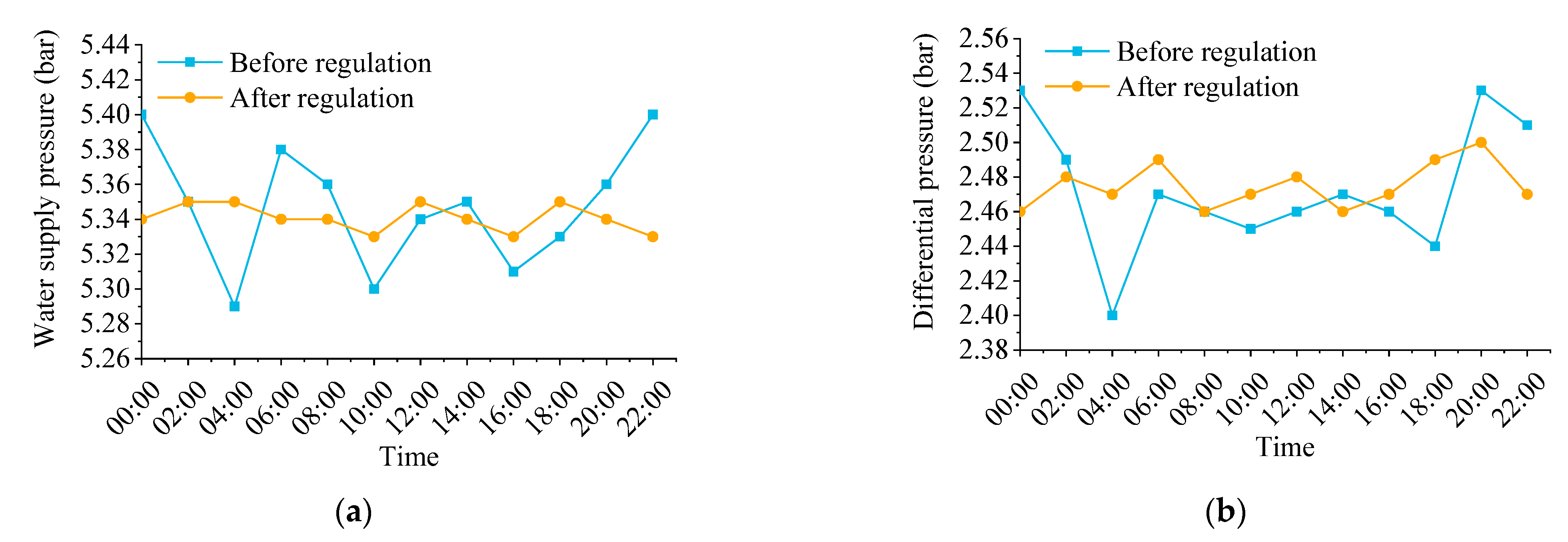
As shown in Figure 16, the water-supply pressure of the secondary network before regulation is in the range 5.35 ± 0.05 bar, while it is in a narrower range, 5.34 ± 0.01 bar, after regulation. The change in the differential pressure between supply and return water is similar; it fluctuates in the range 2.46 ± 0.07 bar before regulation and in the range 2.48 ± 0.02 bar after regulation. In addition, according to Equation (35), the SD values of supply pressure and differential pressure before regulation are 0.034 and 0.036, while they are 0.008 and 0.013, respectively, after regulation. The results show that the fluctuations in the water-supply pressure and differential pressure of the secondary network are significantly reduced after adopting the regulation strategy proposed in this paper.

5. Conclusions

Firstly, combining secondary-side water-supply-temperature prediction and the indoor-temperature prediction model of the thermal power station, this paper studies the compound regulation strategy of the heating system. Combined with the actual heating system, the operational energy-consumption-cost equation of the heating system is established on the premise that ensuring heating quality and meeting the conditions of the actual supply- and return-water temperatures and the flow range of the heating pipe network are fundamental. Aiming at minimizing the operational cost of the heating system, the heating operational parameters are optimized, and a refined on-line regulation strategy is formulated.

The regulation strategy is applied to a typical heating system for verification. The operational effect of the thermal power station is evaluated in terms of heat-saving rate, indoor-temperature compliance rate, power-saving rate and hydraulic-stability index, respectively. The results show that the operational regulation strategy can give reasonable heating parameters according to the heat demand of users, with obvious energy-saving effects and good practical application.

The field study results show that the operation executed with the regulation strategy proposed in this paper obtains 9.31% heat saving rate, 16.33% power saving rate and indoor-temperature satisfactory rate increasing by 20.87% than that without an energy-saving regulation strategy. The fluctuations in the water-supply pressure and differential pressure of the secondary network are significantly reduced, and the energy-saving effect is obvious.