
Thermo-Energy Performance of Lightweight Steel Framed Constructions: A Case Study


Abstract
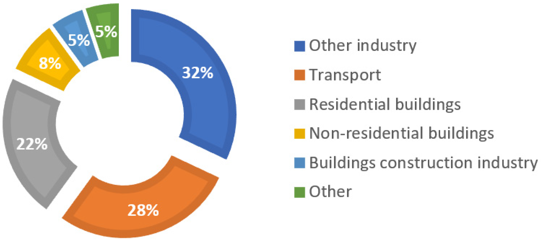
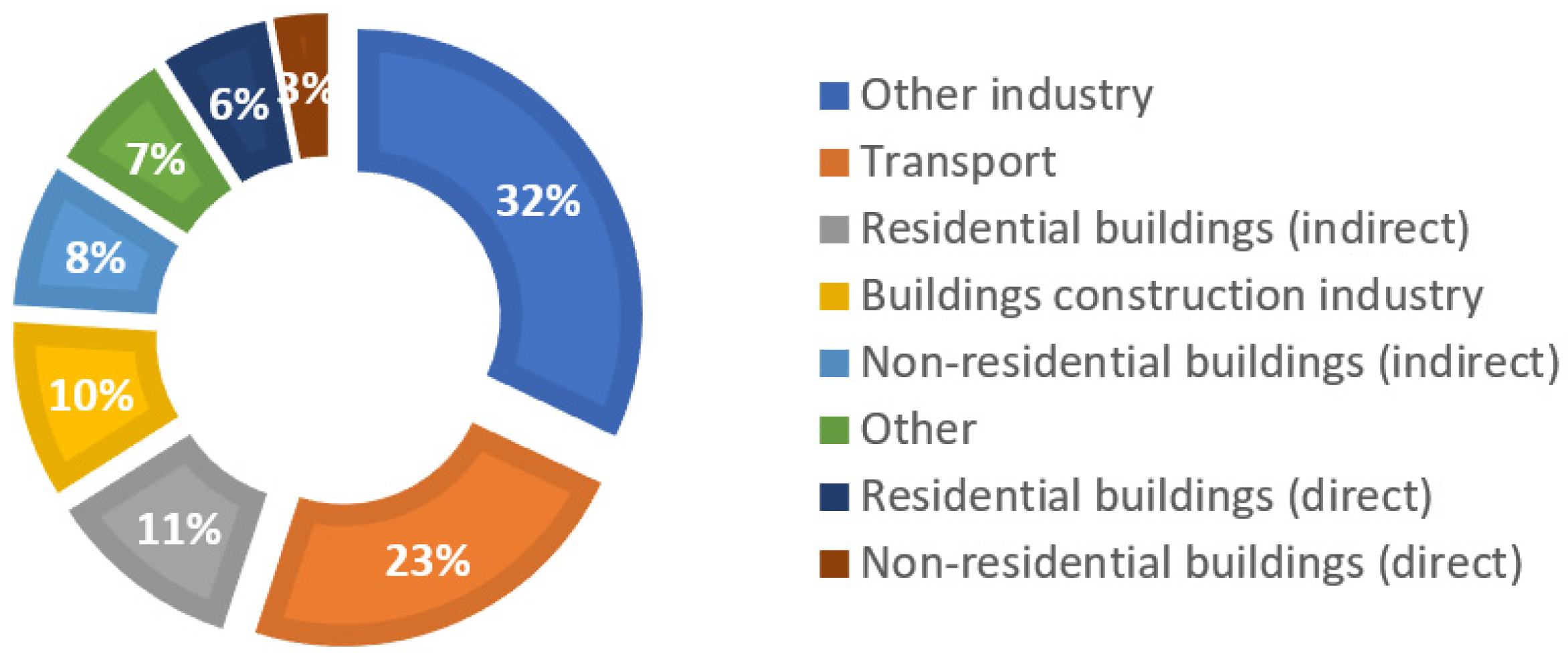
:1. Introduction
2. The Case Study
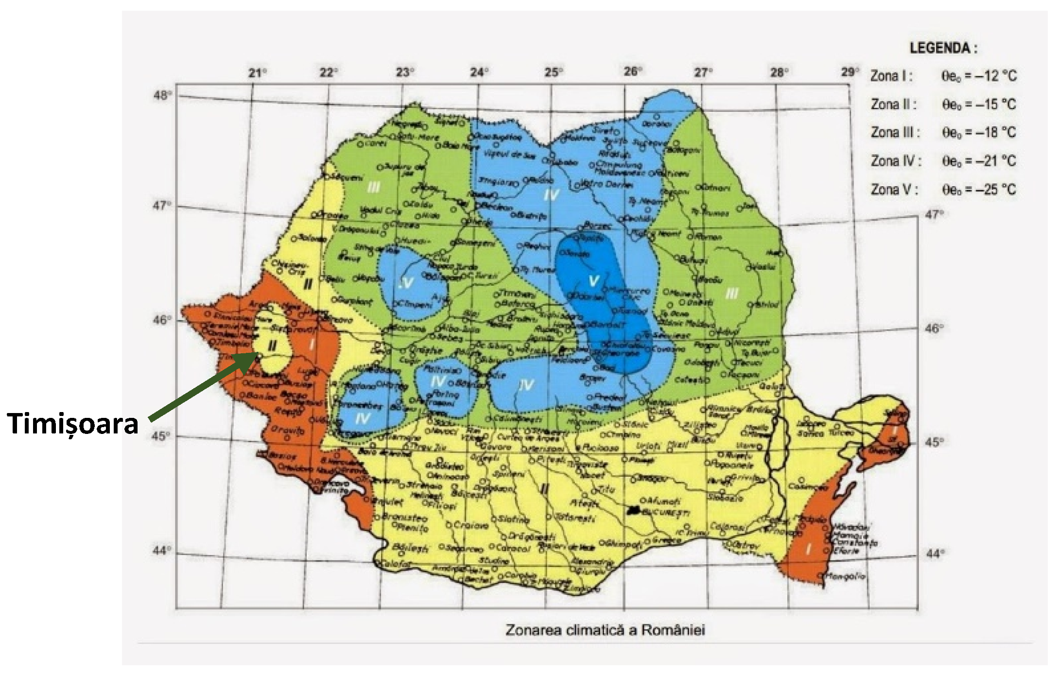
2.1. Site and Climate
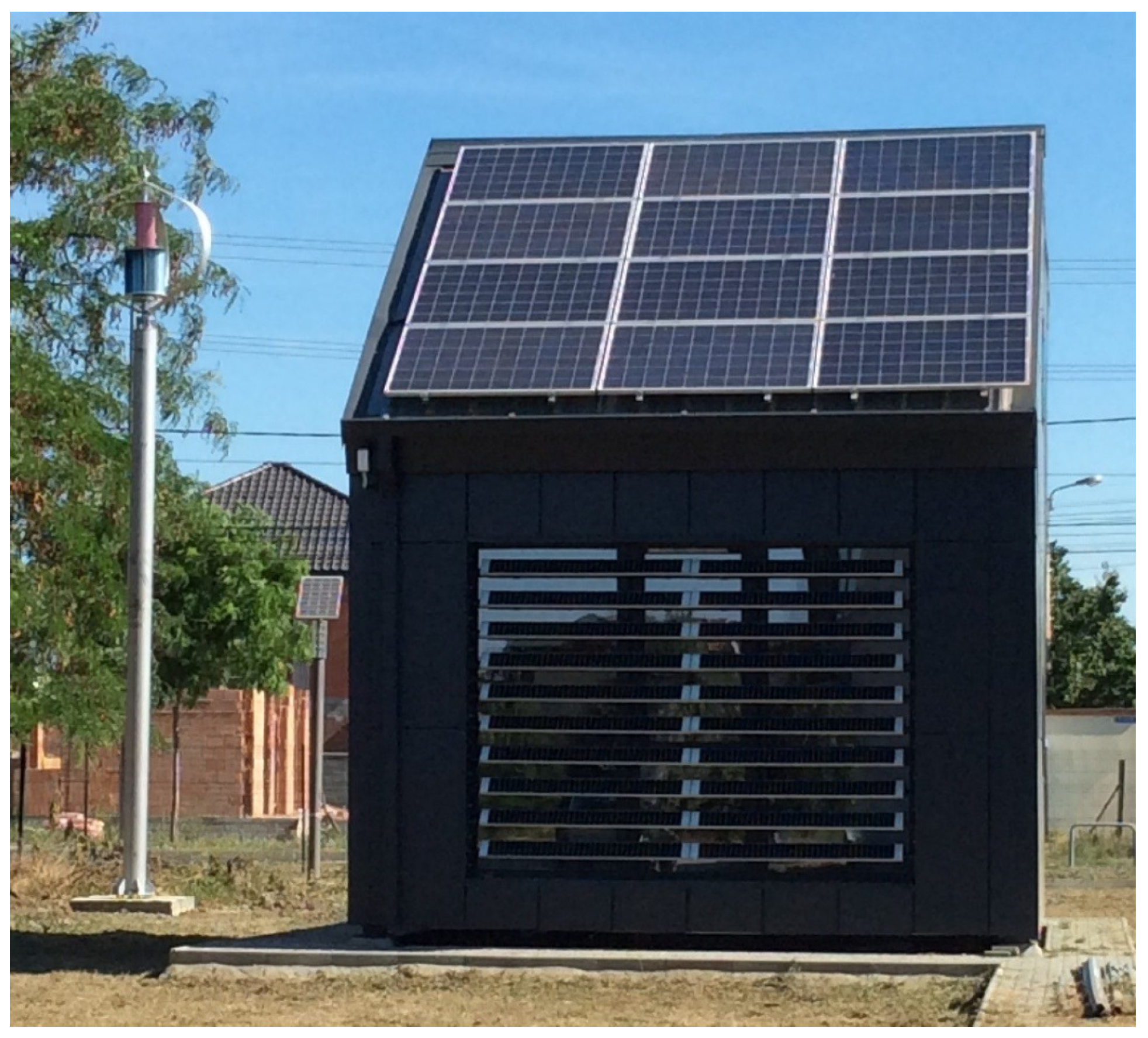
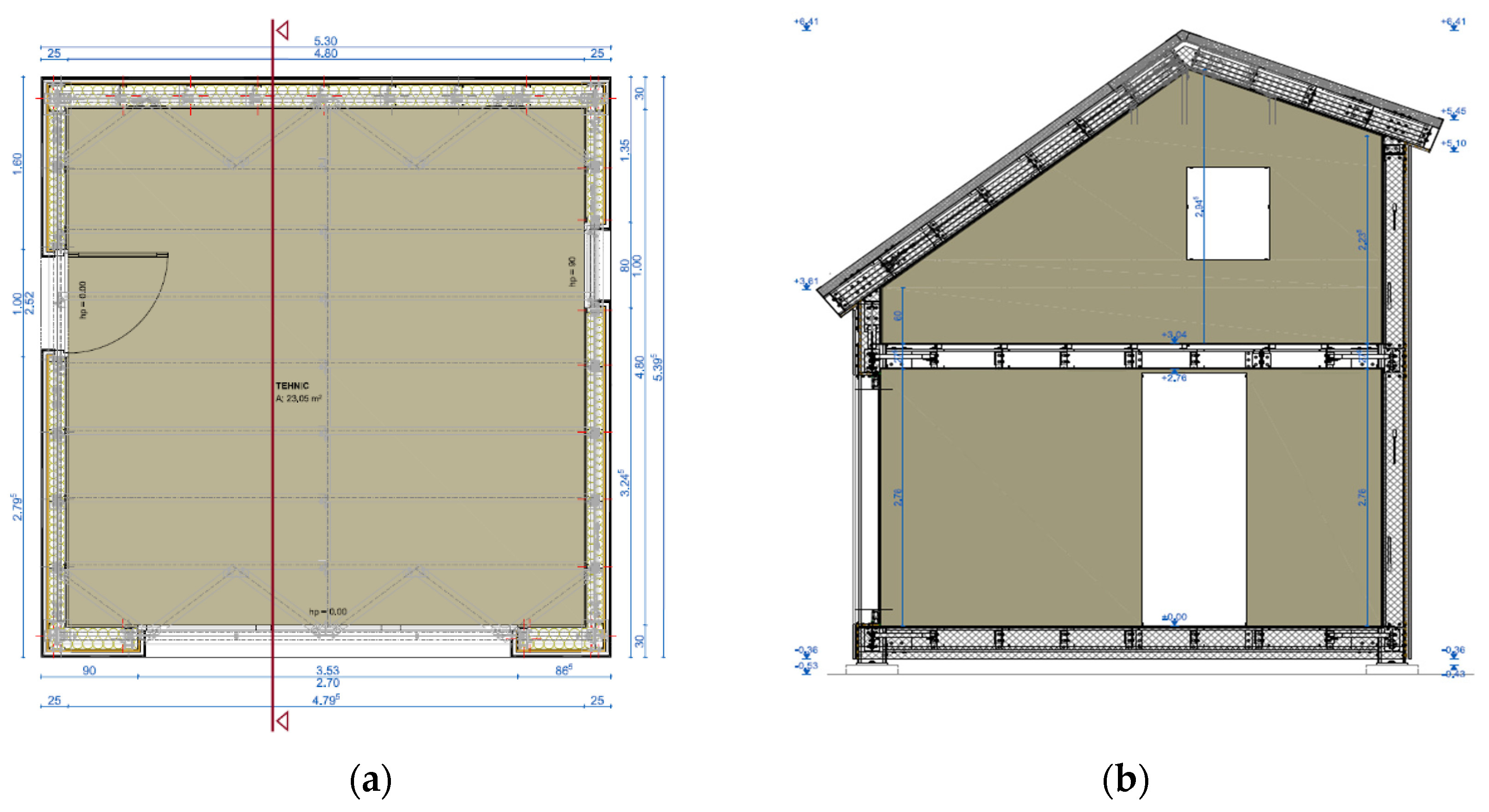
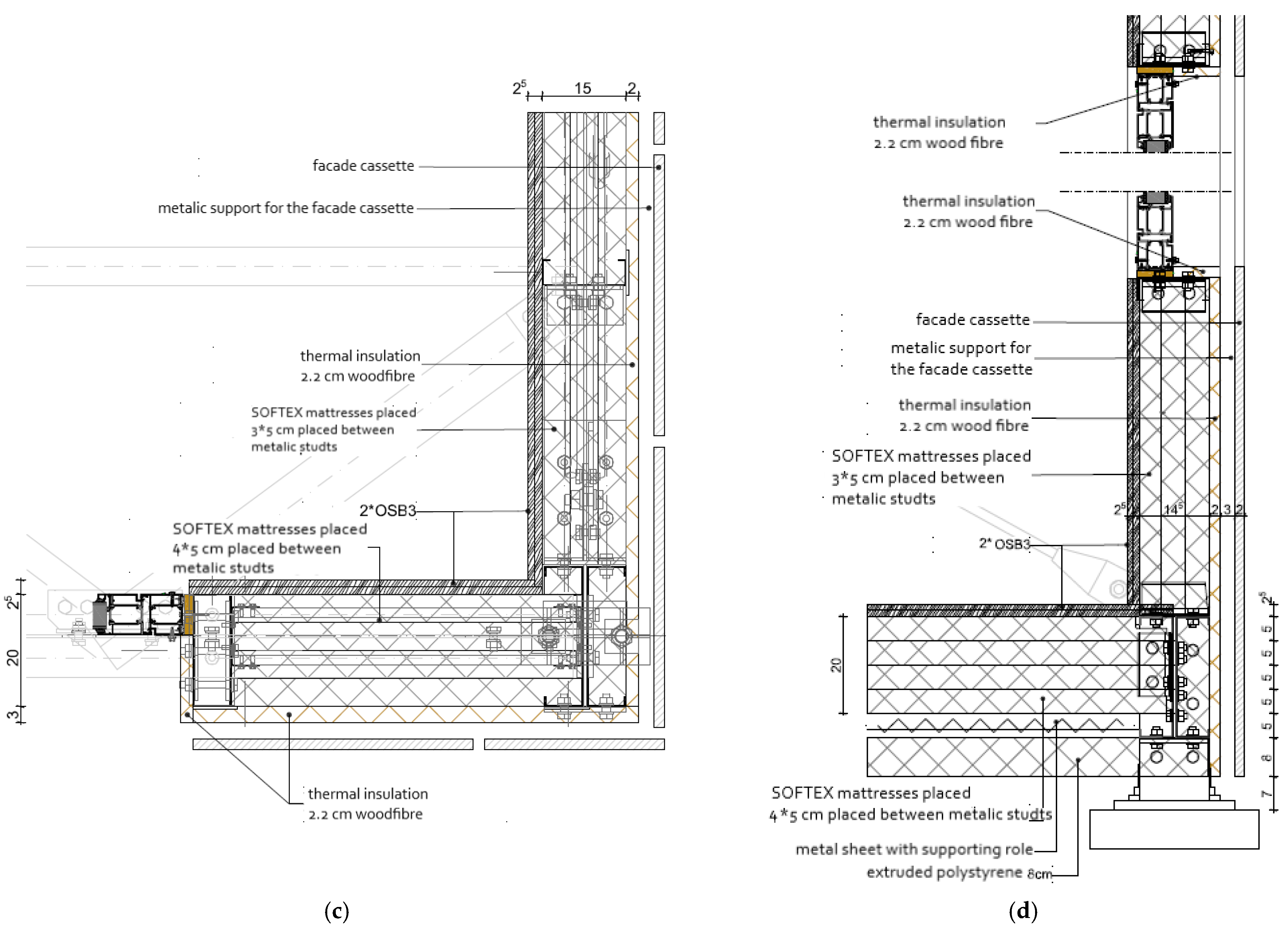
2.2. The Experimental Module
3. Materials and Methods
3.1. Numerical Approach
3.2. Modelled Cases
4. Results and Discussion
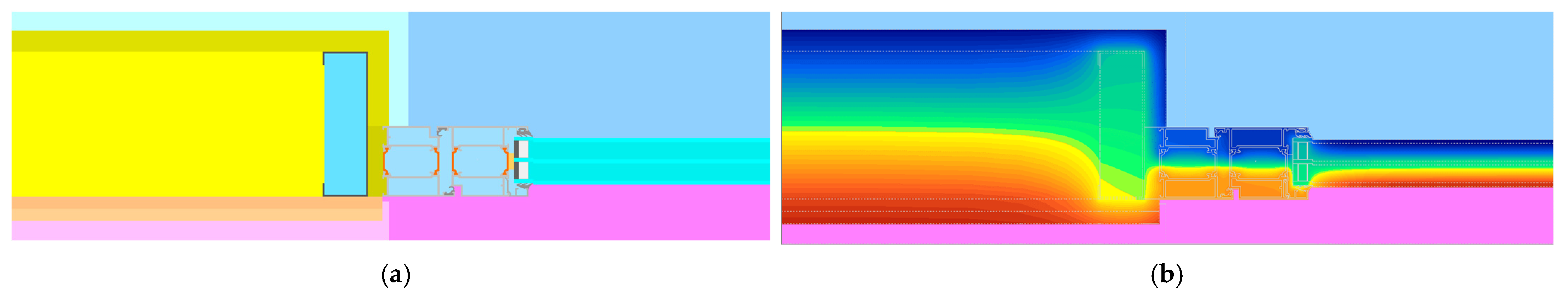
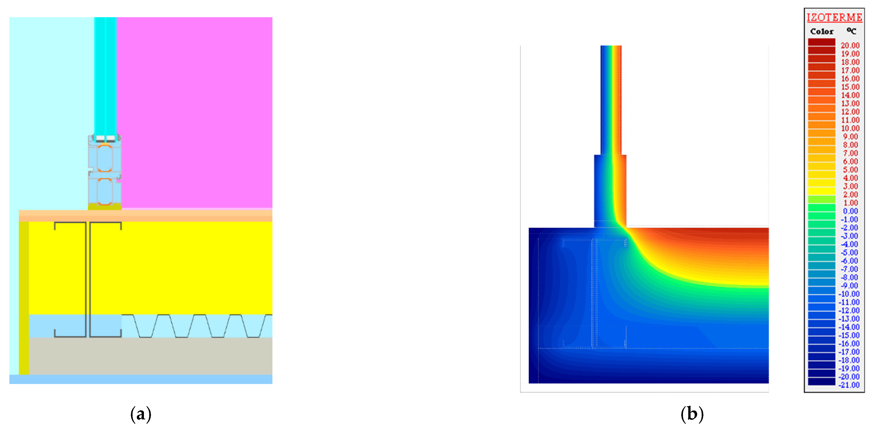
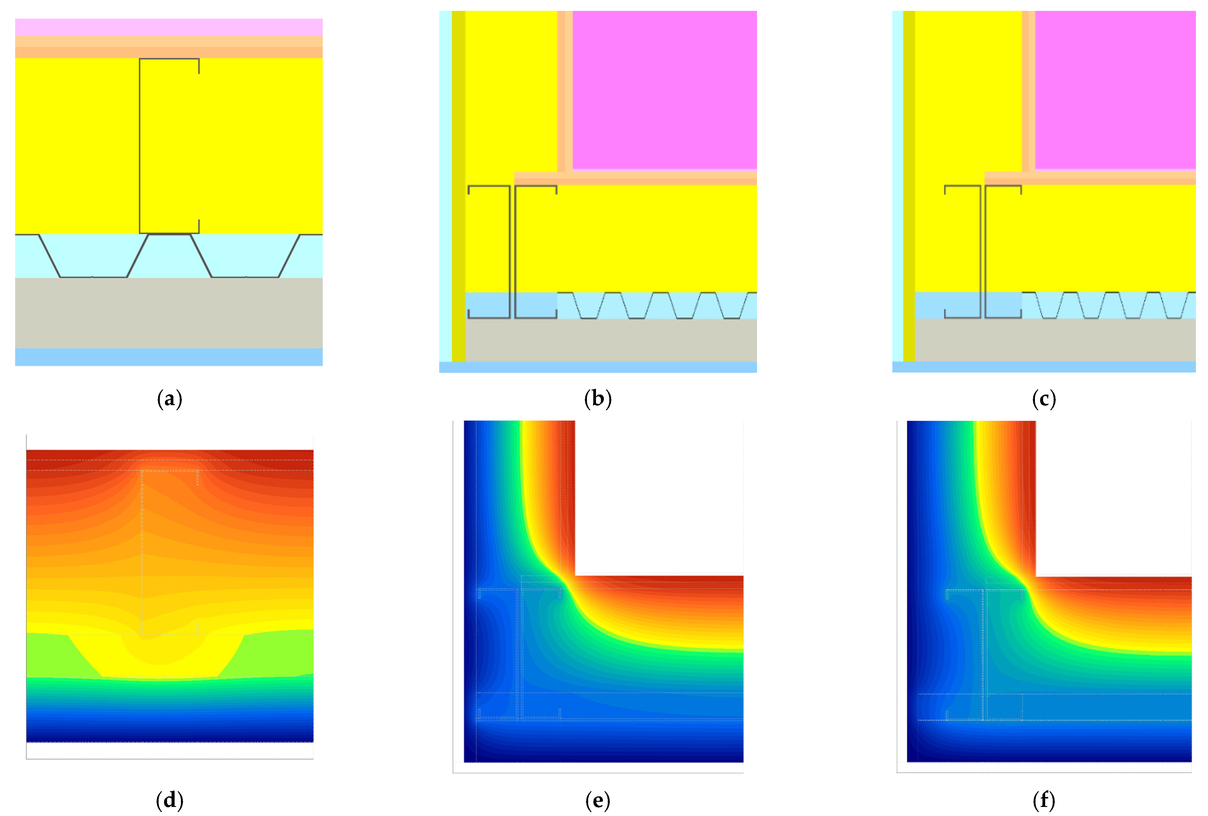
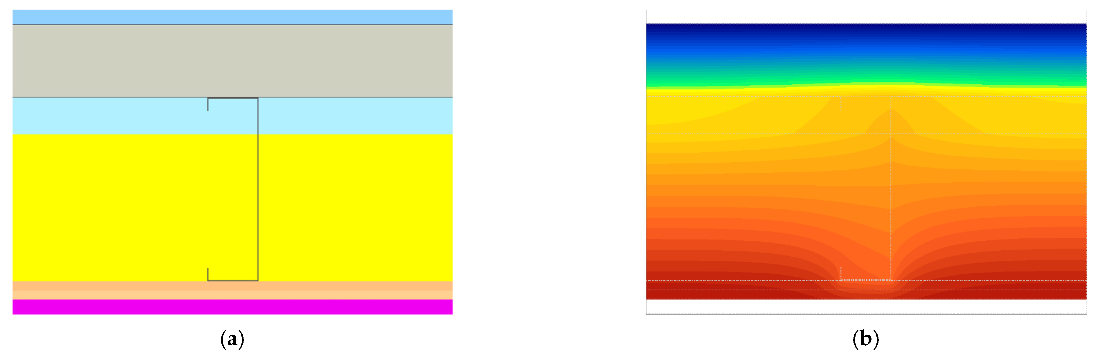
4.1. Thermal Performance per Element
4.2. Thermal Performance of the Building Envelope
4.3. Energy Performance for Heating of the Building
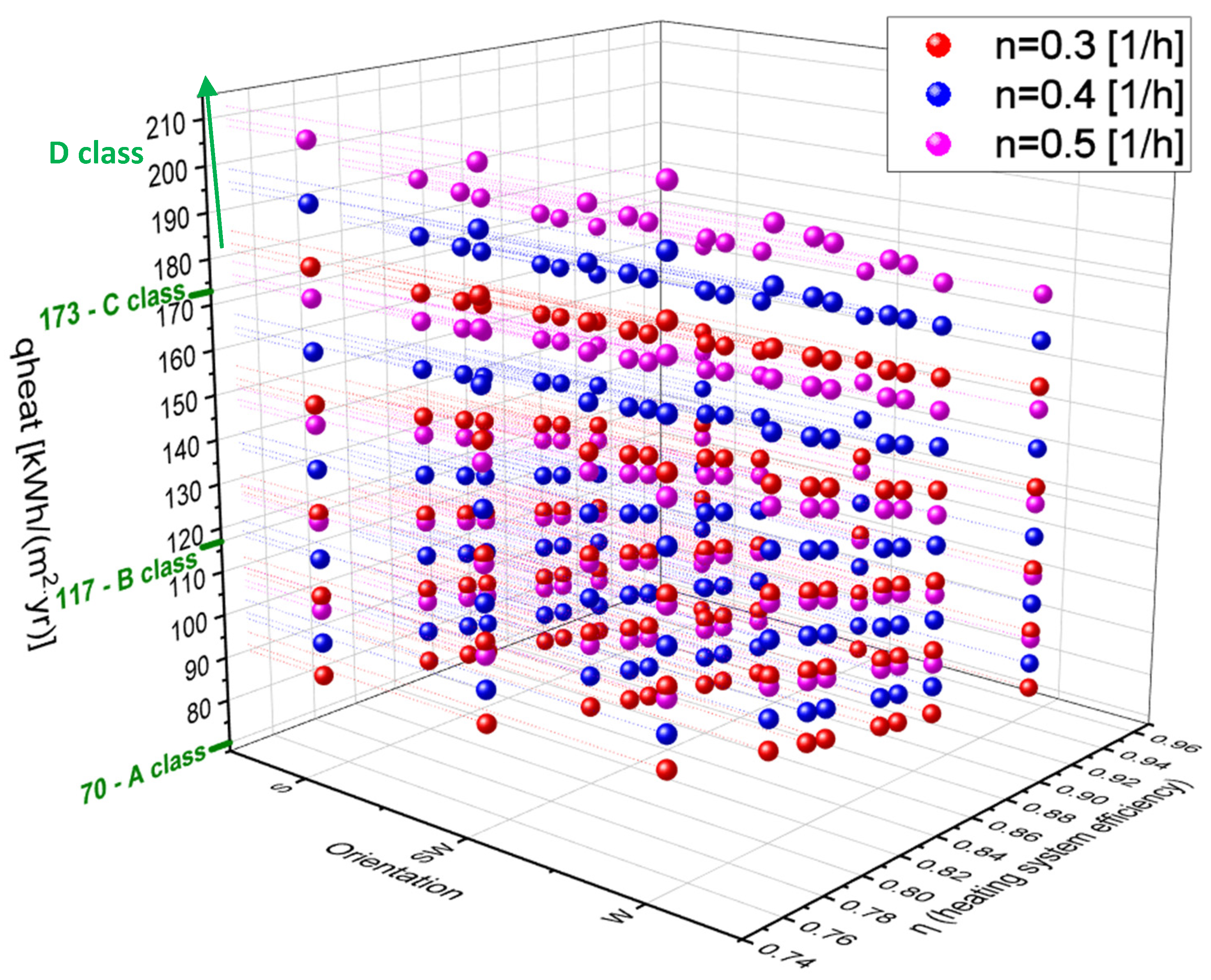
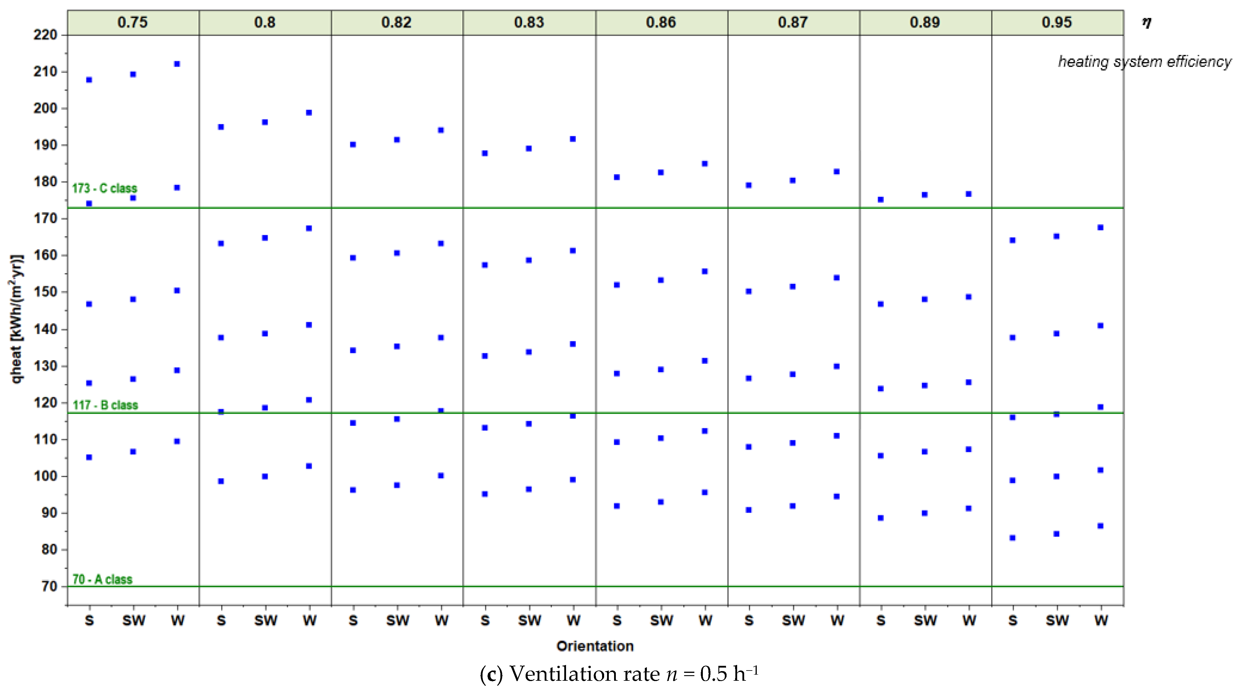
4.4. Parametric Study for the Energy Performance for Heating of the Building
4.5. Parametric Study for the Building Envelope Thermal Performance Impact on the Energy Consumption for Heating
5. Conclusions
Author Contributions
Funding
Institutional Review Board Statement
Informed Consent Statement
Data Availability Statement
Acknowledgments
Conflicts of Interest
Appendix A


References
- EU Commission. In Focus: Energy Efficiency in Buildings; EU Commission: Brussels, Belgium, 2020. [Google Scholar]
- EU Commission. A European Green Deal. Striving to be the First Climate-Neutral Continent; EU Commission: Brussels, Belgium, 2020. [Google Scholar]
- EU Commission. Directive (EU) 2018/844 of the European Parliament and of the Council of 30th May 2018 Amending Directive 2010/31/EU on the Energy Performance of Buildings and Directive 2012/27/EU on Energy Efficiency; EU Commission: Brussels, Belgium, 2018. [Google Scholar]
- EU Commission. National Energy and Climate Plans EU Countries’ 10-year National Energy and Climate Plans for 2021–2030; EU Commission: Brussels, Belgium, 2018. [Google Scholar]
- EU Commission. Directive 2012/27/EU of the European Parliament and of the Council of 25th October 2012 on Energy Efficiency, Amending Directives 2009/125/EC and 2010/30/EU and Repealing Directives 2004/8/EC and 2006/32/ECText with EEA Relevance; EU Commission: Brussels, Belgium, 2012. [Google Scholar]
- EU Commission. Proposal for a Directive of The European Parliament and of the Council on Energy Efficiency (Recast); EU Commission: Brussels, Belgium, 2021. [Google Scholar]
- EU Commission. ‘Fit for 55′: Delivering the EU’s 2030 Climate Target on the Way to Climate Neutrality; EU Commission: Brussels, Belgium, 2021. [Google Scholar]
- EU Commission. An EU-Wide Assessment of National Energy and Climate Plans Driving Forward the Green Transition and Promoting Economic Recovery through Integrated Energy and Climate Planning; EU Commission: Brussels, Belgium, 2020. [Google Scholar]
- International Energy Agency. Energy Efficiency 2019. The Authoritative Tracker of Global Energy Efficiency Trends. 2019. Available online: https://www.iea.org/reports/energy-efficiency-2019 (accessed on 14 October 2021).
- United Nations Environment Programme. 2020 Global Status Report for Buildings and Construction. Towards a Zero-Emissions, Efficient and Resilient Buildings and Construction Sector; United Nations Environment Programme: Nairobi, Kenya, 2020. [Google Scholar]
- Ürge-Vorsatz, D.; Cabeza, L.F.; Serrano, S.; Barreneche, C.; Petrichenko, K. Heating and cooling energy trends and drivers in buildings. Renew. Sustain. Energy Rev. 2015, 41, 85–98. [Google Scholar] [CrossRef] [Green Version]
- Romanian Ministry of Research and Innovation, CCCDI—UEFISCDI, project number PN-III-P1-1.2-PCCDI-2017-0391/CIA_CLIM–Smart Buildings Adaptable to the Climate Change Effects, within PNCDI III, 2018–2021. Available online: https://www.icer.ro/cercetare/proiecte-de-cercetare/cia-clim (accessed on 14 October 2021).
- Soares, N.; Santos, P.; Gervásio, H.; Costa, J.J.; Simões da Silva, L. Energy efficiency and thermal performance of lightweight steel-framed (LSF) construction: A review. Renew. Sustain. Energy Rev. 2017, 78, 194–209. [Google Scholar] [CrossRef]
- Santos, P.; Ribeiro, T. Thermal Performance Improvement of Double-Pane Lightweight Steel Framed Walls Using Thermal Break Strips and Reflective Foils. Energies 2021, 14, 6927. [Google Scholar] [CrossRef]
- Rajanayagam, H.; Upasiri, I.; Poologanathan, K.; Gatheeshgar, P.; Sherlock, P.; Konthesingha, C.; Nagaratnam, B.; Perera, D. Thermal Performance of LSF Wall Systems with Vacuum Insulation Panels. Buildings 2021, 11, 621. [Google Scholar] [CrossRef]
- Kempton, L.; Kokogiannakis, G.; Green, A.; Cooper, P. Evaluation of thermal bridging mitigation techniques and impact of calculation methods for lightweight steel frame external wall systems. J. Build. Eng. 2021, 43, 102893. [Google Scholar] [CrossRef]
- Santos, P.; Mateus, D. Experimental assessment of thermal break strips performance in load-bearing and non-load-bearing LSF walls. J. Build. Eng. 2020, 32, 101693. [Google Scholar] [CrossRef]
- Santos, P.; Lemes, G.; Mateus, D. Thermal Transmittance of Internal Partition and External Facade LSF Walls: A Parametric Study. Energies 2019, 12, 2671. [Google Scholar] [CrossRef] [Green Version]
- Ministry of Regional Development. Public Administration and European Funds, Order 2641 regarding the modification and completion of the technical regulation. In Methodology for Calculating the Energy Performance of Buildings; Approved by the Order of the Minister of Transport, Construction and Tourism no. 157/2007; Ministry of Regional Development: Bucharest, Romania, 2017. [Google Scholar]
- Ministry of Regional Development and Public Administration. Order 386 for the modification and completion of the Technical Regulation. In Normative Regarding the Thermotechnical Calculation of the Construction Elements of the Buildings; Indicative C 107-2005; Ministry of Regional Development and Public Administration: Bucharest, Romania, 2016. [Google Scholar]
- Ministry of Regional Development and Public Administration. Indicative Mc001 Part 6 Methodology for Calculating the Energy Performance of Buildings; Ministry of Regional Development and Public Administration: Bucharest, Romania, 2013. [Google Scholar]
- Buzatu, R.; Ungureanu, V.; Ciutina, A.; Gireadă, M.; Vitan, D.; Petran, I. Experimental Evaluation of Energy-Efficiency in a Holistically Designed Building. Energies 2021, 14, 5061. [Google Scholar] [CrossRef]
- Gorgolewski, M. Developing a simplified method of calculating U-values in light steel framing. Build. Environ. 2007, 42, 230–236. [Google Scholar] [CrossRef]
- Santos, P.; Gonçalves, M.; Martins, C.; Soares, N.; Costa, J.J. Thermal transmittance of lightweight steel framed walls: Experimental versus numerical and analytical approaches. J. Build. Eng. 2019, 25, 100776. [Google Scholar] [CrossRef]
- Ciutina, A.; Mirea, M.; Ciopec, A.; Ungureanu, V.; Buzatu, R.; Morovan, R. Behaviour of wedge foundations under axial compression. IOP Conf. Ser. Earth Environ. Sci. 2021, 664, 012036. [Google Scholar] [CrossRef]
- Buzatu, R.; Muntean, D.; Ciutina, A.; Ungureanu, V. Thermal Performance and Energy Efficiency of Lightweight Steel Buildings: A Case-Study. IOP Conf. Ser. Mater. Sci. Eng. 2020, 960, 032099. [Google Scholar] [CrossRef]
- Ciutina, A.; Buzatu, R.; Muntean, D.M.; Ungureanu, V. Heat transfer vs environmental impact of modern façade systems. E3S Web Conf. 2019, 111, 03078. [Google Scholar] [CrossRef] [Green Version]
- Intini, F.; Kühtz, S. Recycling in buildings: An LCA case study of a thermal insulation panel made of polyester fiber, recycled from post-consumer PET bottles. Int. J. Life Cycle Assess. 2011, 16, 306–315. [Google Scholar] [CrossRef]
- EN ISO 6946; European Committee for Standardization. Building Components and Building Elements—Thermal Resistance and thermal transmittance—Calculation Methods. CEN: Brussels, Belgium, 2017.
- de Angelis, E.; Serra, E. Light Steel-frame Walls: Thermal Insulation Performances and Thermal Bridges. Energy Procedia 2014, 45, 362–371. [Google Scholar] [CrossRef] [Green Version]
- C107 Norm for Thermotechnical Calculation of the Construction Elements of Buildings, Bucharest, Romania. 2005. Available online: https://ec.europa.eu/growth/tools-databases/tris/en/index.cfm/search/?trisaction=search.detail&year=2010&num=465&mLang=SV (accessed on 14 October 2021).
- Santos, P.; Poologanathan, K. The Importance of Stud Flanges Size and Shape on the Thermal Performance of Lightweight Steel Framed Walls. Sustainability 2021, 13, 3970. [Google Scholar] [CrossRef]
- Moga, L.; Moga, I. Considerations on the Thermal Modelling of Insulated Metal Panel Systems. In Proceedings of the International Building Physics Conference, Syracuse, NY, USA, 26 September 2018. [Google Scholar] [CrossRef]
- Lupan, L.; Manea, D.; Moga, L. Improving Thermal Performance of the Wall Panels Using Slotted Steel Stud Framing. Proc. Technol. 2016, 22, 351–357. [Google Scholar] [CrossRef] [Green Version]
- EN ISO 10211; European Committee for Standardization. Thermal Bridges in Building Construction—Heat Flows and Surface Temperatures—Detailed Calculations. CEN: Brussels, Belgium, 2017.
- PSIPLAN Software. Two-Dimensional Heat Transfer for Building Modelling Software for Calculating the Linear Thermal Transmittance Value; Technical University of Cluj-Napoca: Cluj-Napoca, Romania, 2021. [Google Scholar]
- Moga, L.; Moga, I. Evaluation of Thermal Bridges Using Online Simulation Software. E3S Web Conf. 2020, 172, 08010. [Google Scholar] [CrossRef]
- Moga, L. Analytic Study of Thermal Bridges Met at High Performance Energy Efficient Buildings. Inter. Multidis. Scien. GeoConf. SGEM 2018, 18, 621–626. [Google Scholar] [CrossRef]
- Moga, L.; Moga, I. Specific Thermal Bridges at Load Bearing Masonry Buildings; UTPRESS: Cluj-Napoca, Romania, 2013. [Google Scholar]
- ISO 13789; Thermal Performance of Buildings–Transmission and Ventilation Heat Transfer Coefficients—Calculation Method. ISO: Brussels, Belgium, 2015.
- ISO 52016-1; Energy Performance of Buildings—Energy Needs for Heating and Cooling, Internal Temperatures and Sensible and Latent Heat Loads—Part 1: Calculation Procedures. ISO: Brussels, Belgium, 2017.
- Ubakus—Online U-Wert Calculator. Available online: https://www.ubakus.de/u-wert-rechner/ (accessed on 5 October 2021).
- Ministry of Transportation. Constructions and Tourism, Indicative Mc001 Parts 1,2,3 Methodology for Calculating the Energy Performance of Buildings; Ministry of Transportation: Bucharest, Romania, 2006. [Google Scholar]
- Ministry of Development, Public Works and Administration Indicative Mc001 2021 Methodology for Calculating the Energy Performance of Buildings-Updated Version Preprint, Bucharest, Romania. Available online: https://epbd-ca.eu/ca-outcomes/outcomes-2015-2018/book-2018/countries/romania (accessed on 14 October 2021).
- Vajó, B.; Lakatos, Á. Super Insulation Materials—An Application to Historical Buildings. Buildings 2021, 11, 525. [Google Scholar] [CrossRef]
- Lakatos, Á. Thermophysical investigations of nanotechnological insulation materials. AIP Conf. Proc. 2017, 1866, 030003. [Google Scholar] [CrossRef] [Green Version]
- Lakatos, Á.; Csarnovics, I.; Csík, A. Systematic Analysis of Micro-Fiber Thermal Insulations from a Thermal Properties Point of View. Appl. Sci. 2021, 11, 4943. [Google Scholar] [CrossRef]
- ISO 13788; Hygrothermal Performance of Building Components and Building Elements—Internal Surface Temperature to Avoid Critical Surface Humidity and Interstitial Condensation—Calculation Methods. ISO: Brussels, Belgium, 2012.
- Șoimoșan, T.M.; Moga, L.M.; Anastasiu, L.; Manea, D.L.; Căzilă, A.; Zeljković, Č. Overall Efficiency of On-Site Production and Storage of Solar Thermal Energy. Sustainability 2021, 13, 1360. [Google Scholar] [CrossRef]
- Jack, R. Building Diagnostics: Practical Measurement of the Fabric Thermal Performance of House; Figure share; Loughborough University: Loughborough, UK, 2015. [Google Scholar]


| Material | Thermal Conductivity [W/(m∙K)] | Specific Heat [J/kg∙°C] | Density [kg/m3] |
|---|---|---|---|
| Steel profiles (C150/3, C200/3) | 50.00 | 420 | 7800 |
| OSB 1 | 0.130 | 1700 | 620 |
| Recycled-PET 2 thermal wadding | 0.054 | 1350 | 20 |
| Wood fibreboard | 0.050 | 2100 | 270 |
| Vapor barrier | 0.220 | 1700 | 130 |
| Aluminium sheet | 160.00 | 880 | 2800 |
| XPS 3 | 0.035 | 1450 | 35 |
| PIR 4 sandwich panel | 0.023 | 1400 | 30 |
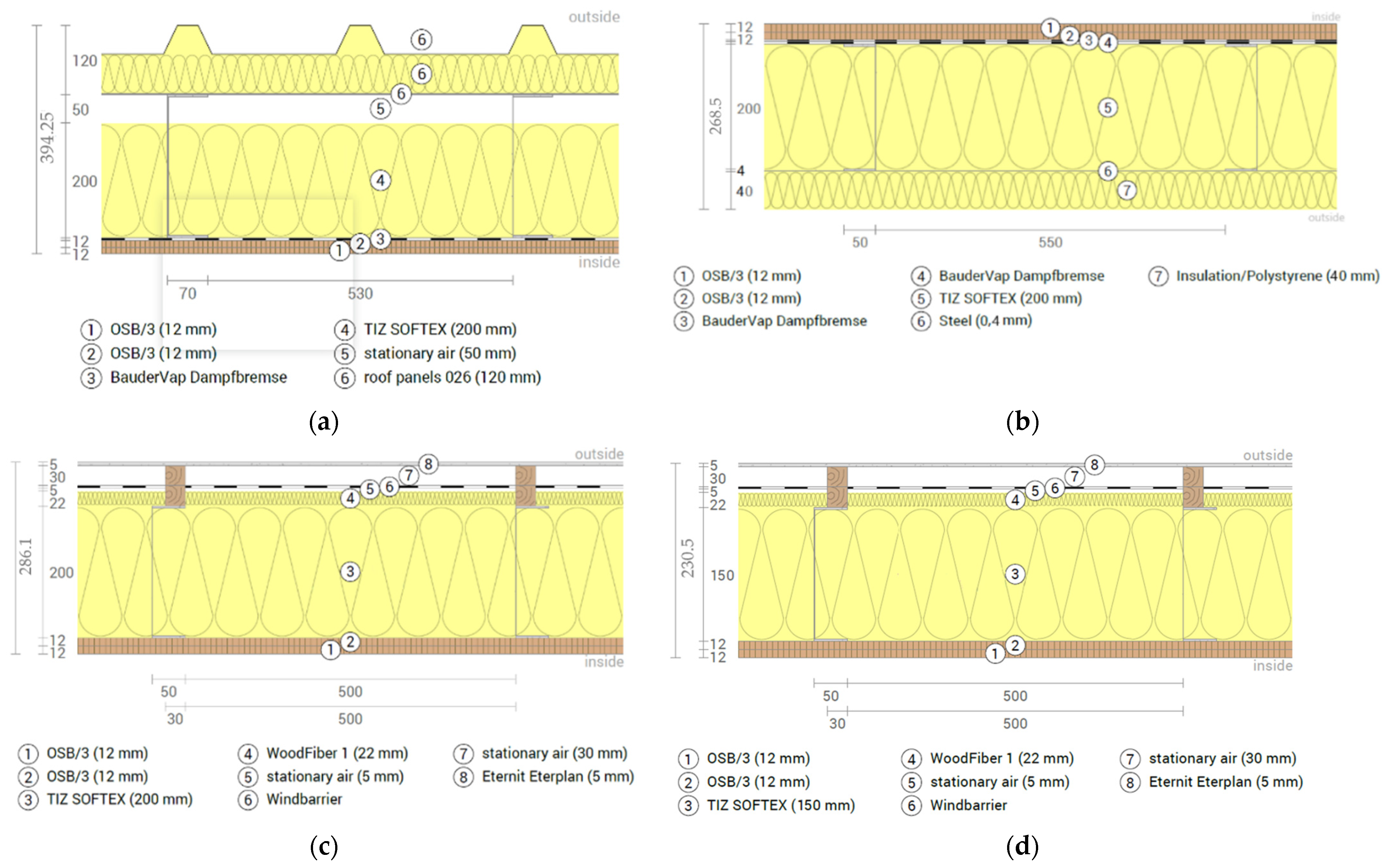
| Element | Material Layers (from Inside to Outside) | d [mm] | R′-Value [(m2·K)/W] | U′-Value [W/(m2·K)] |
|---|---|---|---|---|
| Ground floor above the crawl space | OSB | 24 | 3.677 | 0.272 |
| Recycled-PET thermal wadding TIZ SOFTEX | 200 | |||
| Steel sheet | 4 | |||
| XPS | 40 | |||
| Total thickness | 268.5 | |||
| Exterior walls (north) | OSB | 24 | 3.185 | 0.314 |
| Recycled-PET thermal wadding-TIZ SOFTEX | 200 | |||
| Wood fibreboard | 22 | |||
| Stationary air | 5 | |||
| Wind barrier | ||||
| Rear ventilated level (outside air) | 30 | |||
| Fiber cement plate | 5 | |||
| Total thickness | 286.1 | |||
| Exterior walls (east and west) | OSB | 24 | 2.817 | 0.355 |
| Recycled-PET thermal wadding TIZ SOFTEX | 150 | |||
| Wood fibreboard | 22 | |||
| Stationary air | 5 | |||
| Wind barrier | ||||
| Rear ventilated level (outside air) | 30 | |||
| Fiber cement plate | 5 | |||
| Total thickness | 230.5 | |||
| Roof | OSB | 24 | 5.208 | 0.192 |
| Recycled-PET thermal wadding TIZ SOFTEX | 200 | |||
| Stationary air | 50 | |||
| PIR sandwich panel | 120 | |||
| Total thickness | 394.25 | |||
| Door and windows | Glass with argon filling | 24 | 1.136 | 0.880 |
| PVC casement | 92 | |||
| Glass Curtain | Glass with argon filling | 44 | 1.351 | 0.740 |
| PVC casement | 92 |
| Modelled Cases | Rtot-Value [(m2∙K)/W] | R′-Value [(m2∙K)/W] | U′-Value [W/(m2∙K)] | ψ-Value [W/(m∙K)] | fRsi-Value [-] |
|---|---|---|---|---|---|
| Exterior wall current field (east and west) | 3.660 | 2.637 | 0.379 | 0.066 | 0.802 |
| Exterior walls current field (north) | 4.586 | 2.981 | 0.335 | 0.073 | 0.823 |
| Exterior corner | 4.071 | 2.059 | 0.486 | 0.120 | 0.690 |
| South Exterior wall-curtain wall left margin | 4.586 | 1.748 | 0.572 | 0.136 | 0.827 |
| South Exterior wall-curtain wall right margin | 4.586 | 1.6542 | 0.218 | 0.148 | 0.826 |
| Exterior wall-window | 3.660 | 1.841 | 0.543 | 0.104 | 0.796 |
| Curtain glass—Ground floor above the crawl space | 2.053 | 1.714 | 0.583 | 0.072 | 0.748 |
| Exterior wall (E,W)—Ground floor above the crawl space | 4.584 | 2.817 | 0.355 | 0.082 | 0.807 |
| Exterior wall (N)—Ground floor above the crawl space | 5.247 | 3.140 | 0.319 | 0.077 | 0.822 |
| Ground floor above the crawl space—current field | 6.453 | 3.951 | 0.253 | 0.034 | 0.918 |
| Exterior wall (E,W)—intermediate floor | 3.660 | 2.476 | 0.404 | 0.101 | 0.922 |
| Exterior wall (N)—intermediate floor | 4.586 | 3.454 | 0.290 | 0.055 | 0.945 |
| Roof—current field | 7.987 | 5.924 | 0.169 | 0.0216 | 0.953 |
| Roof ridge | 7.987 | 3.981 | 0.251 | 0.086 | 0.943 |
| Roof eaves—exterior wall | 5.621 | 2.845 | 0.351 | 0.170 | 0.938 |
| Modelled Cases | Subdivisions | Rtot-Value [(m2∙K)/W] | R′-Value [(m2∙K)/W] | U′-Value [W/(m2∙K)] | ψ-Value [W/(m∙K)] | fRsi-Value [-] |
|---|---|---|---|---|---|---|
| Curtain glass—Ground floor above the crawl space | Curtain glass wall | 1.351 | 1.384 | 0.723 | −0.007 | 0.748 |
| Ground floor above the crawl space | 6.132 | 2.467 | 0.405 | 0.079 | 0.636 | |
| Exterior wall (E,W)—Ground floor above the crawl space | Exterior wall (E,W) | 3.660 | 2.510 | 0.398 | 0.038 | 0.807 |
| Ground floor above the crawl space | 6.132 | 3.211 | 0.311 | 0.045 | 0.777 | |
| Exterior wall (N)—Ground floor above the crawl space | Exterior wall (N) | 4.586 | 2.897 | 0.345 | 0.038 | 0.794 |
| Ground floor above the crawl space | 6.132 | 3.426 | 0.292 | 0.039 | 0.822 | |
| Roof eaves—exterior wall | Roof eaves | 7.987 | 2.510 | 0.398 | 0.116 | 0.895 |
| Exterior wall | 4.586 | 3.167 | 0.316 | 0.054 | 0.938 |
| Type | Building Envelope Element | ATotal | R′ | |
|---|---|---|---|---|
| [m2] | [m2 K/W] | [W/K] | ||
| 1 | Exterior Wall | 76.57 | 2.36 | 32.49 |
| 2 | Roof | 27.61 | 3.86 | 7.15 |
| 3 | Ground floor above the crawl space | 23.04 | 3.30 | 6.99 |
| 4 | Curtain wall | 9.53 | 1.35 | 7.06 |
| 5 | Glazing surfaces | 4.92 | 1.14 | 4.33 |
| Building Envelope | ATotal | R′m | U′m | |
|---|---|---|---|---|
| [m2] | [m2 K/W] | [W/K] | [W/m2 K] | |
| Total B. Env. | 141.67 | 2.69 | 58.02 | 0.37 |
| Parameters | Examined Range |
|---|---|
| Climatic zone | 1st, 2nd, 3rd, 4th and 5th zone |
| Curtain wall orientation | S, SW, W |
| Ventilation rate, n [h−1] | 0.5, 0.4, 0.3 |
| Heating system efficiency, η [%] | 75—Hot-water floor heating system 40°/30 °C 80—Water radiator 70°/40 °C with manifold 82—Electric floor heating 83—Water radiator 45°/35 °C with manifold 86—Roof heating (i.e., electric) 87—Water radiator 70°/40 °C 89—Water radiator 45°/35 °C 95—Electric heater |
| Values | qheat [kWh/(m2·yr)]—Energy Class per Climatic Zone | ||||
|---|---|---|---|---|---|
| 1st | 2nd | 3rd | 4th | 5th | |
| Minimum | 71.09—B | 85.46—B | 100.17—B | 119.21—C | 142.77—C |
| Maximum | 109.38—B | 128.62—B | 150.37—C | 178.40—C | 211.99—D |
| Type | Building Envelope Element | R′ [m2 K/W] | ||||
|---|---|---|---|---|---|---|
| Ref. | (1) | (2) | (3) | (4) | ||
| 1 | Exterior Wall | 2.36 | 2.36 | 2.36 | 2.36 | 4.00 |
| 2 | Roof | 3.86 | 5.00 | 3.86 | 5.00 | 6.67 |
| 3 | Ground floor above the crawl space | 3.30 | 3.30 | 4.50 | 4.50 | 5.00 |
| 4 | Curtain wall | 1.35 | 1.35 | 1.35 | 1.35 | 1.35 |
| 5 | Glazing surfaces | 1.14 | 1.14 | 1.14 | 1.14 | 1.14 |
| qheat [kWh/(m2·yr)] | 107.79 | 104.70 | 104.25 | 101.14 | 72.12 | |
| Reduction | 3% | 3% | 6% | 33% | ||
Publisher’s Note: MDPI stays neutral with regard to jurisdictional claims in published maps and institutional affiliations. |
© 2022 by the authors. Licensee MDPI, Basel, Switzerland. This article is an open access article distributed under the terms and conditions of the Creative Commons Attribution (CC BY) license (https://creativecommons.org/licenses/by/4.0/).
Share and Cite
Moga, L.; Petran, I.; Santos, P.; Ungureanu, V. Thermo-Energy Performance of Lightweight Steel Framed Constructions: A Case Study. Buildings 2022, 12, 321. https://doi.org/10.3390/buildings12030321
Moga L, Petran I, Santos P, Ungureanu V. Thermo-Energy Performance of Lightweight Steel Framed Constructions: A Case Study. Buildings. 2022; 12(3):321. https://doi.org/10.3390/buildings12030321
Chicago/Turabian StyleMoga, Ligia, Ioan Petran, Paulo Santos, and Viorel Ungureanu. 2022. "Thermo-Energy Performance of Lightweight Steel Framed Constructions: A Case Study" Buildings 12, no. 3: 321. https://doi.org/10.3390/buildings12030321