The Relationship between Wind Pressure and Pressure Coefficients for the Definition of Wind Loads on Buildings

Abstract

Wind induced pressures on buildings are the product of a velocity pressure and a pressure coefficient. The way in which these two quantities are calculated has changed over the years, and Design Codes have been modified accordingly. This paper tracks the evolution of the approach to wind loading of buildings from the practice in the 1950s, mainly referring to the Swiss Code SIA, to the most recent advances including probabilistic methods, internet databases, and advanced modelling of meteorological phenomena.

1. Introduction

Broadly speaking, the action exerted by the wind on a body is proportional to the wind velocity pressure through an aerodynamic coefficient, accounting for the way in which the body interacts with the flow. In the ideal case in which the flow is laminar and the body is streamlined, the surface pressure can be expressed as:

$$w=q·c$$

(1)

where $q=0.5\rho v^2$ is the velocity pressure, and $c=c\left(M\right)$ is the pressure coefficient, depending on the location M where pressure is measured. This is not quite the case for Civil construction in general and for buildings in particular. Indeed, wind in the low atmosphere is characterized by a turbulent boundary layer flow, in which the mean wind speed is variable with the height above the ground, and to which a three-component turbulence is superimposed. In addition, civil constructions quite seldom meet the requirement of a streamlined shape, being instead bluff bodies. The bluff shape causes flow separation, generating additional turbulence to the oncoming one, the so-called signature turbulence, whose characteristics are related to the aerodynamics of the building and to a lesser extent to the characteristics of the oncoming wind. Finally, the mean and fluctuating properties of the wind flow cannot be defined through a deterministic approach, but rather need a probabilistic treatment. Combination of the three aspects above makes Equation (1) the general expression of a physical law, yet unable to alone give a quantitative definition of the load.

The structure of Equation (1) seems to separate well that which derives from the characteristics of the flow from the effects of aerodynamics, yet this separation is not unique, and lends itself to many possible interpretations, as well as to potential misunderstandings. In fact, the meaning of the two terms appearing to the hand right side of the equation must be properly defined from both the physical and the statistical points of view.

In this paper, the evolution of Equation (1) from its first use to modern applications is briefly outlined. For use of designers making their way through Codes of Practice, the meaning and use of Code equations are also explained.

2. Early Studies on Building Aerodynamics

With the aim of experimentally measuring wind loads on simple objects, in 1871 the first wind tunnel was built by F. H. Wenham. The results of his tests on flat inclined plates were then used by W. Unwin, who first attempted to evaluate wind pressures on building roof surfaces [1]. In doing this, a first major error arose, that of assuming that the load measured on an isolated element remains the same when the element becomes part of an assemblage; this is not quite true, as the pressure distribution is related to the overall geometry, and not merely of that of the detail where it is measured. The first wind tunnel for civil engineering applications was built in 1890 in Melbourne, Australia, by W. C. Kernot with the purpose of measuring wind pressures on a flat plate orthogonal to the flow. In the coming years, wind tunnels were built also in Denmark by J. O. V. Irminger (1893) and in France by A. G. Eiffel (1909), both aimed at assessing wind loads on civil structures. Aerodynamic studies began to develop rapidly, and the first heavier-than-air flight was achieved in 1903, making aerodynamics the crucial issue in the development of aeronautics. For more than 50 years civil and aeronautical aerodynamics, though differing from each other, were investigated in the same experimental facilities as it had not yet been recognized that the flow encountered by aircraft flying at hundreds or thousands of meters of height is quite different from that hitting ground-based Civil constructions. This misunderstanding is at the base of perhaps the major mistake made in earlier times when evaluating wind loads on Civil structures.

In the early 1900s, the need for specific studies on the pressures exerted by the wind on buildings began to arise. Until the 1950s, the pressure distribution on plates with different shapes, dimensions and pitch angles were investigated in wind tunnels, and the results were used to evaluate the loading of the upwind surfaces of building. Only later, the important role of suction on the leeward surfaces when evaluating the overall forces due to wind was acknowledged [2,3,4]. [2] first carried out several experiments on rectangular model buildings with sloped roofs, showing the pressure pattern along the middle section of the tested models. Then, Irminger and Nøkkentved [5], Irminger and Nøkkentved [6] used flow visualization to show that (i) the upwind face was subject to (over)pressure; that (ii) the leeward and side faces, as well as the downwind roof slope were subject to negative pressure (or suction); and that (iii) the upwind slope was exposed to either positive or negative pressures depending on its inclination. Moreover, the dependency of the pressure distribution on the ratio between width, depth, and height of the building was also highlighted. In their experiments, Irminger and Nøkkentved [5,6] and Nøkkentved [7] acknowledged the role of the wind tunnel floor roughness in influencing the wind speed profile and thus affecting the distribution and the intensity of wind pressures on model buildings.

In the meantime, starting from 1928 the first regulations on building design due to wind loading were introduced in Europe. More or less at the same time, on the US the American Society of Civil Engineering (ASCE) started working at recommendation for ’Wind Bracing in Steel Buildings’, incorporating all the available data and studies [8]. The values of the pressure coefficients were based on a collection of measurements made in wind tunnels with smooth flow conditions, and on models often detached from the tunnel floor; therefore, despite the detailed description of the pressure pattern they provide, such measurement are now known to be useless as wrong.

The first attempt to compare wind tunnel measurements with full-scale data was made by Bailey [9], showing quantitative differences between the results coming from the two approaches. Based on the work of Nøkkentved [7], Bailey and Vincent [10] made one of the first experiments in a boundary layer wind tunnel, simulating the flow in the low atmosphere, finding good agreement with full-scale measurements. The turning point in the assessment of wind pressures on buildings was the work of Jensen in 1950s. Continuing the work of Nøkkentved, Jensen [11] clarified the role of ground roughness in generating wind turbulence, and first pointed out the need and set the rules for properly scaling the atmospheric boundary layer in the wind tunnel. Jensen’s model law states that the ratio $h/z_{\mathrm{o}}$ (also known as Jensen Number, $Je$) between the building height, h, and the roughness length, $z_{\mathrm{o}}$, should be the same in wind tunnel as it is in full scale. Despite the work of Jensen, it took many years before that tests in boundary layer wind tunnel became commonly available, and in 1956 one of the first wind Codes (SIA 160) was published in Switzerland, still incorporating pressure and force coefficients measured in smooth flow [12].

3. The Modern Wind Engineering Approach

Besides the error in modelling the flow in the wind tunnel, until the 1960s the assessment of wind loads was based on the wrong hypothesis of steady wind resulting in steady pressures. This is now known not to be true, especially even in the case of bluff geometries causing flow separation, therefore a fluctuating separated shear layer and a turbulent wake. These aerodynamic features produce surface pressure fluctuations on the body, even when the flow in which this is immersed is laminar; broadly speaking, the wind velocity fluctuations induced by separation are referred to as signature turbulence. Before the spread of the use of Extreme Value statistics, Equation (1) was meant as the combination of the largest value of the velocity pressure at the site (often coinciding with the largest value ever measured, clearly depending on the measuring technique, on the length of the observation window, as well as on the inherent randomness of the quantity) and an average value of the pressure coefficient. This, of course, led to neglecting both the oncoming and signature turbulence.

In the 1960s, the various aspects of the wind loading of structures were integrated together into a comprehensive theory by Davenport [13], setting the stage for the Alan G. Davenport Wind Loading Chain [14,15], and starting the era of modern Wind Engineering. In this process played their role the use of boundary layer wind tunnels and the establishment of a series of International Conferences on Wind Effects on Buildings and Structures (now International Conference on Wind Engineering, ICWE) allowing the exchange of ideas and research results.

Davenport [16] first observed the need for a statistical approach to wind loading, introducing the concept of ”basic design wind speed”, defined as an ”extreme value statistics of the wind speed averaged over a minute”. In this definition, two notions were introduced: (1) the need for defining an averaging period for wind speeds, and nor rather considering instantaneous values; the latter, in fact, are not only affected by the measuring technique, but do not necessarily produce extreme effects on the structure, if their duration is too short; (2) the need for an Extreme Value (EV) analysis to evaluate the return wind speed, i.e., a fractile of the yearly maxima associated with a specified probability of exceedance. The choice of one minute as averaging period was justified by the wrong assumption that the average size of turbulent eddies was between $1.2$ and $1.8\mathrm{km}$, corresponding to a time scale of $60\mathrm{s}$ when the wind speed is $20\mathrm{m}/\mathrm{s}$ and $30\mathrm{m}/\mathrm{s}$, respectively; therefore averaging over a minute would have cancelled the turbulent fluctuations out. This is now known not to be true, as values in the order of 50 to $300\mathrm{m}$ apply to the turbulence scale during synoptic storms. However, more than that, what was lacking in the first work of Davenport was an appropriate treatment of the effects of turbulence on the wind loads.

Later, Davenport [13] better recognized the structure of the atmospheric turbulence and its impact on the wind loading. He proposed that the instantaneous wind speed is represented as the sum of a mean wind speed U averaged over a longer period, T, and a zero-mean turbulent component $u^{\prime }\left(t\right)$, averaged over a shorter period, $\tau$:

$$V\left(t\right)=U+u^{\prime }\left(t\right)=U·\left[1+{\displaystyle \frac{u^{\prime }\left(t\right)}{U}}\right]$$

(2)

In so doing, the peak wind speed is represented as the product of the mean wind speed and a gust factor $G_u$:

$$\widehat{V}=U·\left[1+g_u{I}_u\right]=U·G_u$$

(3)

where $I_u={\sigma }_u/U$ is the turbulence intensity, and $g_u$ is the velocity peak factor, indicating the average number of standard deviations ${\sigma }_u$ the peak wind speed exceeds the mean value. The peak factor was found to be a function of the averaging period and of the average rate ${\nu }_u$ at which the instantaneous speed up-crosses the mean value; when the turbulent fluctuations can be approximated by a Gaussian process:

$$g_u=\sqrt{2log\left({\nu }_{u}T\right)}+{\displaystyle \frac{0.5772}{\sqrt{2log\left({\nu }_{u}T\right)}}}$$

(4)

Based on the available measurements of the spectrum of the atmospheric turbulence, it is found that $g_u$ ranges between 2.8 and 2.9.

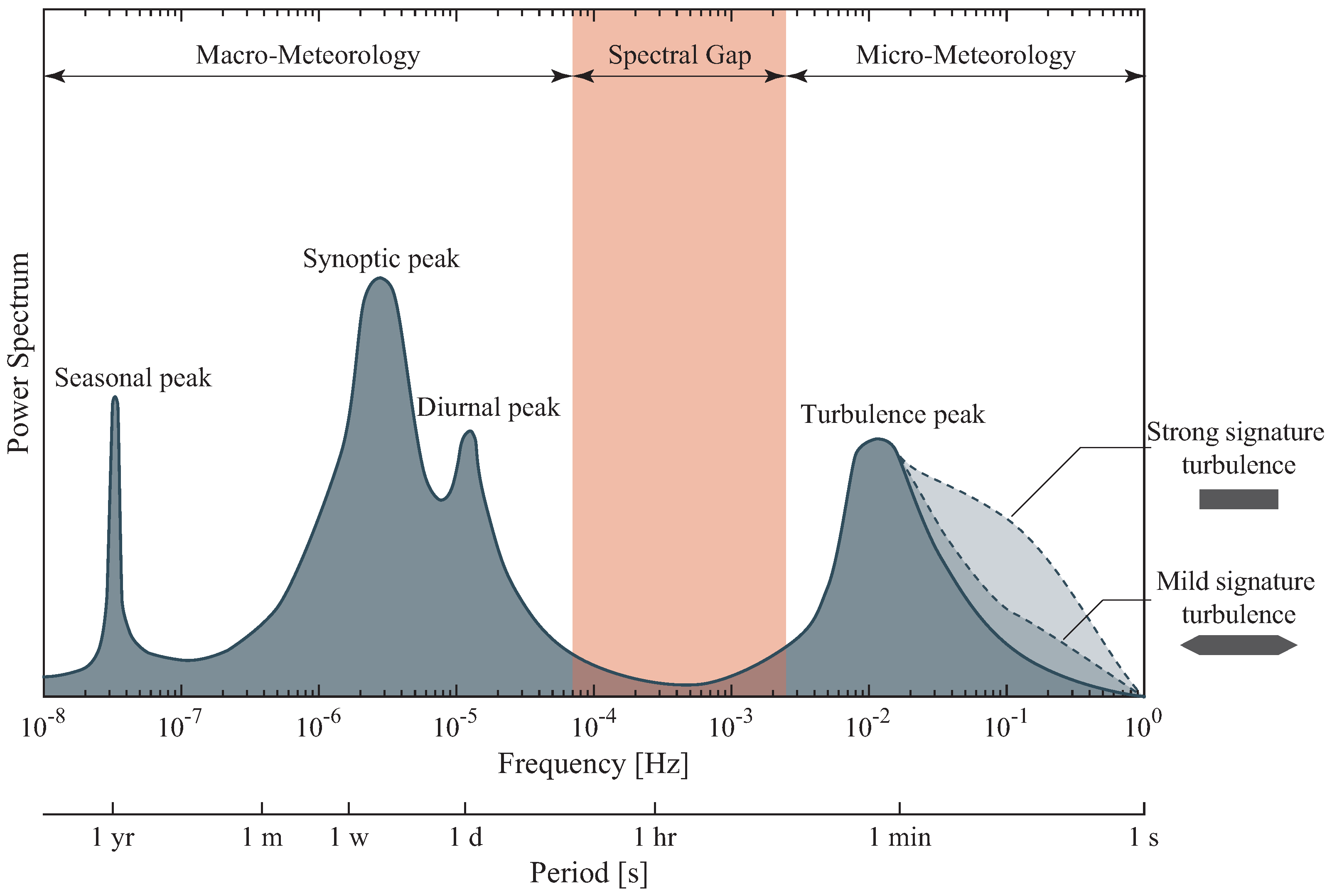
This procedure implies the choice of the averaging period and of the duration of the gust. Based on the Van der Hoven spectrum of the horizontal wind speed [17], Davenport [14] found it appropriate to use an averaging period of 1 h, accounting for the macro-meteorological fluctuations, and a duration of the gust of $3\mathrm{s}$, accounting for micro-meteorological fluctuations. In doing so, the mean wind speed was to be meant as the driving statistical quantity, to be evaluated by applying EV analysis to site-specific meteorological data, and the gust factor was to incorporate all the effects coming from ground surface roughness.

Applying the quasi-steady theory, i.e., assuming that the instantaneous value of the surface pressure in turbulent flow coincides with what it would be if the flow were laminar and the wind speed equal to the instantaneous turbulent speed, the instantaneous surface pressure at a point on the building is given by:

$$w\left(t\right)=0.5\rho V^2\left(t\right)·{\overline{c}}_p=0.5\rho U^2·{\left[1+{\displaystyle \frac{u^{\prime }\left(t\right)}{U}}\right]}^2·{\overline{c}}_p$$

(5)

where ${\overline{c}}_p$ is to be meant as the mean value of the measured pressure coefficient. Upon linearization of Equation (5), one obtains:

$$w\left(t\right)\simeq 0.5\rho U^2·\left[1+2{\displaystyle \frac{u^{\prime }\left(t\right)}{U}}\right]·{\overline{c}}_p$$

(6)

and the corresponding peak surface pressure $\widehat{w}$ is:

$${\widehat{w}}_{lin}={\overline{w}}_{lin}·\left[1+2g_u{I}_u\right]={\overline{w}}_{lin}·G_{w,lin}$$

(7)

where ${\overline{w}}_{lin}=0.5\rho U^2·{\overline{c}}_p$ and where $G_{w,lin}$ is a linearized gust loading factor, transforming the mean load into a peak load.

The linearization in Equation (6) is based on the assumption of small turbulence, i.e., that $u^{\prime }\left(t\right)\ll U$, and brings two major simplifications: first, the mean surface pressure coincides with the surface pressure associated with the mean wind speed; second, the fluctuating surface pressure is proportional to the turbulent component, $w_{lin}^{\prime }\left(t\right)\propto u^{\prime }\left(t\right)$ and ${\tilde{w}}_{lin}=2I_u{\overline{w}}_{lin}$. This latter assumption allows expressing the spectrum of the surface pressure fluctuations directly from the spectrum of the atmospheric turbulence: $S_w\propto S_{u^{\prime }}$. In case of high turbulence, linearization cannot be considered acceptable any more, and this makes all further steps much more complicated. From Equation (5), the mean surface pressure turns out to be:

$$\overline{w}=0.5\rho \overline{{\left[U+u^{\prime }\left(t\right)\right]}^2}·{\overline{c}}_p=0.5\rho U^2·{\overline{c}}_p+0.5\rho {\sigma }_u^2·{\overline{c}}_p={\overline{w}}_{lin}·[1+I_u^2]$$

(8)

indicating that the bias in the mean surface pressure arising from linearization is $\overline{w}/{\overline{w}}_{lin}=1+I_u^2$. The RMS of the surface pressure is:

$${\tilde{w}}^2=\overline{{[w\left(t\right)-\overline{w}]}^2}={\tilde{w}}_{lin}^2·[1+0.5I_u^2]$$

(9)

In so doing, the bias in the variance of surface pressure arising from linearization is ${\tilde{w}}^2/{\tilde{w}}_{lin}^2=1+0.5I_u^2$; it can be very accurately defined as $\tilde{w}/{\tilde{w}}_{lin}\cong 1+0.25I_u^2$. Since the bias is a systematic error, then it can be used as a correction factor for Equation (7), accounting for the linearization of both mean value and variance of surface pressure.

Using the same format as Equation (3), the peak surface pressure is written as:

$$\widehat{w}=\overline{w}·\left[1+g_w\frac{\tilde{w}}{\overline{w}}\right]=\overline{w}·\left[1+2g_w{I}_u\frac{\sqrt{1+0.5I_u^2}}{1+I_u^2}\right]=\overline{w}·G_w$$

(10)

where $g_w$ is the surface pressure peak factor, and $G_w$ is the gust loading factor. The bias in the peak surface pressure can be calculated as the ratio of Equations (10) and (7), and to evaluate it one would need to know the exact value of $g_w$. On the other hand, a linearized version of $g_w$ can be obtained by equating $G_w$ in Equation (10) and $G_{w,lin}$ in Equation (7):

$$g_{w,lin}=g_u·{\displaystyle \frac{1+I_u^2}{\sqrt{1+0.5I_u^2}}}\cong g_u·{\displaystyle \frac{1+I_u^2}{1+0.25I_u^2}}$$

(11)

ranging between $2.8$ and $3.2$ when the turbulence intensity ranges between 0 and $0.4$. The exact value of $g_w$ cannot be calculated in closed form; numerical analyses based on the turbulence spectrum of Eurocode 1 show that, again when the turbulence intensity ranges between 0 and $0.4$ and assuming $\tau =3\mathrm{s}$, it ranges between $2.8$ and $3.9$. A value of $3.5$ is adopted by Eurocode 1.

Figure 1 contains a sketch of the long term spectrum of surface pressure at a point, as derived from the velocity spectrum of Van der Hoven. In addition to the pressure fluctuations associated with the macro-meteorological and turbulent fluctuations of the wind speed, it contains also the fluctuations deriving from signature turbulence. The approach of Davenport, based on a mean pressure coefficient and a gust factor, in fact incorporates only the effects of the oncoming turbulence, but not those of signature turbulence. The magnitude of the latter term depends on the aerodynamic features and on the point at which the pressure is measured. For streamlined structures and for points on the windward faces the effect of signature turbulence is low to negligible; for bluff structures and for points in the separated flow region the effects of signature turbulence can be high.

4. Enhanced Probabilistic Approach

The approach of Davenport was first validated by measurements performed by Dalgliesh [18] on a 45-story office building, showing that at all points on the windward side of the structure the PDF of (positive) pressures agreed with the Gaussian assumption. However, at the only measurement point on the leeward surface the PDF of (negative) pressures departed from Gaussianity. This aspect was then deeply investigated by Peterka and Cermak [19], who measured the pressure at hundreds of points on the four vertical walls and on the roof of a tall building wind tunnel model. They found that pressures can be grouped in two categories:

• on the windward surface, the surface pressure is positive and its PDF is close to being Gaussian; this behaviour is more generally found at points where ${\overline{c}}_p>-0.1$;
• on the surfaces exposed to separated flow, the PDF of pressures departs from being Gaussian and the left tail tends to an exponential form; this happens when ${\overline{c}}_p<-0.25$.

On the other hand, according to studies on low-rise buildings [20,21], Holmes [22] showed that even on the windward walls pressures can be non-Gaussian, this effect being more evident for large values of the turbulence intensity of the oncoming flow. From a practical point of view, this translates into peak factors larger than those evaluated by Equation (4), reaching values potentially as large as 10.

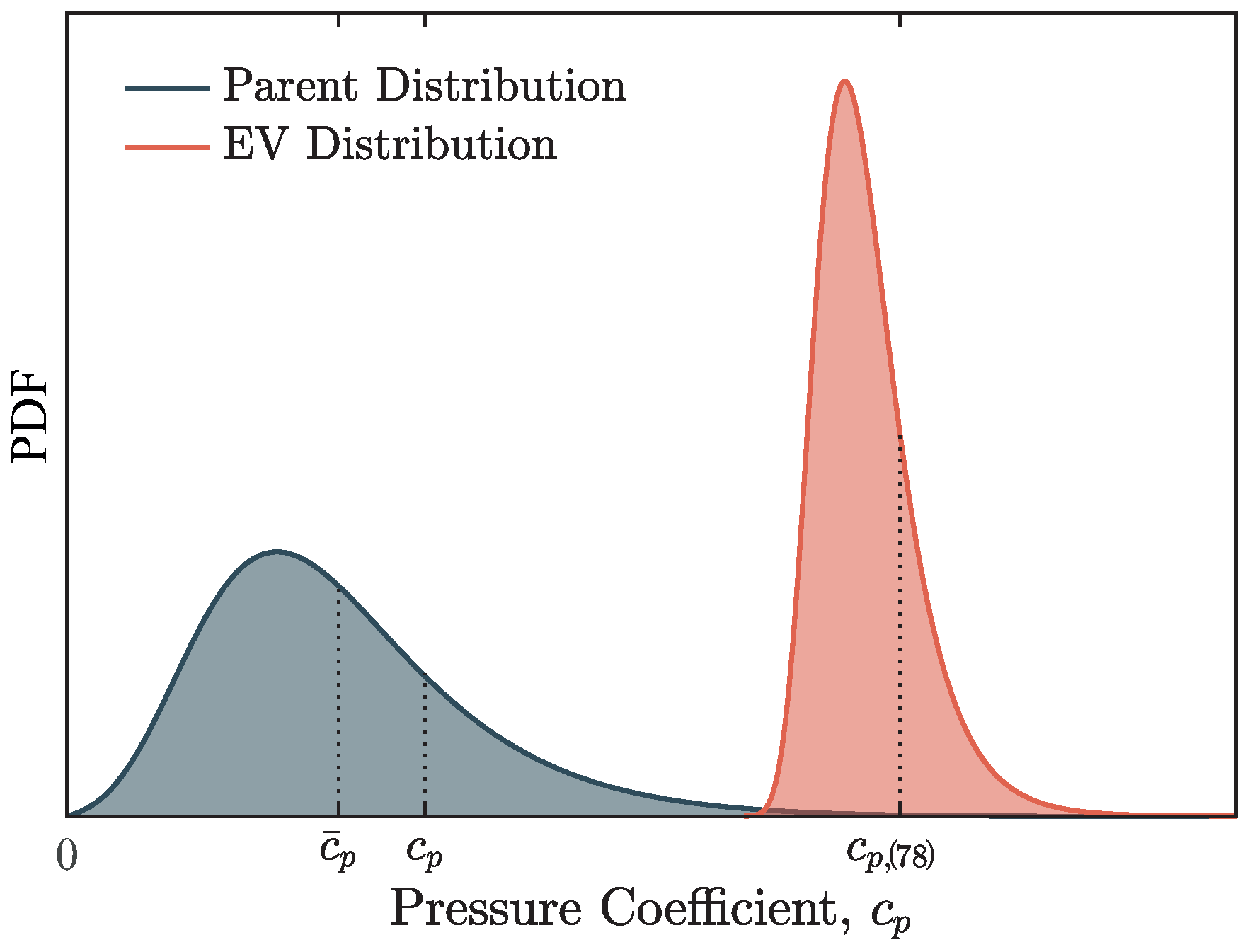
It was then clear that turbulent fluctuations do not immediately translate into pressure fluctuations, at least at points where the flow is separated, and this suggested a revision of the quasi steady approach. Based on the observation that it is impossible to separate the components of the pressure fluctuation deriving from the oncoming turbulence from those deriving from signature turbulence, an alternative to the Davenport’s approach is that of combining the mean velocity pressure with a tail statistics of the pressure coefficient. A first attempt in this direction was that of [23], who proposed to determine the design value of pressure coefficients as those corresponding to the $5\times {10}^{-4}$ fractile of the parent distribution. The chosen probability level corresponds to the largest gust in one hour having a duration of $1.8\mathrm{s}$, as suggested by Eaton and Mayne [24].

Once it is recognized that the pressure coefficient is to be calibrated as a value corresponding a low probability of exceedance, then the question arises of whether it is more appropriate to consider the parent population or to apply Extreme Value (EV) analysis. For the latter option, it is observed that the domain of attraction of parents with an exponential tail is the Type I EV distribution or Gumbel distribution [25].

In their pioneering work, Cook and Mayne [26] tried to find a statistical model from which to derive the pressure coefficients, as alternative to the use nominal values (corresponding to mean values) as reported in the UK Code of Practice for wind load [27]. They proposed a design approach in which the definition of both wind speed (or velocity pressure) and pressure coefficients is based on the Spectral Gap [17]:

• The design value of wind speed is obtained as an EV statistics of the wind speed, U, averaged over a period T of $10\min$ or $1\mathrm{h}$, including all fluctuations of the macro-meteorological peak;
• The design value of the pressure coefficient, $c_p$, is the peak value within the averaging period T, including all the micro-meteorological fluctuations of the incident wind turbulence, as well as those coming from signature turbulence.

As already pointed out by Davenport [14], in this case the peak pressure coefficient is also not to be confused with a maximum instantaneous value measured at a point, but it is rather a statistics the time- and space-averaged instantaneous values:

$$c_{p,\tau ,A}\left(t\right)=\frac{1}{A}{\displaystyle \frac{1}{\tau }}{\int }_A{\int }_{t-\tau /2}^{t+\tau /2}{c}_p(a,\overline{t})\mathrm{d}\overline{t}\mathrm{d}a$$

(12)

The duration $\tau$ and the averaging area A shall be related to the capacity that the load has to produce an effect; for example, the load duration needed to produce damage to cladding elements is smaller than that needed to produce damage on structural elements having larger tributary areas. The averaging duration and averaging area can be related with each other, once the convective nature of the process is recognised. A common relationship between the characteristic dimension $l=\sqrt{A}$ of the averaging area and the averaging duration is provided by the TVL formula [28]:

$$\tau U=4.5l$$

(13)

The choice either A or $\tau$ allows the use of Equations (12) and (13). Common practice is to select A as the tributary area of the structural member or cladding element under consideration.

Therefore, in the approach of Cook and Mayne both mean wind speed and pressure coefficients have to be understood as statistical variables and their design values need to be assessed by EV analysis. The mean wind speed is usually evaluated with a yearly probability of exceedance equal to $0.02$, corresponding to a return period $R=50\mathrm{yrs}$; the same yearly probability of exceedance applies also to wind loads. Therefore the statistics of the pressure coefficient has to be chosen such that combined with a velocity pressure having a yearly probability of exceedance of $0.02$ provides a wind load having also a yearly probability of exceedance of $0.02$. Assuming a Type I EV distribution for both the annual maximum wind speed and the coefficient of pressure, Cook and Mayne [26] recommended the use of the $78\%$ fractile of peak pressure coefficients. The Cook–Mayne coefficient was established for the UK wind climate and is used worldwide. Indeed, if a more reliable value is to be obtained, then it should be calibrated on the specific climate of the site of interest.

5. Calibration of Pressure Coefficients

5.1. Codification Procedures

EV analysis for the evaluation of the design pressure coefficients has been accepted worldwide. An exhaustive literature review of the evolution and of the geographic differences in the evaluation of pressure coefficients was presented by Gavanski et al. [29], while a state-of-the-art of the methods to estimate the peak pressures was made by Gavanski and Cook [30]. In Europe, the method of Cook and Mayne is widely used for the evaluation of the maximum and minimum pressure coefficients. Despite this, the sources of building pressure coefficients include both, largest measured peaks [31] and $78\%$ fractiles [32] resulting from EV analysis [33,34]. In fact, the current version of Eurocode 1 [35], proposes two sets of pressure coefficients for the assessment of (1) local pressures on cladding and roofing elements ($c_{pe,1}$, for loaded areas of $1{\mathrm{m}}^2$ corresponding to the largest measured peaks) and (2) wind loading on resistant structural members ($c_{pe,10}$, for loaded areas of $10{\mathrm{m}}^2$, corresponding to $78\%$ fractiles).

Current Codes and Standards incorporate the gust factor approach by using an equivalent form of Equation (7), expressing the characteristic wind load at a point M as:

$$w\left(M\right)=q_{m,ref}·G_{w,lin}·c_p\left(M\right)$$

(14)

where $q_{m,ref}=0.5·\rho ·v_m^2\left(z_{ref}\right)$ and $v_m\left(z_{ref}\right)$ are the mean velocity pressure and mean wind speed at height $z_{ref}$ above the ground, corresponding to a yearly probability of exceedance of $0.02$, or a return period $R=50\mathrm{yrs}$, respectively, and $c_p\left(M\right)$ is the representative value of the pressure coefficient at the point:

$$c_p\left(M\right)={\displaystyle \frac{\widehat{p}\left(M\right)}{\widehat{q}\left(z_{ref}\right)}}$$

(15)

where $\widehat{p}\left(M\right)$ is the peak relative surface pressure measured in the wind tunnel at point M, and $\widehat{q}\left(z_{ref}\right)$ is the peak velocity pressure measured in the wind tunnel at height $z_{ref}$ above the tunnel floor. Therefore, the height $z_{ref}$ to be used in Equation (14) should be the same as that used for the normalization of the pressure coefficient in Equation (15).

Unlike the gust factor approach of Davenport, the method of Cook and Mayne accounts for wind gustiness through the pressure coefficients. These incorporate the effects of both the oncoming and signature turbulence, and may strongly deviate from a Gaussian behaviour. Instead of Equation (14), the wind loading turns out to be:

$$w\left(M\right)=q_{m,ref}·c_{p,\left(78\right)}\left(M\right)$$

(16)

where $c_{p,\left(78\right)}\left(M\right)$ indicates the 78% fractile of the pressure coefficient at point M.

Comparing Equations (14) and (16) one obtains:

$$c_p\left(M\right)={\displaystyle \frac{c_{p,\left(78\right)}}{G_{w,lin}}}$$

(17)

The normalization procedure in Equation (17) gives rise to the so-called pseudo-steady pressure coefficient, highlighting the fact that it is calibrated within the steady-state method.

Figure 2 sketches the parent and the EV distributions of the pressure coefficient. The figure should help understanding the probabilistic nature of the pressure coefficients and the differences between mean (${\overline{c}}_p$), $78\%$-fractile ($c_{p,\left(78\right)}$) and pseudo-steady ($c_p$) pressure coefficients.

5.2. Pressure Coefficients Analysis

Codes and Standards provide pressure coefficients $c_p$ for rectangular buildings with flat roofs with different corner arrangement (sharp, curved, mansard, and with parapets) as well as with pitched roofs. When the geometry of interest is not covered by the Code or Standard, it is necessary to resort to wind tunnel tests to quantify the pressure coefficients.

The result of a wind tunnel test is a dataset consisting of time histories $c_p(M;t)$ of the pressure coefficients at a number of measurement points M on the model building surfaces. The instantaneous pressure coefficient is calculated as:

$$c_p(M;t)={\displaystyle \frac{p(M;t)-p_{\mathrm{o}}}{q_{m,ref}}}$$

(18)

in which $p(M;t)$ is the absolute surface pressure measured at point M and time t, and $p_{\mathrm{o}}$ is the static air pressure in the region outside the influence of the body (barometric pressure). In most cases, the reference height $z_{ref}$ for pressures is taken equal to the building height h, therefore $q_{m,ref}=q_{m,h}$. In some cases, the pressure coefficients are normalized with respect to a reference wind tunnel height $z_{wt}$. In the latter case, preliminary to the statistical treatment of the data, the measurements must be converted to the reference height $z_{ref}$:

$$c_p(M;t)={\displaystyle \frac{q_{m,wt}}{q_{m,ref}}}·c_{p,wt}(M;t)$$

(19)

in which $c_{p,wt}(M;t)$ is the pressure coefficient normalized with respect to the velocity pressure $q_{m,wt}$ at the height $z_{wt}$.

The datasets provided by wind tunnel tests are sampled at frequency $f_s$, corresponding to a sampling time $1/f_s$ usually smaller than the averaging period $\tau$. Therefore the time histories of the measured pressure coefficients must first be converted into time histories of $\tau$-averaged pressure coefficients, also corresponding to area-average as per the TVL formula. Thus, a moving-average is applied to the time series:

$$c_{p,A}(M;t)={\displaystyle \frac{1}{\tau }}{\int }_{t-\tau /2}^{t+\tau /2}{c}_p(M;\overline{t})\mathrm{d}\overline{t}$$

(20)

corresponding to low-pass filtering the measured time series at a frequency $1/\tau$. For example, Cook [32] referred to a load duration $\tau =1\mathrm{s}$ and to a common design wind speed for the UK $U=22.5\mathrm{m}/\mathrm{s}$, which correspond to an averaging area $A=12.5{\mathrm{m}}^2$ (or a characteristic dimension $l=5\mathrm{m}$, corresponding to the diagonal of a square area). By doing this, the values given in Eurocode 1 as $c_{pe,10}$ are obtained (where the subscript e stands for external, as opposed to i used for internal pressures). On the other hand, when wind tunnel time series of the point pressure coefficients are available, Equation (20) must be evaluated with:

$$\tau =4.5{\displaystyle \frac{\sqrt{A}}{v_{m,ref}}}$$

(21)

where A is the tributary area of the loaded structural element, and $v_{m,ref}$ is the expected value for the design mean wind speed.

The concept of tributary area applies to secondary structural elements or cladding elements; therefore, it is in the order of few square meters. For main structural elements and for foundation loads, where the tributary area is much larger, besides the use of Equation (20), the reduction in the resulting loads arising from the lack of coherence of the oncoming flow is accounted for through a background factor. This issue was first addressed by Davenport [13], who introduced the notion of background factor $B^2$, taking into account not only the lack of correlation of the oncoming flow turbulence, but also the vertical variation of the mean wind speed. In particular, the background factor is expressed as a function of the ratio $\sqrt{A_l}/L_u$ between the characteristic dimension of the loaded area $A_l$ and the turbulent length scale $L_u$. In so doing, within the gust factor approach, the equivalent (or peak) load $W_{lin}$ is given by:

$$W_{lin}=0.5\rho U^2·c_p·G_{W,lin}\left(A_l\right)·A_l$$

(22)

where:

$$G_{W,lin}\left(A_l\right)=1+2g_{W,lin}{I}_u\sqrt{B^2\left(A_l\right)}$$

(23)

is the gust loading factor depending on the loaded area, and $g_{W,lin}$ is the associated peak factor. It is clear that when the characteristic dimension of the structure is small compared with the dimension of the turbulent eddies, then $B^2\to 1$. Similar to $g_{w,lin}$, a value of $3.5$ is adopted by Eurocode 1 also for $g_{W,lin}$. A recent summary can by found in Liu et al. [36].

For the equivalent load, only a linearized version is given; this derives from the fact that the background factor in Equation (23) is derived following a stochastic approach in the frequency domain, in fact needing a linear relationship between the wind velocity fluctuations and the surface pressure fluctuations.

Finally, once the time series of pressure coefficients are normalized with respect the reference height $z_{ref}$, and filtered according to the load duration $\tau$, then EV analysis can be performed. When a Type I EV distribution is used for the extremes of the pressure coefficient, then the Gumbel scale ${\mu }_M$ and shape ${\beta }_M$ parameters are evaluated at each measurement point M. Then, the $78\%$ fractile of the pressure coefficient is evaluated as:

$$c_{p,\left(78\right)}\left(M\right)={\mu }_M+1.4·{\beta }_M$$

(24)

5.3. Example

The above procedure is applied to pressure measurements on the flat roof of a building with dimensions $b=24.40\mathrm{m}$, $d=38.10\mathrm{m}$, $h=12.20\mathrm{m}$, to evaluate the pressure coefficients $c_{p,1}$ for roof cladding and $c_{p,10}$ for structural elements. The raw data are taken from the NIST database [37]. First, a moving-average is applied to the original time series by considering a mean wind speed of $26.5\mathrm{m}/\mathrm{s}$, giving $\tau =0.25\mathrm{s}$ for $c_{p,1}$ and $\tau =0.76\mathrm{s}$ for $c_{p,10}$. Then, the Gumbel parameters ${\mu }_M$ and ${\beta }_M$ in Equation (24) are calibrated based on the filtered time series, and the values of $c_{p,\left(78\right)}$ are calculated.

Figure 3a–d and Figure 4a–d show the contour plots of pressure coefficients $c_{p,1}$ and $c_{p,10}$, respectively, evaluated as in Equation (17), for wind angles of incidence of $0^{\circ }$, ${15}^{\circ }$, ${30}^{\circ }$, and ${45}^{\circ }$. Figure 3e and Figure 4e show the envelope of the calculated values, together with the zoning proposed by Eurocode 1.

With the purpose of assessing roofing elements, the envelope of Figure 3e can be used, as what we are interested in is the maximum wind load obtained from an omnidirectional analysis. For secondary structural members with small to moderate tributary areas, up to about $10{\mathrm{m}}^2$, the $c_{p,10}$ envelope of Figure 4e can still be used. However, in the case of larger tributary areas, i.e., for main structural elements or for foundation loads, the background factor needs to be considered. In this case, the pressure coefficients $c_{p,10}$ provided by the loading patterns of Figure 4a–d shall be used for directional analysis, in conjunction with a background factor $B(A_l=b·d)$.

In

Table 1. Comparison of area-averaged coefficients from the analysis of NIST data (Current Work, CW) and Eurocode 1 values (EC1).

Roof Zone	${\mathit{c}}_{\mathit{p},1}$		${\mathit{c}}_{\mathit{p},10}$
	CW	EC1	CW	EC1
F	$-2.18$	$-2.5$	$-1.96$	$-1.8$
G	$-1.52$	$-2.0$	$-1.25$	$-1.2$
H	$-1.11$	$-1.2$	$-0.91$	$-0.7$
I	$-0.53$	$-0.2$	$-0.37$	$-0.2$

, a comparison of the area-averaged coefficients from the analysis of NIST data (CW) and Eurocode 1 values (EC1) is presented. The discrepancy between the corresponding values can be partly ascribed to the fact that the values given in Eurocode 1 apply to different ratios b:d:h; therefore, they must in some way smooth out the differences between one case and another.

6. Future Developments

According to the procedures developed through the years, the assessment of the wind load on rigid buildings requires the knowledge of both return velocity pressure and statistics of pressure coefficients. As already pointed out, pressure coefficients available in current Codes and Standards suffer from a number of deficiencies:

• They refer to a rather narrow variety of geometries, often limited to rectangular plan buildings with constant height; for geometries that can be schematized as an assemblage of rectangular elements, empirical criteria are given to extend the use of pressure coefficients measured for rectangular buildings;
• The statistical definition of the available pressure coefficients is not always clear, and seldom complies with Equation (24);
• The duration of the load $\tau$ used in Equation (12), usually between $1\mathrm{s}$ and $3\mathrm{s}$, had in some cases proven inadequate when assessing cladding loads in areas of strong negative pressures, a smaller value being more appropriate. This is the effect of high suctions being strongly non-Gaussian; therefore, featuring high peak factors;
• The use of envelopes of pressure coefficients averaged over small areas for the assessment of main structural members and foundation load proves inaccurate; as an alternative, a more refined directional analysis using influence coefficients would be appropriate.

On the other hand, velocity pressures also suffer from a number of limitations:

• Extreme wind maps are often old, and produced with heterogeneous data and heterogeneous (and often out-of-date) statistical methods;
• There is often non appropriate consideration of the various storm mechanisms;
• Very seldom the measurements are continuous, therefore giving rise to an underestimation of the design wind speed as an effect of downsampling.

In recent years, the development of Web and Information Technologies has led to new opportunities for more reliable procedures in the assessment of structural safety. At the beginning of the 21st century, the University of Notre Dame founded the NatHaz (Natural Hazards) Modeling Laboratory with the aim ”to quantify load effects caused by various natural hazards on structures and to develop innovative strategies to mitigate and manage their effects” [38]. The NatHaz website was published, providing a collection of aerodynamic and damping datasets, online design modules for low- and high-rise buildings, and other features for buildings design to wind load. At the same time, the National Institute of Standards and Technology (NIST) developed a Database-Assisted Design (DAD) software for low- and high-rise buildings, freely available on the NIST website [39]. The software of both Institutions are based on the availability of aerodynamic databases. In this framework, NIST and the Tokyo Polytechnic University (TPU) provided data collections to create databases of pressure coefficients (aerodynamic database) and mechanical properties of buildings.

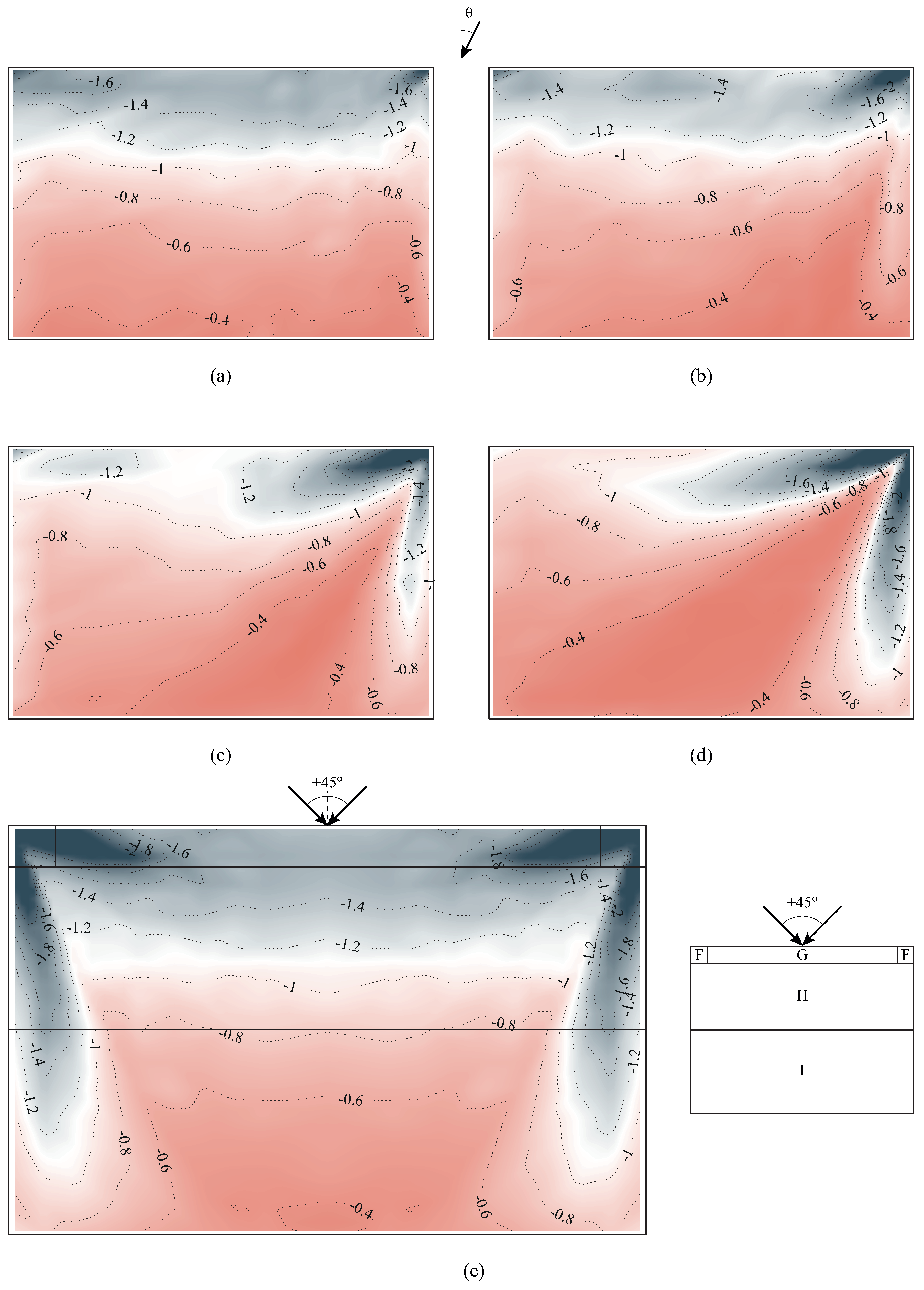
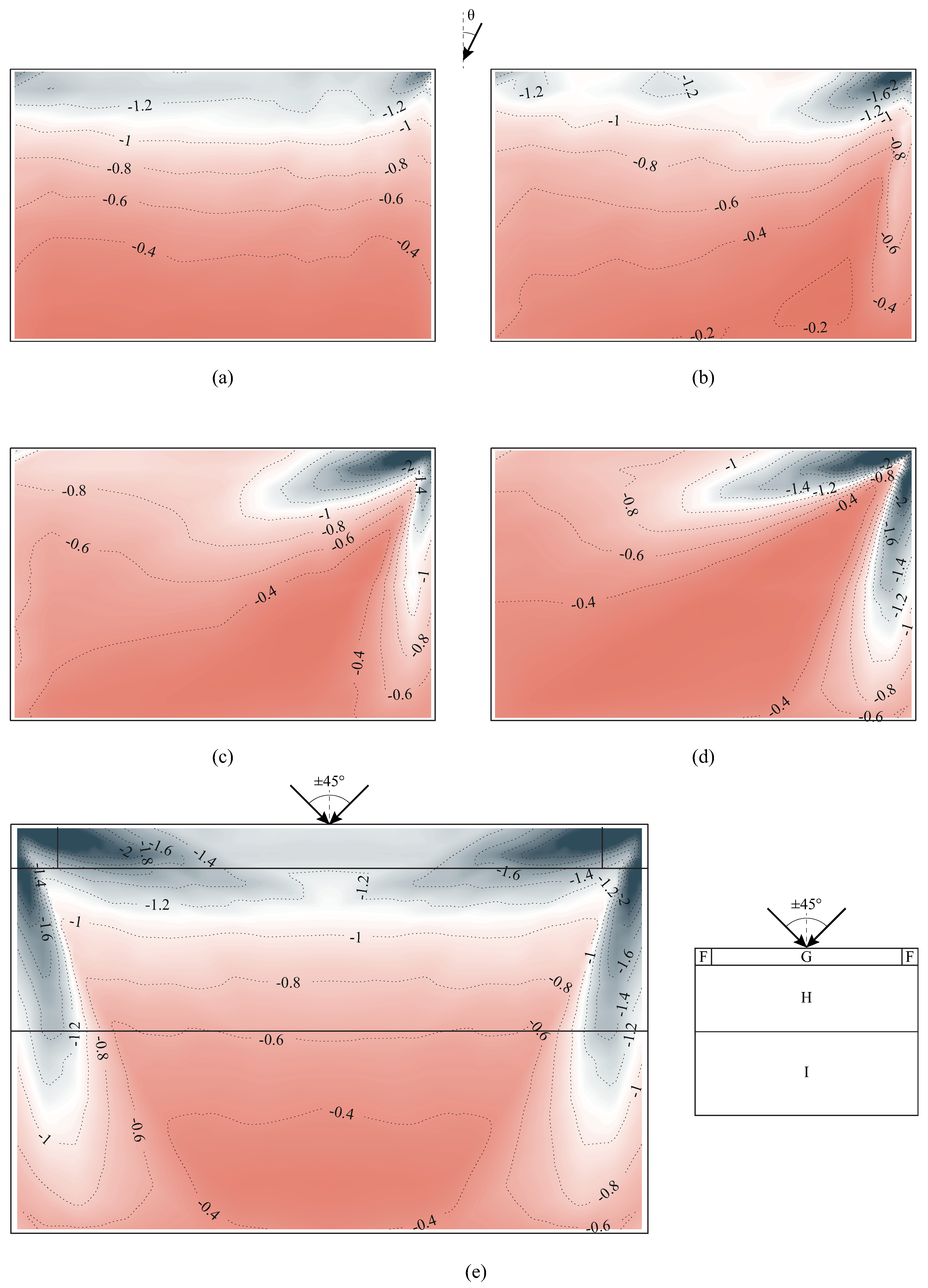
The NIST database collects data measured at the Boundary Layer Wind Tunnel Laboratory (BLWTL) of the University of Western Ontario (UWO); it is the result of a joint study conducted by NIST and Texas Tech University (TTU) entitled ’Windstorm Mitigation Initiative: Wind Tunnel Experiments on Generic Low Buildings’ [37]. Instead, the TPU database is part of the 21st Century Center of Excellence Program named ’Wind Effects on Buildings and Urban Environment’ [40]. The characteristics of the wind tunnel tests are summarized in

Table 2. Main aerodynamic databases for isolated low-rise buildings.

	Unit	NIST [37]	TPU [40]
Sampling Frequency *, $f_s$	$\mathrm{Hz}$	500	500
Sampling Period *, $T_s$	$\mathrm{s}$	100	18
$10\mathrm{cm}$ Wind Speed *, $v_{m,10}$	$\mathrm{m}/\mathrm{s}$	$8.8$	$7.4$
Length Scale, ${\lambda }_l$		1:100	1:100
Velocity Scale, ${\lambda }_v$		1:4	1:3
Roughness Category		Open Country, Suburban	Suburban
Width × Depth, $b\times d$	$\mathrm{m}$	$12.2\times 19.0$, $24.4\times 38.1$, $15.2\times 30.5$, $15.2\times 53.3$, $36.6\times 57.1$, $48.8\times 76.2$	$16.0\times 16.0$, $16.0\times 24.0$, $16.0\times 40.0$
Height, h	$\mathrm{m}$	$3.7$, $4.9$, $5.5$, $7.3$, $9.7$, $12.2$	$4.0$, $8.0$, $12.0$, $16.0$
Roof Slope, $\alpha$	${}^{\circ }$	$1.2$, $2.4$, $4.8$, 14, 27	0, $4.8$, $9.4$, 14, $18.4$, $21.8$, $26.7$, 30, 45

for both aerodynamic databases. As discussed in Section 5.2, the data provided in the databases can be used to calculate point surface pressure coefficients and area-averaged surface pressure coefficients on roof and wall surfaces, as well as foundation loads on low-rise buildings. Aerodynamic databases can be expanded in the future, to incorporate data for less regular geometries; these can come either from systematic studies on a variety of geometries (e.g., [41]), or from specific project-related analyses (e.g., [42]).

Currently wind tunnel tests are considered the reliable tool for investigating building aerodynamics, the main concern with Computational Fluid Dynamics (CFD) being the difficulty in calibrating simulations and validating their results. However, with the purpose of building aerodynamic databases, a joint effort within the scientific community might be able to produce standard criteria for simulations, the results of which may in a future complement wind tunnel data.

On the other hand, research is currently being developed towards the possibility of using reanalysis data for the definition of extreme wind climate at sites of interest. Numerical Weather Prediction (NWP) models simulate the physics of the atmosphere using available observations, and calculate meteorological variables in a three-dimensional grid extending from the surface to the stratosphere. These models have traditionally been used for weather forecasting, but they may also be rerun to produce a set of historical data. For example, the Integrated Forecast System (IFS) at the European Centre for Medium-Range Weather Forecasts has been rerun to produce a global reanalysis from 1979 to present at a horizontal resolution of 31 km, known as the ERA5 reanalysis [43]. The resolution of ERA5 is too coarse for calculating extreme values at a specific site, and downscaling to a higher resolution is hence required. This can be accomplished by rerunning the NWP model at higher resolution within the ERA5 dataset, which is called dynamical downscaling. An example, the NORA10 dataset [44] was created by running a NWP model with 11 km resolution, covering most of Northern Europe. The dataset is currently being updated with new model runs at 3 km resolution. Dynamical downscaling has the advantage that the physical consistency between the different variables is retained, but it is computationally demanding therefore it is not suitable to produce a long dataset. A cheaper alternative is running a high-resolution model for a shorter period, and use the short dataset for finding a statistical relationship between the short high-resolution dataset and the long low-resolution dataset. This method is called statistical downscaling [45].

The quality of these modelled dataset depends on the NWP model used and on its resolution, as well as on the methods used in statistical downscaling and interpolation; validation of the data against observation is clearly necessary for these datasets to become of practical use. In particular, it is observed that some models tend to underestimate the strongest winds. Not all NWP datasets include wind speed and direction as an explicit output. Examples of datasets of possible use when assessing wind loads are: the SMHI HARMONIE-ALADIN, covering the entire of Europe for the period 1961 to 2016 at a horizontal resolution of 11 km [46]; the MESCAN-SURFEX analysis, covering the period from 1961 to 2015 at 5 km spatial resolution [47]; the NORA10/NORA3 datasets, covering the period 1957 to 2002 for Scandinavia, Britain and parts of Northern Europe at 11 km resolution and the period 1995 to 2020 at a 3 km resolution [44]; and the Klinogrid dataset, providing hourly wind speed and wind direction on a 1 km resolution grid for the period 1957 to 2015 [45].

The visionary Wind Engineer can therefore think of a future in which web-based apps will access online databases to retrieve aerodynamic and meteorological data, and combine them together to obtain the “best” estimate of the wind load on a project structure; and machine learning and big data analytics could be the tools to achieve that. How far that future can be, and whether we will ever see it we do not know.