
Multifactorial Chloride Ingress Model for Reinforced Concrete Structures Subjected to Unsaturated Conditions


Abstract
:1. Introduction
1.1. Background
1.2. Problem Statement
- 1.
- a multifactorial diffusion model for the diffusion zone detailed in Section 2;
- 2.
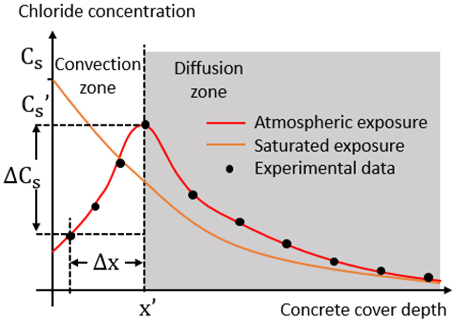
- a procedure and models for lifetime assessment that provide an equivalent surface chloride concentration (Cs′) in the boundary between the convection and diffusion zones that is located at the distance x′ from the concrete surface (see Figure 1). These procedures and models are described in Section 3 and illustrated in Section 4.
2. Multifactorial Chloride Ingress Model for Pure Diffusion Zones
2.1. Model Formulation
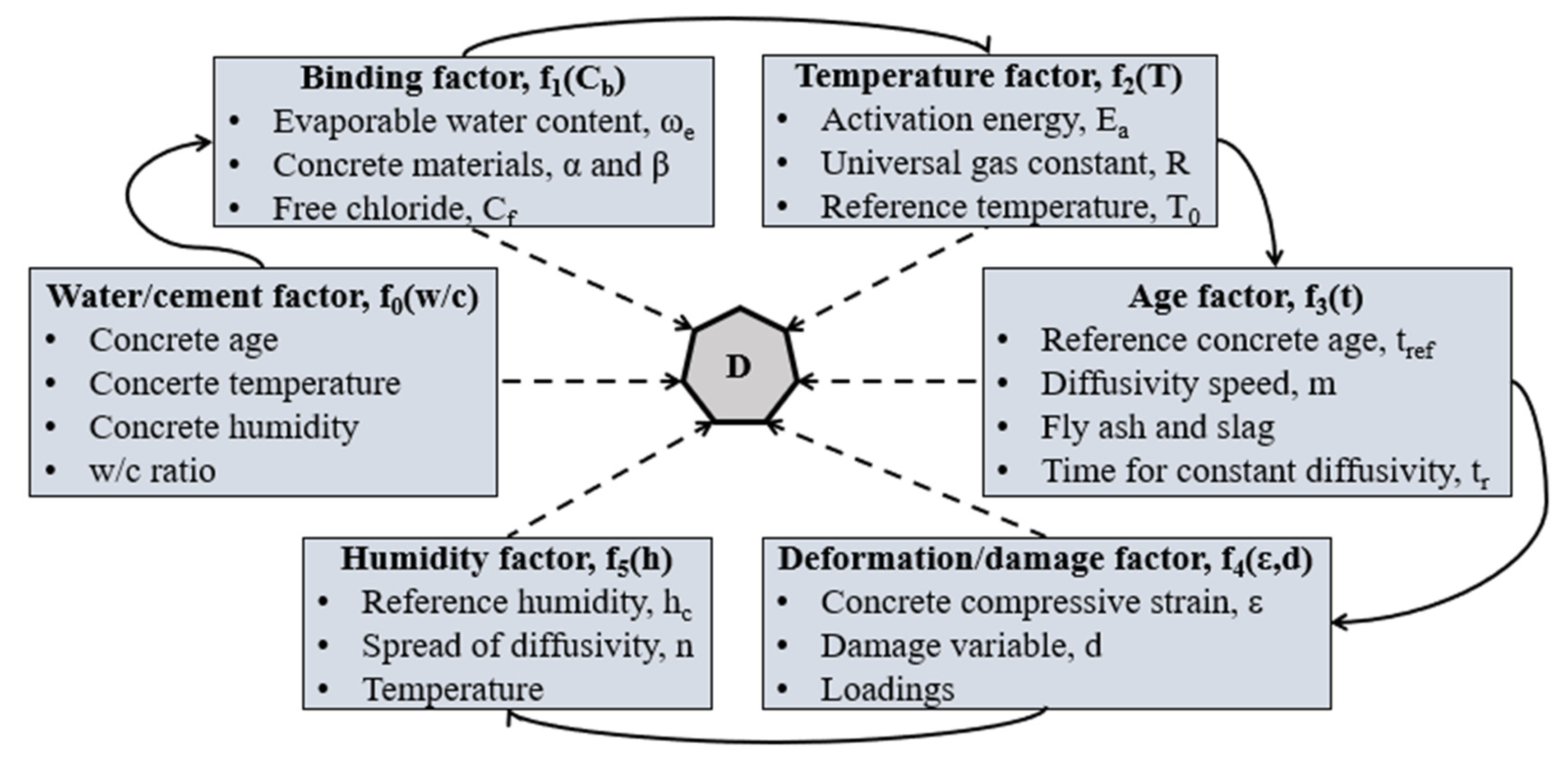
- f0: age, temperature, humidity of concrete; w/c ratio [42].
- f1: ωe, α, β, Cf (Equation (6)).
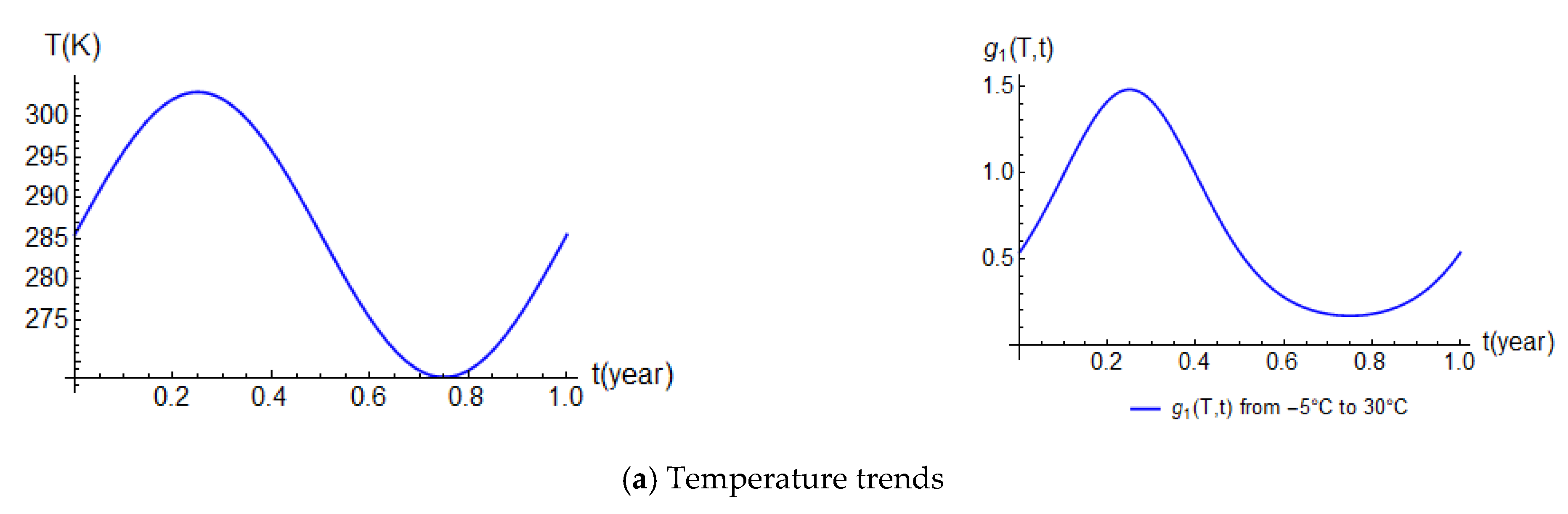
- f2: Ea is the activation energy of the diffusion process that depends on the type of cement and w/c ratio; R is the universal gas constant that depends on the chemical potential of ions, molar concentration, and temperature [31]; T0 is the reference temperature [45] (see Section 3.1).
- f3: tref, tr, m (Equation (5)).
- f4: d, ε and its corresponding load [16]. This factor can be called as “loading factor” and depends on several conditions as the properties of concrete, such as the sinuosity and the shrinkage degree of capillary pores. For this, it is complicated to be estimated as shown in [38,42]. In this paper, it is considered as a constant value.
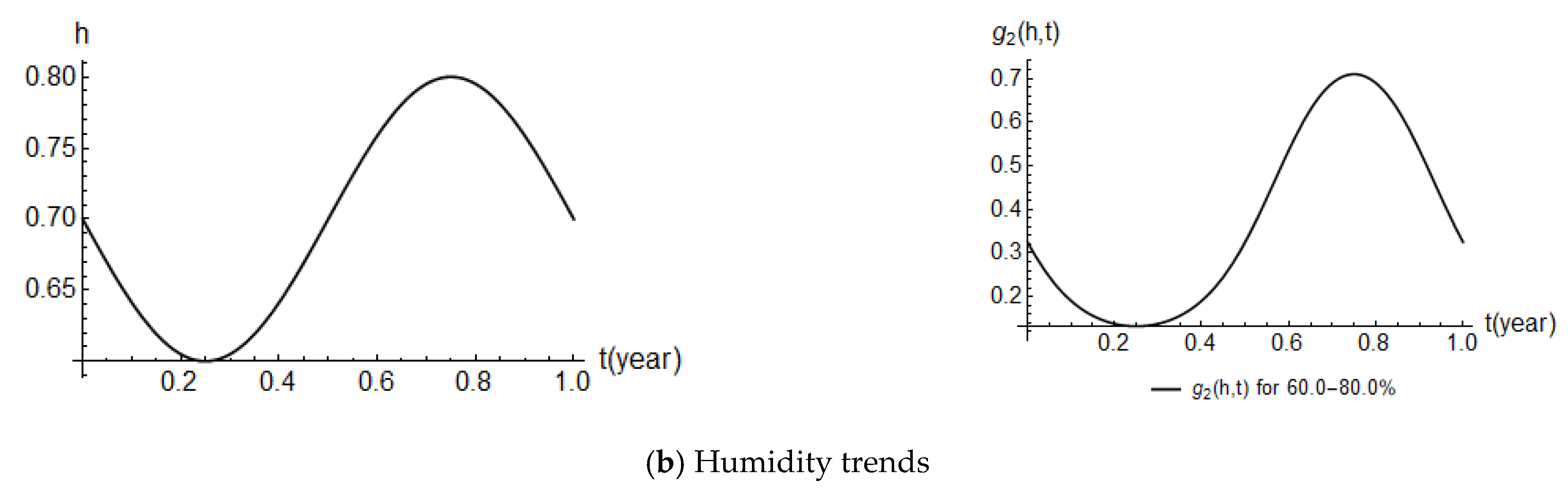
- f5: hc is the humidity, at a certain temperature, at which D drops halfway between its maximum and minimum values; n is a value that characterizes the spread of the drop in D [46] (see Section 3.1).
2.2. Numerical Solutions
2.2.1. Constant Diffusivity
2.2.2. Non-Constant Diffusivity
3. Proposed Chloride Ingress Model for Unsaturated Conditions
- Concrete is homogenous and subjected to an atmospheric chloride condition at x ≥ 0.
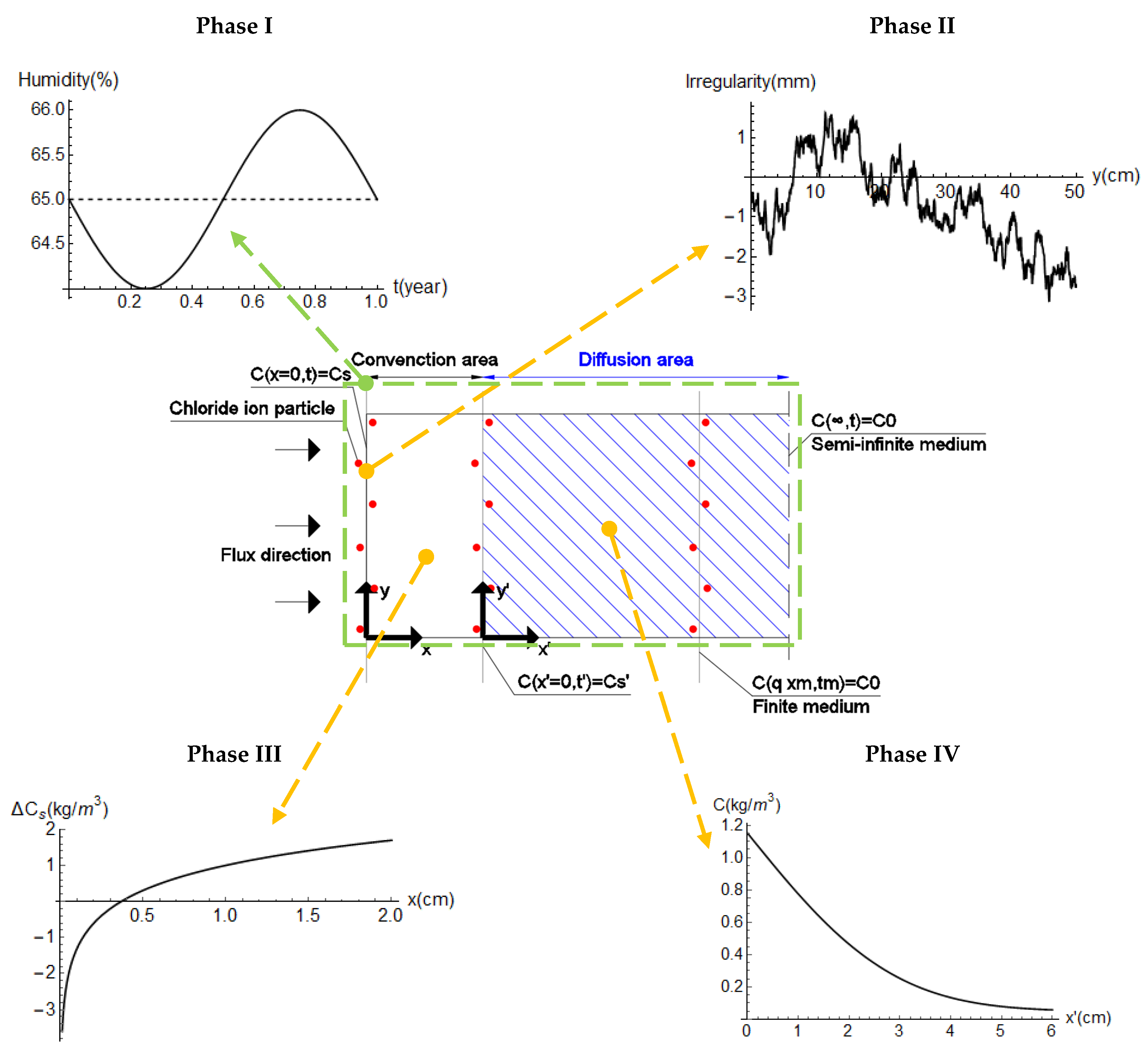
- Two different axis systems are defined: x, y, and x′, y′ to differentiate between the convection and diffusion areas (Figure 3).
- Fick’s laws (pure diffusion) are only valid for x′ ≥ 0 (diffusion area).
- The diffusion process is unidimensional and is purely mechanical.
- The concrete element is a finite medium described by Equation (15).
- The convection process depends on x-axis.
- D is considered non-constant and multi-factorial.
- The external environment conditions (humidity and temperature) are periodic for a year and vary in t.
- The effects of concrete surface irregularities on Cs are considered.
- There is a difference of Cs, i.e., ΔCs = Cs′ − Cs, from x = 0 to x′ = 0.
- An inner chloride concentration C0 is considered constant and is added to Cs.
3.1. Phase I: External Environmental Conditions
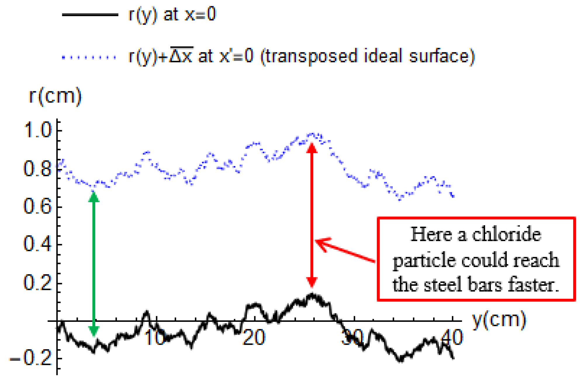
3.2. Phase II: Surface Concrete Irregularities
3.3. Phase III: Changes on Cs Due to Unsaturated Conditions
- For laboratory tests: 1 month of exposure time under the mean values of T = 20 °C and h = 60.0% [29]; 14 days of exposure time under dry/wet cycles (extreme level of aggressiveness) [28]; 8 weeks of exposure time [30]; 60 months of exposure time in the tidal zone (extreme level of aggressiveness) [13].
3.4. Phase IV: Chloride Ion Diffusion
4. Numerical Examples
4.1. Problem Description and Used Materials
4.2. Description of Analysed Cases
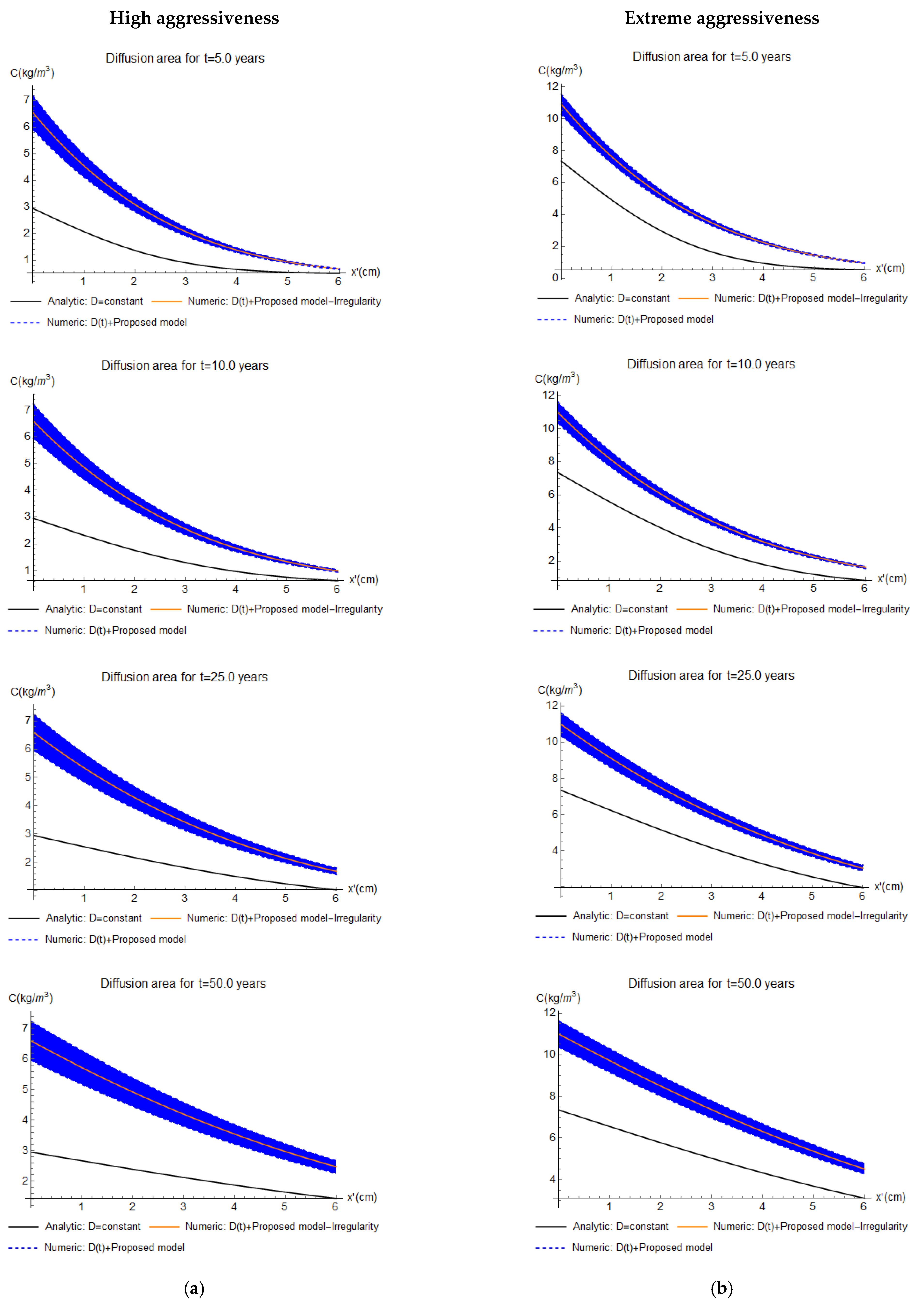
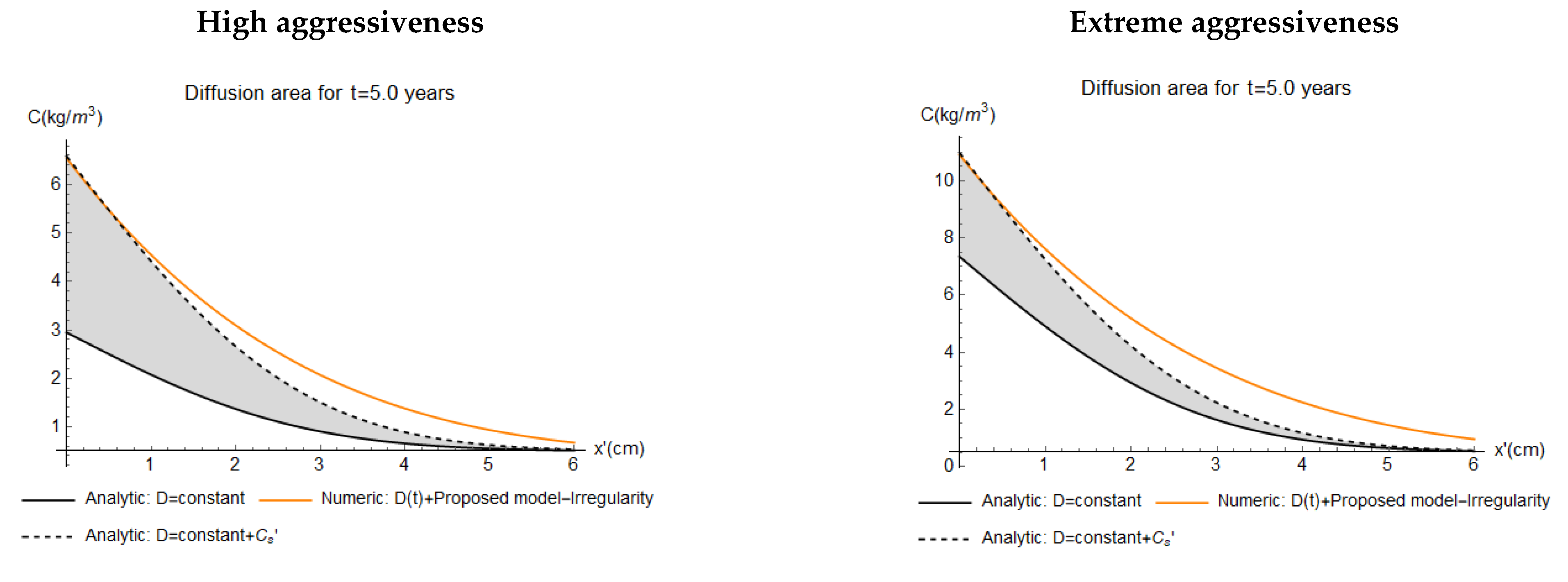
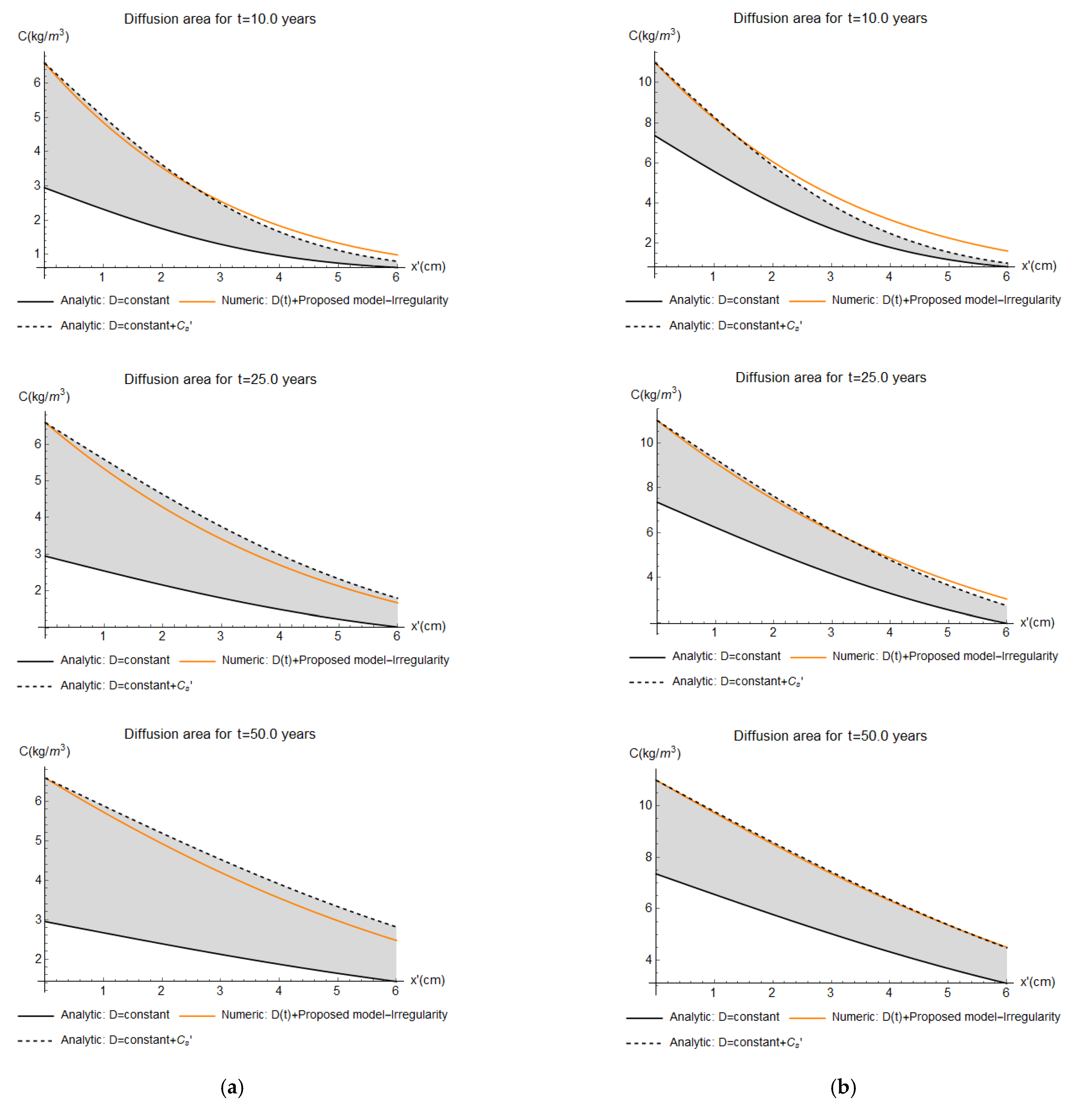
- Dashed black line: analytical results like the previous case plus the contribution of Cs′. In this case, it is possible to see the impact of the convection area where Cs increases (grey area) and the effects of the non-constant D.
- Dashed blue line: numerical results by Equation (11) considering the non-constant multifactorial D and the proposed model shown in Figure 3. Due to the amplitude of the irregularity profile, an upper curve and a lower curve are plotted, which represent the chloride contents for the r(y)max and r(y)min, respectively. Therefore, the effects of the irregularity are represented by the filled blue area. For each analysis, a different irregularity profile is generated, but its random variability is imperceptible since maintains substantially constant.
- 4.
- Solid orange line: numerical results like analysis 3 but without the irregularity effects (i.e., r(y) = 0).
4.3. Results
5. Conclusions
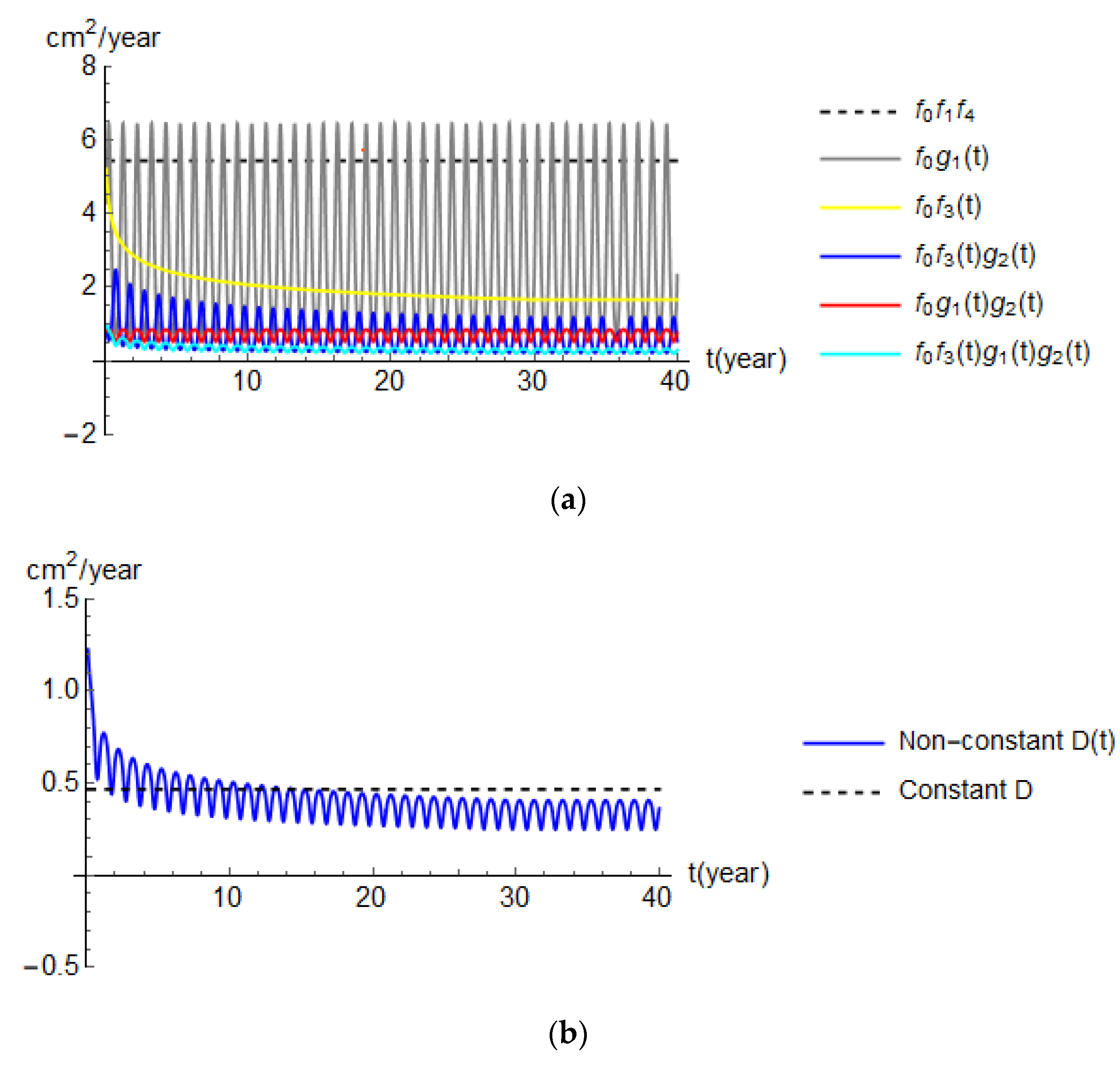
- The diffusivity D, which is the key parameter of the mechanical diffusion process, should account for the w/c ratio, chloride binding, variations of temperature and humidity, concrete aging, concrete deformation, and damage. This paper used a new complete multi-factorial D (Equation (4)) that includes 20 sub-factors to estimate in a more realistic way the chloride ingress process. It is shown that up to ~10 years the non-constant D is higher than the constant D, and therefore, the chloride concentration in RC structures by using a constant D could be underestimated. After ~15 years the situation is the opposite; however, an underestimation of the chloride attack for the early service life could increase corrosion initiation risks.
- From literature, 136 values have been collected to find two parameters characterizing the convection zone ( and ). Both parameters were integrated into the proposed multi-phase model (see Figure 3) to estimate the evolution of chloride concentration inside non-saturated concrete. From the results of the numerical example, it is possible to affirm that the consideration of convection effects is crucial to improve the accuracy of the prediction models. Further research will focus on the experimental validation of the proposed approach.
- Numerical solutions by using HPs have been carried out to develop the proposed model in a dynamic way. Due to the variability of some factors and parameters, only by advanced numerical solutions, it could be possible to plot good approximations of chloride concentrations in concrete. The results show that the analytical solutions could underestimate the chloride concentration C for period t < 10 years and for x′ > 4.0 cm.
Author Contributions
Funding
Institutional Review Board Statement
Informed Consent Statement
Data Availability Statement
Acknowledgments
Conflicts of Interest
References
- Meira, G.R.; Andrade, M.C.; Padaratz, I.J.; Alonso, M.C.; Borba, J.C., Jr. Measurements and modelling of marine salt transportation and deposition in a tropical region in Brazil. Atmos. Environ. 2006, 40, 5596–5607. [Google Scholar]
- Valdes, C.; Castañeda, A.; Corvo, F.; Marrero, R.; Montero, R. Atmospheric corrosion study of carbon steel in Havana waterfront zone. In Proceedings of the International Conference of Sustainable Production and Use of Cement and Concrete, Villa Clara, Cuba, 23–30 June 2019; Martirena-Hernandez, J., Alujas-Díaz, A., Amador-Hernandez, M., Eds.; RILEM Bookseries; Springer: Cham, Switzerland, 2020. [Google Scholar]
- Guerra, J.C.; Castañeda, A.; Corvo, F.; Howland, J.J.; Rodriguez, J. Atmospheric corrosion of low carbon steel in a coastal zone of Ecuador: Anomalous behaviour of chloride deposition versus distance from the sea. Mater. Corros. 2019, 70, 444–460. [Google Scholar] [CrossRef]
- Ou, Y.C.; Fan, H.D.; Nguyen, N.D. Long-term seismic performance of reinforced concrete bridges under steel reinforcement corrosion due to chloride attack. Earthq. Eng. Struct. Dyn. 2013, 42, 2113–2127. [Google Scholar] [CrossRef]
- Neville, A.M. Properties of Concrete, 5th ed.; Pearson Education: Essex, UK, 2011. [Google Scholar]
- Val, D.V.; Stewart, M.G. Life-cycle cost analysis of reinforced concrete structures in marine environments. Struct. Saf. 2003, 25, 343–362. [Google Scholar] [CrossRef]
- Bentz, D.P.; Detwiler, R.J.; Garboczi, E.J.; Halamickova, P.; Schwartz, L.M. Multi-scale modelling of the diffusivity of mortar and concrete. In Proceedings of the Chloride Penetration into Concrete, RILEM (1997), Saint-Rémy-lès-Chevreuse, France, 15–18 October 1995; pp. 1–6. [Google Scholar]
- Ye, H.; Fu, C.; Jin, N.; Jin, X. I nfluence of flexural loading on chloride ingress in concrete subjected to cyclic drying-wetting condition. Comput. Concr. 2015, 15, 183–199. [Google Scholar] [CrossRef]
- Nguyen, P.T.; Bastidas-Arteaga, E.; Amiri, O.; El Soueidy, C.P. An efficient chloride ingress model for long-term lifetime assessment of reinforced concrete structures under realistic climate and exposure conditions. Int. J. Concr. Struct. Mater. 2017, 11, 199–2013. [Google Scholar] [CrossRef]
- Ghods, P.; Karadakis, K.; Isgor, O.B.; McRae, G. Modeling the Chloride-Induced Corrosion Initiation of Steel Rebar in Concrete. In Proceedings of the COMSOL Conference, Boston, MA, USA, 8–10 October 2009. [Google Scholar]
- Wang, Y.; Wu, L.; Wang, Y.; Liu, C.; Li, Q. Effects of coarse aggregates on chloride diffusion coefficients of concrete and interfacial transition zone under experimental drying-wetting cycles. Constr. Build. Mater. 2018, 185, 230–245. [Google Scholar] [CrossRef]
- Wu, L.; Wang, Y.; Wang, Y.; Ju, X.; Li, Q. Modelling of two-dimensional chloride diffusion concentrations considering the heterogeneity of concrete materials. Constr. Build. Mater. 2020, 243, 118213. [Google Scholar] [CrossRef]
- Farahani, A.; Taghaddos, H.; Shekarchi, M. Prediction of long-term chloride diffusion in sílica fume concrete in a marine environment. Cem. Concr. Compos. 2015, 59, 10–17. [Google Scholar] [CrossRef]
- Ying, J.; Jiang, Z.; Xiao, J. Synergist effects of three-dimensional graphene and silica fume on mechanical and chloride diffusion properties of hardened cement past. Constr. Build. Mater. 2022, 316, 125756. [Google Scholar] [CrossRef]
- Ying, J.; Zhou, B.; Xiao, J. Pore structure and chloride diffusivity of recycled aggregate concrete with nano-SiO2 and nano-TiO2. Constr. Build. Mater. 2017, 150, 49–55. [Google Scholar] [CrossRef]
- Zacchei, E.; Nogueira, C.G. Chloride diffusion assessment in RC structures considering the stress-strain sate effects and crack width influences. Constr. Build. Mater. 2019, 201, 100–109. [Google Scholar] [CrossRef]
- Nogueira, C.G.; Leonel, E.D.; Coda, H.B. Probabilistic failure modelling of reinforced concrete structures subjected to chloride penetration. Int. J. Adv. Struct. Eng. 2012, 4, 10–23. [Google Scholar] [CrossRef] [Green Version]
- De Rincón, O.T.; Castro, P.; Moreno, E.I.; Torres-Acosta, A.A.; De Bravo, O.M.; Arrieta, I.; García, C.; García, D.; Martínez-Madrid, M. Chloride profiles in two marine structures-meaning and some predictions. Build. Environ. 2004, 39, 1065–1070. [Google Scholar] [CrossRef]
- Rahimi, A.; Gehlen, C. Semi-probabilistic approach to the service life design of reinforced concrete structures under chloride attack. Beton.-Und. Stahlbetonbau. 2018, 113, 13–21. [Google Scholar] [CrossRef]
- Liu, J.; Liu, J.; Huang, Z.; Zhu, J.; Liu, W.; Zhang, W. Effect of fly ash as cement replacement on chloride diffusion, chloride binding capacity, and micro-properties of concrete in a water soaking environment. Appl. Sci. 2020, 10, 6271. [Google Scholar] [CrossRef]
- Liu, J.; Ou, G.; Qiu, Q.; Chen, X.; Hong, J.; Xing, F. Chloride transport and microstructure of concrete with/without fly ash under atmospheric chloride condition. Constr. Build. Mater. 2017, 146, 493–501. [Google Scholar] [CrossRef]
- Silva, C.A.; Guimarães, A.T.C. Evaluation of the diffusion model considering the variation in time of the chloride content of the concrete surface. Matéria 2014, 19, 81–93. [Google Scholar]
- Crank, J. The Mathematics of Diffusion; Oxford University Press: Oxford, UK, 1975; p. 421. [Google Scholar]
- Pang, L.; Li, Q. Service life prediction of RC structures in marine environment suing long term chloride ingress data: Comparison between exposure trials and real stricture surveys. Constr. Build. Mater. 2016, 113, 979–987. [Google Scholar] [CrossRef]
- Othmen, I.; Bonnet, S.; Schoefs, F. Statistical investigation of different analysis methods for chloride profiles within a real structure in a marine environment. Ocean Eng. 2018, 157, 96–107. [Google Scholar] [CrossRef]
- Da Costa, A.; Fenaux, M.; Fernández, J.; Sánchez, E.; Moragues, A. Modelling of chloride penetration into non-saturated concrete: Case study application for real marine offshore structures. Constr. Build. Mater. 2013, 48, 217–224. [Google Scholar] [CrossRef] [Green Version]
- Pritzl, M.D.; Tabatabai, H.; Ghorbanpoor, A. Long-term chloride profiles in bridge decks treated with penetrating sealer or corrosion inhibitors. Constr. Build. Mater. 2015, 101, 1037–1046. [Google Scholar] [CrossRef]
- Zhang, S.F.; Lu, C.H.; Liu, R.G. Experimental determination of chloride penetration in cracked concrete beams. Procedia Eng. 2011, 24, 380–384. [Google Scholar]
- Win PPWatanabe, M.; Machida, A. Penetration profile of chloride ion in cracked reinforced concrete. Cem. Concr. Res. 2004, 34, 1073–1079. [Google Scholar]
- Bertolini, L.; Bolzoni, F.; Elsener, B.; Pedeferri, P.; Andrade, C. La realcalinizacion y la extraccion electroquimica de los cloruros en las construcciones de hormigon armado. Mater. De Constr. 1996, 46, 1–12. [Google Scholar] [CrossRef]
- Zofia, S.; Adam, Z. Theoretical model and experimental tests on chloride diffusion and migration processes in concrete. Proc. Eng. 2013, 57, 1121–1130. [Google Scholar] [CrossRef] [Green Version]
- Carrara, P.; De Lorenzis, L.; Bentz, D.P. Chloride diffusivity in hardened cement paste from microscale analyses and accounting for binding effects. Model. Simul. Mat. Sci. Eng. 2016, 24, 065009. [Google Scholar] [CrossRef] [Green Version]
- Sun, Y.M.; Liang, M.T.; Chang, T.P. Time/depth dependent diffusion and chemical reaction model of chloride transportation in concrete. App. Math. Mod. 2012, 36, 1114–1122. [Google Scholar] [CrossRef]
- Suo, Q.; Stewart, M.G. Corrosion cracking prediction updating of deteriorating RC structures using inspection information. Reliab. Eng. Syst. Saf. 2009, 94, 1340–1348. [Google Scholar] [CrossRef]
- Bastidas-Arteaga, E.; Chateauneuf, A.; Sánchez-Silva, M.; Bressolette, P.; Schoefs, F. A comprehensive probabilistic model of chloride ingress in unsaturated concrete. Eng. Struct. 2011, 33, 720–730. [Google Scholar] [CrossRef] [Green Version]
- Lizarazo-Marriaga, J.; Higuera, C.; Guzmán, I.; Fonseca, L. Probabilistic modelling to predict fly-ash concrete corrosion initiation. J. Build. Eng. 2020, 30, 101296. [Google Scholar] [CrossRef]
- Zhang, Y.; Zhang, M.; Ye, G. Influence of moisture condition on chloride diffusion in partially saturated ordinary Portland cement mortar. Mater. Struct. 2018, 51, 36. [Google Scholar] [CrossRef] [Green Version]
- Imounga, H.M.; Bastidas-Arteaga, E.; Pitti, R.M.; Ango, S.E.; Wang, X.H. Bayesian assessment of the effects of cyclic loads on the chloride ingress process into reinforced concrete. Appl. Sci. 2020, 10, 2040. [Google Scholar] [CrossRef] [Green Version]
- Zacchei, E.; Nogueira, G.C. Calibration of boundary conditions correlated to the diffusivity of chloride ions: An accurate study for random diffusivity. Cem. Concr. Compos. 2022, 2022, 104346. [Google Scholar] [CrossRef]
- Bentz, D.P.; Guthrie, W.S.; Jones, S.Z.; Martys, N.S. Predicting service life of steel reinforced concrete exposed to chlorides. Concr. Int. 2014, 36, 55–64. [Google Scholar]
- Kim, Y.Y.; Lee, B.-J.; Kwon, S.-J. Evaluation Technique of Chloride Penetration Using Apparent Diffusion Coefficient and Neural Network Algorithm. Adv. Mater. Sci. Eng. 2014, 2014, 647243. [Google Scholar] [CrossRef] [Green Version]
- Fu, C.; Jin, X.; Ye, H.; Jin, N. Theoretical and Experimental Investigation of Loading Effects on Chloride Diffusion in Saturated Concrete. J. Adv. Concr. Technol. 2015, 13, 30–43. [Google Scholar] [CrossRef] [Green Version]
- Zacchei, E.; Nogueira, C.G. 2D/3D Numerical Analyses of Corrosion Initiation in RC Structures Accounting Fluctuations of Chloride Ions by External Actions. KSCE J. Civ. Eng. 2021, 25, 2105–2120. [Google Scholar] [CrossRef]
- Fu, C.; Jin, X.; Jin, N. Modeling of chloride ions diffusion in cracked concrete. In Earth and Space 2010: Engineering, Science, Construction, and Operations in Challenging Environments; ASCE: Honolulu, HI, USA, 2010; pp. 3579–3589. [Google Scholar]
- Kong, J.S.; Ababneh, A.; Frangopol, D.; Xi, Y. Reliability analysis of chloride penetration in saturated concrete. Probabilistic Eng. Mech. 2002, 17, 305–315. [Google Scholar] [CrossRef]
- Bažant, Z.P.; Najjar, L.J. Nonlinear water diffusion in nonsaturated concrete. Mater. Struct. 1972, 5, 3–20. [Google Scholar] [CrossRef]
- Fan, W.J.; Wang, X.Y. Prediction of Chloride Penetration into Hardening Concrete. Hind. Publis. Corp. 2015, 2015, 616980. [Google Scholar] [CrossRef] [Green Version]
- Halamickova, P.; Detwiler, R.J.; Bentz, D.; Garboczi, E.J. Water permeability and chloride ion diffusion in portland cement mortars: Relationship to sand content and critical pore diameter. Cem. Concr. Res. 1995, 25, 790–802. [Google Scholar] [CrossRef]
- Chen, W.; Zhang, J.; Zhang, J. A variable-order time-fractional derivative model for chloride ions sub-diffusion in concrete structures. Fract. Calc. Appl. Anal. 2013, 16, 76–92. [Google Scholar] [CrossRef]
- Fish, J.; Belytschko, T. A First Course in Finite Elements; John Wiley & Sons, Ltd.: Hoboken, NJ, USA, 2007; 344p. [Google Scholar]
- Dattoli, G. Generalized polynomials, operational identities and their applications. J. Comput. Appl. Math. 2000, 118, 111–123. [Google Scholar] [CrossRef] [Green Version]
- Dattoli, G.; Torre, A.; Carpanese, M. Operational rules and arbitrary order Hermite generating functions. J. Math. Anal. Appl. 1998, 227, 98–111. [Google Scholar] [CrossRef] [Green Version]
- Yari, A.; Mirnia, M. Direct method for solution variational problems by using Hermite polynomials. Bol. Soc. Paran. Mat. 2021, 39, 223–237. [Google Scholar] [CrossRef]
- ACI 117-10; Specification for Tolerances for Concrete Construction and Materials (ACI 117-10) and Commentary (ACI 117R-10). American Concrete Institute (ACI): Farmington Hills, MI, USA, 2010. Available online: https://www.dli.pa.gov/ucc/Documents/2018-ICC-Code-Review-Public-Comments/Szoke-117-10.pdf (accessed on 9 July 2021).
- Andrade, C.; Diez, J.M.; Alonso, C. Mathematical modelling of a concrete surface “skin effect” on diffusion in chloride contaminated media. Adv. Cem. Based Mater. 1997, 6, 39–44. [Google Scholar] [CrossRef]
- Kreijger, P.C. The skin of concrete composition and properties. Matériaux Et Constr. 1984, 17, 275–283. [Google Scholar] [CrossRef]
- Morga, M.; Marano, G.C. Chloride penetration in circular concrete columns. Int. J. Concr. Struct. Mater. 2015, 9, 173–183. [Google Scholar] [CrossRef] [Green Version]
- Camara, A.; Kavrakov, I.; Nguyen, K.; Morgenthal, G. Complete framework of wind-vehicle-bridge interaction with random road surfaces. J. Sound Vib. 2019, 458, 197–217. [Google Scholar] [CrossRef]
- Apostolopoulos, C.A.; Papadakis, V.G. Consequences of steel corrosion on the ductility properties of reinforcement bar. Constr. Build. Mater. 2008, 22, 2316–2324. [Google Scholar] [CrossRef]
- El Hassan, J.; Bressolette, P.; Chateauneuf, A.; El Tawil, K. Reliability-based assessment of the effect of climatic conditions on the corrosion of RC structures subject to chloride ingress. Eng. Struct. 2010, 32, 3279–3287. [Google Scholar] [CrossRef]
- Bastidas-Arteaga, E.; Bressolette, P.; Chateauneuf, A.; Sánchez-Silva, M. Probabilistic lifetime assessment of RC structures under coupled corrosion-fatigue deterioration processes. Struct. Saf. 2009, 31, 84–96. [Google Scholar] [CrossRef] [Green Version]
- Rodriguez, R.G.; Aperador, W.; Delgado, A. Calculation of chloride penetration profile in concrete structures. Int. J. Electrochem. Sci. 2013, 8, 5022–5035. [Google Scholar]
- Oliveira, H.L.; Chateauneuf, A.; Leonel, E.D. Probabilistic mechanical modelling of concrete creep based on the boundary element method. Adv. Struct. Eng. 2018, 22, 337–348. [Google Scholar] [CrossRef]
- Wolfram Mathematica 12, Software Version Number 12.0; Software for Technical Computation; Wolfram Research: Champaign, IL, USA, 2019.


| Level of Aggressiveness | Description | Cs (kg/m3) |
|---|---|---|
| Low | Structures placed at ≥2.84 km from the coast. Seaspray coming from the wind is the main source of chlorides a. | 0.35 |
| Moderate | Structures placed between 0.10–2.84 km from the coast without direct contact with seawater. | 1.15 |
| High | Structures placed to ≤0.10 km from the coast without direct contact with seawater. | 2.95–3.50 b |
| Extreme | Structures subject to wetting/drying cycles. The processes of chloride accumulation are due to seawater, evaporation, salt crystallization. | 7.35 |
| Parameter | Level of Aggressiveness | Unit | Number of Measures | Mean | σ |
|---|---|---|---|---|---|
| Cs | Low | kg/m3 | – | – | – |
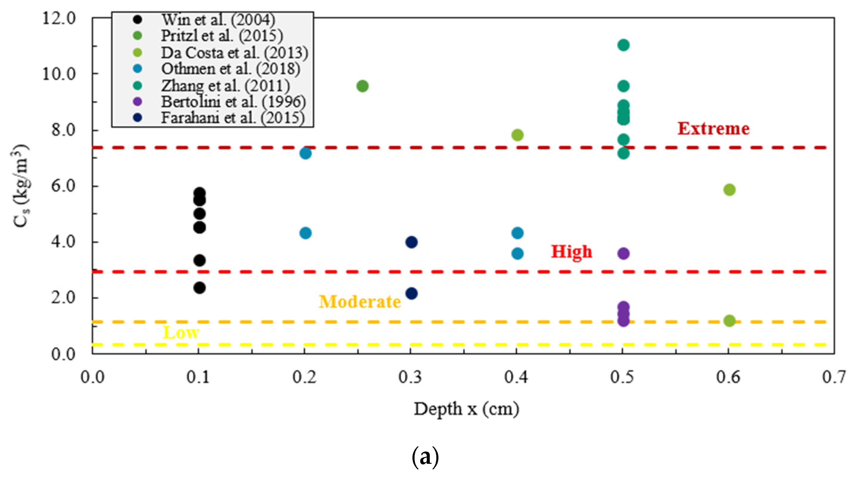
| Moderate | 6 (see Figure 6a) | 1.69 | 0.50 | ||
| High | 15 (see Figure 6a) | 4.96 | 1.21 | ||
| Extreme | 13 (see Figure 6a) | 8.76 | 0.88 | ||
| Cs′ | Low | kg/m3 | – | – | – |
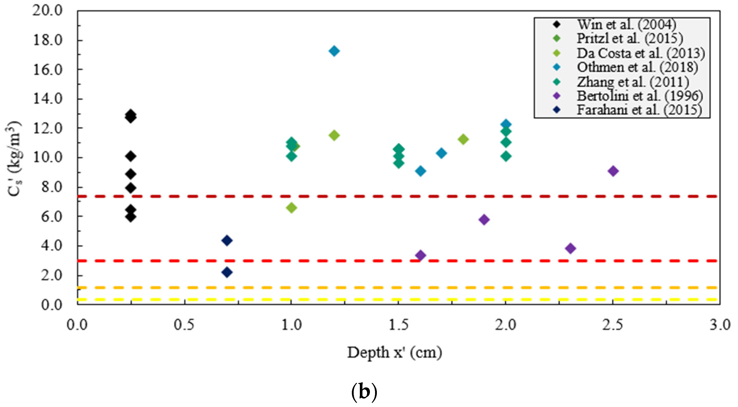
| Moderate | 1 (see Figure 6b) | N/A | N/A | ||
| High | 7 (see Figure 6b) | 5.21 | 1.32 | ||
| Extreme | 26 (see Figure 6b) | 10.91 | 1.78 | ||
| b | Low | kg/m3 | – | – | – |
| Moderate | 6 | 3.84 | 3.53 | ||
| High | 15 | 5.10 | 2.78 | ||
| Extreme | 13 | 1.87 | 0.85 | ||
| Δx | Low | cm | – | – | – |
| Moderate | 6 | 0.91 | 0.63 | ||
| High | 15 | 0.68 | 0.65 | ||
| Extreme | 13 | 1.01 | 0.38 |
| Parameter | Value and reference |
|---|---|
| Inner chloride concentration, C0 | 0.50 kg/m3 [62] |
| Surface chloride concentration, Cs | (see Table 1) |
| Reference factor, f0(w/c) | 4.35 cm2/year [42] a |
| Binding factor, f1(Cb) | 0.85–0.93 (Equation (6)) b |
| Age factor, f3(t) | 0.38–0.75 (Equation (5)) c |
| Deformation/damage factor, f4(ε,d) | 1.73 [38] |
| Modified temperature factor, g1(T,t) | 0.17–1.48 (Equation (16)) d |
| Modified humidity factor, g2(h,t) | 0.13–0.71 (Equation (17)) e |
| Constant diffusivity, D | 0.47 cm2/year (Equation (4)) f |
Publisher’s Note: MDPI stays neutral with regard to jurisdictional claims in published maps and institutional affiliations. |
© 2022 by the authors. Licensee MDPI, Basel, Switzerland. This article is an open access article distributed under the terms and conditions of the Creative Commons Attribution (CC BY) license (https://creativecommons.org/licenses/by/4.0/).
Share and Cite
Zacchei, E.; Bastidas-Arteaga, E. Multifactorial Chloride Ingress Model for Reinforced Concrete Structures Subjected to Unsaturated Conditions. Buildings 2022, 12, 107. https://doi.org/10.3390/buildings12020107
Zacchei E, Bastidas-Arteaga E. Multifactorial Chloride Ingress Model for Reinforced Concrete Structures Subjected to Unsaturated Conditions. Buildings. 2022; 12(2):107. https://doi.org/10.3390/buildings12020107
Chicago/Turabian StyleZacchei, Enrico, and Emilio Bastidas-Arteaga. 2022. "Multifactorial Chloride Ingress Model for Reinforced Concrete Structures Subjected to Unsaturated Conditions" Buildings 12, no. 2: 107. https://doi.org/10.3390/buildings12020107